Island in Charged Black Holes

Abstract

We study the information paradox for the eternal black hole with charges on a doubly-holographic model in general dimensions, where the charged black hole on a Planck brane is coupled to the baths on the conformal boundaries. In the case of weak tension, the brane can be treated as a probe such that its backreaction to the bulk is negligible. We analytically calculate the entanglement entropy of the radiation and obtain the Page curve with the presence of an island on the brane. For the near-extremal black holes, the growth rate is linear in the temperature. Taking both Dvali-Gabadadze-Porrati term and nonzero tension into account, we obtain the numerical solution with backreaction in four-dimensional spacetime and find the quantum extremal surface at $t=0$. To guarantee that a Page curve can be obtained in general cases, we propose two strategies to impose enough degrees of freedom on the brane such that the black hole information paradox can be properly described by the doubly-holographic setup.

¹Institute of High Energy Physics, Chinese Academy of Sciences, Beijing 100049, China
²School of Physics, University of Chinese Academy of Sciences, Beijing 100049, China ³Institute of Theoretical Physics, Chinese Academy of Science, Beijing 100190, China

1 Introduction

The black hole information paradox originates from the problem about whether the information falling into the black hole can eventually sneak out in a unitary fashion. During the evaporation of a black hole, the information carried by the collapsing star appears to conflict with the nearly thermal spectrum of Hawking radiation by semi-classical approximation. One possible explanation comes from quantum information theory. If we assume the chaotic and unitary evaporation of a black hole, then the von Neumann entropy of the radiation may be described by the Page curve, which claims that the entropy will increase until the Page time and then decrease [1, 2, 3], which is in contrast to Hawking’s earlier calculation in which the entropy will keep growing until the black hole totally evaporates [4]. Later, a further debate is raised about whether the ingoing Hawking radiation at late times is burned up at the horizon owing to the “Monogamy of entanglement”, which is known as AMPS firewall paradox [5]. In order to avoid the emergence of firewall, the interior of black hole is suggested to be part of the radiation through an extra geometric connection (see “ER=EPR” conjecture [6]).

Recently AdS/CFT correspondence brings new breakthrough to the understanding of the Page curve from semi-classical gravity and sheds light on how the interior of the black hole projects to the radiation [7, 8, 9]. In this context, the black hole in AdS spacetime is coupled to a flat space, where the latter is considered as a thermal bath.

Motivated by the Ryu-Takayanagi formula and its generalization [10, 11], the fine-grained entropy of a system is calculated by the quantum extremal surface (QES) [12]. When applying this proposal to the evaporation of black holes, an island should appear in the gravity region such that the fine-grained entropy of the radiation is determined by the island formula [13]

$$S_{\mathcal{R}}=\min_{\mathcal{I}}\left\{\mathop{\text{ext}}\limits_{\mathcal{I}}\left[S_{\text{eff}}[\mathcal{R}\cup\mathcal{I}]+\frac{\operatorname{Area}[\partial\mathcal{I}]}{4G_{N}}\right]\right\},$$ (1)

where $\mathcal{R}$ represents the radiation, while the first term is the entanglement entropy of the region $\mathcal{R}\cup\mathcal{I}$, and the second term is the geometrical contribution from the classical gravity. The von Neumann entropy $S_{\mathcal{R}}$ is obtained by the standard process: extremizing over all possible islands $\mathcal{I}$, and then taking the minimum of all extremal values.

A doubly-holographic model has been considered in [13, 14] (see also [15, 16, 17, 18, 19, 20, 21]), in which the matter field in $2D$ black hole geometry is a holographic CFT which enjoys the $AdS_{3}/CFT_{2}$ correspondence. By virtue of this, $S_{\text{eff}}$ in (1) is calculated according to the ordinary HRT formula in $AdS_{3}/CFT_{2}$. At early times, the solution contains no island and the linear increase of the entropy is contributed from the first term in (1) as the accumulation of the Hawking particle pairs. But later, the QES undergoes a phase transition with the emergence of the island $\mathcal{I}$. Meanwhile, owing to the shrinking of the black hole, the decrease of the entropy at late times is dominated by the second term in (1). As a result, the whole process is described by the Page curve and the transition time is the Page time. Moreover, the conjecture of ER=EPR is realized as the fact that the island $\mathcal{I}$ appears in the entanglement wedge of the radiation [6].

A similar information paradox occurs when a two-sided black hole is coupled to two flat baths on each side, and the whole system is in equilibrium [22]. Exchanging Hawking modes entangles black holes and baths. However, according to the subadditivity, the entanglement entropy should be upper bounded at the Page time $t=t_{P}$, namely

$$S_{\mathcal{R}}=S_{\mathcal{B}}\leq S_{\mathcal{B}_{L}}+S_{\mathcal{B}_{R}},$$ (2)

where $\mathcal{B}=\mathcal{B}_{L}\cup\mathcal{B}_{R}$ denotes the two-sided black hole, with $\mathcal{B}_{L}$ and $\mathcal{B}_{R}$ being the black hole on each side, respectively. The equality in (2) comes from the fact that the whole system $\mathcal{R}\cup\mathcal{B}$ is a pure state. The authors in [22] considered the $2D$ eternal black hole-bath system when the whole holographic system is dual to Hartle-Hawking state. Its island extends outside the horizon and the degrees of freedom (d.o.f.) on the island are encoded in the radiation by a geometric connection [22]. A similar conclusion was made independently by only considering the d.o.f. of the radiation [23, 24].

In [25] (see [26] for analytically calculable models, [27, 28, 29] for islands in braneworld and [30, 31] for braneworld holography), a nontrivial setup of the doubly-holographic model for entanglement islands in higher dimensions was established, where the lower dimensional gravity is replaced by a Planck brane with Neumann boundary conditions on it [32, 33, 34]. The solution at $t=0$ was obtained with the DeTurck trick. Moreover, it was demonstrated that the islands exist in higher dimensions, and the main results in [8, 13, 14, 22] can be extended to higher dimensional case as well. However, since the DeTurck trick is inappropriate for the time-dependent case [35, 36], in general, the standard Page curve in higher dimensions is difficult to obtain.

Another issue arises in the context of doubly-holographic setup when one tries to determine the Page time by the initial entropy difference between the solution with island and that without island. If the d.o.f. in the black hole are few compared to the d.o.f. of the baths, then the entropy $S_{\mathcal{R}}$ will saturate at a fairly low level and the inequality (2) has to be saturated at $t=0$ – see Sec. 4.3 for details. That is to say, the Page time is $t_{P}=0$ and thus the Page curve can not be recovered. This phenomenon was firstly noticed in [26] and further elaborated in [37]. To avoid this phenomenon, the essential condition is to input enough d.o.f. into the black hole at the initial time, which is equivalent to increasing the entropy in (1). One immediate resolution is moving the endpoint of the HRT surface away from the brane [25, 26], which is equivalent to transferring d.o.f. from baths into black holes – see Sec. 3.1 for details.

In this paper, we intend to investigate the information paradox in higher dimensional charged black holes. First of all, it is crucial to address the information paradox in four or higher dimensional spacetime. However, to avoid the numerical difficulties, most of early work on the island paradigm were done in 2d or 3d gravity theories. [25] made a significant step to increase the dimensionality by numerical construction and provided an affirmative answer to the question whether the information paradox could be averted by the emergence of an island in higher dimensions, where the AdS-Schwarzschild black hole is considered as the background specifically. In this paper we intend to extend this construction to charged black holes and answer the question whether the island paradigm is a general resolution to the information paradox for higher dimensional black holes. It is reasonable to expect that in this context the island scenario should also be appropriate to describe the entanglement between the black holes and the baths. More importantly, the Page curve is absent in [25] though the relevant discussion and argument support this would be expectable. Therefore in this paper we intend to specifically obtain the Page curve in higher dimensions in the weak tension limit where the backreaction of the brane to the bulk is negligible. We will analytically calculate the entropy of the radiation and evaluate the Page time, which could be viewed as a substantial improvement of the previous work on island in higher dimensions[25]. In addition, taking the charged black hole into account, we are allowed to investigate the Page curve and the Page time at different Hawking temperatures on the unit of the chemical potential, especially in the near extremal case.

The second motivation of our paper is to propose new strategies to avoid the saturation of the entropy at the beginning. Rather than transferring d.o.f. from baths to black holes, we argue that the Planck brane may acquire enough d.o.f. by increasing the tension and adding a Dvali-Gabadadze-Porrati (DGP) term on the brane, which leads to the decrease of the Newton constant $G_{N}$ [30, 31, 27, 28] and thus, increasing the entropy in (1). A more precise description is from the boundary perspective [13], where the $d$-dimensional brane theory is dual to the $(d-1)$-dimensional conformal defect. The d.o.f. on the brane and baths are proportional to central charges in the doubly-holographic model [27]

$$\frac{c_{b}}{c}\sim\left(\frac{l_{\mathrm{eff}}}{L}\right)^{d-2}(1+\lambda_{b}),$$ (3)

where $c_{b}$ is the central charge of the $(d-1)$-dimensional conformal defect, $c$ is the central charge of the $d$-dimensional bath CFT, $L$ is the AdS radius in the bulk, $l_{\mathrm{eff}}$ is the effective AdS radius of the induced metric on the brane and $\lambda_{b}$ is the relative strength of the DGP term. This formula still works near the asymptotic boundary in the presence of black holes. It was shown in [27] that increasing the tension and adding the DGP term (with positive $\lambda_{b}$) enlarges the ratio (3). Furthermore, from numerical calculations, we find that the entropy would not be saturated at the initial time with appropriate tension or DGP term and without transferring any part of the baths into black holes by moving the endpoint of HRT surface away from the brane.

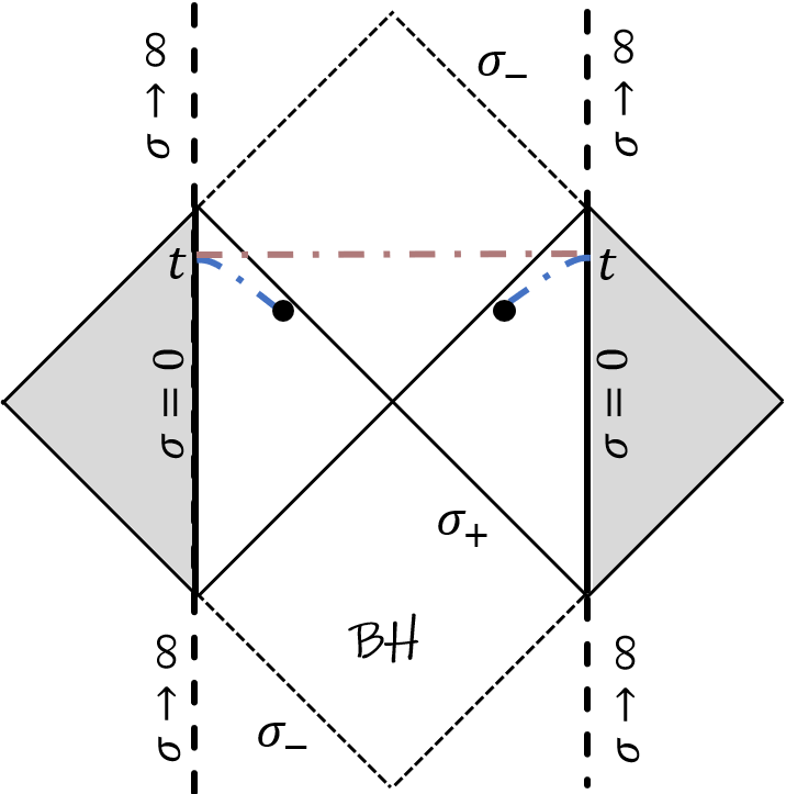
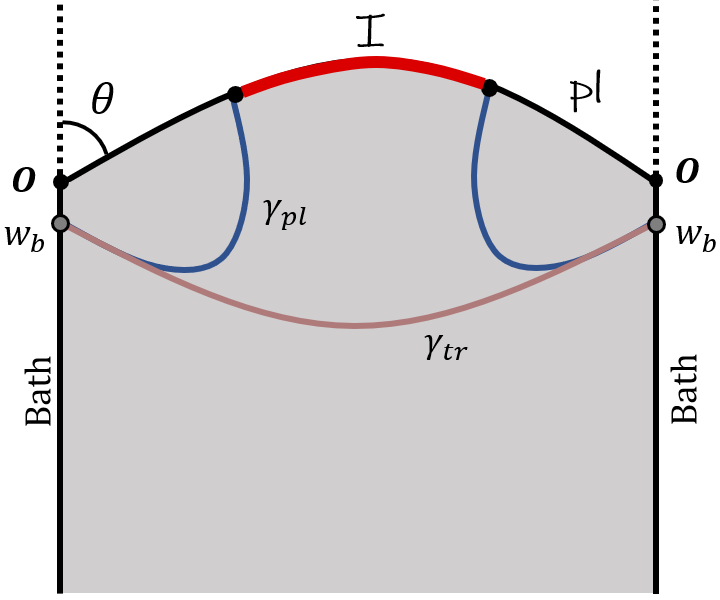
Figure 1: (a): The $d$-dimensional charged black hole is in equilibrium with two flat baths (colored in gray). The conformal boundary is located at $\sigma=0$, while the black hole and baths are distributed in the region with $\sigma>0$ and $\sigma<0$, respectively. Two candidates of the QES at time $t$ are plotted in different colors. (b): A sketch of the $(d+1)$-dimensional dual of the $d$-dimensional holographic system. Here the $d$-dimensional black hole is described equivalently by the Planck brane $\bm{pl}$ in the $(d+1)$-dimensional ambient spacetime. The QES is measured by an ordinary HRT surface (which is plotted as a curve either in blue or rose gold) in the $(d+1)$-dimensional spacetime.

The paper is organized as follows. In section 2, we consider the charged matter on the boundary and build up the doubly-holographic model. In section 3, We neglect the backreaction of the brane and obtain the Page curve in the weak tension limit in general dimensions. The evolution behavior at different Hawking temperature will be demonstrated. In section 4, we take both nonzero tension and DGP term into account, then obtain the numerical solution with backreaction in four-dimensional space time and find the quantum extremal surface at $t=0$. Based on this setup we propose new strategies to avoid the saturation of (2) at $t=0$, and then explore their effects on the island in the back-reacted spacetime. Our conclusions and discussions are given in section 5.

2 The doubly-holographic setup

In this section, we will present the general setup for the island within the charged eternal black hole. We consider a $d$-dimensional charged eternal black hole in $AdS_{d}$ coupled to two flat baths on each side, with the strongly coupled conformal matter living in the bulk, as shown in Fig. 1. On each side, the black hole corresponds to the region with $\sigma>0$ and the bath corresponds to the region with $\sigma<0$. Moreover, at $\sigma=0$, we glue the conformal boundary of the $AdS_{d}$ and flat spacetime together and impose the transparent boundary condition on the matter sector. With a finite chemical potential $\mu$, the matter and the black holes carry charges.

The above description can be equivalently pushed forward into a doubly-holographic setup, where the matter sector is dual to a $(d+1)$-dimensional spacetime and the $d$-dimensional black hole is described by a Planck brane $\bm{pl}$ in the bulk, as shown in Fig. 1. In this paper, we will adopt the doubly-holographic setup.

Consider the action of the $(d+1)$-dimensional bulk as

$$I= \frac{1}{16\pi G_{N}^{(d+1)}}\Bigg{[}\int d^{d+1}x\sqrt{-g}\left(R+\frac{d(d-1)}{L^{2}}\right)+2\int_{\bm{pl}}d^{d}x\sqrt{-h}\left(K-\alpha\right)$$

$$+2\int_{\bm{\partial}}d^{d}x\sqrt{-h_{\bm{\partial}}}K_{\bm{\partial}}-\int d^{d+1}x\sqrt{-g}\frac{1}{2}F^{2}-2\int_{\bm{pl}\cap\bm{\partial}}d^{d-1}x\sqrt{-\Sigma}\,\theta\Bigg{]}.$$ (4)

Here $K$ is the extrinsic curvature and the parameter $\alpha$ is proportional to the tension on the brane $\bm{pl}$, which will be fixed later. $K_{\bm{\partial}}$ is the extrinsic curvature on the conformal boundary $\bm{\partial}$. The electromagnetic curvature is $F=\text{d}A$. The last term is the junction term at the intersection of the brane $\bm{pl}$ and the conformal boundary $\bm{\partial}$, where $\theta$ is the angle between the brane and the boundary, while $\Sigma$ is the metric on $\bm{pl}\cap\bm{\partial}$. Taking the variation of the action, we obtain the equations of motion as

$$R_{\mu\nu}+\frac{d}{L^{2}}g_{\mu\nu} =\left(T_{\mu\nu}-\frac{T}{d-1}g_{\mu\nu}\right),\quad\text{with}\quad T_{\mu\nu}=F_{\mu a}F_{\nu}{}^{a}-\frac{1}{4}F^{2}g_{\mu\nu},$$ (5)

$$\nabla_{\mu}F^{\mu\nu} =0,$$ (6)

where $T$ is the trace of the energy-stress tensor $T_{\mu\nu}$.

2.1 The Planck brane

In AdS/CFT setup with infinite volume, the $(d+1)$-dimensional bulk is asymptotic to $AdS_{d+1}$ which in Poincaré coordinates is described by

$$ds^{2}=\frac{L^{2}}{z^{2}}\left(-dt^{2}+dz^{2}+dw^{2}+\sum_{i=1}^{d-2}dw_{i}^{2}\right),$$ (7)

with the conformal boundary at $z=0$. Let $\theta$ be the angle between the Planck brane and the conformal boundary as shown in Fig. 2. Then the Planck brane $\bm{pl}$ is described by the hypersurface

$$z+w\tan\theta=0,$$ (8)

near the boundary. One should cut the bulk on the brane $\bm{pl}$ and restrict it in the region with $z+w\tan\theta>0$ [38, 39, 40, 32]. We will also impose this constraint (8) deep into the bulk and find its back-reaction to the geometry.

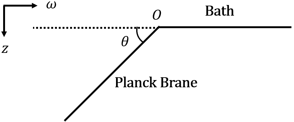
Figure 2: A simple setup of Randall-Sundrum brane[32]. Here the Planck brane is anchored on the conformal boundary at $(z,w)=(0,0)$ and penetrates into the bulk with an angle $\theta$.

As for the boundary term in (2), we impose a Neumann boundary condition on the Planck brane which is

$$K_{ij}-Kh_{ij}+\alpha h_{ij}=0,$$ (9)

where $h_{ij}$ is the induced metric on the brane $\bm{pl}$ . The parameter $\alpha$ in action (2) is fixed to be a constant by solving (9) near the conformal boundary to concrete the tension term on the brane.

In addition to (9), we also impose the Neumann boundary condition for gauge field $A_{\mu}$ on the brane $\bm{pl}$ [32, 41, 33, 34], which is

$$n^{\mu}F_{\mu\nu}h^{\nu}{}_{i}=0,$$ (10)

where $n_{\mu}$ is the normal vector to the brane and $i$ denotes the coordinates along the brane.

2.2 The quantum extremal surface

The von Neumann entropy of the radiation $\mathcal{R}$ in (1) is measured by the QES . There are two sorts of candidate for the QES. One sort of candidate is the disconnected surface, which is represented by the partial Cauchy surfaces in blue ended with the black dot, while the other is the connected surface, which is represented by the partial Cauchy surface in rose gold, as illustrated in Fig. 1. Mapping into the doubly-holographic description, the QES is equivalently described by a $(d-1)$-dimensional HRT surface [25], namely

$$S_{\mathcal{R}}=\min_{\mathcal{I}}\left[\frac{\text{Area}(\gamma_{\mathcal{I}\cup\mathcal{R}})}{4G_{N}^{(d+1)}}\right],$$ (11)

where $\gamma_{\mathcal{I}\cup\mathcal{R}}$ is the HRT surface sharing the boundary with $\mathcal{I}\cup\mathcal{R}$, as illustrated in Fig. 1. In this figure, each candidate of the HRT surface corresponds to a co-dimension two surface $\gamma_{\mathcal{I}\cup\mathcal{R}}$ in the bulk. One is a trivial surface $\gamma_{tr}$ anchored on the left and right baths, and the island $\mathcal{I}$ is absent; the other is a surface $\gamma_{pl}$ anchored on the Planck brane $\bm{pl}$ with non-trivial island $\mathcal{I}$ on the brane. The emergence of island $\mathcal{I}$ keeps the von Neumann entropy (1) from divergence after the Page time [22].

Consider a HRT surface anchor at $w=w_{b}$ on the boundary – Fig. 1. It measures the entanglement between two subsystems. One consists of the brane $\bm{pl}$ and part of baths within the region $0<w\leq w_{b}$. Conventionally we still call this subsystem as black hole subsystem hereafter. While the other subsystem consists of the remaining bath with $w>w_{b}$, and we simply call it as the radiation subsystem.

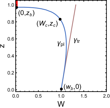
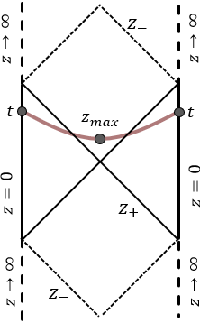
Figure 3: (a): For $\{d,T_{h}/\mu,\theta,w_{b}/\mu\}=\{3,0.45757,2\pi/5,2\}$, two candidates $\gamma_{tr}$ and $\gamma_{pl}$ are colored in rose gold and blue, respectively. Half of the island is colored in red. (b): The trivial surface $\gamma_{tr}$ is colored in rose gold at time $t$, where $z_{max}$ is the turning point with $z^{\prime}|_{z_{max}}=0$.

3 Entropy density without back-reaction

Page curve plays a vital role in understanding the information paradox. In this section, we will firstly compute the entropy density by figuring out the quantum extremal surface in the weak tension limit. In such a case, the Planck brane $\bm{pl}$ can be treated as a probe and its back-reaction to the background geometry is ignored. Next we consider the growth of the entropy density with the time. By properly choosing the endpoint of HRT surface, we plot the Page curve at different Hawking temperature and evaluate the Page time.

3.1 The entropy density in the RN black hole

Define

$$W=z\cot\theta+w$$ (12)

such that the Planck brane $\bm{pl}$ is located at $W=0$ and we only take part of the manifold with $W\geq 0$ into account. The tension on the brane is

$$\alpha=(d-1)\cos\theta/L.$$ (13)

When the tension is weak ($\theta\rightarrow\pi/2$), the brane $\bm{pl}$ applies no back-reaction to the background, and the geometry can be regarded as the planar RN-AdS_d+1, which is

$$ds^{2} =\frac{L^{2}}{z^{2}}\left[-f(z)dt^{2}+\frac{dz^{2}}{f(z)}+(dW-\cot\theta dz)^{2}+\sum_{i=1}^{d-2}dw_{i}^{2}\right],$$ (14)

$$A= \mu\left(1-z^{d-2}\right)dt,$$ (15)

$$f(z)= 1-\left(1+\frac{d-2}{d-1}\mu^{2}\right)z^{d}+\frac{d-2}{d-1}\mu^{2}z^{2d-2},$$ (16)

where $\mu$ is the chemical potential of the system on the boundary. The horizon has been rescaled to $z=1$ and one can recover it by transforming coordinates

$$\{t,z,W,w_{i}\}\to\{t,z,W,w_{i}\}z_{h}^{-1},\quad i=1,2,...,d-2$$ (17)

In coordinates (14), the Hawking temperature is fixed to be

$$T_{h}=\frac{d(d-1)-(d-2)^{2}\mu^{2}}{4\pi(d-1)}$$ (18)

From (11), the entropy density of the radiation subsystem is determined by the minimum

$$\tilde{S}_{\mathcal{R}}=\frac{S_{\mathcal{R}}}{V_{d-2}}=2\min\left(\mathop{\text{ext}}\limits_{z_{b}}\left[\tilde{S}_{pl}(z_{b})\right],\tilde{S}_{tr}\right).$$ (19)

Here $V_{d-2}=\prod_{i}^{d-2}\int dw_{i}$ is the volume of the relevant spatial directions and $z_{b}$ is the intersection of $\gamma_{pl}$ and the brane. For simplicity, all the above thermodynamic quantities are dimensionless. Following the transformation (17), their dimensions can be recovered as

$$\left\{T_{h},\mu,V_{d-2},S,\tilde{S}\right\}\to\left\{T_{h}\,z_{h},\mu\,z_{h},V_{d-2}z_{h}^{2-d},S,\tilde{S}\,z_{h}^{d-2}\right\},$$ (20)

where $S$ and $\tilde{S}$ refer to any entropy and its density. Throughout this paper, all the dimensional quantities will be illustrated on the unit of chemical potential $\mu$.

Noticed that $\gamma_{pl}$ becomes a candidate of the QES only after taking the extremum. $\mathop{\text{ext}}\limits_{z_{b}}\left[\tilde{S}_{pl}(z_{b})\right]$ and $\tilde{S}_{tr}$ are the entropy density contributed by the two candidates respectively – see Fig. 3. The entropy density of the radiation subsystem is identified as the minimum of these quantities.

Firstly, we consider the surface $\gamma_{pl}$ ended on the Planck brane at $z_{b}$. Two different parameterizations may be introduced on different intervals, just as performed in [25]. In $(W,z)$ plane as illustrated in Fig. 3, we introduce $W=W(z)$ for the curve segment in $z\in[0,z_{c}]$, while for the segment in $W\in[0,W_{c}]$, we introduce $z=z(W)$ instead, with $z^{\prime}(W_{c})=W^{\prime}(z_{c})^{-1}$. As a result, the density functional can be evaluated by the area of the surface $\gamma_{pl}$ intersecting the brane at $z_{b}=z(0)$, and the corresponding expression is

$$\tilde{S}_{pl}(z_{b})= \frac{L^{d-1}}{4G_{N}^{(d+1)}}\Bigg{(}\int_{0}^{z_{c}}\frac{dz}{z^{d-1}}\sqrt{\frac{f(z)\left[\cot\theta-W^{\prime}(z)\right]^{2}+1}{f(z)}}$$

$$+\int_{0}^{W_{c}}\frac{dW}{z(W)^{d-1}}\sqrt{\frac{f[z(W)]\left[\cot\theta z^{\prime}(W)-1\right]^{2}+z^{\prime}(W)^{2}}{f[z(W)]}}\Bigg{)}.$$ (21)

Since $z_{b}$ depends on $(W_{c},z_{c})$, $\tilde{S}_{pl}(z_{b})$ can be view as a function of $z_{b}$. In Fig. 3, $W=w_{b}$ is the location where $\gamma_{pl}$ is anchored on the conformal boundary $z=0$.

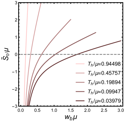
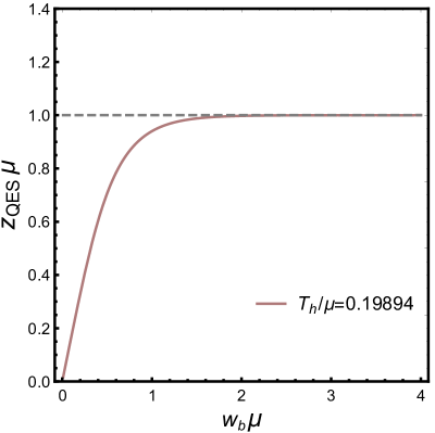
Figure 4: (a): For $d=3$ and $\theta=\pi/2$, the relations between the density difference and the end point of the HRT surface are plotted at different temperatures. (b): The location of QES $z_{{}_{QES}}$ as a function of $w_{b}\mu$, with $\{d,\theta\}=\{3,\pi/2\}$.

Next we consider the entropy density associated with the surface $\gamma_{tr}$ penetrating the horizon as the QES. Since $\gamma_{tr}$ keeps growing due to the growth of the black hole interior in the $(d+1)$-dimensional ambient geometry [42], we express the area functional in the Eddington-Finkelstein coordinates and the entropy density $\tilde{S}_{tr}(t)$ becomes

$$\tilde{S}_{tr}(t)=\frac{L^{d-1}}{4G_{N}^{(d+1)}}\int\frac{d\xi}{z(\xi)^{d-1}}\sqrt{-v^{\prime}(\xi)\left[f(z(\xi))v^{\prime}(\xi)+2z^{\prime}(\xi)\right]},$$ (22)

where $\xi$ is the intrinsic parameter on $\gamma_{tr}$ (Fig. 3) and

$$t=v+\int\frac{dz}{f(z)}.$$

Given the surface $\gamma_{tr}$ which penetrates the horizon at $t=0$ and the surface $\gamma_{pl}$ which is anchored on the boundary at any $z_{b}$, we define their density difference as

$$\tilde{S}_{0}[z_{b}]=2\left(\tilde{S}_{pl}(z_{b})-\tilde{S}_{tr}(0)\right).$$ (23)

Then the corresponding entropy density difference between two QES candidates is given by

$$\tilde{S}_{0}=\mathop{\text{ext}}\limits_{z_{b}}\tilde{S}_{0}[z_{b}]=2[\tilde{S}_{pl}(z_{{}_{QES}})-\tilde{S}_{tr}(0)],$$ (24)

where $\tilde{S}_{0}[z_{b}]$ exhibits its extremum at $z_{b}=z_{{}_{QES}}$. Then the entropy density of the radiation subsystem $\tilde{S}_{\mathcal{R}}$ at the initial time depends on the sign of $\tilde{S}_{0}$ as follows: If $\tilde{S}_{0}>0$, then $\gamma_{tr}$ is the HRT surface at $t=0$, which provides a good starting point for the evolution of the entanglement between the black hole subsystem and the radiation subsystem. In this case $\tilde{S}_{tr}(t)$ keeps growing with time $t$ and at some moment it must reach the entropy density of $\tilde{S}_{pl}(z_{{}_{QES}})$ . After that, the HRT surface becomes $\gamma_{pl}$ such that $\tilde{S}_{\mathcal{R}}$ stops growing at the Page time $t_{P}$. On the contrary, if $\tilde{S}_{0}<0$, then the inequality (2) has to be saturated at the beginning, indicating that $\gamma_{pl}$ has already been the HRT surface at $t=0$ and no Page curve appears.

In next subsection, we intend to discuss the negativity of $\tilde{S}_{0}$ in detail and point out that the negative $\tilde{S}_{0}$ results from the lack of d.o.f. in the black hole subsystem. We will demonstrate that to avoid the negativity of $\tilde{S}_{0}$, one may input enough d.o.f. into the black hole subsystem by choosing relatively large $w_{b}$, as carried out in [26].

3.2 On the difference of the entropy density

First of all, we plot the relation between $\tilde{S}_{0}$ and the location of the endpoint $w_{b}$ of the HRT surface in Fig. 4. It is noticed that generically $\tilde{S}_{0}$ exhibits a monotonous behavior with $w_{b}$. Specifically it is negative for small endpoint $w_{b}$, which leads to the saturation of the inequality (2) at $t_{P}=0$. Previously similar phenomenon was observed in [26] with zero tension on the brane. On the other hand, for large $w_{b}$ the difference of the entropy density is always positive and thus appropriate for the Page evolution. Next we intend to argue that different choices of $w_{b}$, in effect, lead to different divisions of the whole system into the black hole subsystem and the radiation subsystem. Specifically, the solution with $w_{b}=0$ measures the entanglement between the brane and their complementary, namely the whole baths. While for positive $w_{b}$, part of baths within $W\leq w_{b}$ is counted into the black hole subsystem, and the QES measures the entanglement between a new black hole subsystem which contains some d.o.f. of baths and the radiation subsystem at $W>w_{b}$.

Moreover, the amount of the d.o.f. on the brane encoded in the radiation subsystem depends on the endpoint $w_{b}$. To make this point transparent, we plot the location of QES $z_{{}_{QES}}:=z(0)$ as a function of $w_{b}\mu$ in Fig. 4. We find that the island is always stretching out of the horizon ($z_{{}_{QES}}\mu<1$), indicating that besides the interior, the region near the exterior of the horizon will also be encoded in the radiation subsystem by the entanglement wedge. This result is consistent with that in [22] and reflects the spirit of the ER$=$EPR proposal, which suggests that two distant systems are connected by some geometric structure. For $w_{b}\mu\rightarrow 0$, the location of QES also approaches $z_{{}_{QES}}\mu\rightarrow 0$, which indicates that the whole region outside the horizon is likely to be encoded in the radiation subsystem. While for large $w_{b}\mu$, $z_{{}_{QES}}\mu$ approaches the horizon, which implies that more d.o.f. in baths are counted into the black hole subsystem, the less region on the brane is encoded in the radiation subsystem.

In the remainder of this section, we will choose sufficiently large $w_{b}$ to guarantee that $\tilde{S}_{0}$ is positive and then explore the evolution of the von Neumann entropy of the radiation subsystem. In Sec. 4, once the backreaction is taken into account, we will present new strategies to avert the negativity of $\tilde{S}_{0}$, by inputting more d.o.f. on the brane directly, rather than transferring some d.o.f. from baths.

3.3 Time evolution of the entropy density

We are interested in the growth of the entropy density with the time, thus we define

$$\Delta\tilde{S}(t)=\tilde{S}_{\mathcal{R}}(t)-2\tilde{S}_{tr}(0)=\begin{cases}2\tilde{S}_{tr}(t)-2\tilde{S}_{tr}(0),&{t<t_{P}}\\ \tilde{S}_{0},&{t\geq t_{P}}\end{cases}$$ (25)

which is free from the UV divergence and its saturation equals the density difference $\tilde{S}_{0}$ as we defined in Sec. 3.1. For large endpoints $w_{b}$, we have $\tilde{S}_{0}>0$ and the growth rate of $\Delta\tilde{S}(t)$ is obtained similarly with the method applied in [43]. Since the integrand of (22) does not depend explicitly on $v$, one can derive a conserved quantity as

$$C=\frac{f(z)v^{\prime}+z^{\prime}}{z^{d-1}\sqrt{-v^{\prime}\left[f(z)v^{\prime}+2z^{\prime}\right]}}.$$ (26)

It is also noticed that the integral shown in (22) is invariant under the reparametrization, hence the integrand can be chosen freely as

$$\sqrt{-v^{\prime}\left[f(z)v^{\prime}+2z^{\prime}\right]}=z^{d-1}.$$ (27)

Substituting (26) and (27) into (22), we have

$$\frac{d}{dt}\tilde{S}_{tr} =\frac{L^{d-1}}{4G_{N}^{(d+1)}}\frac{\sqrt{-f(z_{max})}}{z_{max}^{d-1}},$$ (28)

$$t =\int_{0}^{z_{max}}dz\frac{Cz^{d-1}}{f(z)\sqrt{f(z)+C^{2}z^{2d-2}}}.$$ (29)

Here $z_{max}$ is the turning point of trivial surface $\gamma_{tr}$ as shown in Fig. 3, and the relation between $z_{max}$ and the conserved quantity $C$ is given by

$$f(z_{max})+C^{2}z_{max}^{2d-2}=0.$$ (30)

At later time, the trivial extremal surface $\gamma_{tr}$ tends to surround a special extremal slice $z=z_{M}$, as shown in [42]. Define

$$F(z):=\frac{\sqrt{-f(z)}}{z^{d-1}},$$ (31)

we find that $C^{2}=F(z_{max})^{2}$ keeps growing until meeting the extremum at $z_{max}=z_{M}$, where we have

$$F^{\prime}(z_{M})=(1-d)z_{M}^{-d}\sqrt{-f\left(z_{M}\right)}-\frac{z_{M}^{1-d}f^{\prime}\left(z_{M}\right)}{2\sqrt{-f\left(z_{M}\right)}}=0.$$ (32)

By solving (32), we finally obtain the evolution of the entropy density as

$$\lim_{t\rightarrow\infty}\frac{d}{dt}\tilde{S}_{tr}=\frac{L^{d-1}}{4G_{N}^{(d+1)}}\;F(z_{M}).$$ (33)

Next we discuss the growth rate of entropy density for the neutral case and the charged case separately. Since the saturation occurs at $\tilde{S}_{0}$, the Page time is approximately expressed as

$$t_{P}\approx\frac{\tilde{S}_{0}}{d\tilde{S}_{tr}/dt}.$$ (34)

• The Neutral Case: For $\mu=0$, substituting $f(z)=1-z^{d}$ into (32), after recovering the dimension (17)(20), we have the growth rate of entropy density at late times as

  $$\lim_{t\rightarrow\infty}\frac{d}{dt}\tilde{S}_{tr}=c_{d}\frac{L^{d-1}}{4G_{N}^{(d+1)}}T_{h}^{d-1}$$ (35)

  where $c_{d}=2^{2d+\frac{1}{d}-3}\pi^{d-1}d^{\frac{3}{2}-d}(-1+d)^{\frac{1-d}{d}}(-2+d)^{\frac{d-2}{2d}}$. For $d=2$, $c_{d}=2\pi$ and the growth rate is proportional to Hawking temperature of the black hole, which is exactly in agreement with the result in [22, 42].

  Due to the exchanging of Hawking modes, the entanglement entropy of the radiation subsystem grows linearly during most of time at a rate proportional to $T_{h}^{d-1}$. If there was no island, the entanglement entropy would keep growing and finally exceeding the maximal entropy the black hole subsystem allowed to contain. It would be an information paradox similar to the version of evaporating black hole. The formation of quantum extremal surface with island at Page time resolves this paradox, since some d.o.f. on the brane are encoded in the radiation subsystem and the entanglement entropy stops growing and becomes saturated.

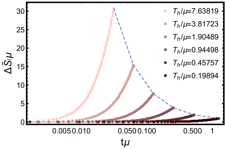
Figure 5: For $\{d,w_{b},L,\theta\}=\{3,1,1,9\pi/20\}$, the Page curves are plotted for different Hawking temperatures. The dashed curve in blue connects the Page time $t=t_{P}$ of each Page curve. In the plot, The Newton constant is fixed to be $\frac{L^{2}}{4G_{N}^{(4)}}=1$.

• The Charged Case: Recall that in general dimensions, when turning on the chemical potential, the blackening factor becomes

  $$f(z)=1-\left(1+\frac{d-2}{d-1}\mu^{2}\right)z^{d}+\frac{d-2}{d-1}\mu^{2}z^{2d-2}.$$ (36)

  The growth rate of entanglement entropy with $d\geq 3$ at late times is obtained by substituting the above equation into (32), which is

  $$\lim_{t\rightarrow\infty}\frac{d}{dt}\tilde{S}_{tr}= \frac{L^{d-1}}{4G_{N}^{(d+1)}}\left(\frac{2(d-1)^{2}}{(d-2)(d-1+(d-2)\mu^{2})}\right)^{\frac{1-d}{d}}$$

  $$\sqrt{-1+\frac{2(d-1)}{d-2}-\frac{d-2}{d-1}\left(\frac{2(d-1)^{2}}{(d-2)(d-1+(d-2)\mu^{2})}\right)^{\frac{2(d-1)}{d}}\mu^{2}}.$$ (37)

  Specially, after recovering the dimension (17)(20), the growth rate for the near-extremal black hole is

  $$\lim_{t\rightarrow\infty\atop T_{h}\to 0}\frac{d}{dt}\tilde{S}_{tr}=\frac{L^{d-1}}{4G_{N}^{(d+1)}}2\pi\sqrt{\frac{1}{d(d-1)}}\left[\frac{d(d-1)}{(d-2)^{2}}\right]^{\frac{2-d}{2}}T_{h}\mu^{d-2}.$$ (38)

  The linear-$T_{h}$ behavior comes from the AdS${}_{2}\times R^{d-1}$ space, which is the near horizon geometry of the near-extremal black hole.

  Some numerical results are shown in Fig. 5. When $T_{h}/\mu\gg 1$, the entropy density approach the neutral case as mentioned above, which has a high growth rate and a large saturated value. When $T_{h}/\mu\ll 1$, the entropy density has a low growth rate and a small saturated value. At the extremal case $T/\mu\to 0$, the evolution is nearly frozen and the entanglement entropy barely grows.

Since the entanglement between the black hole and the radiation subsystem is built up by the exchanging of Hawking modes before the Page time $t_{P}$, the phenomenon that entropy increases rapidly at higher temperatures indicates that the higher the Hawking temperature is, the higher the rate of exchanging is.

4 Entropy with back-reaction

In this section we will consider the QES in the presence of the island when the back-reaction of the Plank brane to the bulk is taken into account for $d=3$. First of all, we will introduce a DGP term on the brane, and discuss its effects on the setup. Next, we will provide new strategies to enhance the d.o.f on the brane such that the entropy density difference is guaranteed to be positive at the initial time. After that, we will apply the DeTurck trick to handle the static equations of motion and find the numerical solution to the background with backreaction at $t=0$ via spectrum method. Finally, the effects of the tension and the DGP term on the evolution will be investigated.

4.1 The DGP term

We introduce the action of a $d$-dimensional brane into (2) as

$$I_{b}=\frac{1}{16\pi G_{b}^{(d)}}\int d^{d}x\sqrt{-h}R_{h}+\frac{1}{8\pi G_{b}^{(d)}}\int_{\bm{pl}\cap\bm{\partial}}d^{d-1}x\sqrt{-\Sigma}\,k.$$ (39)

The first term on the r.h.s is the DGP term [27], where $G_{b}^{(d)}$ is the additional Newton constant on the brane and $R_{h}$ is the intrinsic curvature on the brane. The second term is the junction term at the intersection $\bm{pl}\cap\bm{\partial}$ of the brane and the conformal boundary, where $\Sigma$ is the metric on $\bm{pl}\cap\bm{\partial}$ and $k$ is the extrinsic curvature on $\bm{pl}\cap\bm{\partial}$.

For the boundary term in (2) and (39), the new Neumann boundary conditions are

$$K_{ij}-Kh_{ij}+\alpha h_{ij}=\lambda L\left[\frac{1}{2}R_{h}h_{ij}-(R_{h}){}_{ij}\right],$$ (40)

where $\lambda\equiv\frac{G_{N}^{(d+1)}}{G_{b}^{(d)}L}$ can be regarded as the effective coupling of the DGP term. The parameter $\alpha$ in action (2) is now obtained by solving (40) near the conformal boundary to concrete the tension term on the brane.

The von Neumann entropy of the radiation subsystem $\mathcal{R}$ in (1) is now equivalently described by a $(d-1)$-dimensional HRT surface and a lower-dimensional area term on the brane $\bm{pl}$ [27, 28, 29], namely

$$S_{\mathcal{R}}=\frac{1}{4G_{N}^{(d+1)}}\,\min_{\mathcal{I}}\left[\mathop{\text{ext}}\limits_{\mathcal{I}}[\textbf{Area}(\gamma_{\mathcal{I}\cup\mathcal{R}})+\lambda L\,\textbf{Area}(\partial\mathcal{I})]\right],$$ (41)

where $\gamma_{\mathcal{I}\cup\mathcal{R}}$ is the HRT surface sharing the boundary with $\mathcal{I}\cup\mathcal{R}$.

4.2 The metric ansatz

We introduce the Deturck method [36] to numerically solve the background in the presence of the Planck brane in this subsection, and the numerical results for the QES over such backgrounds will be presented in next subsection. Instead of solving (5) directly, we solve the so-called Einstein-DeTurck equation, which is

$$R_{\mu\nu}+3\,g_{\mu\nu} =\left(T_{\mu\nu}-\frac{T}{2}g_{\mu\nu}\right)+\nabla_{(\mu}\xi_{\nu)},$$ (42)

where

$$\xi^{\mu}:=\left[\Gamma_{\nu\sigma}^{\mu}(g)-\Gamma_{\nu\sigma}^{\mu}(\bar{g})\right]g^{\nu\sigma}$$

is the DeTurck vector and $\bar{g}$ is the reference metric, which is required to satisfy the same boundary conditions as $g$ only on Dirichlet boundaries, but not on Neumann boundaries [25].

	1	2	3	4	5	6
$\mathbf{y=1}$	$Q_{1}=1$	$Q_{2}=1$	$Q_{3}=\cot\theta$	$Q_{4}=1$	$Q_{5}=1$	$\psi=\mu$
$\mathbf{y=0}$	$\partial_{y}Q_{1}=0$	$\partial_{y}Q_{2}=0$	$\partial_{y}Q_{3}=0$	$\partial_{y}Q_{4}=0$	$\partial_{y}Q_{5}=0$	$\partial_{y}\psi=0$
$\mathbf{x=1}$	$Q_{1}=1$	$Q_{2}=1$	$Q_{3}=\cot\theta$	$Q_{4}=1$	$Q_{5}=1$	$\psi=\mu$
$\mathbf{x=0}$	$n^{\mu}F_{\mu\nu}h^{\nu}{}_{i}=0$	$n_{\mu}\xi^{\mu}=0$	$Q_{3}=\cot\theta$	Equation (40)

Table 1: Boundary conditions.

Now we introduce the metric ansatz and the boundary conditions in the doubly-holographic setup. For $W\rightarrow\infty$, the ambient geometry is asymptotic to $4D$ planar RN-AdS black (14) with $d=3$. Furthermore, for numerical convenience we define two new coordinates in the same way as applied in [25], which are

$$x=\frac{W}{1+W}\qquad\text{and}\qquad y=\sqrt{1-z}.$$ (43)

The domain of the first coordinate $x$ is compact, while the second coordinate $y$ keeps the metric from divergence at the outer horizon $y_{+}=0$.

When the back-reaction of the Planck brane is taken into account, the translational symmetry along $x$ direction is broken. Therefore, the most general ansatz of the background is

$$ds^{2}= \frac{L^{2}}{(1-y^{2})^{2}}\left[-y^{2}P(y)Q_{1}dt^{2}+\frac{4Q_{2}}{P(y)}dy^{2}+\frac{Q_{4}}{(1-x)^{4}}\left(dx+2y(1-x)^{2}Q_{3}dy\right)^{2}+Q_{5}dw_{1}^{2}\right]$$ (44)

$$A= y^{2}\,\psi\,dt,$$ (45)

$$P(y)= 2-y^{2}+(1-y^{2})^{2}-\frac{1}{2}(1-y^{2})^{3}\mu^{2}.$$ (46)

where $\left\{Q_{1},Q_{2},Q_{3},Q_{4},Q_{5},\psi\right\}$ are the functions of $\left(x,y\right)$. All the boundary conditions are listed in Tab. 1 , with

$$\alpha=\left(2\cos\theta-\lambda\sin^{2}\theta\right)/L.$$ (47)

Moreover, the boundary conditions at the horizon $y=0$ also imply that $Q_{1}(x,0)=Q_{2}(x,0)$, which fixes the temperature of the black hole (18) as

$$T_{h}=\frac{6-\mu^{2}}{8\pi}.$$ (48)

The reference metric $\bar{g}$ is given by $Q_{1}=Q_{2}=Q_{4}=Q_{5}=1$ and $Q_{3}=\cot\theta$. In this case, the corresponding charge density $\rho$ decays from the Planck brane $\bm{pl}$ to the region deep into the bath as shown in Fig. 6.

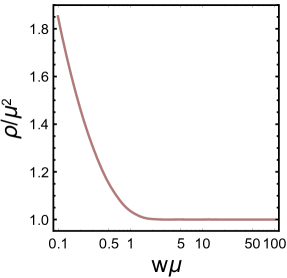
Figure 6: The charge density in the case for $\{T_{h}/\mu,\theta,\lambda\}=\{0.19894,\pi/4,1\}$.

4.3 New prescriptions for the saturation at $t=0$

Firstly, let us elaborate the whole evaporation process in a specific manner. At the beginning of the evolution, two black holes $\mathcal{B}_{L}$ and $\mathcal{B}_{R}$ are entangled with each other. As time passes by, the black holes interact with environment (radiation) by exchanging the hawking modes, and the von Neumann entropy of the radiation increases. At the Page time, two black holes are disentangled with each other and fully entangled with the environment. At the same time, the von Neumann entropy of the radiation saturates.

If black holes $\mathcal{B}_{L}$ and $\mathcal{B}_{R}$ lack of d.o.f., they might be disentangled at the beginning of the evolution. Therefore, the conditions leading to the negative density difference $\tilde{S}_{0}$ cannot capture the dynamics of the intermediate stage, and is not appropriate to the information paradox for black holes – see also Sec. 3.

Based on above observation, we argue that to obtain a Page curve successfully in the context of eternal black holes, the essential condition is to input sufficient d.o.f. into the black hole subsystem, that will increase the entropy in (1). In the weak tension limit as discussed in previous section, we implement this by choosing the endpoint of HRT surface with large $w_{b}$, which actually just transfer some d.o.f. from baths to the black hole subsystem. Now once the backreaction is taken into account, we have more strategies to enhance the d.o.f. on the brane directly, which from our point of view should be more natural to address the information paradox for the eternal black hole. To realize it, the key point is to decrease the $d$-dimensional Newton constant [30, 31, 27, 28]. Therefore, one possible way is to increase the tension on the brane by adjusting the value of $\theta$ from $\pi/2$ to $0$ – see (13) and (47). Alternatively, one may increase the effects of the intrinsic curvature term (DGP term) on the brane by adjusting the DGP coupling $\lambda$ – see (52).

In the remainder of this section, we will demonstrate that above strategies works well in giving rise to a positive $\tilde{S}_{0}$, even with $w_{b}=0$.

4.4 The entropy density in the back-reacted spacetime

In this subsection, all free parameters will be fixed for numerical analysis. To regularize the UV divergence of entropy, we should introduce a UV cut-off. Since $\gamma_{pl}$ and $\gamma_{tr}$ share the same asymptotic behavior, their difference should be independent of the cut-off given that it is small enough. We find that the UV cut-off $y_{\epsilon}=1-1/100$ is good enough for numerical calculation.

From (41), the entropy density of the radiation subsystem $\tilde{S}_{\mathcal{R}}$ is now determined by

$$\tilde{S}_{\mathcal{R}}=2\min\left(\mathop{\text{ext}}\limits_{y_{b}}\left[\tilde{S}_{pl}(y_{b})+\tilde{S}_{{}_{DGP}}(y_{b})\right],\tilde{S}_{tr}\right).$$ (49)

Here $y_{b}$ is the intersection of $\gamma_{pl}$ with the brane. Notice that $\gamma_{pl}$ is not a candidate of the QES until taking the extremum. $\mathop{\text{ext}}\limits_{y_{b}}\left[\tilde{S}_{pl}(y_{b})+\tilde{S}_{{}_{DGP}}(y_{b})\right]$ and $\tilde{S}_{tr}$ are the entropy density of two candidates respectively, while the entropy density of the radiation subsystem is identified with the minimum of two candidates. Next, we derive the expressions for the entropy density of two candidates in a parallel way as presented in the previous section.

For the trivial surface $\gamma_{tr}$ at $t=0$ as the QES, we introduce the parameterization $x=x(y)$, which leads to the corresponding entropy density

$$\tilde{S}_{tr}(0)=\frac{L^{2}}{4G_{N}^{(4)}}\int_{0}^{1}dy\frac{1}{\left(1-y^{2}\right)^{2}}\sqrt{Q_{5}\left(\frac{4Q_{2}}{P(y)}+\frac{Q_{4}\left(2y(x(y)-1)^{2}Q_{3}+x^{\prime}(y)\right)^{2}}{(x(y)-1)^{4}}\right)}.$$ (50)

For numerical convenience, we have set ${L^{2}/(4G_{N}^{(4)})}=1$ in the following discussion.

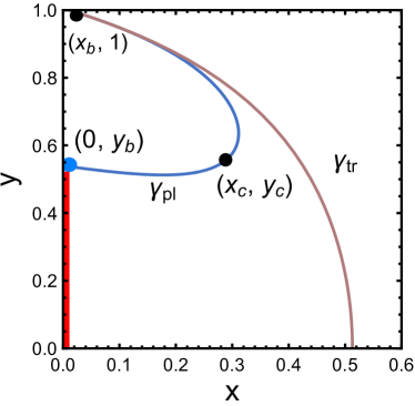
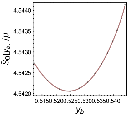
Figure 7: (a): For $\{\theta,T_{h}/\mu,\lambda,x_{b}\}=\{\pi/4,0.19894,1,\frac{1}{100}\}$, the surface penetrating the horizon $\gamma_{tr}$ is colored in rose gold, while the surface anchored on the brane $\gamma_{pl}$ and the corresponding contribution of the DGP term are colored in blue. Both of them are anchored at $x=x_{b}$ on the conformal boundary, while the half of island at $t=0$ is colored in red. (b): For $\{\theta,T_{h}/\mu,\lambda,x_{b}\}=\{\pi/4,0.19894,1,\frac{1}{100}\}$, the density difference between two surfaces is plotted as a function of $y_{b}$, by which the entropy density difference $\tilde{S}_{0}/\mu$ can be figured out as the minimum, with $\tilde{S}_{0}/\mu\approx 4.54206$.

As for the surface $\gamma_{pl}$ at $t=0$, we also introduce two different parameterizations in different intervals. In $(x,y)$ plane, for the curve in $y\in[y_{c},1]$ – see Fig. 7, we introduce $x=x(y)$ just as the parameterization of the trivial surface $\gamma_{tr}$, while for the curve in $x\in[x_{c},1]$, we introduce $y=y(x)$ instead, with $y^{\prime}(x_{c})=x^{\prime}(y_{c})^{-1}$. Finally, the density associated with the surface $\gamma_{pl}$ anchored at $y_{b}=y(0)$ can be read off from the integration procedure, with the following expressions

$$\tilde{S}_{pl}(y_{b})= \int_{y_{c}}^{1}\frac{dy}{\left(1-y^{2}\right)^{2}}\sqrt{Q_{5}\left(\frac{4Q_{2}}{P(y)}+\frac{Q_{4}\left(2y(x(y)-1)^{2}Q_{3}+x^{\prime}(y)\right)^{2}}{(x(y)-1)^{4}}\right)}+\int_{0}^{x_{c}}\frac{dx}{\left(y(x)^{2}-1\right)^{2}}$$

$$\sqrt{Q_{5}\left(\frac{4Q_{2}y^{\prime}(x)^{2}}{P(y(x))}+Q_{4}\left(4Q_{3}^{2}y(x)^{2}y^{\prime}(x)^{2}+\frac{4Q_{3}y(x)y^{\prime}(x)}{(x-1)^{2}}+\frac{1}{(x-1)^{4}}\right)\right)},$$ (51)

$$\tilde{S}_{{}_{DGP}}(y_{b})= \frac{\lambda\sqrt{Q_{5}}}{1-y_{b}^{2}}\Big{|}_{x=0},\quad y_{b}=y(0).$$ (52)

Notice that varying $(x_{c},y_{c})$ will subsequently change $y_{b}$. Thus $\tilde{S}_{pl}(y_{b})$ also depends on $y_{b}$.

The density difference between the surface $\gamma_{tr}$ and the surface $\gamma_{pl}$ with the DGP contribution is given by

$$\tilde{S}_{0}[y_{b}]=2\left(\tilde{S}_{pl}(y_{b})+\tilde{S}_{DGP}(y_{b})-\tilde{S}_{tr}(0)\right).$$ (53)

Then the corresponding entropy density difference between two candidates at $t=0$ is obtained by extremizing the above equation, which is

$$\tilde{S}_{0}=\tilde{S}_{0}[y_{{}_{QES}}]=\mathop{\text{ext}}\limits_{y_{b}}\tilde{S}_{0}[y_{b}],$$ (54)

where $\tilde{S}_{0}[y_{b}]$ reaches it extremum at $y_{b}=y_{{}_{QES}}$. The whole process is illustrated in Fig. 7.

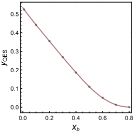
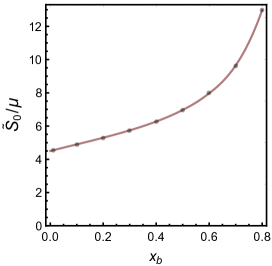
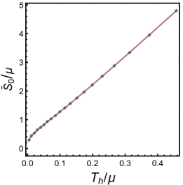
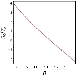
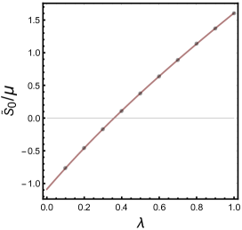
Figure 8: (a) The location of QES $y_{{}_{QES}}$ as a function of $x_{b}$, where $\{\theta,T_{h}/\mu,\lambda\}=\{\pi/4,0.19894,1\}$. (b) For $\{\theta,T_{h}/\mu,\lambda\}=\{\pi/4,0.19894,1\}$, the relation between the density difference $\tilde{S}_{0}/\mu$ and the endpoint $x_{b}$ is plotted as the solid curve. (c) For $x_{b}=1/100$, the relation between the density difference $\tilde{S}_{0}/\mu$ and $T_{h}/\mu$ is plotted as the solid curve. (d) For $\{d,\mu/T_{h},\lambda,x_{b}\}=\{3,0,0,1/5\}$, the relation between the density difference $\tilde{S}_{0}/T_{h}$ and $\theta$. (e) For $\{d,\theta,T_{h}/\mu,x_{b}\}=\{3,\pi/2,0.19894,1/5\}$, the relation between the density difference $\tilde{S}_{0}/\mu$ and the DGP coupling $\lambda$.

In Fig. 7, the difference $\tilde{S}_{0}/\mu$ is positive at $y_{{}_{QES}}\approx 0.524$. Therefore, the QES at $t=0$ is the trivial surface $\gamma_{tr}$. As Hawking radiation continues, the entanglement entropy keeps growing until Page time $t_{P}$. Then, the surface $\gamma_{pl}$ dominates at $t=t_{P}$ and the entropy saturates due to the phase transition. After Page time, the island solution dominates and the island $\mathcal{I}$ emerges in the entanglement wedge of the radiation subsystem. Therefore, the d.o.f. on the island are encoded in the radiation subsystem by quantum error correction process.

Similar to result as obtained in Sec. 3, the island will stretch out of the horizon, as illustrated in Fig. 8. It indicates that the region beyond the horizon will also be encoded in the radiation subsystem by the entanglement wedge. Furthermore, the entropy density difference $\tilde{S}_{0}/\mu$ also increases with the endpoint $x_{b}$, which is plotted in Fig. 8.

Moreover, $\tilde{S}_{0}/\mu$ increases with Hawking temperature $T_{h}/\mu$ as well, which manifests that the growth of temperature allows more entanglement to be built up between the black hole and radiation subsystem, as shown in Fig. 8.

In comparison with picture in the weak tension limit, taking the backreaction into account leads to the following significant changes. The first is that for $x_{b}\rightarrow 0$, the location of $y_{{}_{QES}}$ approaches $0.52$ – see Fig. 8, which indicates that only the region near the horizon ($0<y<y_{{}_{QES}}$) is likely to be encoded in the radiation subsystem. The second is that for $x_{b}\rightarrow 0$, the density difference $\tilde{S}_{0}/\mu$ remains positive, which clearly demonstrate that the Page curve can always be obtained, as long as the tension as well as the coupling is large enough.

Moreover, we remark that two strategies of increasing the difference of entropy density work independently, which are illustrated in Fig. 8 and Fig. 8. For the first, one may decrease $\theta$ from $\pi/2$ to $0$ but fix $\lambda=0$, then with more tension on the brane, the density difference will turn to positive and the entropy starts to evolve. Alternatively one may increase the DGP coupling $\lambda$ but fix $\theta=\pi/2$, the density difference will also turn from negative to positive.

5 Conclusions and Discussions

In this paper, we have investigated the black hole information paradox in the doubly-holographic setup for charged black holes in general dimensions. In this setup, the holographic dual of a two-sided black hole is in equilibrium with baths such that the geometry keeps stationary during the evaporation.

In the weak tension limit, we have analytically calculated the entropy of the radiation by figuring out the quantum extremal surface. With appropriate choice of the endpoint of the HRT surface, the Page curve has successfully been obtained with the presence of an island on the brane. The Page time is evaluated as well. For the neutral background in general $(d+1)$ dimensions, the entropy grows linearly at the rate proportional to $T_{h}^{d-1}$ due to the evaporation and finally saturates at a constant which depends on the size of the radiation system, while for the near-extremal case in general $(d+1)$ dimensions, the entropy grows linearly at the rate proportional to $T_{h}$. Specifically, in $4D$ charged case, we have plotted the Page curves under different temperatures. At high temperatures, the black hole seems to “evaporate” more rapidly than the cold one and will build more entanglement with the radiation. While for the near-extremal black hole, the evolution seems to be frozen, since the exchanging of Hawking modes takes place extremely slowly.

It should be noticed that in the weak tension limit, to guarantee that the difference of entropy density $\tilde{S}_{0}$ is positive, one has to choose the endpoint of the HRT surface away from the brane. As a matter of fact, such a choice transfers d.o.f. from baths to the black hole subsystem, leading to the fact that the entanglement between two subsystems is mainly contributed from the CFT matter fields.

Keep going further, we have obtained the stationary solution with backreaction by the standard DeTurck trick. Rather than transferring d.o.f. from baths, we have proposed two strategies to avoid the saturation of entropy at initial time. One is increasing the tension on the brane and another is introducing an intrinsic curvature term on the brane. Both increasing the DGP coupling $\lambda$ and decreasing the angle $\theta$ will relatively enlarge the central charge of the $(d-1)$-dimensional conformal defect, which is dual to the brane theory. Therefore, these two prescriptions are equivalent to enhancing the d.o.f. on the brane directly and hence, are more appropriate to address the information paradox for black holes. As a result, the Page curve can always be recovered, as long as the tension $\alpha$ or the DGP coupling $\lambda$ is large enough.

Next it is very desirable to investigate the time evolution of the entanglement entropy with backreaction, which involves in both more d.o.f. on the brane and the dynamics of black holes, thus beyond the DeTurck method. Furthermore, beyond the simple model with doubly-holographic setup, the information paradox for high-dimensional evaporating black holes is more complicated and difficult to describe. Therefore, it is quite interesting to develop new methods to explore the evaporation of black holes in holographic approach.

References

- [1] Don N. Page. Information in black hole radiation. Phys. Rev. Lett., 71:3743–3746, 1993.
- [2] Don N. Page. Hawking radiation and black hole thermodynamics. New J. Phys., 7:203, 2005.
- [3] Don N. Page. Time Dependence of Hawking Radiation Entropy. JCAP, 09:028, 2013.
- [4] Stephen W Hawking. Black hole explosions? Nature, 248(5443):30–31, 1974.
- [5] Ahmed Almheiri, Donald Marolf, Joseph Polchinski, and James Sully. Black Holes: Complementarity or Firewalls? JHEP, 02:062, 2013.
- [6] Juan Maldacena and Leonard Susskind. Cool horizons for entangled black holes. Fortsch. Phys., 61:781–811, 2013.
- [7] Ahmed Almheiri. Holographic Quantum Error Correction and the Projected Black Hole Interior. 10 2018.
- [8] Geoffrey Penington. Entanglement Wedge Reconstruction and the Information Paradox. 5 2019.
- [9] Ahmed Almheiri, Netta Engelhardt, Donald Marolf, and Henry Maxfield. The entropy of bulk quantum fields and the entanglement wedge of an evaporating black hole. JHEP, 12:063, 2019.
- [10] Shinsei Ryu and Tadashi Takayanagi. Holographic derivation of entanglement entropy from AdS/CFT. Phys. Rev. Lett., 96:181602, 2006.
- [11] Aitor Lewkowycz and Juan Maldacena. Generalized gravitational entropy. JHEP, 08:090, 2013.
- [12] Netta Engelhardt and Aron C. Wall. Quantum Extremal Surfaces: Holographic Entanglement Entropy beyond the Classical Regime. JHEP, 01:073, 2015.
- [13] Ahmed Almheiri, Raghu Mahajan, Juan Maldacena, and Ying Zhao. The Page curve of Hawking radiation from semiclassical geometry. JHEP, 03:149, 2020.
- [14] Hong Zhe Chen, Zachary Fisher, Juan Hernandez, Robert C. Myers, and Shan-Ming Ruan. Information Flow in Black Hole Evaporation. JHEP, 03:152, 2020.
- [15] Yiming Chen. Pulling Out the Island with Modular Flow. JHEP, 03:033, 2020.
- [16] Vijay Balasubramanian, Arjun Kar, Onkar Parrikar, Gábor Sárosi, and Tomonori Ugajin. Geometric secret sharing in a model of Hawking radiation. 3 2020.
- [17] Koji Hashimoto, Norihiro Iizuka, and Yoshinori Matsuo. Islands in Schwarzschild black holes. JHEP, 06:085, 2020.
- [18] Chethan Krishnan. Critical Islands. 7 2020.
- [19] Ahmed Almheiri, Thomas Hartman, Juan Maldacena, Edgar Shaghoulian, and Amirhossein Tajdini. The entropy of Hawking radiation. 6 2020.
- [20] Mohsen Alishahiha, Amin Faraji Astaneh, and Ali Naseh. Island in the Presence of Higher Derivative Terms. 5 2020.
- [21] Fridrik Freyr Gautason, Lukas Schneiderbauer, Watse Sybesma, and L’arus Thorlacius. Page Curve for an Evaporating Black Hole. JHEP, 05:091, 2020.
- [22] Ahmed Almheiri, Raghu Mahajan, and Juan Maldacena. Islands outside the horizon. 10 2019.
- [23] Geoff Penington, Stephen H. Shenker, Douglas Stanford, and Zhenbin Yang. Replica wormholes and the black hole interior. 11 2019.
- [24] Ahmed Almheiri, Thomas Hartman, Juan Maldacena, Edgar Shaghoulian, and Amirhossein Tajdini. Replica Wormholes and the Entropy of Hawking Radiation. JHEP, 05:013, 2020.
- [25] Ahmed Almheiri, Raghu Mahajan, and Jorge E. Santos. Entanglement islands in higher dimensions. SciPost Phys., 9(1):001, 2020.
- [26] Hao Geng and Andreas Karch. Massive Islands. 6 2020.
- [27] Hong Zhe Chen, Robert C. Myers, Dominik Neuenfeld, Ignacio A. Reyes, and Joshua Sandor. Quantum Extremal Islands Made Easy, Part I: Entanglement on the Brane. JHEP, 10:166, 2020.
- [28] Hong Zhe Chen, Robert C. Myers, Dominik Neuenfeld, Ignacio A. Reyes, and Joshua Sandor. Quantum Extremal Islands Made Easy, Part II: Black Holes on the Brane. JHEP, 12:025, 2020.
- [29] Juan Hernandez, Robert C. Myers, and Shan-Ming Ruan. Quantum Extremal Islands Made Easy, PartIII: Complexity on the Brane. 10 2020.
- [30] Ibrahim Akal, Yuya Kusuki, Tadashi Takayanagi, and Zixia Wei. Codimension two holography for wedges. 7 2020.
- [31] Rong-Xin Miao. An Exact Construction of Codimension two Holography. 9 2020.
- [32] Tadashi Takayanagi. Holographic Dual of BCFT. Phys. Rev. Lett., 107:101602, 2011.
- [33] Chong-Sun Chu and Rong-Xin Miao. Anomalous Transport in Holographic Boundary Conformal Field Theories. JHEP, 07:005, 2018.
- [34] Rong-Xin Miao. Holographic BCFT with Dirichlet Boundary Condition. JHEP, 02:025, 2019.
- [35] Matthew Headrick, Sam Kitchen, and Toby Wiseman. A New approach to static numerical relativity, and its application to Kaluza-Klein black holes. Class. Quant. Grav., 27:035002, 2010.
- [36] Óscar J.C. Dias, Jorge E. Santos, and Benson Way. Numerical Methods for Finding Stationary Gravitational Solutions. Class. Quant. Grav., 33(13):133001, 2016.
- [37] Hao Geng, Andreas Karch, Carlos Perez-Pardavila, Suvrat Raju, Lisa Randall, Marcos Riojas, and Sanjit Shashi. Information Transfer with a Gravitating Bath. 12 2020.
- [38] Lisa Randall and Raman Sundrum. An Alternative to compactification. Phys. Rev. Lett., 83:4690–4693, 1999.
- [39] G.R. Dvali, Gregory Gabadadze, and Massimo Porrati. 4-D gravity on a brane in 5-D Minkowski space. Phys. Lett. B, 485:208–214, 2000.
- [40] Andreas Karch and Lisa Randall. Locally localized gravity. JHEP, 05:008, 2001.
- [41] Masahiro Nozaki, Tadashi Takayanagi, and Tomonori Ugajin. Central Charges for BCFTs and Holography. JHEP, 06:066, 2012.
- [42] Thomas Hartman and Juan Maldacena. Time Evolution of Entanglement Entropy from Black Hole Interiors. JHEP, 05:014, 2013.
- [43] Dean Carmi, Shira Chapman, Hugo Marrochio, Robert C. Myers, and Sotaro Sugishita. On the Time Dependence of Holographic Complexity. JHEP, 11:188, 2017.