The environmental dependence of the $X_{\mathrm{CO}}$ conversion factor

Abstract

$\mathrm{CO}$ is the most widely used observational tracer of molecular gas. The observable $\mathrm{CO}$ luminosity is translated to $\mathrm{H_{2}}$ mass via a conversion factor, $X_{\mathrm{CO}}$, which is a source of uncertainty and bias. Despite variations in $X_{\mathrm{CO}}$, the empirically-determined solar neighborhood value is often applied across different galactic environments. To improve understanding of $X_{\mathrm{CO}}$, we employ 3D magnetohydrodynamics simulations of the interstellar medium (ISM) in galactic disks with a large range of gas surface densities, allowing for varying metallicity, far-ultraviolet (FUV) radiation, and cosmic ray ionization rate (CRIR). With the TIGRESS simulation framework we model the three-phase ISM with self-consistent star formation and feedback, and post-process outputs with chemistry and radiation transfer to generate synthetic CO(1–0) and (2–1) maps. Our models reproduce the observed CO excitation temperatures, line-widths, and line ratios in nearby disk galaxies. $X_{\mathrm{CO}}$ decreases with increasing metallicity, with a power-law slope of $-0.8$ for the (1–0) line and $-0.5$ for the (2–1) line. $X_{\mathrm{CO}}$ also decreases at higher CRIR, and is insensitive to the FUV radiation. As density increases, $X_{\mathrm{CO}}$ first decreases due to increasing excitation temperature, and then increases when the emission is fully saturated. We provide fits between $X_{\mathrm{CO}}$ and observable quantities such as the line ratio, peak antenna temperature, and line brightness, which probe local gas conditions. These fits, which allow for varying beam size, may be used in observations to calibrate out systematic biases. We also provide estimates of the CO-dark $\mathrm{H_{2}}$ fraction at different gas surface densities, observational sensitivities, and beam sizes.

1. Introduction

Molecular clouds are the cradles for star formation in galaxies. Measuring the total molecular content as well as the distribution and properties of molecular clouds is therefore crucial to empirical characterization of star formation itself and of the energy returned by massive young stars to the ISM. Although $\mathrm{H_{2}}$ is the most abundant molecule in the ISM, it is difficult to observe in emission due to its low mass and lack of dipole moment. As a result, the second most abundant molecule, $\mathrm{CO}$, is often used to trace $\mathrm{H_{2}}$. However, $\mathrm{CO}$ emission is usually optically thick, and the standard technique relies on applying a conversion factor to translate the observed $\mathrm{CO}$ line brightness $W_{\mathrm{CO}}$ to the column density of molecular hydrogen $N_{\mathrm{H_{2}}}$,

$$X_{\mathrm{CO}}\equiv\frac{N_{\mathrm{H_{2}}}}{W_{\mathrm{CO}}}.$$ (1)

Equivalently, the total molecular gas mass surface density (including helium) is obtained as $\Sigma_{\mathrm{mol}}=\alpha_{\mathrm{CO}}W_{\mathrm{CO}}$ using a conversion factor $\alpha_{\mathrm{CO}}=2.8m_{p}X_{\mathrm{CO}}$.

Traditionally, $X_{\mathrm{CO}}$ is defined for emission in the $J=1-0$ rotational transition (hereafter denoted as (1–0)). It can be measured empirically by determining the $\mathrm{H_{2}}$ mass using dust emission or extinction, gamma-ray emission, or the virial theorem (e.g. Dame et al. 2001; Lombardi et al. 2006; Strong & Mattox 1996; Solomon et al. 1987). The average value of $X_{\mathrm{CO}}$ in the Milky Way solar neighborhood is $X_{\mathrm{CO,MW}}=2\times 10^{20}~{}\mathrm{cm^{-2}K^{-1}km^{-1}s}$, corresponding to $\alpha_{\mathrm{CO,MW}}=4.3~{}M_{\odot}\mathrm{pc^{-2}K^{-1}km^{-1}s}$ (see review by Bolatto et al. 2013). Often, values of $X_{\mathrm{CO,20}}\equiv X_{\mathrm{CO}}/(10^{20}~{}\mathrm{cm^{-2}K^{-1}km^{-1}s})$ are reported, and we will adopt this shorthand for numerical results.

Recently, interferometers such as ALMA have enabled high resolution observations in nearby galaxies, revealing unprecedented details of molecular clouds in a wide range of environments down to scales of tens of parsecs (e.g. Schinnerer et al. 2013; Leroy et al. 2016; Egusa et al. 2018; Faesi et al. 2018; Sun et al. 2018, 2020). However, the environmental dependence of $X_{\mathrm{CO}}$ is not well understood, and can introduce significant uncertainties and biases in measuring the mass and pressure of molecular gas (Sun et al. 2020). In addition, many observations are conducted using the CO(2–1) line in order to achieve higher resolution, and often a fixed ratio of the (2–1)/(1–0) line intensity is adopted in order to estimate $X_{\mathrm{CO}}$ (Gratier et al. 2010; Sun et al. 2020).

The uncertainties in $X_{\mathrm{CO}}$ stem from the fact that the value of $X_{\mathrm{CO}}$ is observed to vary both locally on small scales within individual molecular clouds where the volume and column density as well as thermal and turbulent motions vary (e.g. Solomon et al. 1987; Pineda et al. 2008; Ripple et al. 2013; Kong et al. 2015); and on large scales across galaxies where the total gas surface density and velocity dispersion as well as environmental conditions such as the metallicity and gas heating rate are nonuniform (e.g. Israel 1997; Downes & Solomon 1998; Leroy et al. 2011; Sandstrom et al. 2013; Bolatto et al. 2013). To make the most of the new molecular observations, it is essential to understand and calibrate the variations in $X_{\mathrm{CO}}$.

Many efforts have been made to investigate $X_{\mathrm{CO}}$ using theoretical models. The approach in Wolfire et al. (2010) combines the comprehensive chemical network of a photodissociation region (PDR) code with a highly simplified spherical cloud model. Accurso et al. (2017) further coupled radiation from stellar populations to similar spherical cloud models. These studies both allow for comprehensive chemical networks, but lack the realistic density and velocity structure produced by turbulence in molecular clouds and their environments To model more realistic, turbulent molecular clouds, several studies have employed 3D numerical hydrodynamic and magnetohydrodynamic (MHD) simulations to investigate $X_{\mathrm{CO}}$ (e.g. Glover & Mac Low 2011; Shetty et al. 2011a, b; Glover & Clark 2012; Szűcs et al. 2016). The molecular clouds in these simulations are modeled in domains with sizes from parsec to tens of parsecs, and are effectively isolated from the galactic ISM. Their physical properties such as the density, cloud size, and velocity structure are set by hand via initial conditions and turbulent driving specified in the simulations, and radiation fields impinging on the cloud must also be specified by hand. At the other extreme, galaxy simulations have also been used to explore variations in $X_{\mathrm{CO}}$ (e.g Narayanan et al. 2011, 2012; Feldmann et al. 2012; Duarte-Cabral et al. 2015; Li et al. 2018). These models can capture global environmental variations, but with resolutions coarser than tens of parsecs individual molecular clouds are not resolved, and sub-grid models are required to estimate the $\mathrm{CO}$ brightness. Due to the computational cost limitations, most of these cloud- and galaxy-scale simulations obtain the chemical abundances of $\mathrm{H_{2}}$ and $\mathrm{CO}$ from either sub-grid models that assume a simplified PDR-like structure within each grid cell or simplified chemistry networks such as those from Nelson & Langer (1997) and Nelson & Langer (1999).

In our previous work (Gong et al. 2018, hereafter GOK2018), we investigated $X_{\mathrm{CO}}$ using local galactic disk MHD simulations where massive clouds are formed self-consistently in the three-phase ISM with star formation and feedback. We modeled the chemical abundances in post-processing with a compact network described in Gong et al. (2017), which included significant improvements over Nelson & Langer (1999) and demonstrated good agreement with the comprehensive PDR code in Wolfire et al. (2010). For this study, kpc-scale conditions input to the MHD simulations were similar to the solar neighborhood environment, and evolution of the ISM covered more than a full star formation cycle ($\sim 50\mathrm{Myr}$) at pc-scale resolution (Kim & Ostriker 2017, hereafter KO2017). This study demonstrated that a mean $X_{\mathrm{CO}}\approx 0.7-2\times 10^{20}~{}\mathrm{cm^{-2}K^{-1}km^{-1}s}$ is obtained (varying somewhat in time and increasing for large beams), in agreement with Milky Way observations. It also showed that $W_{\mathrm{CO}}$ is sensitive to density, since collisions are what determines the excitation of rotational transitions. Starting from similar local galactic disk models with solar neighborhood-like parameters (Walch et al. 2015), Seifried et al. (2017, 2020) performed zoom-in simulations of giant molecular clouds (GMCs) with time-dependent chemistry using the Nelson & Langer (1997) network, and achieved a resolution of 0.1 pc. They obtained typical $X_{\mathrm{CO}}\approx 1.5\times 10^{20}~{}\mathrm{cm^{-2}K^{-1}km^{-1}s}$ for a few GMCs, again in agreement with observations. Both of these recent studies emphasized that $X_{\mathrm{CO}}$ has considerable scatter on small scales. Local-box simulations of this kind are particularly advantageous for investigating $X_{\mathrm{CO}}$, because they include enough physics to produce a realistic ISM, while also having high resolution. However, to date only solar neighborhood conditions have been considered, not yet addressing potentially important environmentally-driven variations in $X_{\mathrm{CO}}$, such as the dependence on metallicity (Bolatto et al. 2013). Moreover, theoretical models so far have mostly focused on the CO(1–0) line, although the (2–1) line has been used increasingly in observations (e.g. Sun et al. 2018).

In this paper, we build upon GOK2018 to study and calibrate $X_{\mathrm{CO}}$ more comprehensively, covering a range of ISM conditions that prevail in local-Universe galaxies. As before, we perform 3D MHD simulations of kpc-sized regions of galactic disks with $\sim$pc resolution, which produces clouds with realistic density and velocity structure as determined by self-gravity and turbulence driven naturally by star formation feedback. The $\mathrm{H_{2}}$ and $\mathrm{CO}$ abundances and CO(1–0) and (2–1) line emission maps are obtained via chemistry and radiation transfer post-processing. By varying the initial large-scale surface density in the MHD simulations, as well as the metallicity, the far ultraviolet (FUV) radiation field strength, and the cosmic ray ionization rate (CRIR) in the post-processing, we systematically investigate the dependence of $X_{\mathrm{CO}}$ on these environmental parameters. We also study the effect of beam sizes in our synthetic observations. We analyze how and why $X_{\mathrm{CO}}$ depends on large-scale and small-scale environmental conditions. We also quantify the dependence of $X_{\mathrm{CO}}$ on direct observables (total CO(1–0) and (2–1) line strength, peak antenna temperature, and line ratio) that probe gas conditions for different models, at a range of observational beam sizes. Based on the correlations we identify, we provide formulae to calibrate $X_{\mathrm{CO}}$; these calibrations can be used to reduce systematic biases that enter if a constant $X_{\mathrm{CO}}$ is adopted to convert observed $W_{\mathrm{CO}}$ to $N_{\mathrm{H_{2}}}$. The present work may be seen as a natural extension of GOK2018 beyond solar neighborhood environments.

The structure of this paper is as follows. In Section 2, we use simple theoretical models to explain the physics that enters in setting $X_{\mathrm{CO}}$; this provides insight into the environmental dependencies that may be expected. In Section 3, we describe the methods adopted for our numerical MHD simulations, and the post-processing chemistry and radiative transfer that we use to produce synthetic observations. Our results are presented in Section 4: first, we describe the overall properties of the simulations in Section 4.1; then we validate our simulations by comparing with observations in Section 4.2; Section 4.3 investigates the dependence of $X_{\mathrm{CO}}$ on environmental and observable parameters and provides calibration formulae for $X_{\mathrm{CO}}$; lastly, Section 4.4 quantifies the variations in the CO-dark $\mathrm{H_{2}}$ fraction. Finally, we summarize our conclusions in Section 5.

2. Theoretical Expectations

Although the definition of $X_{\mathrm{CO}}=N_{\mathrm{H_{2}}}/W_{\mathrm{CO}}$ is simple, both $N_{\mathrm{H_{2}}}$ and $W_{\mathrm{CO}}$ have complex dependencies on many physical parameters. For example, the cloud density structure influences where both $\mathrm{CO}$ and $\mathrm{H_{2}}$ form. The gas kinetic temperature affects collision rates and hence the population of $\mathrm{CO}$ rotational energy levels and transition rates. The velocity structure affects how much $\mathrm{CO}$ emission can escape the optically thick dense gas and thus the brightness of the $\mathrm{CO}$ line. The metallicity changes the formation rate of $\mathrm{H_{2}}$ and amount of dust shielding available. The external FUV radiation and CR ionization hinder formation of molecules, while also setting the gas heating rate. Due to these complex factors, it is difficult to make an accurate analytical prediction of $X_{\mathrm{CO}}$ as a simple function of the environmental variables. However, reference to simple models is still quite useful for providing insights into what $X_{\mathrm{CO}}$ may depend on, and in which direction.

Typically, $\mathrm{CO}$ line profiles are not too far from Gaussian, and to the first order, $W_{\mathrm{CO}}\propto\sigma_{v}T_{\mathrm{peak}}$, where $\sigma_{v}$ is the width of the line and $T_{\mathrm{peak}}$ is the peak antenna temperature. From Section 3.1.2 in GOK2018, for a uniform slab with optically thick $\mathrm{CO}$ emission and $T_{\mathrm{peak}}\gtrsim 5.5~{}\mathrm{K}$, $T_{\mathrm{peak}}\approx T_{\mathrm{exc}}$ where $T_{\mathrm{exc}}$ is the excitation temperature of the line. Thus, we can approximate $X_{\mathrm{CO}}$ as

$$X_{\mathrm{CO}}\equiv\frac{N_{\mathrm{H_{2}}}}{W_{\mathrm{CO}}}\sim\frac{N_{\mathrm{H_{2}}}}{\sigma_{v}T_{\mathrm{exc}}}\sim\frac{N_{\mathrm{H_{2}}}/n}{\sigma_{v}(T_{\mathrm{exc}}/n)}.$$ (2)

where $n$ is the number density of hydrogen atoms. The factor in the numerator, $N_{\mathrm{H_{2}}}/n$ is determined by the $\mathrm{H_{2}}$ formation chemistry, and by the turbulent structure of the molecular clouds. GOK2018 pointed out that $\sigma_{v}$ does not vary as much as $T_{\mathrm{exc}}$, so in the denominator the factor $T_{\mathrm{exc}}/n$ is more important for $X_{\mathrm{CO}}$.

We can make the further assumption that the molecular gas is either (1) in clouds in approximate virial equilibrium with mean density $\rho$ and size $L_{\mathrm{cloud}}\sim\sigma_{v}/\sqrt{G\rho}$, or (2) dominating the mass in the galactic midplane of an ISM disk that is in vertical equilibrium, with scale height $H\sim\sigma_{v}^{2}/(G\Sigma_{\mathrm{H_{2}}})$. In either case, $N_{\mathrm{H_{2}}}\propto\sigma_{v}\sqrt{n}$, which gives

$$X_{\mathrm{CO}}\propto\frac{\sqrt{n}}{T_{\mathrm{exc}}}.$$ (3)

Taking the CO(1–0) as an example and using a simplified two-level system model,

$$\frac{1}{T_{\mathrm{exc}}}=\frac{1}{T_{\mathrm{gas}}}+\frac{1}{T_{0}}\ln\left(1+\frac{\beta A_{10}}{n_{c}k_{10}}\right)\approx\frac{1}{T_{\mathrm{gas}}}+\frac{\beta A_{10}}{n_{c}k_{10}T_{0}}$$ (4)

from Equation (30) in GOK2018. Here, $T_{\mathrm{gas}}$ is the gas temperature, $n_{c}$ is the density of the collisional partner ($\mathrm{H_{2}}$ in this case), $\beta=(1-e^{-\tau})/\tau$ is the escape probability of the line, $\tau$ is the optical depth of the line, $k_{10}\approx 6\times 10^{-11}(T_{\mathrm{gas}}/100~{}\mathrm{K})^{0.2}~{}\mathrm{cm^{3}s^{-1}}$ is the collisional de-excitation rate, $T_{0}=5.5~{}\mathrm{K}$ characterizes the transition energy and $A_{10}=7.203\times 10^{-8}~{}\mathrm{s^{-1}}$ is the Einstein A coefficient. If the optical depth $\tau\gg 1$, $\beta\approx 1/\tau$. The expansion of the logarithm is generally valid for the conditions in molecular clouds, where $n_{c}\gtrsim 50\,\mathrm{cm}^{-3}$, $T_{\mathrm{gas}}\sim 10-100$K, and $\tau\gtrsim 10$.

Using the large velocity gradient (LVG) approximation, the optical depth is (Equation (7) in GOK2018)

$$\tau_{\mathrm{LVG}}=\frac{\lambda_{10}^{3}}{8\pi}\frac{A_{10}n_{\mathrm{CO}}}{|\mathrm{d}v/\mathrm{d}r|}f_{1}\left(\frac{f_{0}/g_{0}}{f_{1}/g_{1}}-1\right),$$ (5)

where $\lambda_{10}=2.6\,{\rm mm}$, $n_{\mathrm{CO}}$ is the number density of $\mathrm{CO}$ molecules, $g_{0}=1$ and $g_{1}=3$ are the degeneracies for $J=0$ and $J=1$ levels, $f_{0}=n_{0}/n_{\mathrm{CO}}$ and $f_{1}=n_{1}/n_{\mathrm{CO}}$ are the fractions of $\mathrm{CO}$ molecules in $J=0$ and $J=1$ levels, $n_{0}$ and $n_{1}$ are the level populations, and $|\mathrm{d}v/\mathrm{d}r|$ is the velocity gradient. If $T_{\mathrm{exc}}\gtrsim T_{0}$, with the definition of $T_{\mathrm{exc}}\equiv T_{0}/\ln[(f_{0}/g_{0})/(f_{1}/g_{1})]$ and $f_{0}+f_{1}=1$, then to the first order of ($T_{0}/T_{\mathrm{exc}}$),

$$f_{1}\left(\frac{f_{0}/g_{0}}{f_{1}/g_{1}}-1\right)=\frac{e^{T_{0}/T_{\mathrm{exc}}}-1}{1+\frac{g_{0}}{g_{1}}e^{T_{0}/T_{\mathrm{exc}}}}\approx\left(1-\frac{g_{0}}{g_{1}}\right)\frac{T_{0}}{T_{\mathrm{exc}}}.$$ (6)

This then gives

$$\frac{\beta A_{10}}{n_{c}k_{10}}\approx\frac{24\pi}{k_{10}\lambda_{10}^{3}}\frac{|\mathrm{d}v/\mathrm{d}r|}{n^{2}f_{\mathrm{CO}}}\frac{T_{\mathrm{exc}}}{T_{0}},$$ (7)

assuming $n_{c}=n_{\mathrm{H_{2}}}\approx 0.5n$ in $\mathrm{CO}$ dominated regions; $f_{\mathrm{CO}}=n_{\mathrm{CO}}/n$ is the CO abundance relative to hydrogen.

We consider two limits from Equations (3), (4) and (7). In the first case, we consider relatively low $n$. In this case, $\beta A_{10}/(n_{c}k_{10})$ is relatively large (while still allowing the logarithm to be expanded to lowest order), and the second term on the right-hand side of Equation (4) dominates. Equation (4) then gives $\beta A_{10}/(n_{c}k_{10})\approx T_{0}/T_{\mathrm{exc}}$, and when combined with Equation (7) this yields

$$T_{\mathrm{exc}}\propto n\left(\frac{f_{\mathrm{CO}}}{|\mathrm{d}v/\mathrm{d}r|}\right)^{1/2}.$$ (8)

Finally, inserting in Equation (3) we obtain for the low-density limit

$$X_{\mathrm{CO}}\propto\left(\frac{|\mathrm{d}v/\mathrm{d}r|}{nf_{\mathrm{CO}}}\right)^{1/2}.$$ (9)

We find that in the simulations, $|\mathrm{d}v/\mathrm{d}r|$ has no systematic density dependence. In this case, as density and $f_{\mathrm{CO}}$ increase, $X_{\mathrm{CO}}$ decreases.

The second case we consider is when $n$ is large, so the first term in the denominator of Equation (4) dominates. This is the LTE limit of $T_{\mathrm{exc}}\to T_{\mathrm{gas}}$. In this high density limit we then have

$$X_{\mathrm{CO}}\propto\frac{\sqrt{n}}{T_{\mathrm{gas}}},$$ (10)

which increases with density. Although $T_{\mathrm{gas}}$ does not vary much within individual dense molecular clouds, it may be higher in environments with high star formation rates (SFRs) and hence high cosmic ray heating.

We note that the dependencies of $X_{\mathrm{CO}}$ for low- and high-density limits in Equations 9 and 10 are derived using over-simplified assumptions, and thus are never strictly true in realistic molecular clouds. However, they provide theoretical insight to the behavior that emerges from much more complex numerical simulations. In particular, the above arguments show that $X_{\mathrm{CO}}$ is not expected to be constant on small scales. In fact, we expect $X_{\mathrm{CO}}$ to have a non-monotonic relation with density.

On large scales, the main external environmental factors we consider in this paper are the FUV radiation field strength, the CRIR, and the metallicity $Z$. From the simple photodissociation region (PDR) models in Gong et al. (2017) (for example their Figures 5 and 6), we expect that FUV radiation destroys both $\mathrm{H_{2}}$ and $\mathrm{CO}$. The CRIR, on the other hand, also impedes both $\mathrm{H_{2}}$ and $\mathrm{CO}$ formation, but has the additional effect of heating up the molecular gas and raising the temperature in $\mathrm{CO}$ dominated regions. Therefore, we expect a larger effect on $X_{\mathrm{CO}}$ from the CRIR than from the FUV radiation. By raising $T_{\mathrm{gas}}$, which tends to increase $T_{\mathrm{exc}}$ from Equation 4, $X_{\mathrm{CO}}$ will be reduced as the CRIR increases. Equation 4 also suggests a higher $X_{\mathrm{CO}}$ at lower metallicity $Z$, where $f_{\mathrm{CO}}$ decreases due to lower carbon and oxygen abundances and lower shielding.

Another important observational parameter is $f_{\mathrm{dark}}$, the fraction of $\mathrm{CO}$-dark $\mathrm{H_{2}}$. This is defined as the fraction of $\mathrm{H_{2}}$ with $\mathrm{CO}$ emission below some detection limit $W_{\mathrm{CO,det}}$,

$$f_{\mathrm{dark}}=\frac{M_{\mathrm{H_{2}}}(W_{\mathrm{CO}}<W_{\mathrm{CO,det}})}{M_{\mathrm{H_{2},tot}}}.$$ (11)

Evidently, $f_{\mathrm{dark}}$ increases with $W_{\mathrm{CO,det}}$. We adopt a constant $W_{\mathrm{CO,det}}$ similar to the PHANGS observations in the main part of this paper (see Section 3.2), and further discuss the relation between $f_{\mathrm{dark}}$ and $W_{\mathrm{CO,det}}$ in Section 4.4.

3. Methods

The methods used here are very similar to those in GOK2018, but are extended to apply to environments beyond the solar neighborhood. We post-process simulations of galactic disks with chemistry to obtain the distribution of $\mathrm{H_{2}}$ and $\mathrm{CO}$, and then use a radiation transfer code to model the $\mathrm{CO}$ line emission from molecular clouds. Below we briefly describe our methods and refer the readers to GOK2018 for more extensive descriptions.

3.1. MHD simulations

Figure 1.— Schematic illustration of the TIGRESS framework. R2, R4 and R8 models roughly represent the environments in a Milky Way-like galaxy at 2, 4, and 8 kpc from the galactic center. The gas surface density and SFR decrease from R2 to R4 to R8. Image credit: face-on galaxy NGC 3982: ESA/NASA; edge-on galaxy NGC 891: Robert Gendler, NAOJ, HST/NASA, BYU (Michael Joner, David Laney).

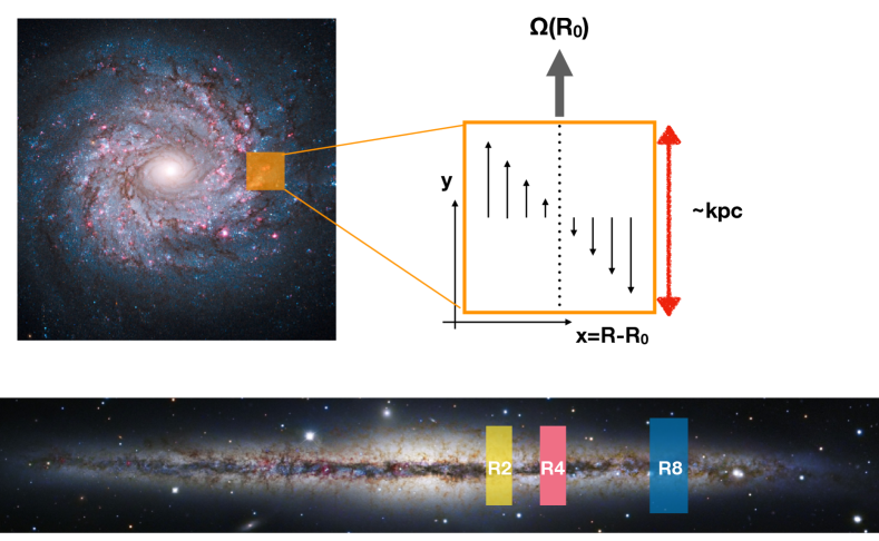
The MHD simulation is carried out with the TIGRESS (Three-phase Interstellar medium in Galaxies Resolving Evolution with Star formation and Supernova feedback) framework described by KO2017 . A schematic illustration of the TIGRESS framework is shown in Figure 1. Each simulation represents a $\sim$ kpc-sized patch of a galactic disk where the multiphase ISM is self-consistently modeled with resolved star formation and feedback. The simulations are conducted using the Athena code (Stone et al. 2008; Stone & Gardiner 2009), in a vertically-stratified local shearing box (e.g. Stone & Gardiner 2010). The ideal MHD equations are solved, including gravitational forces from gas, stars, and the dark matter halo (the old stellar disk and the dark matter halo are treated via fixed potentials). Sink particles are implemented to represent star clusters (Gong & Ostriker 2013), and produce radiation and supernova feedback to the ISM from the massive stars they contain. Only core-collapse supernovae are included, from both young star clusters and runaway stars that originated from OB binaries in clusters. The rate of SN explosions is adopted from the stellar population synthesis model STARBURST99 (Leitherer et al. 1999). The FUV radiation from massive stars uses the same stellar population synthesis model and is based on the instantaneous average luminosity per unit area over the whole simulated domain, with a simple attenuation factor to account for the mean dust optical depth. This average radiation field is used to obtain the mean heating rate in the atomic ISM (without solving the radiative transfer on-the-fly).

Each TIGRESS simulation is run for at least 1.5$t_{\mathrm{orb}}$ (corresponding to several star formation cycles), where $t_{\mathrm{orb}}=2\pi/\Omega$ is the local galactic disk orbital time. A turbulent and magnetized three-phase ISM with realistic properties emerges. Overall, quasi-steady state is reached, with periods of enhanced star formation followed by periods of enhanced feedback; feedback disperses dense gas, which recollects over time due to gravity and large-scale converging flows. No gas is added to the domain, but gas is continually lost to galactic winds (Kim & Ostriker 2018; Kim et al. 2020b, a) and to star formation, so the mean gas surface density declines over time in each simulation. Much of the volume is occupied by hot ionized gas, and most of the mass resides near the midplane in the warm and cold neutral medium (WNM and CNM), similar to the observed ISM in the Milky Way and nearby galaxies. Although molecular gas is not explicitly modeled in the time-dependent simulations, it is expected to form within the dense and shielded regions of the CNM. We model the formation of molecular gas by post-processing the simulations with chemistry and shielding, which is described in detail in Section 3.2.

Table 1Galactic Environments in Simulations

Environment	$\Sigma_{\mathrm{gas,init}}$	$\Sigma_{\mathrm{gas}}$	$\Sigma_{\mathrm{star}}$	$\rho_{\mathrm{DM}}$	$\Omega$
R2	150	40–100	450	0.08	0.1
R4	50	20–40	208	0.02	0.05
R8	12	9–11	42	0.006	0.03

We extend the solar neighborhood TIGRESS model from KO2017 (as previously analyzed in GOK2018) to a wider range of environments, as listed in Table 1 (see also Kim et al. 2020a). Three types of initial conditions are adopted and the corresponding MHD models are named R2, R4 and R8. These very roughly represent environments in a generic Milky Way-like galactic disk at radial distances of 2, 4, and 8 kpc from the galactic center (see Figure 1). All of the densities (gas, stars, and dark matter) increase from R8 to R4 to R2, closer to the notional galactic center. As a result of both high gas surface density and the strong vertical gravity from the stellar disk, the SFR increases from R8 to R4 to R2. For the R2 and R4 models, feedback drives stronger outflows than in the R8 model previously studied in GOK2018, especially in the initial stage of the simulation, leading to a larger decrease in the gas surface density in the steady state compared to the initial values. We note that because the simulations are local, the galactocentric radius does not directly enter the model specification. The suite of models can therefore equally well be thought of as spanning a range of galactic environments from low to high values of $\Sigma_{\mathrm{gas}}$ and $\Sigma_{\mathrm{star}}$, without regard to the position in a galaxy.

Table 2MHD Simulation and Post-processing Model Parameters

Model ID	Environment	$\Delta x$	$L_{\mathrm{x,y}}$	$t_{\mathrm{pp}}$	$Z$	$f_{\mathrm{CR}}$	$f_{\mathrm{FUV}}$	$\xi_{0}$	$\langle\xi\rangle_{M_{CO}}$	$\chi_{0}$
Physical environment:
R2-Z1CR10L10	R2	2	256	40–80	1	1	1	$(1.6\pm 1.1)\times 10^{-14}$	$(1.1\pm 0.6)\times 10^{-15}$	$78\pm 55$
R2-Z1L10	$\cdots$	$\cdots$	$\cdots$	$\cdots$	1	0.1	1
R2-Z1CR10	$\cdots$	$\cdots$	$\cdots$	$\cdots$	1	1	0.1
R2-Z1	$\mathbf{\cdots}$	$\mathbf{\cdots}$	$\mathbf{\cdots}$	$\mathbf{\cdots}$	1	0.1	0.1	$\mathbf{(1.6\pm 1.1)\times 10^{-15}}$	$\mathbf{(1.1\pm 0.6)\times 10^{-16}}$	$\mathbf{7.8\pm 5.5}$
R2-Z1L01	$\cdots$	$\cdots$	$\cdots$	$\cdots$	1	0.1	0.01
R2-Z1CR01	$\cdots$	$\cdots$	$\cdots$	$\cdots$	1	0.01	0.1
R2-Z1CR01L01	$\cdots$	$\cdots$	$\cdots$	$\cdots$	1	0.01	0.01
R2-Z05	$\cdots$	$\cdots$	$\cdots$	$\cdots$	0.5	0.1	0.1
R2-Z2	$\cdots$	$\cdots$	$\cdots$	$\cdots$	2	0.1	0.1
R4-Z1CR10L10	R4	2	512	50-160	1	1	1	$(5.1\pm 3.3)\times 10^{-15}$	$(5.0\pm 2.4)\times 10^{-16}$	$26\pm 16$
R4-Z1L10	$\cdots$	$\cdots$	$\cdots$	$\cdots$	1	0.1	1
R4-Z1CR10	$\cdots$	$\cdots$	$\cdots$	$\cdots$	1	1	0.1
R4-Z1	$\mathbf{\cdots}$	$\mathbf{\cdots}$	$\mathbf{\cdots}$	$\mathbf{\cdots}$	1	0.1	0.1	$\mathbf{(5.1\pm 3.3)\times 10^{-16}}$	$\mathbf{(5.0\pm 2.4)\times 10^{-17}}$	$\mathbf{2.6\pm 1.6}$
R4-Z1L01	$\cdots$	$\cdots$	$\cdots$	$\cdots$	1	0.1	0.01
R4-Z1CR01	$\cdots$	$\cdots$	$\cdots$	$\cdots$	1	0.01	0.1
R4-Z1CR01L01	$\cdots$	$\cdots$	$\cdots$	$\cdots$	1	0.01	0.01
R4-Z05	$\cdots$	$\cdots$	$\cdots$	$\cdots$	0.5	0.1	0.1
R4-Z2	$\cdots$	$\cdots$	$\cdots$	$\cdots$	2	0.1	0.1
R8-Z1	R8	2	1024	300–400	1	1	1	$\mathbf{(4.7\pm 4.0)\times 10^{-16}}$	$\mathbf{(9.2\pm 5.8)\times 10^{-17}}$	$\mathbf{2.4\pm 2.0}$
R8-Z05	$\cdots$	$\cdots$	$\cdots$	$\cdots$	0.5	1	1
R8-Z2	$\cdots$	$\cdots$	$\cdots$	$\cdots$	2	1	1
Convergence of simulation box-size:
R2B2-Z1	R2	2	512	40–60	1	0.1	0.1	$(8.2\pm 3.6)\times 10^{-15}$	$(4.9\pm 1.8)\times 10^{-16}$	$4.1\pm 1.8$
R2B2-Z05	$\cdots$	$\cdots$	$\cdots$	$\cdots$	0.5	0.1	0.1
R2B2-Z2	$\cdots$	$\cdots$	$\cdots$	$\cdots$	2	0.1	0.1
Convergence of numerical resolution
R2N2-Z1	R2	1	256	51–54	1	0.1	0.1	$(5.6\pm 1.1)\times 10^{-15}$	$(5.3\pm 1.2)\times 10^{-16}$	$2.8\pm 0.5$
R2N2-Z05	$\cdots$	$\cdots$	$\cdots$	$\cdots$	0.5	0.1	0.1
R2N2-Z2	$\cdots$	$\cdots$	$\cdots$	$\cdots$	2	0.1	0.1

The physical parameters of the TIGRESS MHD simulations are summarized as part of Table 2. The simulations are conducted using a regular Cartesian grid. Each resolution element has a size of $\Delta x$ in all three dimensions. The simulations are run with a resolution of $\Delta x=2~{}\mathrm{pc}$. In order to obtain a higher numerical resolution with limited computational resources, we restart one of the R2 simulation after it reaches the steady state (at $50~{}\mathrm{Myr}$) with a doubled resolution of $1~{}\mathrm{pc}$, and run that for $4~{}\mathrm{Myr}$. The boundary condition is shearing-periodic in the $x$ direction, periodic in the $y$ direction, and outflow in the $z$ direction. The simulation box-size is $L_{x}\times L_{y}\times L_{z}$, where $L_{x}=L_{y}$ and $L_{z}=3584~{}\mathrm{pc}$ for R2 and R4 models and $L_{z}=7168$ for R8 models. $L_{x}$ and $L_{y}$ increases from $256~{}\mathrm{pc}$ in R2 models to $1024~{}\mathrm{pc}$ in R8 models. Larger horizontal box sizes are needed in the lower surface density models, where the expanding bubbles from supernovae explosions are larger due to the lower mean density, and individual superbubbles (created by correlated supernovae explosions) can fill the whole midplane volume if the box size is too small (Kim et al. 2020a). We also carry out a set of R2 models with a larger horizontal box size of $L_{x}=L_{y}=512~{}\mathrm{pc}$ to investigate the numerical effect of the changing box sizes.

3.2. Post-processing $X_{\mathrm{CO}}$

To obtain the chemical composition of the gas, we use the chemistry post-processing module within the code Athena++ (White et al. 2016; Stone et al. 2020) that we developed in GOK2018. Because almost all mass and molecular gas resides near the midplane, we isolate the midplane region of $-512~{}\mathrm{pc}<z<512~{}\mathrm{pc}$ for post-processing. The code reads the output from the TIGRESS simulations and performs chemistry calculations assuming the density and velocity in each grid cell are fixed.

We use the simplified chemical network of Gong et al. (2017), which gives accurate abundances of $\mathrm{H_{2}}$ and $\mathrm{CO}$. In order to compute the photoionization and photodissociation rates of the chemical species, we use the six-ray approximation: in each cell, the radiation field is calculated by ray-tracing and averaged over six directions along the Cartesian axes accounting for the dust and molecular line shielding (Nelson & Langer 1997, 1999; Glover & Mac Low 2007). The incident unattenuated radiation field is assumed to come from the edge of the computational domain along each ray. The unattenuated FUV radiation is directly obtained from the TIGRESS simulations (see Section 3.1).

The CRIR is similarly calculated with the six-ray method, where $\xi(N_{\mathrm{H}})$ is computed along each ray and averaged to obtain the final value. We adapt the CR attenuation prescription of Neufeld & Wolfire (2017) and Silsbee & Ivlev (2019),

$$\xi(N_{\mathrm{H}})=\begin{cases}\xi_{0},&N_{\mathrm{H}}\leq N_{\mathrm{H,0}}\\ \xi_{0}\left(\frac{N_{\mathrm{H}}}{N_{\mathrm{H,0}}}\right)^{-1},&N_{\mathrm{H}}>N_{\mathrm{H,0}},\end{cases}$$ (12)

where $N_{\mathrm{H,0}}=9.35\times 10^{20}~{}\mathrm{cm^{-2}}$ and $\xi_{0}$ is the unattenuated CRIR. We set $\xi_{0}=2\times 10^{-16}\chi_{0}\mathrm{s^{-1}H^{-1}}$, meaning the CRIR is normalized by the cosmic ray rate inferred from modeling abundances of ions in diffuse molecular clouds near the Sun (Indriolo et al. 2007; Neufeld & Wolfire 2017), and proportional to $\chi$, the unattenuated FUV radiation field intensity in Draine (1978) units ($\chi_{0}=1$ corresponds to $4\pi J_{\mathrm{FUV}}=2.7\times 10^{-3}~{}\mathrm{erg~{}cm^{-2}s^{-1}}$). We adopt this approach since both $\xi_{0}$ and $\chi_{0}$ are expected to scale roughly with the SFR.

The SFR in the solar neighborhood model R8 is consistent with observations (Kim & Ostriker 2017). However, the SFR in the R4 and R2 MHD simulations are $\Sigma_{\mathrm{SFR}}\approx 0.1-1~{}\mathrm{M_{\sun}yr^{-1}kpc^{-2}}$, about an order of magnitude higher than the observed values at the corresponding gas surface density in the nearby disk galaxies (Sun et al. 2020). In part, this is because the R2 and R4 simulations adopt higher stellar midplane densities than are typically found in nearby galaxies. Stronger stellar gravity compresses the disk vertically and tends to enhance star formation. Additionally, limitations of the simulations may tend to produce higher-than-realistic SFR. One limitation is that only supernova and FUV radiation feedback were considered in the MHD simulations. Additional sources of feedback such as ionizing radiation and stellar wind may play a significant role in reality, but were not included in these simulations. “Early” feedback may be particularly important in environments at high density where gravitational timescales in dense clouds are shorter than the time before the onset of the first supernova. We plan to include these additional feedback mechanisms in the future, and preliminary results show that SFRs can be decreased by a factor of a few. Moreover, the present shearing box simulations do not account for effects of large-scale galactic structure, such as spiral arms. Using simulations that do include spiral structure (Kim et al. 2020b), we have found that arm regions with $\Sigma_{\rm gas}$ comparable to that in model R4 have lower local SFR. Limited resolution may also tend to produce higher-than-realistic SFRs, since star cluster particles form instantaneously out of gas at the grid scale that becomes unresolved (with cluster particle mass $\propto\Delta x$); at higher resolution, initial particle masses would be lower and feedback might be able to prevent accretion of material concentrated near the particle.

To allow for radiation energy input rates that differ from those in the MHD simulations, we apply reduction factors $f_{\mathrm{FUV}}$ and $f_{\mathrm{CR}}$ to the unattenuated FUV radiation and CRIR when we post-process the simulations to obtain chemical abundances. The fiducial models adopt $f_{\mathrm{CR}}=f_{\mathrm{FUV}}=1$ in R8 and $f_{\mathrm{CR}}=f_{\mathrm{FUV}}=0.1$ in R4 and R2 simulations, so that the corresponding CRIR and FUV radiation in fiducial models are roughly in accord with observed SFRs at the corresponding surface densities. We also run a series of models varying $f_{\mathrm{CR}}$ and $f_{\mathrm{FUV}}$ to investigate the effect of varying CRIR and FUV radiation on $X_{\mathrm{CO}}$. Treating these rates as independent parameters allows us to explore the effects of heating and dissociation on the CO abundance and excitation.

In post-processing, we also vary the gas and dust metallicity $Z$, which is defined relative to the metallicity in the solar neighborhood and is the same in dust and gas. The TIGRESS simulations themselves are conducted assuming a solar-neighborhood metallicity of $Z=1$, while we vary $Z=0.5-2$ in the chemistry post-processing. Although the treatment is not fully self-consistent, we will still capture the effect varying $Z$ on $X_{\mathrm{CO}}$ better than simple plane-parallel or spherical models, because the parent MHD models have realistic density and velocity distributions and correlations. Varying $Z$ changes the amount of dust shielding for $\mathrm{CO}$ photo-dissociation (Wolfire et al. 2010), and also affects the $\mathrm{CO}$ abundance through the abundance of C and O relative to H input to the chemistry module.

The physics models for varying post-processing choices are listed in Table 2. Model names encode information regarding the underlying MHD model, the metallicity relative to solar neighborhood, and the CRIR and FUV scaling parameters relative to the fiducial value. The table also provides values for the unattenuated CRIR and FUV intensity.

For chemistry post-processing, we assume an initial chemical composition of hydrogen in the form of $\mathrm{H_{2}}$ and all other elements, $\mathrm{C}$, $\mathrm{O}$, and $\mathrm{Si}$, in the atomic form. The initial number abundances relative to hydrogen are $x_{\mathrm{C}}=1.6\times 10^{-4}Z$, $x_{\mathrm{O}}=3.2\times 10^{-4}Z$ and $x_{\mathrm{Si}}=1.7\times 10^{-6}Z$, following Gong et al. (2017). The initial temperature is taken from the output of the TIGRESS simulations. We evolve the chemistry and temperature simultaneously for time $t_{\mathrm{chem}}=50~{}\mathrm{Myr}$, so that the chemical abundances and temperature of the gas reach a steady state.

We use the steady state chemistry and temperature as an input for the radiation transfer code RADMC-3D (Dullemond et al. 2012), to obtain synthetic observational maps of the CO(1–0) and CO(2–1) line emission. We use a passband from -20 to 20 $\mathrm{km/s}$ (wide enough to include all CO emission), and a velocity resolution of $0.5~{}\mathrm{km/s}$. The velocity gradient $|\mathrm{d}v/\mathrm{d}r|$ is calculated by averaging the absolute velocity gradient across the six faces of each grid cell in the simulation. The total brightness $W_{\mathrm{CO}}$ is calculated by integrating over all velocity channels. $T_{\mathrm{peak}}$ is taken to be the peak antenna temperature over all velocity channels. The velocity dispersion of the line is calculated using $\sigma_{v}=\sqrt{\langle v^{2}\rangle_{T_{A}}-\langle v\rangle_{T_{A}}^{2}}$, where $\langle v\rangle_{T_{A}}=\int vT_{A}\mathrm{d}v/\int T_{A}\mathrm{d}v$ is the antenna temperature (or equivalently, intensity) weighted average of velocity, and similarly $\langle v^{2}\rangle_{T_{A}}=\int v^{2}T_{A}\mathrm{d}v/\int T_{A}\mathrm{d}v$. The synthetic observations are performed along the z-axis, so that the observer is looking at the galactic disk face-on. This avoids blending, as all molecular clouds form near the mid-plane of the galactic disk. The default beam size $r_{\mathrm{beam}}$ in our synthetic observations is the same as the numerical resolution $\Delta x$ in the TIGRESS simulations. Note that we have a square shaped beam, the same as our numerical resolution elements. In real observations, the beam size (in physical units) varies depending on the telescope and the distance of the object. To investigate the effect of changing $r_{\mathrm{beam}}$, we smooth out (by factors of 2, to avoid splitting a grid) the simulated data cubes of chemical abundances as well as the synthetic observation PPV cubes from RADMC-3D to obtain $X_{\mathrm{CO}}$ at coarser resolutions.

We impose a detection limit of $W_{\mathrm{CO,det}}=0.75~{}\mathrm{K\cdot km/s}$ (unless specified otherwise), below which the $\mathrm{CO}$ emission is assumed to be undetected. This detection limit is similar to the sensitivity of $\mathrm{CO}$ observations in Sun et al. (2018). Similar to observations, we calculate $X_{\mathrm{CO}}$ only in the $\mathrm{CO}$ bright regions above the detection limit.

In addition to maps of emission in individual lines, observational studies sometimes include two or more lines, which provide information regarding excitation. We define the ratio of the emission line intensity as

$$R_{21}\equiv\frac{W_{\mathrm{CO}}(2-1)}{W_{\mathrm{CO}}(1-0)}.$$ (13)

4. Results

4.1. Overall Properties

Figure 2.— Representative snapshots from fiducial models R2 (R2B2-Z1, left column), R4 (R4-Z1, middle column), and R8 (R8-Z1, right column). Maps show: the column density of all gas ($N$, first row), molecular gas ($N_{\mathrm{H_{2}}}$, second row), $\mathrm{CO}$ ($N_{\mathrm{CO}}$, third row), and the intensity of the CO(2–1) line ($W_{\mathrm{CO}}~{}(2-1)$, fourth row) and CO(1–0) line ($W_{\mathrm{CO}}~{}(1-0)$, last three rows), all viewed along the $z$-axis. The last two rows show maps $W_{\mathrm{CO}}~{}(1-0)$ smoothed out to larger synthetic beams of $r_{\mathrm{beam}}=32~{}\mathrm{pc}$ and $r_{\mathrm{beam}}=128~{}\mathrm{pc}$. All other rows show the maps at the original simulation resolution of 2 pc. The $x$ (horizontal) and $y$ (vertical) axes have a total length of 512 pc. The R8 model has a larger box size ($1024~{}\mathrm{pc}$), but we show a patch on the same scale of the R2 and R4 models for easier comparison.

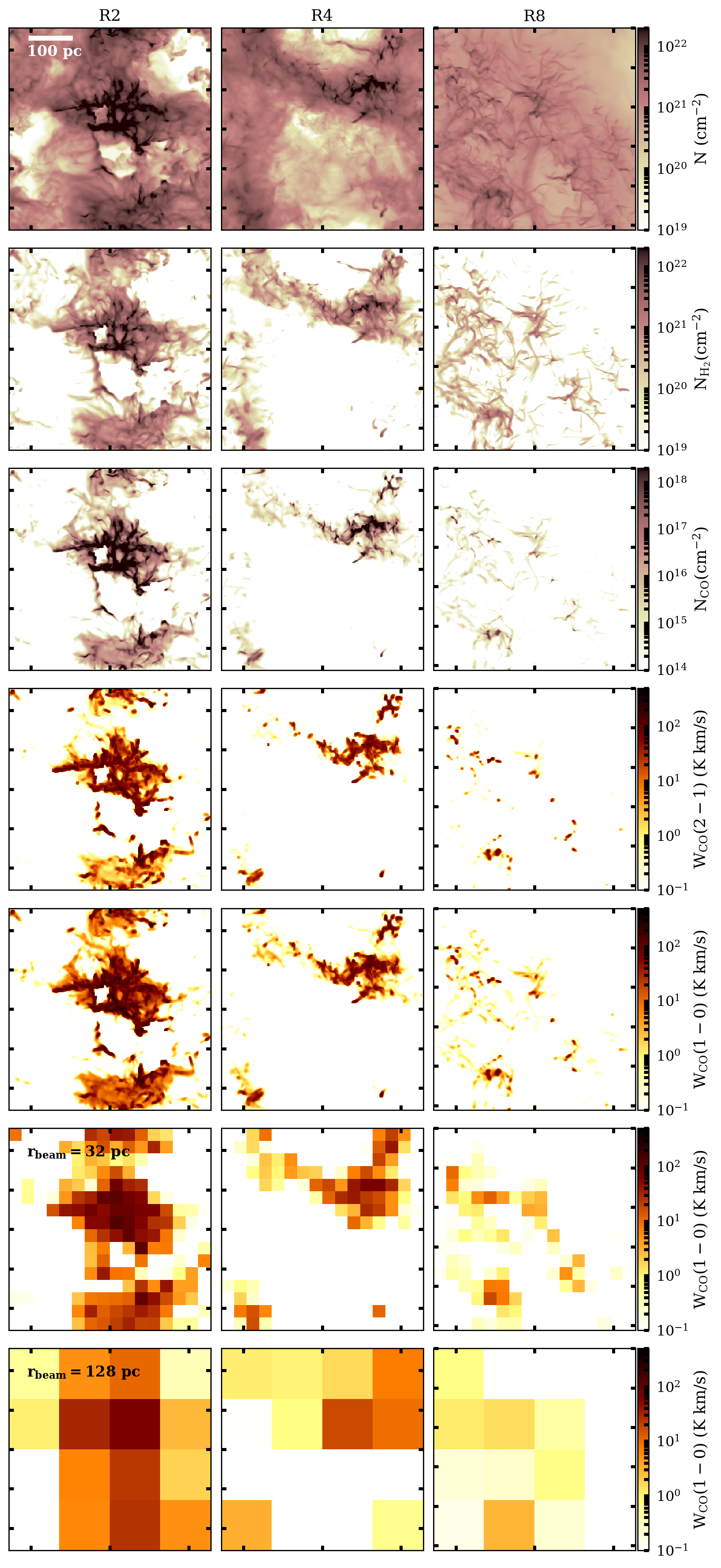
Results from representative snapshots taken from the R2, R4 and R8 fiducial physical models are shown in Figure 2. As the surface density decreases from the inner galaxy R2 model to solar neighborhood R8 model, the molecular clouds become smaller, less dense, and fainter in $\mathrm{CO}$ emission.

Comparing $N_{\mathrm{H_{2}}}$ and $N_{\mathrm{CO}}$, it is apparent that $\mathrm{CO}$ only traces the dense part of molecular clouds. The outskirts of diffuse molecular clouds are often $\mathrm{CO}$-dark. This is because $\mathrm{H_{2}}$ self-shielding of the destructive FUV radiation is very efficient, allowing $\mathrm{H_{2}}$ to form at lower column densities. The formation of $\mathrm{CO}$, on the other hand, requires sufficient dust shielding of the FUV radiation, which only occurs at higher column densities (Wolfire et al. 2010; Gong et al. 2017). As the surface density and density decrease, a larger fraction of $\mathrm{H_{2}}$ is in diffuse low density regions where $\mathrm{CO}$ is not present, leading to a higher fraction of $\mathrm{CO}$-dark $\mathrm{H_{2}}$ (see also Tables 4 and 5 and Section 4.4).

The maps of CO(2–1) and CO(1–0) line emission are very similar, with the (2–1) line slightly fainter and tracing slightly denser gas. While simulations are able to produce exquisite details of turbulent molecular clouds at $\sim\mathrm{pc}$ resolution, similar observational resolution is not available in extra-galactic observations. Even with the unprecedented angular resolution afforded by ALMA, as in the recent PHANGS survey, the physical resolution in galaxies beyond the Local Group is limited to $\gtrsim 20~{}\mathrm{pc}$, with $\sim 100~{}\mathrm{pc}$ more typical (Leroy et al. 2016; Sun et al. 2018). The last two rows of Figure 2 illustrate the effects of beam dilution. At 32 pc resolution, some substructures of GMCs can still be seen. At the coarser 128 pc resolution however, most pixels contain more than one cloud structure. The low surface density R8 models suffer the most from beam dilution. The small and faint clouds are smoothed out, and can fall under the observational detection limit in some cases.

Figure 3.— Mass-weighted histograms of $\log n$ (left), $\log N_{\mathrm{H_{2}}}$ (middle), and $W_{\mathrm{CO}}$-weighted histogram of $\log W_{\mathrm{CO}}$ ((1–0) line, right) in the snapshots shown in Figure 2 at the original resolution of 2 pc. All histograms are normalized to have the same area. The gray shaded region in the left panel is above the critical density for sink particle creation. As the total surface density increases from R8 to R4 and to R2 models, the distributions of $n$, $N_{\mathrm{H_{2}}}$, and $W_{\mathrm{CO}}$ also shift to higher values.

A more quantitative presentation of the gas properties for the fiducial models is shown in Figure 3. The peak of the mass-weighted density distribution increases by about two orders of magnitude from R8 to R2 models, and the peak of the $\mathrm{H_{2}}$ column density and CO brightness distributions also increases by about an order of magnitude. The higher density allows for more efficient formation of $\mathrm{H_{2}}$ and $\mathrm{CO}$ molecules and the higher surface density creates stronger shielding of the FUV radiation field. This allows the ISM near the mid-plane to transition from predominately atomic to predominately molecular from R8 to R2 models. We note that there is a sharp drop in the histogram of gas density $n$ at $\gtrsim 10^{3}~{}\mathrm{cm^{-3}}$, which is due to the numerical effect of sink particle creation. The peak of the density distribution, however, is well resolved at 2 pc resolution (GOK2018).

A summary of the important physical and observable variables across different models and snapshots at a synthetic beam sizes of 32 pc and 128 pc are listed in Tables 4 and 5 in the Appendix A. Many properties of molecular clouds vary significantly due to the changes in physical environments such as surface density, metallicity, FUV radiation field strength, and CRIR. The median values of $X_{\mathrm{CO},20}=0.6-3$ across different models show much less variation than the median values of both $N_{\mathrm{H_{2}}}$ and $W_{\mathrm{CO}}$, showing that $\mathrm{CO}$ emission traces $\mathrm{H_{2}}$ column density to some extent across all models. However, we also note that even in a given model, there is significant dispersion of $X_{\mathrm{CO}}$ across different regions and snapshots (as shown by the semi-quartile ranges in brackets), sometimes up to more than 50%. Taken together, this variability shows the need to calibrate $X_{\mathrm{CO}}$ to reduce the uncertainty in observations.

4.2. Comparison with Observations

Figure 4.— CO (2–1) line properties at GMC scales in PHANGS observations and our numerical simulations. The PHANGS observations, including the main sample and M33 in the Local Group, are taken from Sun et al. (2018), with a beam size of 120 pc. Only measurements in the disk regions and above the completeness limit for detection are included. The contours show the PHANGS data density levels including 10%, 50%, and 90% of the measurements. The yellow shaded areas roughly mark the regions below the observational detection limit. The simulations are taken from post-processing results with solar metallicity $Z=1$, and a beam-size of 128 pc. No detection limit is imposed in the simulations shown here, i.e, the simulated data points are assumed to have a perfect sensitivity. For the R2 and R4 models, post-processing results from different levels of FUV radiation and CRIR (-Z1, -Z1L10, -Z1CR10L10 models in Table 2) are all included, and their distributions are similar. For the R2 model, the larger box-size model (R2B2-Z1) is shown with empty triangles, and the higher numerical resolution model (R2N2-Z1) is shown with orange points, with the empty orange circles showing the corresponding lower resolution snapshot (in R2-Z1) at a similar simulation time. The range of physical parameters from the numerical simulations generally agree with the PHANGS observations, with some points below the observational detection limit. The estimation of the data density distribution is made using the fastKDE python package developed by O’Brien et al. (2014, 2016).

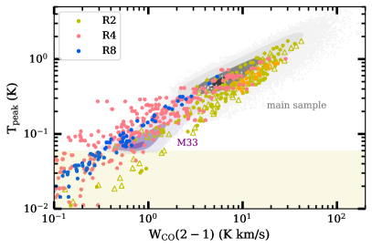
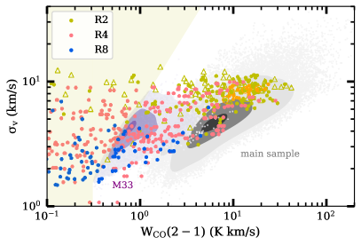
To validate that the molecular clouds in our simulations are realistic representations of observed clouds, we compare our simulation results to the cloud properties directly obtained from $\mathrm{CO}$ observations, such as $W_{\mathrm{CO}}$, $\sigma_{v}$, $T_{\mathrm{peak}}$ and $R_{21}$.

Figure 4 compares the molecular cloud properties traced by the CO(2–1) emission observed in the PHANGS galaxies (120 pc beam) with those in the synthetic observations from our simulations (128 pc beam). The simulations successfully reproduce both the correlations between and the range of the observed $W_{\mathrm{CO}}$, $T_{\mathrm{peak}}$ and $\sigma_{v}$. This confirms that the molecular clouds in our simulations are indeed realistic. Because we only simulate patches of galaxies, and do not account for the whole galactic environment, we cannot match the detailed statistical distribution of the observables in PHANGS. Our simulations suggest that many molecular clouds exist below the detection limit of PHANGS, especially in the lower surface density environments represented by the R4 and R8 models. The differences in the cloud properties observed in the nearby M33 and the main sample of PHANGS are at least partly due to the limited observational sensitivity. Even in our highest surface density model R2, many fainter clouds exist below the detection limit of the main sample in PHANGS, and the distribution smoothly extends to those observed in M33.

Figure 5.— Line ratio $R_{21}=W_{\mathrm{CO}}(2-1)/W_{\mathrm{CO}}(1-0)$ in comparison to observations, and for varying radiation and cosmic ray conditions. Left panel: Normalized histogram of $R_{21}$ for fiducial R4 model (R4-Z1) in comparison to the observations by Cormier et al. (2018) (C18). The observations of C18 have a spatial resolution of $\sim 1.5~{}\mathrm{kpc}$ and we show the simulated $R_{21}$ averaged over the whole 512 pc box, with the histogram showing the distribution from all temporal snapshots. The model reproduces the wide range of $R_{21}$ observed in C18. Middle and right panel: $R_{21}$ variations associated with variations in CRIR and FUV radiation. The middle panel shows the normalized histograms in models with CRIR 10 times lower (R4-Z1CR01) and higher (R4-Z1CR10) compared to the fiducial model R4-Z1. The right panel shows models with incident FUV radiation 10 times lower (R4-Z1L01) and higher (R4-Z1L10). Increasing either form of radiation moves the peak of the distribution to higher $R_{21}$.

Figure 5 shows the comparison of $R_{21}$ between our simulations and nearby spiral galaxies observed in the EMPIRE survey (Cormier et al. 2018). Most regions covered by the EMPIRE survey have a total gas surface density of $15-50~{}M_{\odot}\mathrm{pc^{-2}}$ and star formation rate of $0.01-0.1~{}M_{\odot}\mathrm{yr^{-1}kpc^{-2}}$ (Cormier et al. 2018; Jiménez-Donaire et al. 2019). This is closest to the R4 environment in our simulations, and thus we plot the R4-Z1 model for comparison. The left panel of Figure 5 shows that we successfully reproduce the observed distribution of $R_{21}$. This is a significant improvement over the one-zone model RADEX (van der Tak et al. 2007), which fails to reproduce the wide range of $R_{21}$ observed (see Figure 7 in Cormier et al. 2018). The middle and right panels of Figure 5 illustrate that increasing either the FUV radiation strength or CRIR tends to increase $R_{21}$. Qualitatively, this can be understood because both FUV radiation and CRs preferentially destroy CO in lower density gas, causing most of the $\mathrm{CO}$ emission to occur at higher densities, where $R_{21}$ is also higher on average. The mean values of $R_{21}$ in R4-Z1L01, R4-Z1 and R4-Z1L10, for which the background radiation field increases from 0.1 to 1 to 10 times the fiducial value, are 0.51, 0.65 and 0.82. A simple linear fit between $\log(J_{\mathrm{FUV}})$ and $R_{21}$ gives a slope of 0.152, close to the slope of 0.161 found in observations of M83 by Koda et al. (2020).

4.3. $X_{\mathrm{CO}}$ conversion factor

4.3.1 Dependence on Metallicity, FUV Radiation and Cosmic Rays

Figure 6.— The $X_{\mathrm{CO}}$ conversion factor for CO(1–0) (upper panels) and CO(2–1) (lower panels) lines. The x-axes correspond to parameter values encoded in model IDs, as given in Table 2; points in each group are slightly offset to left and right for clarity. Results for the R2, R4, and R8 models are shown in yellow, red, and blue colors, respectively. Points to the left of the main R2 simulations are from R2B2 (larger box size) and R2N2 (higher resolution) models, shown with dashed and dotted line styles. For all models, symbols and error bars show the median value $X_{\mathrm{CO}}$ and the semi-quartile range of $X_{\mathrm{CO}}$ in $\mathrm{CO}$-bright regions with a 32 pc (filled circle, thick error bar) and 128 pc (empty circle, thin error bar) beam (see also Tables 4 and 5). For each panel, the black dashed line shows a linear fit of $\log X_{\mathrm{CO}}$ (median values at 32 pc resolution, shown as the filled circles) as a function of the environmental parameters $\log Z$, $\log\xi_{0}$, $\log\chi_{0}$ and $\log f_{\mathrm{SFR}}$ (all models shown in each panel are included in the fits). Fitting with median values at 128 pc resolution gives very similar slopes. The fitted value of the slope and its standard deviation is written in the corresponding panel. Evidently, the main environmental drivers for the variation in $X_{\mathrm{CO}}$ are metallicity and the CRIR.

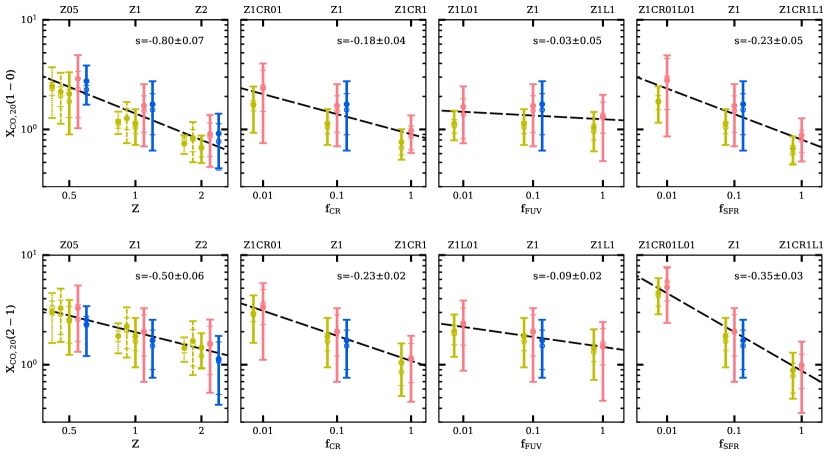
Figure 6 summarizes results of $X_{\mathrm{CO}}$ from all of our models for both the $J=1-0$ (top) $J=2-1$ (bottom) lines, separately showing variations due to metallicity, FUV radiation, and CRIR when the parameters $Z$, $f_{\mathrm{CR}}$, $f_{\mathrm{FUV}}$ are independently varied, and when the last two are varied together as $f_{\mathrm{SFR}}$. The R2B2 (larger box size) and R2N2 (higher resolution) models have very similar $X_{\mathrm{CO}}$ to the fiducial R2 model. This confirms that $X_{\mathrm{CO}}$ is converged at the current box size and 2 pc resolution, as previously found in GOK2018.

Figure 6 also shows results of fitting the variation of $X_{\mathrm{CO}}$ with varying metallicity ($Z$), CRIR ($\xi_{0}$), and background FUV strength ($\chi_{0}$). As expected (see Section 2), $X_{\mathrm{CO}}$ decreases with increasing $Z$. It is interesting that the measured scalings $X_{\mathrm{CO}}(1-0)\propto Z^{-0.8}$ and $X_{\mathrm{CO}}(2-1)\propto Z^{-0.5}$ are similar to the relation $X_{\mathrm{CO}}\propto Z^{-1/2}$ predicted based on a highly simplified model in Equation 9, under the assumption $n_{\mathrm{CO}}\propto Z$ in CO-emitting regions. The physical reason for the increase of $X_{\mathrm{CO}}$ at lower $Z$ is the decreased excitation temperature due to lower optical depth of CO lines (see also Figure 8 and related text), although the lines are still optically thick. Compared to the (1–0) line, the (2–1) line traces denser gas where the CO abundance is less sensitive to the change in dust shielding (as the shielding is already above the critical values required for CO formation), and thus shows a weaker dependence on $Z$.

Also consistent with general expectations, considering the decrease of $X_{\mathrm{CO}}$ at higher $T_{\mathrm{gas}}$ (see Equation 3 and Equation 4) and the increase of $T_{\mathrm{gas}}$ at higher CRIR in shielded regions, $X_{\mathrm{CO}}$ decreases roughly $\propto\xi_{0}^{-0.2}$. There is also very weak dependence on the FUV radiation field, roughly $X_{\mathrm{CO}}(1-0)\propto\chi_{0}^{-0.03}$ or $X_{\mathrm{CO}}(2-1)\propto\chi_{0}^{-0.09}$. This insensitivity is reasonable, given that FUV mainly affects the gas volume and mass where CO and $\mathrm{H_{2}}$ can form (limited by photodissociation), rather than the conditions in shielded regions.

Since $Z$ is often readily available in observations, the fits shown in Figure 6 (see also 1a and 1b in Table 3) can be used to calibrate $X_{\mathrm{CO}}$ in different galactic environments. While the dependence of $X_{\mathrm{CO}}$ on the CRIR is also quite clear from our simulations, the value $\xi_{0}$ is not easily accessible observationally. Since the physical dependence on $\xi_{0}$ is expected to be mainly through the gas temperature, which affects excitation, other avenues to controlling for this effect are available. We discuss this further below.

Figure 7.— Gas temperature $T_{\mathrm{gas}}$ (orange) and CO(1–0) line excitation temperature $T_{\mathrm{exc}}$ (black) from the snapshots shown in Figure 2. The binned average values with standard deviations are shown together with the background scatter of individual pointings. The excitation temperature approaches the gas temperature at densities $n\gtrsim 500~{}\mathrm{cm^{-3}}$. The $T_{\mathrm{exc}}$ – $n$ relation is important for $X_{\mathrm{CO}}$ (Equation 2 and 3).

Figure 8.— Dependence on density of $T_{\mathrm{gas}}$ and $T_{\mathrm{exc}}$ as in Figure 7, but for just model R4 at varying CRIR, FUV intensity, and metallicity. Compared to the middle panel of Figure 7, here we show: (top row) CRIR 10 times lower (R4-Z1CR01) or higher (R4-Z1CR10); (middle row) incident FUV radiation 10 times lower (R4-Z1L01) or higher (R4-Z1L10); (bottom row) metallicity 2 times lower (R4-Z05) and higher (R4-Z2).

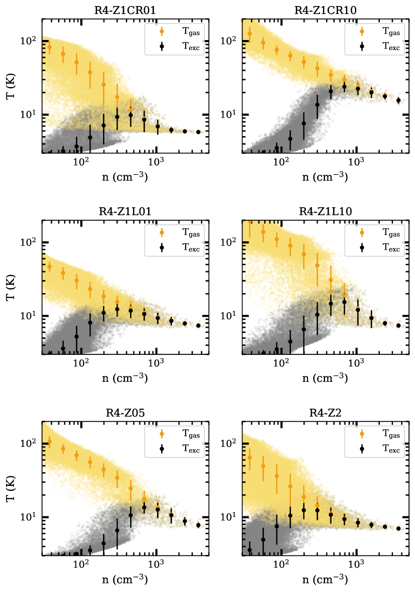
Motivated by the theoretical expectations (see Equations 3, 4, and 7), we further examine the relation between $T_{\mathrm{exc}}$ and $n$ in Figures 7 and 8. At low density, there is a large difference between $T_{\mathrm{exc}}$ and $T_{\mathrm{gas}}$. As the density increases, $T_{\mathrm{exc}}$ increases both due to the higher collisional rates and the increased optical depth. At the same time, $T_{\mathrm{gas}}$ decreases due to decreased heating from the shielding of the FUV radiation (and CRs), and increased cooling at higher densities. As pointed out by Gong et al. (2017), because FUV radiation dissociates $\mathrm{CO}$, the $\mathrm{CO}$-rich regions are generally shielded by high columns of dust, and CR ionization dominates heating of the gas. At high enough density (cf. Equations 4 and 10), $T_{\mathrm{exc}}$ reaches LTE with $T_{\mathrm{gas}}$. In shielded gas, $T_{\mathrm{gas}}$ is mostly set by the CRIR, and decreases slightly at high densities due to the decrease in low-energy cosmic rays penetrating to high columns (following our adopted relation in Equation 12). Although $\xi_{0}$ is higher in R2 models, there is also more shielding due to the higher surface density (see also Table 2). As a result, the CRIR and temperature in the $\mathrm{CO}$ dominated gas are similar across the fiducial R2, R4 and R8 models. At lower densities where $T_{\mathrm{exc}}<T_{\mathrm{gas}}$, the $T_{\mathrm{exc}}$ values in R2 models are slightly higher due to the higher optical depth. This leads to the slightly lower $X_{\mathrm{CO}}$ in the fiducial R2 models (Equation 3).

Figure 8 further examines the $T_{\mathrm{exc}}$ – $n$ relation in models with varying CRIR, FUV radiation and metallicity. Increasing the CRIR (top row) leads to higher temperature in the dense, shielded regions, resulting in higher $T_{\mathrm{exc}}$; this is the reason for the decrease of $X_{\mathrm{CO}}$ at higher $f_{\mathrm{CR}}$ seen in Figure 6. An increase in the FUV radiation (second row) also increases the gas temperature, but only in the low density and minimally shielded gas. At the same time, photodissociation of $\mathrm{CO}$ decreases the optical depth. These two effects tend to cancel each other, and as a result, the $X_{\mathrm{CO}}$ is relatively insensitive to the FUV radiation (as seen in the weak dependence on $f_{\mathrm{FUV}}$ in Figure 6). Increasing metallicity (third row) leads to more shielding and more efficient $\mathrm{CO}$ formation. At low (high) $Z$, line saturation – with $T_{\mathrm{exc}}$ approaching $T_{\mathrm{gas}}$ – occurs at higher (lower) densities. Overall, an increase in $Z$ results in higher optical depth, higher $T_{\mathrm{exc}}$, and lower $X_{\mathrm{CO}}$.

Figure 9.— Summary of results for $X_{\mathrm{CO}}(1-0)$ versus $Z$. The yellow, red and blue error bars and the black dashed line show the results from our fiducial R2, R4 and R8 models as in the top left panel of Figure 6, with slight horizontal offsets to avoid overlaps. We compare to other theoretical predictions (green lines) and observations (gray lines and symbols), as follows. Wolfire et al. (2010): PDR models. Narayanan et al. (2012) and Feldmann et al. (2012): Galaxy simulations with sub-grid models for molecular clouds. Accurso et al. (2017): numerical models of spherically symmetric star forming regions. Leroy et al. (2011): observations of local group galaxies, averaged over large areas comparable to the size of the galaxy; $\mathrm{H_{2}}$ mass from dust. Sandstrom et al. (2013): nearby spiral and dwarf galaxies, averaged over kilo-parsec scale; $\mathrm{H_{2}}$ mass from dust. Our results and fit $X_{\mathrm{CO}}(1-0)\propto Z^{-0.8}$ in the range of $Z=0.5-2$ are consistent with other theoretical predictions and observations.

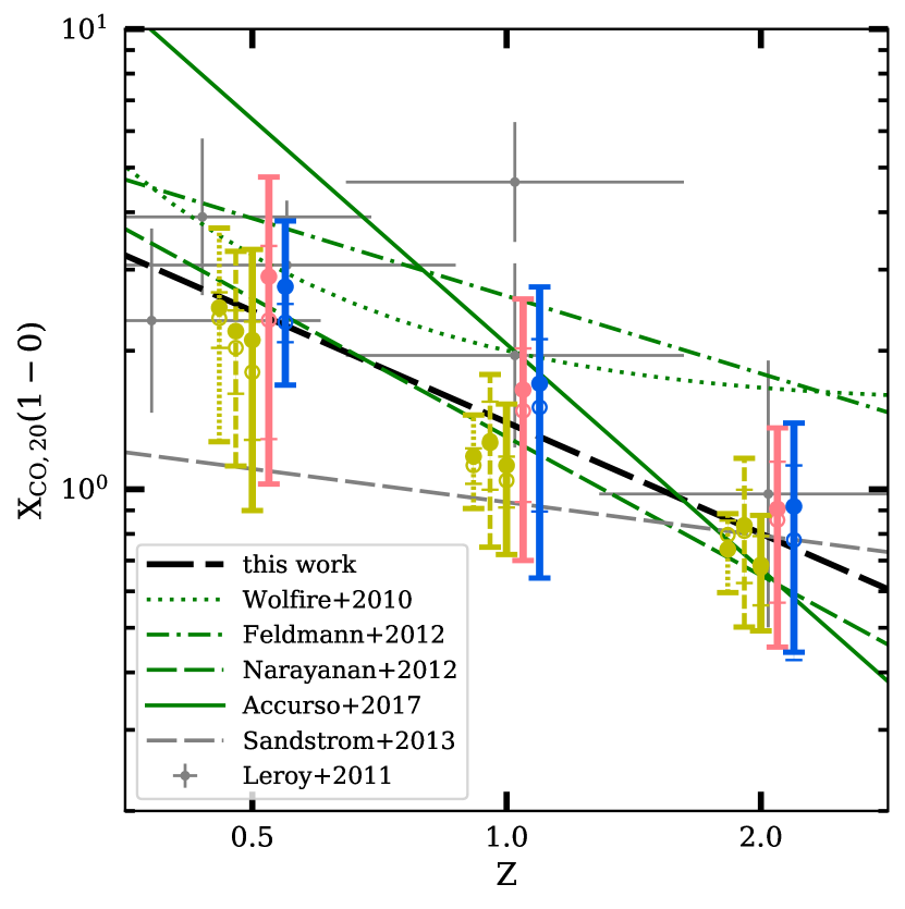
Of the “environmental” factors affecting $X_{\mathrm{CO}}$, the dependence on $Z$ has been the most extensively studied in theory and observations. We show a comparison between our results and recent literature in Figure 9. Among the theoretical studies shown, our work is the only one that has resolved clouds forming (and dispersing) in time-dependent simulations of the multiphase ISM with self-consistent star formation and feedback. The slope of $-0.8$ found by us for $X_{\mathrm{CO}}(1-0)$ lies in between other theoretical predictions. Our values of $X_{\mathrm{CO}}$ are also consistent with observations of the Milky Way and nearby galaxies. We note that our results are only valid between $Z=0.5-2$. The MHD simulations are run with $Z=1$, and a large departure from $Z=1$ can change the dynamical structure of the clouds where molecules form by changing the efficiency of heating and cooling. Furthermore, at lower metallicities, decreased shielding causes $\mathrm{CO}$ to form at higher densities, which would require higher numerical resolution. We have experimented with setting $Z=0.1$, and found that current resolution of 1 – 2 pc is inadequate in order to resolve $X_{\mathrm{CO}}$.

4.3.2 Dependence on Physical Properties of the Gas

While in Section 4.3.1 we investigate the variation of average $X_{\mathrm{CO}}$ on large scales associated with key environmental factors, in this section we consider the variation of $X_{\mathrm{CO}}$ on small scales due to the structure and spatially-varying conditions within molecular clouds.

Figure 10.— $N_{\mathrm{H_{2}}}$ versus $W_{\mathrm{CO}}(1-0)$ for the R2-Z1 (yellow), R4-Z1 (red) and R8-Z1 (blue) snapshots shown in Figure 2 at the native simulation resolution of 2 pc. The binned mean values and standard deviations are plotted over the background of scattered individual points. The dashed lines show the average $X_{\mathrm{CO}}$ in the CO-bright ($W_{\mathrm{CO}}>0.75~{}\mathrm{K\cdot km/s}$) regions for each model.

Figure 11.— Correlation between $X_{\mathrm{CO}}(1-0)$ and physical properties of the gas for the R2-Z1 (yellow), R4-Z1 (red) and R8-Z1 (blue) snapshots shown in Figure 2. The parameters $\langle n\rangle_{M_{CO}}$, $\langle T_{\mathrm{exc}}\rangle_{M_{CO}}$, $\langle|\mathrm{d}v/\mathrm{d}r|\rangle_{M_{CO}}$, and $\langle\sigma_{v}\rangle_{M_{CO}}$ are the gas density, excitation temperature of the $J=1-0$ transition, the velocity gradient, and velocity dispersion along the line of sight, weighted by the $\mathrm{CO}$ mass. Each point represents a pixel at the native simulation resolution of 2 pc. The binned median values and semi-quartile range are plotted over the background of scatter points for the left two panels (medians are not shown in the right two panels, where no significant correlation is found). Only pixels with $W_{\mathrm{CO}}>2~{}\mathrm{K\cdot km/s}$ are shown.

Figure 12.— Correlation between $R_{21}$ and physical properties of the gas, similar to Figure 11.

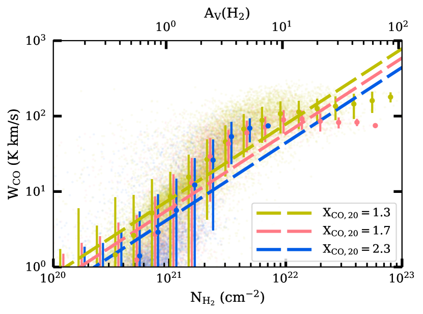
First, it is evident from the $W_{\mathrm{CO}}$ – $N_{\mathrm{H_{2}}}$ relation illustrated in Figure 10 that $X_{\mathrm{CO}}$ systematically varies with surface density at small scales within molecular clouds. On the one hand, at low $N_{\mathrm{H_{2}}}$ the $\mathrm{CO}$ abundance is low due to photodissociation at low $A_{V}$, whereas $\mathrm{H_{2}}$ is non-negligible, being self-shielded. On the other hand, at high $N_{\mathrm{H_{2}}}\gtrsim 5\times 10^{21}~{}\mathrm{cm^{-2}}$ the relation flattens as $W_{\mathrm{CO}}$ saturates due to the high optical depth. As a result, the resolved $W_{\mathrm{CO}}$ vs. $N_{\mathrm{H_{2}}}$ relations are steeper than the large-scale averages (shown as dashed lines) in the range $N_{\mathrm{H_{2}}}\sim 0.7-5\times 10^{21}~{}\mathrm{cm^{-2}}$. To obtain the correct $N_{\mathrm{H_{2}}}$, an $X_{\mathrm{CO}}$ higher than the large-scale average would be required at $N_{\mathrm{H_{2}}}\lesssim 2\times 10^{21}~{}\mathrm{cm^{-2}}$ ($A_{V}\lesssim 2$), whereas an $X_{\mathrm{CO}}$ lower than the large-scale average would be required at $N_{\mathrm{H_{2}}}\gtrsim 2\times 10^{21}~{}\mathrm{cm^{-2}}$ ($A_{V}\gtrsim 2$). Similar trends are also found in high resolution observations of local molecular clouds (Pineda et al. 2008; Lee et al. 2018), simulations of individual molecular clouds (Shetty et al. 2011a, b; Szűcs et al. 2016) and zoom-in simulations (Seifried et al. 2020).

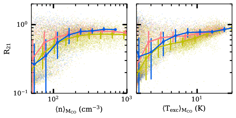
Inspired by Equations 2 – 10, we investigate the correlation between $X_{\mathrm{CO}}$ and physical properties of the gas on small scales in Figure 11. The left panel directly shows that $X_{\mathrm{CO}}$ first decreases and then increases with density, consistent with the theoretical expectations from Equations 9 and 10. The $X_{\mathrm{CO}}$ – $T_{\mathrm{exc}}$ relation shown in the second panel can be explained by reference to Equation 8 and Equation 9. If $f_{\mathrm{CO}}$ and $|\mathrm{d}v/\mathrm{d}r|$ are constant or have no systematic variation in $\mathrm{CO}$-bright regions, then $T_{\mathrm{exc}}\propto n$ and $X_{\mathrm{CO}}\propto{T_{\mathrm{exc}}}^{-1/2}$. The right two panels of Figure 11 show that $X_{\mathrm{CO}}$ is uncorrelated with the local velocity gradient $|\mathrm{d}v/\mathrm{d}r|$ and the large scale velocity dispersion along the line of sight.

Figure 12 examines the relation between $R_{21}$ and gas properties. $R_{21}$ is high at higher $n$ and $T_{\mathrm{exc}}$, and has a large scatter at lower $n$ and $T_{\mathrm{exc}}$. This is consistent with the observations by Koda et al. (2020), who found that $R_{21}$ has a large spread in regions with low $W_{\mathrm{CO}}$, and $R_{21}$ is high in regions with high $W_{\mathrm{CO}}$. Because $R_{21}$ correlates with $n$ and $T_{\mathrm{exc}}$, it also correlates with $X_{\mathrm{CO}}$, and we use this to calibrate $X_{\mathrm{CO}}$ in Section 4.3.3.

4.3.3 Calibrating $X_{\mathrm{CO}}$ Using Observable Quantities

Table 3Fitting Results: $X_{\mathrm{CO}}$ as a function of observables

Number	Transition	Parameters	Fitting Result
1a	1-0	$Z$	$X_{\mathrm{CO,20}}=1.4Z^{-0.80}$
1b	2-1	$Z$	$X_{\mathrm{CO,20}}=2.0Z^{-0.50}$
2a	1-0	$R_{21},Z,r_{\mathrm{beam}}$	$X_{\mathrm{CO,20}}=0.93(R_{21}/0.6)^{-0.87}Z^{-0.80}(\mathrm{min}\{r_{\mathrm{beam}},100\})^{0.081}$
2b	2-1	$R_{21},Z,r_{\mathrm{beam}}$	$X_{\mathrm{CO,20}}=1.5(R_{21}/0.6)^{-1.69}Z^{-0.50}(\mathrm{min}\{r_{\mathrm{beam}},100\})^{0.063}$
3a	1-0	$T_{\mathrm{peak}},Z,r_{\mathrm{beam}}$	$X_{\mathrm{CO,20}}=1.8T_{\mathrm{peak}}^{-0.64+0.24\log r_{\mathrm{beam}}}Z^{-0.80}r_{\mathrm{beam}}^{-0.083}$
3b	2-1	$T_{\mathrm{peak}},Z,r_{\mathrm{beam}}$	$X_{\mathrm{CO,20}}=2.7T_{\mathrm{peak}}^{-1.07+0.37\log r_{\mathrm{beam}}}Z^{-0.50}r_{\mathrm{beam}}^{-0.13}$
4a	1-0	$W_{\mathrm{CO}},Z,r_{\mathrm{beam}}$	$X_{\mathrm{CO,20}}=6.1W_{\mathrm{CO}}^{-0.54+0.19\log r_{\mathrm{beam}}}Z^{-0.80}r_{\mathrm{beam}}^{-0.25}$
4b	2-1	$W_{\mathrm{CO}},Z,r_{\mathrm{beam}}$	$X_{\mathrm{CO,20}}=21.1W_{\mathrm{CO}}^{-0.97+0.34\log r_{\mathrm{beam}}}Z^{-0.50}r_{\mathrm{beam}}^{-0.41}$

Figure 13.— Comparison of the $X_{\mathrm{CO}}$ fits to true values, binned by $W_{\mathrm{CO}}$. The symbols and error bars are the median value and semi-quartile range in each $W_{\mathrm{CO}}$ bin. The upper rows are for the CO(1–0) line and the lower rows the CO(2–1) line. The left, middle, and right columns are for synthetic observation with beam-sizes $r_{\mathrm{beam}}=2$, $32$, and $128~{}\mathrm{pc}$. The black lines use the fit given in expressions 1a/b of Table 3 that depends only on $Z$. In this case, $X_{\mathrm{CO}}$ is under-estimated in $\mathrm{CO}$-faint regions for small beams. The purple lines use the fit $X_{\mathrm{CO}}(R_{21},Z,r_{\mathrm{beam}})$ that takes into account line ratios (expressions 2a/b in Table 3), which performs quite well overall. The orange and green lines represent the fits $X_{\mathrm{CO}}(T_{\mathrm{peak}},Z,r_{\mathrm{beam}})$ and $X_{\mathrm{CO}}(W_{\mathrm{CO}},Z,r_{\mathrm{beam}})$ (expressions 3a/b and 4a/b in Table 3), which perform well in regions with low and moderate $W_{\mathrm{CO}}$, but under-estimate $X_{\mathrm{CO}}$ in the most CO-bright regions ($W_{\mathrm{CO}}\gtrsim 20~{}\mathrm{K\cdot km/s}$).

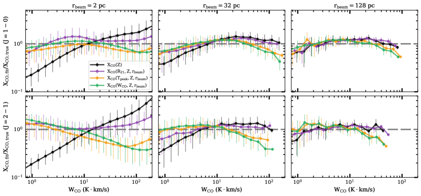
As pointed out in Section 4.3.2, there are significant systematic variations in $X_{\mathrm{CO}}$ on small scales, correlated with the gas density and excitation temperature. While these correlations reflect inherent dependencies on physical conditions, neither the density nor the excitation temperature is readily available from observations. As a proxy, we identify direct observable quantities that reflect physical conditions in a similar way, and use them to calibrate $X_{\mathrm{CO}}$ on small scales.

We consider the following observables: the metallicity $Z$, the line ratio $R_{21}$, the peak antenna temperature $T_{\mathrm{peak}}$, the integrated line intensity $W_{\mathrm{CO}}$, and the line width $\sigma_{v}$. We select the models R[2,4,8]-Z[05,1,2] and R2B2-Z[05,1,2]. As discussed in subsection 3.2 (see also Table 2), these models have FUV radiation field that matches the observed SFRs, which in R2 and R4 models requires a reduction relative to the MHD model itself (the CRIR is scaled relative to the FUV). The range of metallicity extends a factor of 2 above and below the solar neighborhood.

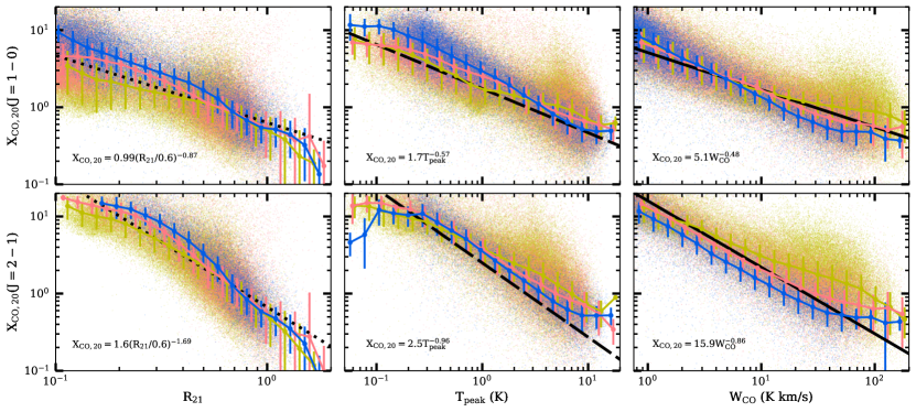
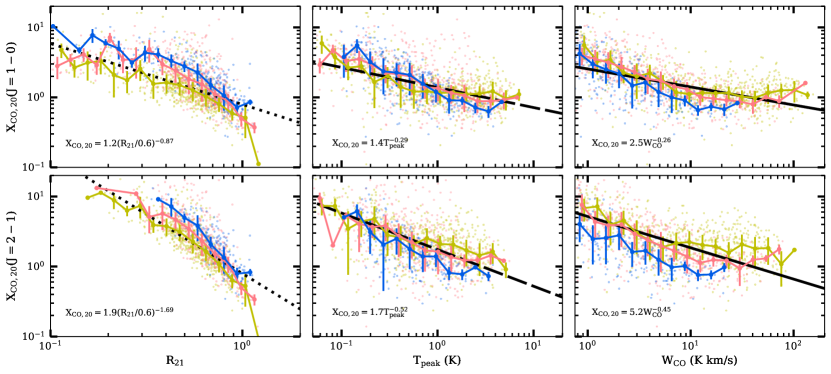
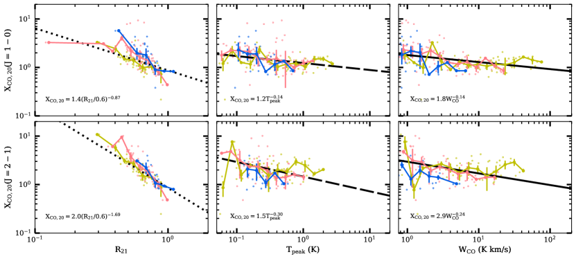
Figures 15, 16 and 17 (see Appendix A) show the values of $X_{\mathrm{CO}}(1-0)$ and $X_{\mathrm{CO}}(2-1)$ for all $Z=1$ models as functions of observables $R_{21}$, $T_{\mathrm{peak}}$, and $W_{\mathrm{CO}}$, for beam size $2$ pc, $32$ pc, and $128$ pc, respectively. For each observable and the range of beam sizes, we perform simple log-linear fits using the least-squares method between the observable and $X_{\mathrm{CO}}$, combining data from R2, R4, and R8 models. Each data point in the fitting represents a pixel in the synthetic observation, and the fits are weighted by the area of the pixel. We limit the fitting to $\mathrm{CO}$-bright regions of $W_{\mathrm{CO}}>0.75~{}\mathrm{K\cdot km/s}$. The $X_{\mathrm{CO}}$-$T_{\mathrm{peak}}$ and $X_{\mathrm{CO}}$-$W_{\mathrm{CO}}$ relations are shallower at larger beam sizes due to beam-dilution. Therefore, we include an additional term $\log r_{\mathrm{beam}}$ in the power-law exponents of $T_{\mathrm{peak}}$ and $W_{\mathrm{CO}}$ to capture this effect. Due to beam-averaging, $X_{\mathrm{CO}}$ is roughly constant when beam sizes are large, and we therefore limit the fitting to $r_{\mathrm{beam}}\leq 128~{}\mathrm{pc}$. We also tested $\sigma_{v}$, but found that it does not show any significant correlation with $X_{\mathrm{CO}}$, as expected from Section 4.3.2; we therefore did not include it in the final results. In addition, we experimented with fitting $\sigma_{v}$ together with other observables, and found no significant improvement in the fit using the Bayesian information criteria. We fix the slopes for the $Z$ dependence ($X_{\mathrm{CO}}(1-0)\propto Z^{-0.8}$ and $X_{\mathrm{CO}}(2-1)\propto Z^{-0.5}$), which were obtained from fitting of median $X_{\mathrm{CO}}$ values in models with different metallicity (see Section 4.3.1 and Figure 6). We also tried fitting the $X_{\mathrm{CO}}$ – $Z$ relation using all pixels at the same time, as we do for other variables, and obtained very similar slopes for $Z$.

As can be seen from Figures 15, 16 and 17, the values of $X_{\mathrm{CO}}$ have large intrinsic scatter at a given $R_{21}$, $T_{\mathrm{peak}}$, or $W_{\mathrm{CO}}$. This implies that other hidden variables that are not directly observable, such as the detailed gas density, temperature, and velocity structure along the line of sight, also influence $X_{\mathrm{CO}}$. Although the relations between $X_{\mathrm{CO}}$ and the various observables are not true power-laws, we find that the power-law fit we adopted already captures most of the systematic variations in the data. We find that the (absolute) difference between the fitted $X_{\mathrm{CO}}$ and the median values of $X_{\mathrm{CO}}$ in each bin is much smaller than the standard deviation of $X_{\mathrm{CO}}$ in each bin, except for the most CO-bright regions with $W_{\mathrm{CO}}\gtrsim 20~{}\mathrm{K\cdot km/s}$. Even for $20~{}\mathrm{K\cdot km/s}\lesssim W_{\mathrm{CO}}\lesssim 200~{}\mathrm{K\cdot km/s}$, the systematic errors from the power-law fit are still smaller than or comparable to the intrinsic scatter in $X_{\mathrm{CO}}$ (see also Figure 13).

Table 3 summarizes the results of our fitting. In expressions 1a/b, we provide our results for the relation with metallicity only from Figure 6. Relations 2a/b, 3a/b, and 4a/b give our calibrations for $X_{\mathrm{CO}}$ when the independent variable is $R_{21}$, $T_{\mathrm{peak}}$, or $W_{\mathrm{CO}}$, respectively. We note that $W_{\mathrm{CO}}$, $T_{\mathrm{peak}}$ and $R_{21}$ are highly correlated, and therefore our fitted relationships should be considered as set of alternative (rather than “multiplicative”) calibrations for $X_{\mathrm{CO}}$.

The fits for $X_{\mathrm{CO}}$ as functions of $R_{21}$, $T_{\mathrm{peak}}$, and $W_{\mathrm{CO}}$ are included as dotted, dashed, and solid lines in Figures 15, 16 and 17. $R_{21}$, $T_{\mathrm{peak}}$ and $W_{\mathrm{CO}}$ all increase with increasing gas density and excitation temperature, and thus negatively correlate with $X_{\mathrm{CO}}$. At very high density $n\gtrsim 300~{}\mathrm{cm^{-3}}$ where the optical depth for $\mathrm{CO}$ is very large, the turn-over of $X_{\mathrm{CO}}$ in the left panel of Figure 11 is reflected in the flattening of the binned $X_{\mathrm{CO}}$ values near $W_{\mathrm{CO}}\approx 100~{}\mathrm{K\cdot km/s}$ and $T_{\mathrm{peak}}\approx 10~{}\mathrm{K}$. $W_{\mathrm{CO}}\approx 100~{}\mathrm{K\cdot km/s}$ also corresponds to the saturation level at $N_{\mathrm{H_{2}}}\gtrsim 5\times 10^{21}~{}\mathrm{cm^{-2}}$ in Figure 10. For the current physical conditions and resolution in our simulations, most of the $\mathrm{CO}$ emission comes from lower density regions where the trend in Equation 9 is expected. $X_{\mathrm{CO}}$ decreases with increasing $W_{\mathrm{CO}}$ and $T_{\mathrm{peak}}$ for the majority of the data points at high resolution. Therefore, we simply use a single power-law fit. We do note, however, that our fits should not be applied to molecular cloud regions with $W_{\mathrm{CO}}\gtrsim 200~{}\mathrm{K\cdot km/s}$ where the lines are saturated.

Comparing Figures 15, 16 and 17, it is apparent that the scaling of $X_{\mathrm{CO}}$ with $T_{\mathrm{peak}}$ or $W_{\mathrm{CO}}$ is shallower at a larger $r_{\mathrm{beam}}$ due to beam-dilution. The slopes for the $X_{\mathrm{CO}}$ fits are steeper for the (2–1) line, which traces regions with denser gas and higher excitation temperature than the (1–0) line.

A comparison between all the $X_{\mathrm{CO}}$ fits and the original measurements, binned by $W_{\mathrm{CO}}$, is shown in Figure 13. We present results separately for $2$ pc, $32$ pc, and $128$ pc beams. For smaller ($2$ pc or $32$ pc) beams, the simple $X_{\mathrm{CO}}$ – $Z$ relation is systematically biased: at low $W_{\mathrm{CO}}\lesssim 10~{}\mathrm{K\cdot km/s}$, the relation 1a/b underestimates the true $X_{\mathrm{CO}}$, while at high $W_{\mathrm{CO}}\gtrsim 10~{}\mathrm{K\cdot km/s}$, the relation 1a/b slightly ($32$ pc) or significantly ($2$ pc) overestimates the true $X_{\mathrm{CO}}$. This can be problematic when calculating masses of molecular clouds with a large range of local physical conditions and brightness. However, any of the three observables tested here can help to correct this systematic bias. $R_{21}$ performs the best across a large range of $W_{\mathrm{CO}}$, and the correlation is insensitive to the beam-size. $W_{\mathrm{CO}}$ and $T_{\mathrm{peak}}$ perform well in regions with low and moderate $W_{\mathrm{CO}}$, but under-estimate $X_{\mathrm{CO}}$ when $W_{\mathrm{CO}}\gtrsim 20~{}\mathrm{K\cdot km/s}$, with $T_{\mathrm{peak}}$ giving slightly better results.

At $r_{\mathrm{beam}}\gtrsim 100~{}\mathrm{pc}$, there is already significant averaging over varying density, temperature, etc. within each beam, and we find that $X_{\mathrm{CO}}$ is consistent with having no correlation with $T_{\mathrm{peak}}$ or $W_{\mathrm{CO}}$. The $X_{\mathrm{CO}}$ dependencies on $Z$ and $R_{21}$, however, reflect the conditions for CO formation and excitation on all scales, and therefore do not suffer from beam dilution. In particular the $X_{\mathrm{CO}}$ relation with $R_{21}$ (2a/b in Table 3) only has a very weak dependence on $r_{\mathrm{beam}}$ for the overall scaling at small beam sizes, and the dependence vanishes as beam sizes increase to $\gtrsim 100~{}\mathrm{pc}$. Therefore, for large beams, we recommend using the simple $X_{\mathrm{CO}}$ – $Z$ relation (1a/b in Table 3) if only a single line is available, or preferably the $X_{\mathrm{CO}}$ – $R_{21}$ relation (2a/b) since this helps to capture the increase in excitation (and CO emission) in regions of higher mean density or where gas temperatures are enhanced by stronger heating.

4.4. $\mathrm{CO}$-dark $\mathrm{H_{2}}$

Figure 14.— Fraction of CO-dark $\mathrm{H_{2}}$ as a function of the detection limit in the fiducial models (see legend), for both the (1–0) (top panel) and the (2–1) (bottom panel) lines. The different line styles show results from different beam-sizes $r_{\mathrm{beam}}=2~{}\mathrm{pc}$ (solid lines), $32~{}\mathrm{pc}$ (dashed lines) and $128~{}\mathrm{pc}$ (dotted lines). The vertical gray line shows the default detection limit in our studies.

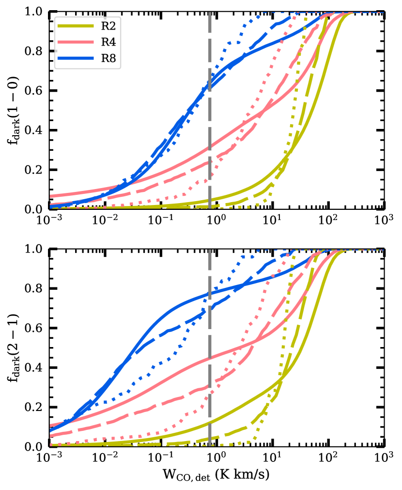
Finally, we investigate $f_{\mathrm{dark}}$, the CO-dark $\mathrm{H_{2}}$ fraction (defined in Equation 11). Figure 14 shows that in addition to the detection limit, $f_{\mathrm{dark}}$ also depends on the gas surface density, and to a lesser extent, the beam-size. In the lower surface density R8 models, the clouds are fainter and smaller, and thus fall more easily under the detection limit compared to the brighter clouds in R4 and R2 models. At the fiducial detection limit of $0.75~{}\mathrm{K\cdot km/s}$, almost all the $\mathrm{H_{2}}$ in the R2 model would be detected via $\mathrm{CO}$, while more than half of the $\mathrm{H_{2}}$ mass remains CO-dark in the R8 model (see also Tables 4 and 5).

Pety et al. (2013) analysed CO (1-0) line emission in M51 using different observational data sets, and found that about $50\pm 10\%$ of the emission is undetected at a resolution of 40 pc and sensitivity of $0.4~{}\mathrm{K\cdot km/s}$ ($1\sigma$). The average surface density is about $30M_{\odot}\,{\rm pc}^{-2}$ in the regions they observed, similar to that in our R4 models. We find that $f_{\mathrm{dark}}=30\%$ for the R4 models with $r_{\mathrm{beam}}=32~{}\mathrm{pc}$ and $3\sigma$ detection limit of $1.2~{}\mathrm{K\cdot km/s}$, which can already account for most of the missing emission in Pety et al. (2013).

We also note from Table 4 and Table 5 that all models have a decrease in the fraction of CO-dark gas at higher $Z$. However, especially for R2 and R4 models, $1-f_{\mathrm{dark}}$ varies little with $Z$. Since the majority of $\mathrm{H_{2}}$ is in CO-bright regions (for the range $Z=0.5-2$). This implies that in large-beam observations, the translation of CO luminosity to $\mathrm{H_{2}}$ mass will depend on $Z$ mainly through the opacity of optically-thick lines (which affect the excitation temperature), as previously discussed (see Figure 8 and related text).

5. Conclusions

In this paper, we use numerical simulations of the multiphase, star-forming ISM in galactic disks to study the properties of the molecular component and the $X_{\mathrm{CO}}$ conversion factor that is used to obtain $N_{\mathrm{H_{2}}}$ from $W_{\mathrm{CO}}$. We extend the previous work of GOK2018 based on simulations with solar neighborhood conditions to a wide range of galactic environments. We post-process 3D MHD simulations with chemistry and radiation transfer solvers to produce synthetic maps of CO(1–0) and CO(2–1) emission lines. We confirm numerical convergence of our results for $X_{\mathrm{CO}}$ by varying the spatial resolution and box size.

Our study investigates the dependencies on $X_{\mathrm{CO}}$ on large-scale environmental parameters (metallicity, FUV radiation intensity, CRIR), local physical properties of the gas (density, excitation temperature), and observables (CO brightness, peak temperature of the line, line ratio), as well as averaging scale (beam size). Our main findings are as follows:

1. We successfully reproduce the relations between the $\mathrm{CO}$ peak brightness temperature $T_{\mathrm{peak}}$, the line width $\sigma_{v}$, and the brightness $W_{\mathrm{CO}}$ in the PHANGS survey of nearby galaxies (Figure 4), as well as the distribution of $R_{21}$, the CO (2–1) to (1–0) line ratio, in the EMPIRE survey (Figure 5). We also found a similar relation between $R_{21}$ and the FUV radiation field strength to that observed in M83 (Koda et al. 2020). This confirms that the molecular medium in our simulations is indeed a realistic representation of observed molecular clouds, for star-forming disk galaxies in the local Universe.

2. For varying metallicity (relative to solar neighborhood) in the range of $Z=0.5-2$, we find $X_{\mathrm{CO}}\propto Z^{-0.8}$ for the (1–0) line and $X_{\mathrm{CO}}\propto Z^{-0.5}$ for the (2–1) line (Figure 6). This is consistent with observations of the Milky Way and nearby galaxies, and similar to results of other theoretical work (Figure 9). $X_{\mathrm{CO}}$ is reduced at higher $Z$ because of higher optical depth and higher $T_{\mathrm{exc}}$ at moderate density $n\approx 30-300\,\mathrm{cm}^{-3}$ (Figure 8; Equation 5 and Equation 8).

3. $X_{\mathrm{CO}}$ decreases with increasing CRIR (Figure 6), which increases heating and leads to higher $T_{\mathrm{gas}}$ and $T_{\mathrm{exc}}$ in the dense, shielded regions where CO forms (Figure 8). $X_{\mathrm{CO}}$ is relatively insensitive to the FUV radiation field strength since higher FUV increases $T_{\mathrm{exc}}$ only in weakly shielded regions with little CO, also partly compensating via a decreased optical depth. The combined effect of CR and FUV would in principle lead to an anti-correlation between $X_{\mathrm{CO}}$ and the star formation rate for given gas conditions (Figure 6), although in practice star formation and gas conditions are correlated.

4. On small scales, as the density increases, $X_{\mathrm{CO}}$ first decreases due to the increasing excitation temperature and then increases when the emission is fully optically thick (Figures 7 and 11). This is consistent with the theoretical expectations from Equations 9 and 10. Because the increase of $W_{\mathrm{CO}}$ with $N_{\mathrm{H_{2}}}$ is steeper than linear at low $N_{\mathrm{H_{2}}}$ and flat at high $N_{\mathrm{H_{2}}}$ (Figure 10), a constant $X_{\mathrm{CO}}$ is an underestimate at $N_{\mathrm{H_{2}}}\lesssim 2\times 10^{21}~{}\mathrm{cm^{-2}}$ and an overestimate at $N_{\mathrm{H_{2}}}\gtrsim 2\times 10^{21}~{}\mathrm{cm^{-2}}$.

5. The direct observables $R_{21}$, $T_{\mathrm{peak}}$ and $W_{\mathrm{CO}}$ correlate with the gas density and the $\mathrm{CO}$ excitation temperature, and can be used to calibrate the systematic variations of $X_{\mathrm{CO}}$. We provide fitting formulae for the calibration of $X_{\mathrm{CO}}$ in Table 3. We show that using an $X_{\mathrm{CO}}$ that depends only on metallicity can introduce significant bias, especially at small beam-sizes (Figure 13). For observations with $r_{\mathrm{beam}}\lesssim 100~{}\mathrm{pc}$, we recommend using one of the observables $R_{21}$, $T_{\mathrm{peak}}$, or $W_{\mathrm{CO}}$ to calibrate $X_{\mathrm{CO}}$. Among these choices, the calibration using $R_{21}$ performs the best in general, and can be used for large beams. The calibrations using $T_{\mathrm{peak}}$ and $W_{\mathrm{CO}}$ perform well at $W_{\mathrm{CO}}\lesssim 20~{}\mathrm{K\cdot km/s}$, and sightly over-estimate $X_{\mathrm{CO}}$ in higher brightness regions.

6. The fraction of CO-dark $\mathrm{H_{2}}$ depends not only on sensitivity, but also on the gas surface density (and covariant environmental conditions) in galactic disks, and to a lesser extent, the beam-size. We provide an estimate of $f_{\mathrm{dark}}$ in Figure 14. The majority of $\mathrm{H_{2}}$ is in CO-bright regions for higher surface density models at typical detection limits.

In the future, modeling of CO and calibration of $X_{\mathrm{CO}}$ can be improved on two fronts. On the one hand, galactic ISM simulations can be improved by including additional feedback mechanisms from star formation such as ionizing radiation and stellar winds, more accurate radiation transfer from stellar clusters, injection and transport of CRs, and covering a larger range of parameter space beyond those in local disk galaxies. On the other hand, more accurate chemical modelling can be achieved by coupling chemistry with radiation and thermo-dynamics in the simulations. This will enable us to have a fully self-consistent model that follows the time-dependent interactions between chemistry, metallicity evolution, radiation transfer, and gas dynamics. Currently, we are working on improvements on both fronts within the TIGRESS framework. Similar methods can also be used to model the emission of other observable species, such as $\mathrm{C^{+}}$, $\mathrm{CI}$, and $\mathrm{HCO^{+}}$, which are valuable probes of physical properties of different ISM components.

6. Acknowledgement

We thank the anonymous referee for a constructive review, which helped to improve the overall clarity of this paper. We thank Jiayi Sun and Adam Leroy for many helpful discussions and making the data from PHANGS available. We thank Diane Cormier for providing the EMPIRE data. M. Gong acknowledges support from Paola Caselli and the Max Planck Institute for Extraterrestrial Physics. The work of E.C.O., C.-G.K., and J.-G.K was partially supported by grants from NASA (ATP award NNX17AG26G) and NSF (AARG award AST-1713949), while C.-G.K. was additionally supported under Award No. CCA-528307 from the Simons Foundation. J.-G.K. acknowledges support from the Lyman Spitzer, Jr. Postdoctoral Fellowship at Princeton University.

This work used the open source MHD code Athena (Stone et al. 2008; Stone & Gardiner 2009) and Athena++ (Stone et al. 2020), open source radiation transfer code RADMC-3D (Dullemond et al. 2012), and python packages Ipython (Perez & Granger 2007), numpy (van der Walt et al. 2011), scipy (Virtanen et al. 2020), matplotlib (Hunter 2007), astropy (Astropy Collaboration et al. 2013, 2018), yt (Turk et al. 2011) and lmfit (Newville et al. 2014).

Appendix A Additional Tables and Figures

Additional Tables 4 and 5 are included, detailing the overall properties of the simulations. Additional Figures 15, 16 and 17 are included to show the fits for $X_{\mathrm{CO}}$.

Table 4Overall properties of simulation with 32 pc beam in $\mathrm{CO}$-bright regions

Model	$\mathrm{CO}(J=1-0)$						$\mathrm{CO}(J=2-1)$
	$N_{\mathrm{H_{2},20}}$	$X_{\mathrm{CO,20}}$	$W_{\mathrm{CO}}$	$\sigma_{v}$	$T_{\mathrm{peak}}$	$f_{\mathrm{dark}}$	$N_{\mathrm{H_{2},20}}$	$X_{\mathrm{CO,20}}$	$W_{\mathrm{CO}}$	$\sigma_{v}$	$T_{\mathrm{peak}}$	$f_{\mathrm{dark}}$
Physics model:
R2-Z1CR10L10	7.36(6.6)	0.67(0.2)	11.09(11.8)	6.01(1.5)	0.94(0.9)	0.013	9.19(7.1)	0.89(0.4)	9.17(11.6)	5.69(1.4)	0.82(0.9)	0.026
R2-Z1L10	14.37(10.0)	1.04(0.4)	13.00(13.0)	6.12(1.6)	1.07(1.0)	0.024	16.05(10.1)	1.42(0.7)	10.84(10.4)	5.78(1.5)	0.89(0.8)	0.042
R2-Z1CR10	8.47(7.0)	0.77(0.2)	11.13(12.0)	6.38(1.5)	0.88(0.9)	0.015	11.06(7.8)	1.04(0.5)	10.02(11.6)	5.82(1.4)	0.82(0.9)	0.037
R2-Z1	16.68(11.4)	1.13(0.4)	15.81(13.8)	6.88(1.6)	1.17(0.9)	0.013	19.55(11.6)	1.81(0.9)	11.98(9.5)	6.41(1.6)	0.86(0.6)	0.040
R2-Z1L01	18.51(12.5)	1.14(0.3)	18.49(15.0)	7.54(1.5)	1.17(0.8)	0.010	21.66(12.6)	2.03(0.8)	12.16(9.1)	6.86(1.6)	0.82(0.6)	0.037
R2-Z1CR01	25.70(13.0)	1.70(0.8)	15.70(12.6)	6.52(1.7)	1.19(0.8)	0.038	26.81(13.6)	2.94(1.4)	9.70(6.7)	6.34(1.6)	0.71(0.4)	0.063
R2-Z1CR01L01	30.69(15.6)	1.81(0.7)	19.40(13.1)	7.66(1.5)	1.15(0.7)	0.027	33.28(15.2)	4.52(1.6)	8.70(5.0)	7.16(1.6)	0.52(0.3)	0.058
R2-Z05	18.67(10.6)	2.11(1.2)	8.20(9.0)	5.55(1.4)	0.78(0.7)	0.074	21.22(11.4)	2.57(1.3)	7.31(7.1)	5.18(1.2)	0.70(0.5)	0.130
R2-Z2	18.33(13.3)	0.68(0.2)	29.04(19.1)	8.20(1.5)	1.59(1.0)	0.004	20.73(13.4)	1.43(0.5)	17.38(11.6)	7.78(1.6)	0.99(0.6)	0.014
R4-Z1CR10L10	4.05(3.4)	0.89(0.4)	3.88(4.1)	2.98(1.1)	0.63(0.5)	0.136	5.20(4.2)	0.99(0.6)	4.14(4.3)	3.01(1.0)	0.63(0.5)	0.186
R4-Z1L10	8.38(5.6)	1.29(0.8)	5.68(4.8)	2.93(1.0)	0.86(0.6)	0.234	8.96(5.7)	1.46(1.0)	4.63(4.2)	2.92(1.1)	0.72(0.5)	0.253
R4-Z1CR10	4.28(3.5)	0.97(0.4)	3.98(4.6)	3.32(1.1)	0.60(0.6)	0.167	6.16(4.4)	1.15(0.7)	4.68(4.9)	3.13(1.1)	0.67(0.5)	0.235
R4-Z1	8.70(5.1)	1.65(0.9)	4.93(5.2)	3.52(1.2)	0.71(0.6)	0.242	10.66(6.2)	1.99(1.3)	4.48(4.1)	3.25(1.1)	0.62(0.4)	0.310
R4-Z1L01	7.69(4.7)	1.61(0.9)	4.52(4.5)	4.32(1.3)	0.58(0.5)	0.211	11.02(5.7)	2.37(1.5)	4.15(3.6)	3.76(1.2)	0.53(0.4)	0.340
R4-Z1CR01	14.31(6.4)	2.37(1.6)	5.08(4.9)	3.09(1.1)	0.72(0.5)	0.372	15.55(7.0)	3.33(2.2)	3.85(3.2)	3.16(1.2)	0.53(0.3)	0.410
R4-Z1CR01L01	15.34(6.0)	2.80(1.9)	4.97(4.6)	3.93(1.2)	0.63(0.5)	0.370	17.99(6.8)	5.09(2.7)	3.13(2.3)	3.76(1.2)	0.38(0.2)	0.470
R4-Z05	12.86(6.1)	2.90(1.9)	3.52(3.4)	2.86(0.9)	0.59(0.4)	0.384	13.66(6.6)	3.30(2.0)	3.35(2.9)	3.00(1.0)	0.49(0.3)	0.441
R4-Z2	6.40(4.7)	0.91(0.5)	7.00(6.5)	4.36(1.5)	0.77(0.7)	0.134	8.57(5.1)	1.57(1.0)	5.23(4.9)	4.06(1.3)	0.64(0.5)	0.223
R8-Z1	4.83(2.2)	1.70(1.1)	2.42(1.9)	2.01(0.5)	0.48(0.3)	0.612	5.38(2.6)	1.67(0.9)	2.64(2.2)	2.00(0.4)	0.47(0.3)	0.696
R8-Z05	6.35(2.3)	2.76(1.1)	2.11(1.5)	1.88(0.4)	0.45(0.3)	0.840	6.32(2.6)	2.31(1.1)	1.95(1.7)	1.93(0.4)	0.42(0.2)	0.855
R8-Z2	3.28(1.7)	0.92(0.5)	3.08(2.9)	2.31(0.6)	0.54(0.4)	0.306	4.26(2.0)	1.13(0.7)	3.18(2.6)	2.23(0.5)	0.52(0.4)	0.459
Convergence of simulation box-size:
R2B2-Z1	20.65(17.4)	1.26(0.5)	17.78(17.8)	7.26(1.4)	1.16(1.0)	0.024	23.31(18.8)	2.25(1.1)	12.17(10.9)	6.81(1.5)	0.82(0.6)	0.044
R2B2-Z05	25.22(19.4)	2.21(1.1)	11.94(13.0)	6.02(1.4)	0.98(0.9)	0.067	28.41(19.6)	3.28(1.7)	9.37(9.3)	5.70(1.4)	0.74(0.6)	0.091
R2B2-Z2	16.55(17.1)	0.83(0.3)	25.97(22.1)	8.64(1.4)	1.39(0.9)	0.011	21.49(18.3)	1.65(0.8)	15.04(11.1)	8.12(1.5)	0.84(0.5)	0.023
Convergence of numerical resolution
R2N2-Z1	19.64(11.1)	1.18(0.3)	17.89(11.0)	6.89(1.2)	1.15(0.8)	0.007	20.63(10.9)	1.83(0.6)	11.70(7.3)	6.65(1.4)	0.79(0.5)	0.015
R2N2-Z05	18.68(9.3)	2.48(1.2)	6.64(5.7)	5.43(1.3)	0.64(0.5)	0.068	20.88(10.8)	3.04(1.5)	5.87(4.7)	5.31(1.4)	0.53(0.4)	0.114
R2N2-Z2	24.05(13.4)	0.74(0.1)	38.09(16.0)	8.49(0.9)	1.82(0.8)	0.001	24.24(13.3)	1.42(0.4)	19.16(9.4)	8.10(1.1)	1.05(0.5)	0.002

Table 5Overall properties of simulation with 128 pc beam in $\mathrm{CO}$-bright regions

Model	$\mathrm{CO}(J=1-0)$						$\mathrm{CO}(J=2-1)$
	$N_{\mathrm{H_{2},20}}$	$X_{\mathrm{CO,20}}$	$W_{\mathrm{CO}}$	$\sigma_{v}$	$T_{\mathrm{peak}}$	$f_{\mathrm{dark}}$	$N_{\mathrm{H_{2},20}}$	$X_{\mathrm{CO,20}}$	$W_{\mathrm{CO}}$	$\sigma_{v}$	$T_{\mathrm{peak}}$	$f_{\mathrm{dark}}$
Physics model:
R2-Z1CR10L10	7.26(5.0)	0.60(0.1)	10.32(7.3)	7.87(1.4)	0.58(0.3)	0.001	7.32(5.0)	0.79(0.2)	7.70(6.1)	7.90(1.4)	0.48(0.3)	0.002
R2-Z1L10	12.48(7.4)	0.96(0.2)	10.55(7.4)	7.79(1.3)	0.63(0.3)	0.001	12.48(7.4)	1.30(0.2)	7.81(5.4)	7.95(1.3)	0.47(0.2)	0.001
R2-Z1CR10	9.17(5.7)	0.68(0.1)	12.07(7.4)	8.05(1.2)	0.62(0.3)	0.001	9.52(5.8)	0.86(0.2)	8.79(5.7)	7.97(1.2)	0.50(0.3)	0.003
R2-Z1	17.00(8.9)	1.04(0.1)	16.03(8.4)	8.36(1.3)	0.75(0.3)	0.003	17.00(8.9)	1.63(0.3)	9.07(5.6)	8.38(1.2)	0.53(0.2)	0.003
R2-Z1L01	19.31(9.4)	1.08(0.2)	19.28(9.3)	8.96(1.0)	0.87(0.4)	0.000	19.99(9.5)	1.91(0.4)	10.49(5.1)	8.68(1.1)	0.55(0.2)	0.004
R2-Z1CR01	22.79(10.0)	1.66(0.2)	12.96(6.9)	8.15(1.3)	0.68(0.3)	0.004	22.81(9.7)	2.86(0.4)	7.30(3.6)	8.27(1.3)	0.43(0.2)	0.007
R2-Z1CR01L01	28.69(12.4)	1.77(0.3)	16.60(8.1)	9.23(0.9)	0.78(0.3)	0.000	30.79(11.2)	4.26(0.8)	7.16(2.9)	8.91(1.0)	0.34(0.1)	0.008
R2-Z05	13.22(7.5)	1.80(0.5)	5.74(4.2)	7.19(1.2)	0.32(0.2)	0.004	13.60(6.7)	2.49(0.9)	5.10(2.8)	7.47(1.2)	0.29(0.1)	0.015
R2-Z2	20.53(9.9)	0.68(0.1)	29.59(13.9)	9.76(0.9)	1.23(0.4)	0.000	20.53(9.9)	1.21(0.3)	16.31(6.5)	9.50(0.9)	0.69(0.2)	0.000
R4-Z1CR10L10	2.52(1.8)	0.80(0.2)	2.40(2.2)	4.20(1.5)	0.24(0.1)	0.161	2.88(2.3)	0.93(0.3)	2.20(2.7)	4.88(1.6)	0.24(0.1)	0.205
R4-Z1L10	3.80(2.6)	1.35(0.4)	2.41(2.1)	4.54(1.5)	0.25(0.2)	0.205	3.88(2.9)	1.56(0.6)	2.28(2.2)	5.00(1.6)	0.20(0.1)	0.242
R4-Z1CR10	2.54(1.7)	0.86(0.2)	2.68(2.3)	4.69(1.5)	0.29(0.2)	0.154	3.35(1.9)	1.12(0.4)	2.64(2.6)	4.40(1.7)	0.26(0.2)	0.216
R4-Z1	5.03(3.0)	1.48(0.5)	2.90(2.3)	4.70(1.5)	0.31(0.2)	0.167	5.89(3.2)	2.03(0.8)	2.58(1.8)	4.41(1.5)	0.22(0.1)	0.268
R4-Z1L01	6.35(3.2)	1.36(0.5)	3.78(3.0)	5.87(1.4)	0.37(0.2)	0.148	7.22(2.9)	2.41(0.9)	2.22(1.8)	5.17(1.5)	0.24(0.1)	0.268
R4-Z1CR01	8.27(4.1)	2.46(1.0)	2.65(2.0)	3.97(1.4)	0.27(0.1)	0.275	8.87(4.6)	3.59(1.3)	2.12(1.5)	4.86(1.5)	0.20(0.1)	0.362
R4-Z1CR01L01	11.09(3.8)	2.98(1.5)	3.00(2.2)	5.28(1.4)	0.32(0.1)	0.233	13.07(4.2)	5.70(1.9)	1.91(1.2)	5.33(1.5)	0.16(0.1)	0.394
R4-Z05	6.93(3.6)	2.33(1.0)	2.51(1.9)	5.15(1.5)	0.20(0.1)	0.420	7.15(4.3)	2.59(1.0)	3.05(1.2)	5.55(1.4)	0.21(0.1)	0.513
R4-Z2	4.95(3.2)	0.86(0.3)	5.12(4.2)	5.76(1.4)	0.43(0.3)	0.071	6.02(3.3)	1.53(0.7)	3.04(2.5)	5.63(1.3)	0.29(0.2)	0.141
R8-Z1	2.48(1.4)	1.51(0.6)	1.31(0.9)	2.93(0.4)	0.20(0.1)	0.652	2.71(1.4)	1.49(0.6)	1.64(0.6)	2.90(0.4)	0.22(0.1)	0.775
R8-Z05	3.63(0.9)	2.31(0.2)	1.61(0.5)	3.42(0.7)	0.18(0.0)	0.900	3.74(0.1)	2.58(0.2)	1.58(0.1)	3.65(0.6)	0.16(0.0)	0.923
R8-Z2	2.07(0.9)	0.78(0.4)	2.29(1.2)	3.08(0.7)	0.32(0.2)	0.275	2.24(1.3)	1.07(0.5)	1.75(0.8)	3.16(0.7)	0.25(0.1)	0.400
Convergence of simulation box-size:
R2B2-Z1	13.51(11.1)	1.27(0.3)	13.04(9.0)	9.07(0.9)	0.57(0.4)	0.009	14.59(11.1)	2.05(0.6)	8.05(5.4)	9.00(0.9)	0.36(0.2)	0.015
R2B2-Z05	13.67(9.9)	2.03(0.4)	6.57(5.1)	8.21(0.9)	0.32(0.2)	0.029	13.89(11.7)	2.89(1.0)	4.82(3.2)	8.17(0.9)	0.24(0.2)	0.036
R2B2-Z2	13.94(12.2)	0.81(0.2)	19.26(13.3)	9.90(0.7)	0.76(0.4)	0.004	14.83(12.9)	1.54(0.6)	10.80(7.0)	9.73(0.8)	0.44(0.2)	0.007
Convergence of numerical resolution
R2N2-Z1	21.36(5.1)	1.13(0.1)	19.77(4.2)	8.62(0.5)	0.92(0.2)	0.000	21.36(5.1)	1.83(0.2)	12.71(2.4)	8.59(0.6)	0.59(0.1)	0.000
R2N2-Z05	16.78(4.7)	2.35(0.3)	7.80(3.0)	7.53(0.5)	0.43(0.2)	0.000	16.78(4.7)	3.33(0.5)	5.66(2.1)	7.55(0.5)	0.31(0.1)	0.000
R2N2-Z2	26.28(5.6)	0.80(0.1)	35.90(4.4)	9.43(0.3)	1.46(0.1)	0.000	26.28(5.6)	1.42(0.1)	19.67(2.4)	9.31(0.4)	0.82(0.1)	0.000

Figure 15.— Correlation between $X_{\mathrm{CO}}$ and direct observables, for models R2-Z1 (yellow), R4-Z1 (red) and R8-Z1 (blue), at the native simulation beam-size of 2 pc. Only CO-bright regions with $W_{\mathrm{CO}}>0.75~{}\mathrm{K\cdot km/s}$ are shown and used for the fits. The binned median values and semi-quartile ranges are plotted over a the background of scatter points, each representing a pixel in the map. The black dotted, dashed, and solid lines are the fits 2a/b, 3a/b, 4a/b from Table 3.

Figure 16.— Same as Figure 15, but for a beam-size of 32 pc.

Figure 17.— Same as Figure 15, but for a beam-size of 128 pc.

References

- Accurso et al. (2017) Accurso, G., Saintonge, A., Catinella, B., et al. 2017, MNRAS, 470, 4750
- Astropy Collaboration et al. (2013) Astropy Collaboration, Robitaille, T. P., Tollerud, E. J., et al. 2013, A&A, 558, A33
- Astropy Collaboration et al. (2018) Astropy Collaboration, Price-Whelan, A. M., Sipőcz, B. M., et al. 2018, AJ, 156, 123
- Bolatto et al. (2013) Bolatto, A. D., Wolfire, M., & Leroy, A. K. 2013, ARA&A, 51, 207
- Cormier et al. (2018) Cormier, D., Bigiel, F., Jiménez-Donaire, M. J., et al. 2018, MNRAS, 475, 3909
- Dame et al. (2001) Dame, T. M., Hartmann, D., & Thaddeus, P. 2001, ApJ, 547, 792
- Downes & Solomon (1998) Downes, D., & Solomon, P. M. 1998, ApJ, 507, 615
- Draine (1978) Draine, B. T. 1978, ApJS, 36, 595
- Duarte-Cabral et al. (2015) Duarte-Cabral, A., Acreman, D. M., Dobbs, C. L., et al. 2015, MNRAS, 447, 2144
- Dullemond et al. (2012) Dullemond, C. P., Juhasz, A., Pohl, A., et al. 2012, RADMC-3D: A multi-purpose radiative transfer tool, Astrophysics Source Code Library, ascl:1202.015
- Egusa et al. (2018) Egusa, F., Hirota, A., Baba, J., & Muraoka, K. 2018, ApJ, 854, 90
- Faesi et al. (2018) Faesi, C. M., Lada, C. J., & Forbrich, J. 2018, ApJ, 857, 19
- Feldmann et al. (2012) Feldmann, R., Gnedin, N. Y., & Kravtsov, A. V. 2012, ApJ, 747, 124
- Glover & Clark (2012) Glover, S. C. O., & Clark, P. C. 2012, MNRAS, 421, 9
- Glover & Mac Low (2007) Glover, S. C. O., & Mac Low, M.-M. 2007, ApJS, 169, 239
- Glover & Mac Low (2011) —. 2011, MNRAS, 412, 337
- Gong & Ostriker (2013) Gong, H., & Ostriker, E. C. 2013, ApJS, 204, 8
- Gong et al. (2018) Gong, M., Ostriker, E. C., & Kim, C.-G. 2018, ApJ, 858, 16
- Gong et al. (2017) Gong, M., Ostriker, E. C., & Wolfire, M. G. 2017, ApJ, 843, 38
- Gratier et al. (2010) Gratier, P., Braine, J., Rodriguez-Fernandez, N. J., et al. 2010, A&A, 522, A3
- Hunter (2007) Hunter, J. D. 2007, Computing in Science and Engineering, 9, 90
- Indriolo et al. (2007) Indriolo, N., Geballe, T. R., Oka, T., & McCall, B. J. 2007, ApJ, 671, 1736
- Israel (1997) Israel, F. P. 1997, A&A, 328, 471
- Jiménez-Donaire et al. (2019) Jiménez-Donaire, M. J., Bigiel, F., Leroy, A. K., et al. 2019, ApJ, 880, 127
- Kim & Ostriker (2017) Kim, C.-G., & Ostriker, E. C. 2017, ApJ, 846, 133
- Kim & Ostriker (2018) —. 2018, ApJ, 853, 173
- Kim et al. (2020a) Kim, C.-G., Ostriker, E. C., Somerville, R. S., et al. 2020a, ApJ, 900, 61
- Kim et al. (2020b) Kim, W.-T., Kim, C.-G., & Ostriker, E. C. 2020b, ApJ, 898, 35
- Koda et al. (2020) Koda, J., Sawada, T., Sakamoto, K., et al. 2020, arXiv e-prints, arXiv:2001.11043
- Kong et al. (2015) Kong, S., Lada, C. J., Lada, E. A., et al. 2015, ApJ, 805, 58
- Lee et al. (2018) Lee, C., Leroy, A. K., Bolatto, A. D., et al. 2018, MNRAS, 474, 4672
- Leitherer et al. (1999) Leitherer, C., Schaerer, D., Goldader, J. D., et al. 1999, ApJS, 123, 3
- Leroy et al. (2011) Leroy, A. K., Bolatto, A., Gordon, K., et al. 2011, ApJ, 737, 12
- Leroy et al. (2016) Leroy, A. K., Hughes, A., Schruba, A., et al. 2016, ApJ, 831, 16
- Li et al. (2018) Li, Q., Narayanan, D., Davè, R., & Krumholz, M. R. 2018, ApJ, 869, 73
- Lombardi et al. (2006) Lombardi, M., Alves, J., & Lada, C. J. 2006, A&A, 454, 781
- Narayanan et al. (2011) Narayanan, D., Krumholz, M., Ostriker, E. C., & Hernquist, L. 2011, MNRAS, 418, 664
- Narayanan et al. (2012) Narayanan, D., Krumholz, M. R., Ostriker, E. C., & Hernquist, L. 2012, MNRAS, 421, 3127
- Nelson & Langer (1997) Nelson, R. P., & Langer, W. D. 1997, ApJ, 482, 796
- Nelson & Langer (1999) —. 1999, ApJ, 524, 923
- Neufeld & Wolfire (2017) Neufeld, D. A., & Wolfire, M. G. 2017, ApJ, 845, 163
- Newville et al. (2014) Newville, M., Stensitzki, T., Allen, D. B., & Ingargiola, A. 2014, LMFIT: Non-Linear Least-Square Minimization and Curve-Fitting for Python, doi:10.5281/zenodo.11813
- O’Brien et al. (2014) O’Brien, T. A., Collins, W. D., Rauscher, S. A., & Ringler, T. D. 2014, Computational Statistics & Data Analysis, 79, 222
- O’Brien et al. (2016) O’Brien, T. A., Kashinath, K., Cavanaugh, N. R., Collins, W. D., & O’Brien, J. P. 2016, Computational Statistics & Data Analysis, 101, 148
- Perez & Granger (2007) Perez, F., & Granger, B. E. 2007, Computing in Science and Engineering, 9, 21
- Pety et al. (2013) Pety, J., Schinnerer, E., Leroy, A. K., et al. 2013, ApJ, 779, 43
- Pineda et al. (2008) Pineda, J. E., Caselli, P., & Goodman, A. A. 2008, ApJ, 679, 481
- Ripple et al. (2013) Ripple, F., Heyer, M. H., Gutermuth, R., Snell, R. L., & Brunt, C. M. 2013, MNRAS, 431, 1296
- Sandstrom et al. (2013) Sandstrom, K. M., Leroy, A. K., Walter, F., et al. 2013, ApJ, 777, 5
- Schinnerer et al. (2013) Schinnerer, E., Meidt, S. E., Pety, J., et al. 2013, ApJ, 779, 42
- Seifried et al. (2020) Seifried, D., Haid, S., Walch, S., Borchert, E. M. A., & Bisbas, T. G. 2020, MNRAS, 492, 1465
- Seifried et al. (2017) Seifried, D., Walch, S., Girichidis, P., et al. 2017, ArXiv e-prints, arXiv:1704.06487
- Shetty et al. (2011a) Shetty, R., Glover, S. C., Dullemond, C. P., & Klessen, R. S. 2011a, MNRAS, 412, 1686
- Shetty et al. (2011b) Shetty, R., Glover, S. C., Dullemond, C. P., et al. 2011b, MNRAS, 415, 3253
- Silsbee & Ivlev (2019) Silsbee, K., & Ivlev, A. V. 2019, ApJ, 879, 14
- Solomon et al. (1987) Solomon, P. M., Rivolo, A. R., Barrett, J., & Yahil, A. 1987, ApJ, 319, 730
- Stone & Gardiner (2009) Stone, J. M., & Gardiner, T. 2009, New A, 14, 139
- Stone & Gardiner (2010) Stone, J. M., & Gardiner, T. A. 2010, ApJS, 189, 142
- Stone et al. (2008) Stone, J. M., Gardiner, T. A., Teuben, P., Hawley, J. F., & Simon, J. B. 2008, ApJS, 178, 137
- Stone et al. (2020) Stone, J. M., Tomida, K., White, C. J., & Felker, K. G. 2020, arXiv e-prints, arXiv:2005.06651
- Strong & Mattox (1996) Strong, A. W., & Mattox, J. R. 1996, A&A, 308, L21
- Sun et al. (2018) Sun, J., Leroy, A. K., Schruba, A., et al. 2018, ApJ, 860, 172
- Sun et al. (2020) Sun, J., Leroy, A. K., Ostriker, E. C., et al. 2020, ApJ, 892, 148
- Szűcs et al. (2016) Szűcs, L., Glover, S. C. O., & Klessen, R. S. 2016, MNRAS, 460, 82
- Turk et al. (2011) Turk, M. J., Smith, B. D., Oishi, J. S., et al. 2011, ApJS, 192, 9
- van der Tak et al. (2007) van der Tak, F. F. S., Black, J. H., Schöier, F. L., Jansen, D. J., & van Dishoeck, E. F. 2007, A&A, 468, 627
- van der Walt et al. (2011) van der Walt, S., Colbert, S. C., & Varoquaux, G. 2011, Computing in Science and Engineering, 13, 22
- Virtanen et al. (2020) Virtanen, P., Gommers, R., Oliphant, T. E., et al. 2020, Nature Methods, 17, 261
- Walch et al. (2015) Walch, S., Girichidis, P., Naab, T., et al. 2015, MNRAS, 454, 238
- White et al. (2016) White, C. J., Stone, J. M., & Gammie, C. F. 2016, ApJS, 225, 22
- Wolfire et al. (2010) Wolfire, M. G., Hollenbach, D., & McKee, C. F. 2010, ApJ, 716, 1191