Observational Constraint in $f(R,T)$ gravity from the cosmic chronometers and some standard distance measurement parameters

Abstract

In this work we perform an observational data analysis on the $f(R,T)$ gravity with the aim of constraining the parameter space of the model. Five different models are considered and the 30 point $z-H(z)$ cosmic chronometer data is used in our analysis. The $\chi^{2}$ statistic is formulated as a difference between the theoretical and the observed values of $H(z)$ for different values of redshift $z$. Efforts have been made to minimize the statistic in order to get the best fit values for the free parameters models. We have also used some standard distance measurement parameters like BAO and CMB peaks along with the data for achieving better constraints on the parameter space. We have used the publicly available CosmoMC code for obtaining the bounds for the free parameters of the models in different confidence intervals like $68\%$, $95\%$, $99\%$. 1D distributions and 2D joint confidence contours for various confidence levels mentioned above are generated for the free parameters using the CosmoMC code. Finally our models have been compared with the standard $\Lambda CDM$ model by some statistical techniques using the observational data and the support for the models from the data is probed.

1 Introduction

One of the major challenges of modern cosmology is to find a suitable model of the universe that can incorporate the late cosmic acceleration (Riess et al. 1998; Perlmutter et al. 1999; Spergel et al. 2003). It has been over two decades that we are involved in this quest, but still our wish has not been granted and the target keeps eluding us. In principle general relativity (GR) is the best option that we have as a candidate of a theory of gravity and we have almost subscribed to this fact unanimously. But it is seen that it degenerates at cosmological distances and does not have any provision to explain the accelerated expansion of the universe. This has prompted us to look for other options where we may be able to theorize this observed phenomenon. With more and more people bent on doing this various ideas began to flourish in literature. After careful scrutiny, all these ideas may be categorized into two types, which are dark energy (DE) and modification of Einstein’s gravity. Since GR is a theory that connects the matter content of the universe with the curvature of space time, it is obvious that any sort of modification must be carried out on one of these two components. Dark energy is a concept via which the matter content of the universe is modified from usual matter to an exotic fluid which has an anti-gravity effect, which may be employed to explain the cosmic acceleration. The reader is encouraged to consult the ref. Brax (2018) for extensive reviews on DE.

Since GR is a geometric theory of gravitation, it would be logical to think that by introducing new forms of geometrical structure, we will be able to modify the standard geometry used in GR and such modifications may prove to be fruitful in our probe for an alternative model. This is the theory of modified gravity. Detailed and comprehensive reviews in modified gravity can be found in the refs. (Nojiri, Odintsov & Oikonomou 2017; Nojiri & Odintsov 2007). It is known that the field equations of GR are derived from an action principle using the Einstein-Hilbert (EH) action. In EH action the gravity Lagrangian is given by the Ricci scalar invariant $R$. The most obvious modification to this is brought about by replacing the Ricci scalar, $R$ in EH action by an analytic function $f(R)$. This is the $f(R)$ gravity theory. Considering various forms of $f(R)$ models, one can explore the different forms of non-linear effects of the scalar curvature. The reader may refer to the refs. (De Felice & Tsujikawa 2010 and Sotiriou & Faraoni 2010) where detailed reviews on $f(R)$ theories have been provided. Although mathematically any form of $f(R)$ model is allowed, but there are some models which may be ruled out because of their non-agreement with cosmological observations. Such models were discussed by Amendola, Polarski & Tsujikawa (2007). A cosmological dynamical system analysis in $f(R)$ gravity was perfomed by Amendola et al. (2007). A study of large scale structure in the background of $f(R)$ gravity was conducted by Song, Hu & Sawicki (2007). Nojiri & Odintsov (2006) studied various reconstruction schemes using $f(R)$ gravity.

In due course it was understood that a dynamical relationship between matter and curvature of spacetime can produce some very interesting models which can solve many existing problems of cosmology. This idea gave rise to coupling models between matter and geometry. Two different forms of coupling, namely minimal and non-minimal coupling (NMC) (Azizi & Yaraie 2014) between geometry and matter content was established and studied extensively. Particularly NMC theories are very useful in solving various problems like, providing explanation for post inflationary pre heating (Bertolami et al., 2011), large scale structure formation (Nesseris 2009; Bertolami et. al 2013; Thakur & Sen 2013 ), etc. They were also utilized to mimic dark energy (Bertolami et al. 2010, Bertolami & Pramos 2011) and dark matter (Bertolami & Pramos 2010, Harko 2010). The concept of NMC is used on a large scale to couple geometry with matter in the form of scalar fields (Futamase & Maeda 1989; Fakir & Unruh 1990; Uzan 1999; Amendola 1999; Torres 2002) giving rise to scalar tensor theories. In this connection a particular class of theories known as $f(R,L_{m})$ theories was proposed by Harko & Lobo (2010), where $\L_{m}$ represents the matter Lagrangian. Further developments in this theory can be found in Azevedo & Pramos (2016) and Pourhassan & Rudra (2020). A specific interesting sub class of these theories was proposed by Harko et al. (2011), where the authors represented the matter Lagrangian by the trace $T$ of the energy-momentum tensor (EMT) $T_{\mu\nu}$. This theory is known as the $f(R,T)$ theory of gravity, where the gravitational Lagrangian is an analytic function of two scalar invariants $R$ and $T$. It is seen from the derivation of the field equations of this theory that they depends upon a source term, which in turn depends upon the variation of the EMT with the metric. So, it is quite clear that the form of the field equations will completely depend upon the nature of matter content of the universe. The association between matter and geometry can be described via the function $f(R,T)$ is different ways. These options basically involve both minimal and non-minimal coupling between matter and curvature. Moreover we see that the covariant divergence of the EMT in non-vanishing for this theory, which results in non-geodesic motion for the massive test particles. This is attributed to the additional acceleration on the particles due to the coupling effects of matter and geometry. This is an interesting feature of the theory, which draws a lot of attention. Probably this is why we have seen considerable developments to this theory over the years in the literature. A thermodynamic study in the background of $f(R,T)$ gravity was performed by Sharif and & Zubair (2012). The problem of cosmic coincidence in this theory was studied in Rudra (2015). Cosmological phase space analysis in $f(R,T)$ theory was performed by Shabani & Farhoudi (2013). Scalar perturbations in $f(R,T)$ gravity were explored by Alvarenga et al. (2013). Gravastars in the background of $f(R,T)$ framework was studied by Das et al. (2017). Zaregonbadi et al. (2016) explored the dark matter effects arising out of the $f(R,T)$ models. Polar gravitational waves and their evolution was studied by Sharif & Siddiqa (2019). Gravitational collapse of $f(R,T)$ models in Vaidya spacetime along with cosmic censorship hypothesis was studied in Rudra (2020).

No matter how promising a theory may seem to be, it has to comply with the observations in order to establish itself as a acceptable physical theory. In cosmology observational data analysis of physical models helps us to check the viability between theoretical and observational results. In most of these studies we use statistical techniques as tools to reconcile data with theory. We know that all theoretical models possess various free parameters. By fitting these theoretical models with the observational data-sets (retrieved from various space probes) it is possible to constrain the free parameters using suitable statistical tests. Once the values of the free model parameters are determined, the model becomes self sufficient and deterministic in nature, which may then be used to probe other cosmological issues. In this work we are motivated to perform such an analysis on $f(R,T)$ theory. The idea is to consider some generic $f(R,T)$ models and try to constrain their parameter space with observational data. The motivation for this work is very high, since such an analysis will help us to identify some cosmological viable models which can be further used to verify other cosmological issues. The paper is organized as follows: In section II we have reviewed the basic equations of $f(R,T)$ gravity. In section III, we have performed a detailed observational data analysis of some models using cosmic chronometer data and some standard distance measurement parameters like BAO and CMB peaks. Section IV is dedicated to model comparison using some statistical criterion and finally the paper ends with a discussion and conclusion in section V.

2 Basic equations of $f(R,T)$ gravity

The Einstein-Hilbert action for general relativity is given by,

$$S_{EH}=\frac{1}{2\kappa}\int R\sqrt{-g}d^{4}x$$ (2.1)

where $\kappa\equiv 8\pi$, $g$ is the determinant of the metric and $R$ is the Ricci scalar (we have considered $G$=$c=1$). We replace the Ricci scalar, $R$ in the above action by a generalized function of $R$ to get the action for $f(R)$ gravity (Sotiriou et al. 2010, de Felice et al. 2010),

$$S=\frac{1}{2\kappa}\int f(R)\sqrt{-g}d^{4}x$$ (2.2)

Taking the action (2.2) and adding a matter term $S_{M}$, the total action for $f(R)$ gravity takes the form,

$$S_{f(R)}=\frac{1}{2\kappa}\int f(R)\sqrt{-g}d^{4}x+\int\mathcal{L}_{m}\sqrt{-g}d^{4}x$$ (2.3)

where $\mathcal{L}_{m}$ is the matter Lagrangian and the second integral on the R.H.S is $S_{M}$ representing the matter fields. To obtain the action for $f(R,T)$ gravity we further modify the action for $f(R)$ gravity by introducing the trace of the energy-momentum tensor $T_{\mu\nu}$ in the gravity Lagrangian as follows (Harko et al. 2011),

$$S_{f(R,T)}=\frac{1}{2\kappa}\int f(R,T)\sqrt{-g}d^{4}x+\int\mathcal{L}_{m}\sqrt{-g}d^{4}x+\int\mathcal{L}_{rad}\sqrt{-g}d^{4}x$$ (2.4)

Here $f(R,T)$ is an arbitrary function of the Ricci scalar $R$ and the trace $T$ of the energy-momentum tensor $T_{\mu\nu}$. Here we have considered radiation along with matter as a component of the universe, which is represented by the action integral for radiation on the RHS. The energy-momentum tensor is defined as (Landau & Lifshitz 1998),

$$T_{\mu\nu}=-\frac{2}{\sqrt{-g}}\frac{\delta(\sqrt{-g}\mathcal{L}_{m})}{\delta g^{\mu\nu}}$$ (2.5)

The trace of this tensor can be given as $T=g^{\mu\nu}T_{\mu\nu}$. Taking variation with respect to the metric we get the field equations for $f(R,T)$ gravity as,

$$f_{R}(R,T)R_{\mu\nu}-\frac{1}{2}f(R,T)g_{\mu\nu}+\left(g_{\mu\nu}\Box-\nabla_{\mu}\nabla_{\nu}\right)f_{R}(R,T)=\kappa T_{\mu\nu}-f_{T}(R,T)T_{\mu\nu}-f_{T}(R,T)\Theta_{\mu\nu}+\kappa T_{\mu\nu}^{rad}$$ (2.6)

where $\Theta_{\mu\nu}$ is given by,

$$\Theta_{\mu\nu}\equiv g^{\alpha\beta}\frac{\delta T_{\alpha\beta}}{\delta g^{\mu\nu}}$$ (2.7)

In the field equations $\nabla_{\mu}$ denotes covariant derivative associated with the Levi-Civita connection of the metric and $\Box\equiv\nabla^{\mu}\nabla_{\mu}$ is the D’Alembertian operator. Moreover we have denoted $f_{R}(R,T)=\partial f(R,T)/\partial R$ and $f_{T}(R,T)=\partial f(R,T)/\partial T$. The tensor $\Theta_{\mu\nu}$ can be calculated as,

$$\Theta_{\mu\nu}=-2T_{\mu\nu}+g_{\mu\nu}\mathcal{L}_{m}-2g^{\alpha\beta}\frac{\partial^{2}\mathcal{L}_{m}}{\partial g^{\mu\nu}\partial g^{\alpha\beta}}$$ (2.8)

It is seen that the above tensor depends on the matter Lagrangian. For perfect fluid the above tensor becomes,

$$\Theta_{\mu\nu}=-2T_{\mu\nu}+pg_{\mu\nu}$$ (2.9)

If we consider pressure-less dust, then $p=0$ and using eq.(2.9) in eq.(2.6) we get,

$$f_{R}(R,T)R_{\mu\nu}-\frac{1}{2}f(R,T)g_{\mu\nu}+\left(g_{\mu\nu}\Box-\nabla_{\mu}\nabla_{\nu}\right)f_{R}(R,T)=\left(\kappa++f_{T}(R,T)\right)T_{\mu\nu}+\kappa T_{\mu\nu}^{rad}$$ (2.10)

Contracting the above equation we get,

$$Rf_{R}(R,T)+3\Box f_{R}(R,T)-2f(R,T)=\left(\kappa+f_{T}(R,T)\right)T$$ (2.11)

Now we consider a spatially flat Friedmann-Lemaitre-Robertson-Walker (FLRW) spacetime,

$$ds^{2}=-dt^{2}+a^{2}(t)\left(dx^{2}+dy^{2}+dz^{2}\right)$$ (2.12)

where $a(t)$ is the cosmological scale factor. Using eqns.(2.10), (2.11) and (2.12) we get the following FLRW equations,

$$3H^{2}f_{R}(R,T)+\frac{1}{2}\left(f(R,T)-Rf_{R}(R,T)\right)+3H\frac{d}{dt}f_{R}(R,T)=\left(\kappa+f_{T}(R,T)\right)\rho_{m}+\kappa\rho_{rad}$$ (2.13)

and

$$2\dot{H}f_{R}(R,T)+\frac{d^{2}}{dt^{2}}f_{R}(R,T)-H\frac{d}{dt}f_{R}(R,T)=-\left(\kappa+f_{T}(R,T)\right)\rho_{m}-\frac{4}{3}\kappa\rho_{rad}$$ (2.14)

where $H=\frac{\dot{a}(t)}{a(t)}$ is the Hubble parameter and $\rho_{m}$, $\rho_{rad}$ are the energy densities of matter and radiation respectively. The above equations may be written in the form of the standard FLRW equations as,

$$3H^{2}=\kappa\rho_{eff}=\kappa\left(\rho_{m}+\rho_{mod}+\rho_{rad}\right)$$ (2.15)

and

$$2\dot{H}+3H^{2}=-\kappa\left(\rho_{eff}+p_{eff}\right)=-\kappa\left(\rho_{m}+\rho_{mod}+\rho_{rad}+p_{mod}\right)$$ (2.16)

where

$$\rho_{mod}=\frac{-f(R,T)-6H\frac{d}{dt}f_{R}(R,T)+2\left(\kappa+f_{T}(R,T)\right)\rho_{m}+2\kappa\rho_{rad}+f_{R}(R,T)\left(R-2\kappa\left(\rho_{m}+\rho_{rad}\right)\right)}{2\kappa f_{R}(R,T)}$$ (2.17)

and

$$p_{mod}=\frac{3\left[\frac{d^{2}}{dt^{2}}f_{R}(R,T)+f(R,T)+5H\frac{d}{dt}f_{R}(R,T)-Rf_{R}-\left(f_{T}(R,T)+\kappa\right)\rho_{m}\right]-2\kappa\rho_{rad}}{3\kappa f_{R}(R,T)}$$ (2.18)

Here $\rho_{mod}$ and $p_{mod}$ are the energy density and pressure contributions respectively from the modified gravity. These can be considered equivalent to the contributions from a dark fluid component. Moreover $\rho_{eff}$ and $p_{eff}$ are respectively the effective energy density and pressure of the model.

Moreover the continuity equations for various components are given as follows,

$$\dot{\rho}_{m}+3H\rho_{m}=0$$ (2.19)

$$\dot{\rho}_{mod}+3H\left(\rho_{mod}+p_{mod}\right)=0$$ (2.20)

$$\dot{\rho}_{rad}+4H\rho_{rad}=0$$ (2.21)

Here we have neglected the pressures of matter and radiation components. Solving eqns.(2.19) and (2.21) we get the energy densities of matter and radiation components respectively as $\rho_{m}=\rho_{m0}\left(1+z\right)^{3}$ and $\rho_{rad}=\rho_{rad0}\left(1+z\right)^{4}$. Here $\rho_{m0}>0$ and $\rho_{rad0}>0$ are constants that represents the current energy densities of matter and radiation respectively. Moreover $z=\frac{1}{a(t)}-1$ represents the cosmological redshift. In general we have the energy momentum scalar invariant $T=\rho_{m}+3p_{m}$. But since here we have considered pressure-less dust, the expression becomes $T=\rho_{m}$. Now in order to give it a generic nature here we will consider $T=\lambda\rho_{m}$, where $\lambda$ is a constant. The effective equation of state parameter can be given by,

$$w_{eff}=\frac{p_{eff}}{\rho_{eff}}=\frac{p_{mod}}{\rho_{m}+\rho_{mod}+\rho_{rad}}$$ (2.22)

3 Observational data analysis

Here, we would like to perform observational data analysis on our theoretical model using observational data-sets. In order to perform this rigorous analysis, we will use different statistical techniques, viz., $\chi^{2}$ minimization techniques, Markov chain Monte Carlo random sampling methods, etc. We have written codes in PYTHON for $\chi^{2}$ minimization techniques, while visualizations and plotting are done by the publicly available CosmoMC code (Lewis et al. 2000; Lewis & Bridle 2002). We would also like to check the validity of our theoretical models by the amount of support they get from the observational data. Below we start our analysis by considering the models. Then we will consider our data-set that we will use in this study. Finally we will perform the data fitting analysis. We will also consider some distance measurement parameters like BAO and CMB peaks in our analysis to further constrain the models. This will reduce the degeneracy between the free parameters of the models.

3.1 The Models

Here we will discuss the different $f(R,T)$ models that we will use in our study. Henceforth in all the models we will consider $\kappa=1$. In our models we will consider both minimal and non-minimal coupling between the matter and curvature.

3.1.1 Model I: Minimal coupling in power law form

The model is given by,

$$f(R,T)=\alpha R^{n}+\beta T^{m}$$ (3.1)

where $\alpha$, $\beta$, $n$ and $m$ are constant parameters.

In this model for $n=1$, the first FLRW equation (2.13) becomes,

$$H^{2}(z)=\frac{1}{3\alpha}\left[\left\{\rho_{m0}+\rho_{rad0}\left(1+z\right)\right\}\left(1+z\right)^{3}-\frac{1}{2\lambda}\left\{\beta\left(\lambda-2m\right)\left(\lambda\rho_{m0}\left(1+z\right)^{3}\right)^{m}\right\}\right]$$ (3.2)

Now we will define the dimensionless density parameters as,

$$\Omega_{m0}=\frac{\rho_{m0}}{3H_{0}^{2}},~{}~{}~{}~{}~{}~{}~{}~{}\Omega_{rad0}=\frac{\rho_{rad0}}{3H_{0}^{2}}$$ (3.3)

We define another dimensionless parameter for expansion rate as,

$$E(z)\equiv\frac{H(z)}{H_{0}}$$ (3.4)

Using these parameters eqn.(3.2) can be written as,

$$E(z)=\frac{1}{\sqrt{\alpha}}\left[\left\{\Omega_{m0}+\Omega_{rad0}\left(1+z\right)\right\}\left(1+z\right)^{3}-\frac{1}{2\lambda}\left\{\beta\left(\lambda-2m\right)\left(3H_{0}^{2}\right)^{m-1}\left(\lambda\Omega_{m0}\left(1+z\right)^{3}\right)^{m}\right\}\right]^{1/2}$$ (3.5)

Here we see that the free parameters appearing in the model are $H_{0}$, $\Omega_{m0}$, $\Omega_{rad0}$, $\lambda$, $\alpha$, $\beta$ and $m$. We will fix some of these parameters using the best-fit values from 7-year WMAP data (Komatsu et al, 2011). We fix the parameters $H_{0}$, $\Omega_{m0}$, $\Omega_{rad0}$ by considering the values $H_{0}=72Km/sec/Mpc$, $\Omega_{m0}=0.3$ and $\Omega_{rad0}=10^{-4}$. So we are left with only four free parameters in this model and the corresponding parameter space to be constrained is $\left(\lambda,\alpha,\beta,m\right)$.

3.1.2 Model II: Minimal coupling in exponential form

The model is given by,

$$f(R,T)=\alpha R+\beta e^{mT}$$ (3.6)

where $\alpha$, $\beta$ and $m$ are constant parameters. For this model the first FLRW equation becomes,

$$H^{2}(z)=\frac{1}{6\alpha}\left[2\left\{\rho_{m0}+\rho_{rad0}\left(1+z\right)\right\}\left(1+z\right)^{3}+\beta\left(2m\rho_{m0}\left(1+z\right)^{3}-1\right)e^{m\lambda\rho_{m0}\left(1+z\right)^{3}}\right]$$ (3.7)

Using the dimensionless parameters defined in the eqns.(3.3) and (3.4) we get from the above equation,

$$E(z)=\frac{1}{\sqrt{2\alpha}}\left[2\left\{\Omega_{m0}+\Omega_{rad0}\left(1+z\right)\right\}\left(1+z\right)^{3}+\beta\left(2m\Omega_{m0}\left(1+z\right)^{3}-\left(3H_{0}^{2}\right)^{-1}\right)e^{3H_{0}^{2}m\lambda\Omega_{m0}\left(1+z\right)^{3}}\right]^{1/2}$$ (3.8)

Similar to previous model, here the working parameter space to be constrained is $\left(\lambda,\alpha,\beta,m\right)$.

3.1.3 Model III: Pure Non-minimal coupling

The model is given by,

$$f(R,T)=f_{0}R^{n}T^{m}$$ (3.9)

where $f_{0}\neq 0$, $n$ and $m$ are constant parameters. For this model using the FLRW equations we get for $n=1$,

$$H^{2}(z)=\frac{\left[\lambda\rho_{m0}+\rho_{rad0}\left(\lambda-m\right)\left(1+z\right)\right]\left(1+z\right)^{3}}{3f_{0}\left(\lambda-m\right)\left(\lambda\rho_{m0}\left(1+z\right)^{3}\right)^{m}}$$ (3.10)

Using the dimensionless parameters defined in the eqns.(3.3) and (3.4) we get from the above equation,

$$E(z)=\sqrt{\frac{\left[\lambda\Omega_{m0}+\Omega_{rad0}\left(\lambda-m\right)\left(1+z\right)\right]\left(1+z\right)^{3}}{f_{0}\left(\lambda-m\right)\left(3H_{0}^{2}\lambda\Omega_{m0}\left(1+z\right)^{3}\right)^{m}}}$$ (3.11)

In this model the working parameter space which is to be constrained is $\left(\lambda,f_{0},m\right)$.

3.1.4 Model IV: Non-minimal coupling

The model is given by,

$$f(R,T)=R^{n}+f_{0}R^{n}T^{m}$$ (3.12)

where $f_{0}\neq 0$, $n$ and $m$ are constant parameters. For this model using the FLRW equations we get for $n=1$,

$$H^{2}(z)=\frac{\left[\lambda\left(\rho_{m0}+\rho_{rad0}\left(1+z\right)\right)+f_{0}\left(\lambda\rho_{m0}\left(1+z\right)^{3}\right)^{m}\left(\lambda\rho_{m0}+\rho_{rad0}\left(\lambda-m\right)\left(1+z\right)\right)\right]\left(1+z\right)^{3}}{\lambda+f_{0}\left(3m+\lambda\right)\left(\lambda\rho_{m0}\left(1+z\right)^{3}\right)^{m}}\times$$

$$\left[\frac{4\lambda}{3\left\{\lambda+f_{0}\left(\lambda-m\right)\left(\lambda\rho_{m0}\left(1+z\right)^{3}\right)^{m}\right\}}-\frac{1}{1+f_{0}\left(\lambda\rho_{m0}\left(1+z\right)^{3}\right)^{m}}\right]$$ (3.13)

Using the dimensionless parameters defined in the eqns.(3.3) and (3.4) we get from the above equation,

$$E(z)=\frac{\left[3\lambda\left(\Omega_{m0}+\Omega_{rad0}\left(1+z\right)\right)+3f_{0}\left(H_{0}^{2}\right)^{m}\left(3\lambda\Omega_{m0}\left(1+z\right)^{3}\right)^{m}\left(\lambda\Omega_{m0}+\Omega_{rad0}\left(\lambda-m\right)\left(1+z\right)\right)\right]^{1/2}\left(1+z\right)^{3/2}}{\left[\lambda+f_{0}\left(3m+\lambda\right)\left(3H_{0}^{2}\lambda\Omega_{m0}\left(1+z\right)^{3}\right)^{m}\right]^{1/2}}\times$$

$$\left[\frac{4\lambda}{3\left\{\lambda+f_{0}\left(\lambda-m\right)\left(3H_{0}^{2}\lambda\Omega_{m0}\left(1+z\right)^{3}\right)^{m}\right\}}-\frac{1}{1+f_{0}\left(3H_{0}^{2}\lambda\Omega_{m0}\left(1+z\right)^{3}\right)^{m}}\right]^{1/2}$$ (3.14)

In this model the parameter space which is to be constrained is $\left(\lambda,f_{0},m\right)$.

3.1.5 Model V: $\sqrt{-T}$ model (Shabani & Farhoudi 2013)

The model is given by,

$$f(R,T)=\alpha R^{-n}+\sqrt{-T}$$ (3.15)

where $\alpha>0$ and $n\neq 0$ are constant parameters. For this model using the first FLRW equation we get for $n=-1$,

$$H^{2}(z)=\frac{1}{6\alpha\lambda}\left[2\lambda\left(\rho_{m0}+\rho_{rad0}\left(1+z\right)\right)\left(1+z\right)^{3}-\left(\lambda-1\right)\sqrt{-\lambda\rho_{m0}\left(1+z\right)^{3}}\right]$$ (3.16)

Using the dimensionless parameters defined in the eqns.(3.3) and (3.4) we get from the above equation,

$$E(z)=\frac{1}{\sqrt{2\alpha\lambda}}\left[2\lambda\left(\Omega_{m0}+\Omega_{rad0}\left(1+z\right)\right)\left(1+z\right)^{3}-\left(\lambda-1\right)\sqrt{-\left(3H_{0}^{2}\right)^{-1}\lambda\Omega_{m0}\left(1+z\right)^{3}}\right]^{1/2}$$ (3.17)

Here the parameter space which is to be constrained is $\left(\lambda,\alpha\right)$.

3.2 The Data

Here we will use the $30$ point $z-H(z)$ cosmic chronometer data sets (Jimenez & Loeb 2002; Moresco 2015; Simon, Verde & Jimenez 2005; Stern et al. 2010; Zhang et al. 2014). The complete set of the CC data has been presented in table 12. Cosmic chronometers are very crucial parameters used to understand the evolution history of the universe. We know that in an expanding universe the most crucial factor is the expansion rate which is represented by the Hubble parameter $H$. Cosmic chronometer is a method that records the Hubble parameter data from the observations of the early passively evolving galaxies. It uses the technique of differential age evolution while retrieving the Hubble data. It is known that we can represent the Hubble parameter in terms of the redshift parameter $z$ as $H=-\left(1+z\right)^{-1}dz/dt$. So mathematically speaking, we may directly retrieve the Hubble parameter data by measuring the time rate of change of the redshift parameter at a particular redshift value. This technique was first introduced by Jimenez & Loeb 2002. After this the method became a popular means to perform observational data analysis of theoretical models. The reader may refer to various works related to cosmic chronometers in the refs. Moresco (2015); Simon, Verde & Jimenez (2005); Stern et al. (2010); Zhang et al. (2014). The 30 point $z-H(z)$ CC data-set is obtained in the redshift range of $0<z<2$ which spans over a cosmic time of $10~{}Gyr$. Moreover this data is captured in a model independent way which makes it extremely suitable for constraining the parameter spaces of theoretical models.

3.3 Analysis with Cosmic Chronometer (CC) data

In this section we would like to perform a data analysis with the 30 point cosmic chronometer data-set and constrain the parameter space. The complete data-set is given in table 12. For this purpose we will first establish the $\chi^{2}$ statistic as a sum of standard normal distribution as follows:

$${\chi}_{CC}^{2}=\sum\frac{\left[H(z)-H_{obs}(z)\right]^{2}}{\sigma^{2}(z)}$$ (3.18)

where $H(z)$ and $H_{obs}(z)$ are the theoretical and observational values of Hubble parameter at different red-shifts respectively and $\sigma(z)$ is the corresponding error in measurement of the data point. The present value of Hubble parameter is considered as $H_{0}$ = 72 $\pm$ 8 Km s^-1 Mpc^-1 and we also consider a fixed prior distribution for it. The reduced chi square can be written as

$$L=\chi_{R}^{2}=\int e^{-\frac{1}{2}{\chi}_{CC}^{2}}P(H_{0})dH_{0}$$ (3.19)

where $P(H_{0})$ is the prior distribution function for $H_{0}$.

3.4 Joint analysis with CC+BAO

The BAO peak parameter may be defined by (Thakur, Ghose & Paul 2009; Paul, Thakur & Ghose 2010; Paul, Ghose & Thakur 2011; Ghose, Thakur & Paul 2012):

$${\cal A}=\frac{\sqrt{\Omega_{m}}}{E(z_{1})^{1/3}}\left(\frac{1}{z_{1}}~{}\int_{0}^{z_{1}}\frac{dz}{E(z)}\right)^{2/3}$$ (3.20)

In the above expression $E(z)=H(z)/H_{0}$ is called the normalized Hubble parameter. It is known from the SDSS survey that the red-shift $z_{1}=0.35$ is the prototypical value of red-shift which we will consider in our analysis.

Now the $\chi^{2}$ function for the BAO measurement can be written as

$$\chi^{2}_{BAO}=\frac{({\cal A}-0.469)^{2}}{(0.017)^{2}}$$ (3.21)

The total joint data analysis CC+BAO for the $\chi^{2}$ function may be defined by (Thakur, Ghose & Paul 2009; Paul, Thakur & Ghose 2010; Paul, Ghose & Thakur 2011; Ghose, Thakur & Paul 2012; Wu & Yu 2007)

$$\chi^{2}_{total}=\chi^{2}_{CC}+\chi^{2}_{BAO}$$ (3.22)

Using the minimizing technique of the above $\chi^{2}_{total}$ we would like to constrain the parameter space of the models. Here the constraints are expected to be different from the constraints obtained from the CC data because of the effects of the BAO peak parameter in the system.

3.5 Joint analysis with CC+BAO+CMB

The first peak of the CMB power spectrum is basically a shift parameter given by

$${\cal R}=\sqrt{\Omega_{m}}\int_{0}^{z_{2}}\frac{dz}{E(z)}$$ (3.23)

where $z_{2}$ is the value of redshift corresponding to the last scattering surface. From the WMAP 7-year data available in the work of Komatsu et al. (2011) the value of the parameter has been obtained as ${\cal R}=1.726\pm 0.018$ at the redshift $z=1091.3$. Now the $\chi^{2}$ function for the CMB measurement can be written as

$$\chi^{2}_{CMB}=\frac{({\cal R}-1.726)^{2}}{(0.018)^{2}}$$ (3.24)

Here we will consider the three cosmological tests together and perform the joint data analysis for CC+BAO+CMB. The total $\chi^{2}$ function for this case may be defined by

$$\chi^{2}_{TOTAL}=\chi^{2}_{CC}+\chi^{2}_{BAO}+\chi^{2}_{CMB}$$ (3.25)

Here in the presence of the CC data and the two peak parameters (BAO and CMB) the parameter space of the models is supposed to be tightly constrained which we will see in the next subsection.

3.6 Constraints on the models from fitting analysis

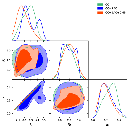
Now we will report the results that we have obtained from the observational data analysis of the models with the different data-sets. Here we have reported the best-fit values of the free parameters along with the minimized $\chi^{2}$ value for all the data-sets in the tabular form.As mentioned earlier, we have used the publicly available CosmoMC (Lewis et al. 2000; Lewis & Bridle 2002) for visualization and subsequent analysis. Using CosmoMC, we calculated the bounds of the free parameters in $68\%$, $95\%$ and $99\%$ confidence intervals and generated 1D distributions as well as 2D joint likelihood contours for the free parameters.The distributions and the likelihood contours are generated for all the three data-sets and depicted by different colours in the figures. The different confidence levels are represented by different shades of the same colour.

3.6.1 Constraints on Model-I

For this model we have taken $m=1$ and performed the fitting analysis. The results are reported below in Tables 1 and 2.

Data	$\lambda$	$\alpha$	$\beta$	${\chi^{2}_{min}}$
CC	$-2.8571~{}or~{}-2.2857$	$2.7143$	$-0.3469~{}or~{}-0.3061$	$6.1$
CC+BAO	$-3.3061$	$2.1428$	$-0.4285$	$47.6055$
CC+BAO+CMB	$-2.0816$	$1.8163$	$0.8367$	$6783.9509$

Table 1: The best fit values of $\lambda$, $\alpha$ and $\beta$, when $m=1$ for Model-I, with the minimum values of $\chi^{2}$

Parameter	68% limits	95% limits	99% limits
$\lambda$	$-2.93^{+0.87}_{-0.43}$	$-2.93^{+0.91}_{-1.0}$	$-2.93^{+0.99}_{-1.1}$
$\alpha$	$1.82^{+0.41}_{-0.79}$	$1.82^{+1.1}_{-0.87}$	$1.82^{+1.2}_{-0.98}$
$\beta$	$-0.07^{+0.16}_{-0.26}$	$-0.07^{+0.41}_{-0.34}$	$-0.07^{+0.53}_{-0.40}$
$\lambda$	$-3.00^{+0.59}_{-0.59}$	$-3.00^{+0.96}_{-0.96}$	$-3.00^{+1.0}_{-1.0}$
$H$	$72.40^{+0.58}_{-0.58}$	$72.40^{+0.96}_{-0.96}$	$72.40^{+1.0}_{-1.0}$
$\Omega_{m0}$	$0.30^{+0.12}_{-0.12}$	$0.30^{+0.19}_{-0.19}$	$0.30^{+0.20}_{-0.20}$

Table 2: Bounds on the free parameters from CC data for different confidence limits

Figure 1: 1D distributions and 2D joint likelihood contours of the free parameters ($\lambda,\alpha,\beta$) of Model I. The deeper shades show the $68\%$ confidence intervals and the lighter shades represent the $95\%$ confidence intervals for the parameters. The figure on the right panel shows the likelihood contours for the present day matter density parameter $\Omega_{m0}$ and present day value of Hubble parameter $H$.

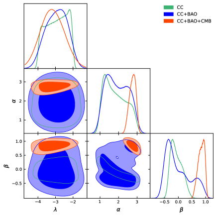
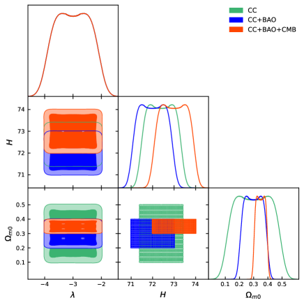
From Fig.1, it is evident that the distributions of the free parameters are quite skewed compared to Gaussian distribution. For the free parameter $\lambda$, we clearly see that it’s distribution is perfectly Gaussian centred around $-3$ for CC+BAO+CMB dataset. But for the other datasets the centre shifts to the right and moreover the Gaussian nature is distorted. In case of $\alpha$ we see that for CC+BAO+CMB data-set the distribution is Gaussian around $2.8$. For the other data-sets the distribution is distorted and the centre shifts towards the left. The distribution of $\beta$ is not perfectly Gaussian for any date-set. But for CC+BAO+CMB it is nearly Gaussian around 0.8. The centre shifts towards left for the other data-sets. The different confidence levels of the free parameters are shown in the contours using different shades. From the contours we see that the parameter limits obtained for CC+BAO data-sets are the least constrained and those for CC+BAO+CMB are most constrained. The constrained values for the parameters $\Omega_{m0}$ and $H$ presented in the table 2 are obtained in the acceptable range according to the recent cosmological observations.

3.6.2 Constraints on Model-II

In this model we have fixed $m=1$ and performed the fitting analysis. The results are summarized in the following tables, viz., 3 and 4.

Data	$\lambda$	$\alpha$	$\beta$	${\chi^{{}^{2}}_{min}}$
CC	$-0.0082$	$0.6836$	$49.7959$	$7.1$
CC+BAO	$-0.0041$	$0.8469$	$-0.4285$	$55.9183$
CC+BAO+CMB	$-9.9e-05$	$0.5102$	$53.0612$	$6640.0877$

Table 3: The best fit values of $\lambda$, $\alpha$ and $\beta$, when $m=1$ for Model-II, with the minimum values of $\chi^{2}$

Parameter	68% limits	95% limits	99% limits
$\lambda$	$-0.102^{+0.058}_{-0.0.058}$	$-0.102^{+0.094}_{-0.094}$	$-0.102^{+0.098}_{-0.098}$
$\alpha$	$0.74^{+0.11}_{-0.13}$	$0.74^{+0.23}_{-0.21}$	$0.74^{+0.26}_{-0.24}$
$\beta$	$49.97^{+5.98}_{-5.98}$	$49.99^{+9.88}_{-9.88}$	$49.99^{+9.91}_{-9.91}$
$\lambda$	$-1.00^{+0.59}_{-0.59}$	$-1.00^{+0.96}_{-0.96}$	$-1.00^{+1.0}_{-1.0}$
$H$	$72.60^{+0.35}_{-0.35}$	$72.60^{+0.58}_{-0.58}$	$72.60^{+0.60}_{-0.60}$
$\Omega_{m0}$	$0.35^{+0.029}_{-0.029}$	$0.35^{+0.048}_{-0.048}$	$0.35^{+0.050}_{-0.050}$

Table 4: Bounds on the free parameters from CC data for different confidence limits

Figure 2: 1D distributions and 2D joint likelihood contours of the free parameters ($\lambda,\alpha,\beta$) of Model II. The deeper shades show the $68\%$ confidence intervals and the lighter shades represent the $95\%$ confidence intervals for the parameters. The figure on the right panel shows the likelihood contours for the present day matter density parameter $\Omega_{m0}$ and present day value of Hubble parameter $H$.

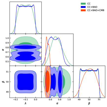
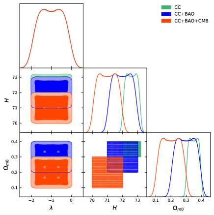
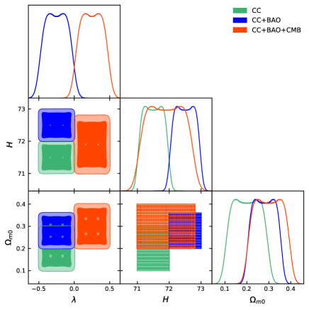
Figure 2 represents the confidence contours for this model. From the distribution plots of the free parameters we see that the distributions are highly skewed compared to the Gaussian distribution. For $\lambda$ there is no proper peak of the distribution and there is no well defined distribution for the CC+BAO+CMB case. For $\alpha$, the distributions are comparatively smoother with a proper Gaussian centred at $0.74$ for the CC data set. For the other data-sets there are significant distortions evident from the plots. Finally for $\beta$ we see that the distributions for CC and CC+BAO are almost identical. The distribution for CC+BAO+CMB is comparatively skewed towards the right. Moreover the contours involving $\lambda$ does not show the case for CC+BAO+CMB. This is probably due to computational complicacy of the model. Due to the involvement of the exponential function probably there is no real limit for $\lambda$ for this data-set. Unlike the previous model here we see that the contours for CC data-set are least constrained and those for CC+BAO+CMB (for $\alpha$ only) are the most constrained scenarios.

3.6.3 Constraints on Model-III

Now, we will turn our focus on model-III. Unlike Model-I and Model-II, here, we did not require to fix any free parameters since the number of free parameters are quite less and manageable. In the tables 5 and 6, the details of the results are summarized.

Data	$\lambda$	$f0$	$m$	${\chi^{2}_{min}}$
CC	$0.3332$	$-1.8775$	$0.3387$	$5.4$
CC+BAO	$0.6969$	$-1.1836$	$0.7244$	$33.1537$
CC+BAO+CMB	$0.1716$	$-1.6122$	$0.1734$	$6191.3833$

Table 5: The best fit values of $\lambda$, $f0$ and $m$ for Model-III, with the minimum values of $\chi^{2}$

Parameter	68% limits	95% limits	99% limits
$\lambda$	$0.273^{+0.070}_{-0.11}$	$0.27^{+0.30}_{-0.18}$	$0.27^{+0.34}_{-0.22}$
$f0$	$-1.42^{+0.38}_{-0.25}$	$-1.42^{+0.48}_{-0.56}$	$-1.42^{+0.56}_{-0.66}$
$m$	$0.286^{+0.062}_{-0.098}$	$0.29^{+0.31}_{-0.19}$	$0.29^{+0.32}_{-0.21}$
$\lambda$	$0.25^{+0.15}_{-0.15}$	$0.25^{+0.24}_{-0.24}$	$0.25^{+0.25}_{-0.25}$
$H$	$73.0^{+0.58}_{-0.58}$	$73.0^{+0.96}_{-0.96}$	$73.0^{+1.0}_{-1.0}$
$\Omega_{m0}$	$0.40^{+0.12}_{-0.12}$	$0.40^{+0.19}_{-0.19}$	$0.40^{+0.20}_{-0.20}$

Table 6: Bounds on the free parameters from CC data for different confidence limits

Figure 3: 1D distributions and 2D joint likelihood contours of the free parameters ($\lambda,f_{0},m$) of Model III. The deeper shades show the $68\%$ confidence intervals and the lighter shades represent the $95\%$ confidence intervals for the parameters. The figure on the right panel shows the likelihood contours for the present day matter density parameter $\Omega_{m0}$ and present day value of Hubble parameter $H$.

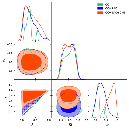
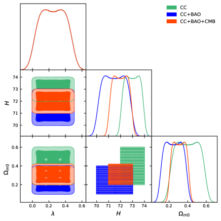
Figure 3 shows the 2D confidence contours and the distributions followed by the free parameters of model-III. From the distribution curves we see that for none of the parameters we get a perfect Gaussian distribution for any data-set. The nearest is the distribution for $m$ for the CC+BAO dataset, which is almost Gaussian in nature with some irregularities in the right wing. The other curves for $m$ are quite skewed on either sides. Similarly the distributions for $\lambda$ are quite skewed compared to a normal curve. The situation for $f_{0}$ is better with bell shaped curves but does not possess a well defined peak. The contours give the ranges of the parameters in 2D scenario for $68\%$ and $95\%$ confidence limits. For this model the most constrained parameter limits are obtained for the CC data-set, which is contrary to the results obtained in the previous models. The least constrained contours are obtained for the CC+BAO+CMB data-set. For this model the constrained value of $\Omega_{m0}$ obtained, is on a little higher side compared to the cosmologically accepted range.

3.6.4 Constraints on Model-IV

Here we will report the results obtained from the analysis for model-IV. The model is fitted with the observational data via the $\chi^{2}$ minimization mechanism and the best fit values of the free parameters are estimated. Ranges of parameters and their confidence contours for different limits are generated using the CosmoMC code. The results are reported in the following tables,7 and 8.

Data	$\lambda$	$f0$	$m$	${\chi^{2}_{min}}$
CC	$0.3265$	$2.6122$	$0.3327$	$2.2$
CC+BAO	$0.1836$	$2.4285$	$0.1002$	$310.1417$
CC+BAO+CMB	$0.1632$	$2.3877$	$0.1775$	$4920.1211$

Table 7: The best fit values of $\lambda$, $f0$ and $m$ for Model-IV, with the minimum values of $\chi^{2}$

Parameter	68% limits	95% limits	99% limits
$\lambda$	$0.258^{+0.11}_{-0.090}$	$0.26^{+0.15}_{-0.17}$	$0.26^{+0.15}_{-0.17}$
$f0$	$2.43^{+0.29}_{-0.34}$	$2.43^{+0.60}_{-0.56}$	$2.43^{+0.75}_{-0.70}$
$m$	$0.266^{+0.11}_{-0.085}$	$0.27^{+0.14}_{-0.17}$	$0.27^{+0.14}_{-0.17}$
$\lambda$	$0.25^{+0.15}_{-0.15}$	$0.25^{+0.24}_{-0.24}$	$0.25^{+0.25}_{-0.25}$
$H$	$72.50^{+0.87}_{-0.87}$	$72.50^{+1.4}_{-1.4}$	$72.50^{+1.5}_{-1.5}$
$\Omega_{m0}$	$0.27^{+0.16}_{-0.16}$	$0.27^{+0.22}_{-0.22}$	$0.27^{+0.24}_{-0.24}$

Table 8: Bounds on the free parameters from CC data for different confidence limits

Figure 4: 1D distributions and 2D joint likelihood contours of the free parameters ($\lambda,f_{0},m$) of Model IV. The deeper shades show the $68\%$ confidence intervals and the lighter shades represent the $95\%$ confidence intervals for the parameters. The figure on the right panel shows the likelihood contours for the present day matter density parameter $\Omega_{m0}$ and present day value of Hubble parameter $H$.

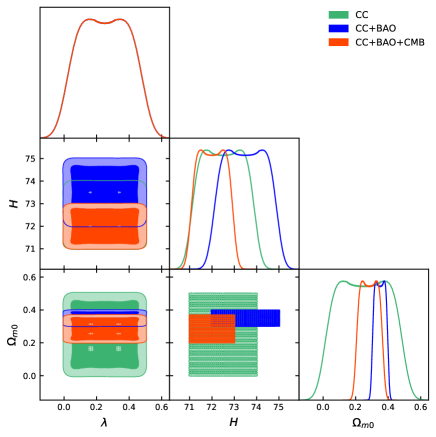
In fig.4 we have generated the 2D confidence contours and the distributions for the free parameters of model-IV. Here the parameter distributions are far more Gaussian like than the previous model. Specially for $f_{0}$ the distributions for CC and CC+BAO+CMB data-sets are perfectly Gaussian with a little difference between the means. For this model the distributions for CC+BAO data-set show the greatest skewness compared to Normal distribution at least for $\lambda$ and $f_{0}$. For $m$ the scenarion is relatively smoother, but not completely devoid of skewness. Here we see that the parameter space is tightly constrained by the CC+BAO+CMB data-set. The other data-sets apply comparatively lighter grips on the parameters.

3.6.5 Constraints on Model-V

Finally, we will report the result of our fifth model here. It is relevant to mention here that this model has some background theoretical motivations and hence the results for this model may be interesting for referencing other results. Here, we have only two free parameters, which is computationally a convenient scenario. The results are given in the tables 9 and 10.

Data	$\lambda$	$\alpha$	${\chi^{2}_{min}}$
CC	$-0.3279$	$0.3941$	$3.84$
CC+BAO	$-0.2014$	$0.1119$	$37.9462$
CC+BAO+CMB	$-0.1862$	$0.0766$	$6447.6411$

Table 9: The best fit values of $\lambda$ and $\alpha$ for Model-V, with the minimum values of $\chi^{2}$

Parameter	68% limits	95% limits	99% limits
$\lambda$	$-0.25^{+0.14}_{-0.14}$	$-0.25^{+0.24}_{-0.24}$	$-0.25^{+0.25}_{-0.25}$
$\alpha$	$0.408^{+0.057}_{-0.045}$	$0.408^{+0.087}_{-0.093}$	$0.408^{+0.092}_{-0.11}$
$\lambda$	$-0.25^{+0.15}_{-0.15}$	$-0.25^{+0.24}_{-0.24}$	$0.25^{+0.26}_{-0.26}$
$H$	$71.50^{+0.29}_{-0.29}$	$71.50^{+0.48}_{-0.48}$	$71.50^{+0.50}_{-0.50}$
$\Omega_{m0}$	$0.20^{+0.059}_{-0.059}$	$0.20^{+0.096}_{-0.096}$	$0.20^{+0.10}_{-0.10}$

Table 10: Bounds on the free parameters from CC data for different confidence limits

Figure 5: 1D distributions and 2D joint likelihood contours of the free parameters ($\lambda,\alpha$) of Model V. The deeper shades show the $68\%$ confidence intervals and the lighter shades represent the $95\%$ confidence intervals for the parameters. The figure on the right panel shows the likelihood contours for the present day matter density parameter $\Omega_{m0}$ and present day value of Hubble parameter $H$.

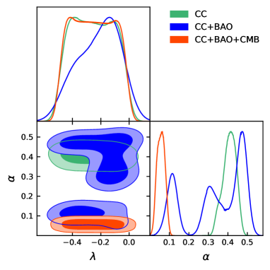
In fig.5 we have shown the 2D confidence contours and the distributions for the free parameters of model-V. We see that both the parameters behave strangely for the CC+BAO data-set. This was seen in the previous model as well. The distribution of $\alpha$ is highly scattered over a large interval for the CC+BAO data-set. This shows that it is very lightly constrained by this data. The results for the other data sets are better. This fact is clearly seen in the contours where the intervals for the CC+BAO data sets are highly de-localized. In fact there are two different ranges at two different levels for the CC+BAO data-set. This is very unique and not seen in any other models. The parameter space is tightly constrained by the CC+BAO+CMB data-set. For this model the constrained value of $\Omega_{m0}$ obtained, is on a little lower side compared to the cosmologically accepted range.

4 Model comparison

Here we will use two model comparison criteria to check our models. They are the Akaike Information Criterion (AIC) (Akaike 1974) and the Bayesian or Schwarz information criterion (BIC) (Schwarz 1978). These are defined as follows,

$$AIC=-2\ln\mathcal{L}+2d=\chi^{2}_{min}+2d$$ (4.1)

and

$$BIC=-2\ln\mathcal{L}+d\ln N=\chi^{2}_{min}+d\ln N$$ (4.2)

where, $\mathcal{L}=\exp{\left(-\chi^{2}_{min}/2\right)}$ is the maximum likelihood function, $d$ is the number of model parameters and $N$ represents the total number of data points in the data used to constrain the model parameters. These model selection criteria involves the number of free parameters used in the model which is a very important fact. This is because we know that a model having more number of free parameters has greater degree of freedom to fit an observational data by changing its shape more conveniently. But from the Occam’s Razor we also know that a model with the least number of free parameters is most desirable for solving any problem. So a model with more number of free parameters needs to be imposed with some penalties in order to build up a logical criteria. This idea has been taken into account while building up these statistical relations for model testing. Now since AIC and BIC may take on any positive values, we need to have a reference model with respect to which the selection criteria must be framed. Here we will use the $\Lambda CDM$ model as our reference model in this comparison. So for any model denoted by $M$ we define $\Delta AIC=AIC_{M}-AIC_{\Lambda CDM}$ and $\Delta BIC=BIC_{M}-BIC_{\Lambda CDM}$. Now using this difference parameter we have three cases according to the Jeffrey’s scale.

i) When $\Delta AIC\leq 2$ or $\Delta BIC\leq 2$, then the model under scrutiny has good support from the reference model.

ii) When $4\leq\Delta AIC\leq 7$ or $4\leq\Delta BIC\leq 7$, then the model has lesser support from the reference model.

iii) When $\Delta AIC\geq 10$ or $\Delta BIC\geq 10$, then the model has no observational data support from the reference model.

Now it must be mentioned that these scales are not exclusive and extreme care must be taken while using these (Nesseris & Garcia Bellido, 2013).

Models	Data-set	AIC	$\Delta$AIC	BIC	$\Delta$BIC
$\Lambda CDM$ Model	CC	20.6068	0	48.216	0
	CC+BAO	55.1533	0	71.3601	0
	CC+BAO+CMB	577.50	0	645.93	0
Model-I	CC	26.14	5.5332	73.6185	25.4025
	CC+BAO	65.3055	10.1522	95.6325	24.2724
	CC+BAO+CMB	650.75	73.25	693.21	47.28
Model-II	CC	24.69	4.0832	75.3081	27.0921
	CC+BAO	69.9487	14.7954	97.3256	25.9655
	CC+BAO+CMB	654.39	76.89	689.92	43.99
Model-III	CC	23.05	2.4432	55.1089	6.8929
	CC+BAO	60.1537	5.0004	82.1141	10.754
	CC+BAO+CMB	597.38	19.88	660.01	14.08
Model-IV	CC	21.26	0.6532	59.9084	11.6924
	CC+BAO	60.5156	5.3623	80.5621	9.202
	CC+BAO+CMB	591.72	14.22	658.73	12.80
Model-V	CC	24.25	3.6432	57.3078	9.0918
	CC+BAO	71.9472	16.7939	82.4562	11.0961
	CC+BAO+CMB	601.44	23.94	662.15	16.22

Table 11: The values for the AIC and BIC criteria for the different models

The values of AIC and BIC criteria for all the models are reported in the Table11. From the table we see that for Model-I, there is good observational support from CC data compared to $\Lambda CDM$ model both from AIC and BIC criteria. But for CC+BAO and CC+BAO+CMB setup there is almost no observational support both according to AIC and BIC. Similarly for all the models there is good support from CC data according to AIC and BIC criteria compared to $\Lambda CDM$ model. Model-II has no support for CC+BAO and CC+BAO+CMB just like Model-I. So Model-I and Model-II are almost similar as far as support from observational data is concerned. This can be attributed to the fact that both involve coupling between matter and curvature in minimal form.

Model-III and IV both involve non-minimal coupling between $R$ and $T$, but the support from observational data according to AIC and BIC criteria are not analogous. We see that for Model-III there is good support from CC+BAO dataset especially according to BIC criteria. But for CC+BAO+CMB setup there is hardly any support. For Model-IV the situation is just the reverse of model-III. Here there is no support from CC+BAO dataset but there is very good support from CC+BAO+CMB dataset for both the criteria. For Model-V we see that there is observational support from CC+BAO according to AIC criterion, but not according to BIC criterion. There is no support from CC+BAO+CMB dataset for this model. So it is seen that all the models are having observational support from some of the data setups but none is having support from all the data types. From this we can conclude that none of the models can be ruled out from this analysis. All are having certain degree of efficiency as far as complying with the observational data is concerned. Moreover looking at the AIC and BIC values it can be concluded that Model-III, IV and V are favoured over the models-I and II. This again confirms the fact that non-minimal coupling is a cosmological favoured set-up. However it should be kept in mind that this is based on the fact that the comparison is done with respect to the $\Lambda CDM$ model which we have considered as the reference model. Taking a different reference or data-set may change our conclusion. However, we believe that our references ($\Lambda CDM$ model and CC data) used here are quite efficient and accepted structures of contemporary cosmology. In such cases, our analysis, results and conclusion should be quite reliable.

5 Conclusion

In this work we have performed an observational data analysis on $f(R,T)$ gravity using the cosmic chronometer data. Five different models of the gravity theory were considered taking into account both minimal and non-minimal coupling between matter and geometry. The first two models were constructed based on minimal coupling using the power law and exponential models. The third model involved pure non-minimal coupling between matter and geometry and the fourth model was the non-minimal coupling model. Finally we picked up the fifth model from the literature which makes it the most motivated model of all the models probed. The first four models were constructed in such a way that they covered almost all mathematical possibilities. This was achieved by keeping the models generic in nature so that all other possibilities will be some limiting or particular cases of these models. We have used the 30 point $z-H(z)$ cosmic chronometer data to constrain the free parameters of these models. We constructed the $\chi^{2}$ statistic using the Hubble parameter value from the data and the theories. We have considered three different data settings namely, CC, CC+BAO and CC+BAO+CMB using which the analysis is done. Adding the BAO and CMB peak parameters with the CC data setting gave an extra edge and helped us to get better constraints on the parameters. Using a minimizing technique we fitted the models with the data and obtained the best fit values of the free parameters of the models. Lesser the minimum $\chi^{2}$ value better is the compliance of the theory with the data. Using the publicly available CosmoMC code we determined the acceptable ranges of the free parameters in the respective models in three different confidence intervals, i.e., $68\%$, $95\%$ and $99\%$ corresponding to the observational data. We have also generated the confidence contours showing these ranges for all the free parameters. The plots also show the general distribution followed by the model parameters. All these have been done for all the three different data-sets as can be seen from the tables and the contours. Values for all the cases have been reported in the paper and corresponding contour plots for all the confidence intervals have been shown. It was seen that different data-sets showed different degree of parameter constraining for different models. Looking at the general distribution followed by the parameters we can easily compare and find out how they vary from the Gaussian distribution. It was seen that most of the cases were skewed compared to the usual normal curve. Finally we have compared the $f(R,T)$ models used in this study with the $\Lambda CDM$ model and checked how much observational support the models enjoy. This is done via a statistical mechanism, where AIC and BIC parameters were calculated and compared. Then using the Jeffrey’s scale we could conclude which models are more efficient. It was seen that the models with non-minimal coupling between matter and curvature are observationally more favoured than the others. This idea which is already present in the literature is re-confirmed from this analysis. It must be mentioned here that none of the models used in this analysis have $\Lambda$CDM cosmology as a limit. This is quite clear from the considerable deviations of the AIC and BIC values of the models in comparison to those of the $\Lambda$CDM model. Moreover this is quite expected from the formulation of the theory, where the matter sector have been coupled with the curvature in the gravity Lagrangian itself. This creates extra force giving rise to non-geodesic motion. The deviation from the standard model is such that, it cannot be recovered as any limiting case of these models. There may be questions regarding the motivations of the models used in this work. So we would like to mention here that these models are not cosmologically motivated (except model V), and neither do they solve any particular issue. But this work is important for the development of $f(R,T)$ theories, especially considering that fact that the models considered here are generic in nature from the mathematical point of view and can cover a family of models as limiting cases. So here we are not solving any cosmological problem, but trying to create viable theories of $f(R,T)$ with support from observational data. These models being observationally constrained and favoured may be used in future works on this theory for solving various cosmological problems. So this work is a significant advancement for $f(R,T)$ theory and modified gravity.

6 Appendix : CC Data

$z$	$H(z)$	$\sigma(z)$	$z$	$H(z)$	$\sigma(z)$
0.07	69	$\pm$ 19.6	0.4783	80.9	$\pm$ 9
0.09	69	$\pm$ 12	0.48	97	$\pm$ 62
0.12	68.6	$\pm$ 26.2	0.593	104	$\pm$ 13
0.17	83	$\pm$ 8	0.68	92	$\pm$ 8
0.179	75	$\pm$ 4	0.781	105	$\pm$ 12
0.199	75	$\pm$ 5	0.875	125	$\pm$ 17
0.2	72.9	$\pm$ 29.6	0.88	90	$\pm$ 40
0.27	77	$\pm$ 14	0.9	117	$\pm$ 23
0.28	88.8	$\pm$ 36.6	1.037	154	$\pm$ 20
0.352	83	$\pm$ 14	1.3	168	$\pm$ 17
0.3802	83	$\pm$ 13.5	1.363	160	$\pm$ 33.6
0.4	95	$\pm$ 17	1.43	177	$\pm$ 18
0.4004	77	$\pm$ 10.2	1.53	140	$\pm$ 14
0.4247	87.1	$\pm$ 11.2	1.75	202	$\pm$ 40
0.44497	92.8	$\pm$ 12.9	1.965	186.5	$\pm$ 50.4

Table 12: Cosmic Chronometer 30 point Data Set (Moresco, 2015). It shows the 30 point cosmic chronometer $z-H(z)$ data with the standard error $\sigma(z)$

References

-
[1]
Akaike H., 1974 IEEE Trans. Automat. Contr. 19, 716.
Alvarenga F. G., A. de la Cruz-Dombriz, Houndjo M. J. S., Rodrigues M. E., S ez-G mez D., 2013 PRD 87, 10, 103526.
Amendola L., 1999 PRD 60, 043501.
Amendola L., Polarski D., Tsujikawa S., 2007, PRL, 98, 131302
Amendola L., Gannouji R,. Polarski D., Tsujikawa S., 2007, PRD, 75, 083504
Azevedo R. P. L., Pramos J., 2016 PRD 94, 064036.
Azizi T., Yaraie E., 2014, IJMPD, 23, 1450021
Bertolami O., Frazo P., Pramos J., 2010 PRD 81, 104046.
Bertolami O., Pramos J., 2010 JCAP 03, 009 .
Bertolami O., Pramos J., 2011 PRD 84, 064022.
Bertolami O., Frazo P., Pramos J., 2011 PRD 83, 044010.
Bertolami O., Frazo P., Pramos J., 2013 JCAP 05, 029.
Brax P., 2018, Rep. Prog. Phys., 81, 1
Das A., Ghosh S., Guha B. K., Das S., Rahaman F., 2017 PRD 95, 12, 124011.
De Felice A., Tsujikawa S., 2010, Living. Rev. Relativ. 13, 3.
Fakir R., Unruh W. G., 1990 PRD 41, 1783 .
Futamase T., Maeda K. I., 1989 PRD 39, 399.
Ghose S., Thakur P., Paul B. C., 2012, MNRAS, 421, 20
Harko T., 2010 PRD 81, 084050.
Harko T., Lobo F. S. N., 2010 EPJC 70, 373.
Harko T., Lobo F. S. N., Nojiri S., Odintsov S. D., 2011, PRD 84, 024020.
Jimenez R., Loeb A., 2002, ApJ, 573, 37
Komatsu E., et al., 2011, Astrophys. J. Suppl. Ser. 192, 18.
Landau L. D., Lifshitz E. M., 1998 The Classical Theory of Fields (Butterworth-Heinemann, Oxford).
Lewis A., Challinor A., Lasenby A., 2000 ApJ. 538, 473.
Lewis A., Bridle S., 2002 PRD 66, 103511.
Moresco M., 2015, MNRAS, 450, 1
Nesseris S., (2009) PRD 79, 044015 .
Nesseris S., Garc ia-Bellido J., 2013 JCAP, 2013, 036.
Nojiri S., Odintsov S. D., 2006, PRD, 74, 086005
Nojiri S., Odintsov S. D., 2007, Int. J. Geom. Meth. Mod. Phys., 4, 115
Nojiri S., Odintsov S. D., Oikonomou V. K., 2017, Phys. Rept., 692, 1
Paul B. C., Thakur P., Ghose S., 2010, MNRAS, 407, 415
Paul B. C., Ghose S., Thakur P., 2011, MNRAS, 413, 686
Perlmutter S. et al., 1999, ApJ, 517, 565
Pourhassan B., Rudra P., 2020 PRD 101, 084057.
Riess A. G. et al., 1998, AJ, 116, 1009
Rudra P., 2015 EPJP 130, 4, 66.
Rudra P., 2020 Arxiv : 2006.00228 [gr-qc].
Schwarz G. E., 1978 Annals Statist. 6, 461.
Shabani H., Farhoudi M., 2013 PRD 88, 044048.
Sharif M., Zubair M., 2012 JCAP 03, 028.
Sharif M., Siddiqa A., 2019 GRG 51, 6, 74.
Simon J., Verde L., Jimenez R., 2005, PRD, 71, 123001
Song Y-S., Hu W., Sawicki I., 2007, PRD, 75, 044004
Sotiriou T. P., Faraoni V., 2010, Rev. Mod. Phys., 82, 451.
Spergel D. N. et al., 2003, ApJS, 148, 175
Stern D., Jimenez R., Verde L., Kamionkowski M., Stanford S., 2010, JCAP, 02, 008
Thakur P., Ghose S., Paul B. C., 2009, MNRAS, 397, 1935
Thakur S., Sen A. A., 2013 PRD 88, 044043.
Torres D. F., 2002 PRD 66, 043522.
Uzan J. P., 1999 PRD 59, 123510.
Wu P., Yu H. W., 2007, PLB, 644, 16
Zaregonbadi R., Farhoudi M., Riazi N., 2016 PRD 94, 084052.
Zhang C., Zhang H., Yuan S., Zhang T.-J., Sun Y.-C., 2014, Res. Astron. Astrophys., 14, 10