High metal content of highly accreting quasars

Abstract

We present an analysis of UV spectra of 13 quasars believed to belong to extreme Population A (xA) quasars, aimed at the estimation of the chemical abundances of the broad line emitting gas. Metallicity estimates for the broad line emitting gas of quasars are subject to a number of caveats, xA sources with the strongest Feii emission offer several advantages with respect to the quasar general population, as their optical and UV emission lines can be interpreted as the sum of a low-ionization component roughly at quasar rest frame (from virialized gas), plus a blueshifted excess (a disk wind), in different physical conditions. Capitalizing on these results, we analyze the component at rest frame and the blueshifted one, exploiting the dependence of several intensity line ratios on metallicity $Z$. We find that the validity of intensity line ratios as metallicity indicators depends on the physical conditions. We apply the measured diagnostic ratios to estimate the physical properties of sources such as density, ionization, and metallicity of the gas. Our results confirm that the two regions (the low-ionization component and the blue-shifted excess) of different dynamical conditions also show different physical conditions and suggest metallicity values that are high, and probably the highest along the quasar main sequence, with $Z\sim 20-50Z_{\odot}$, if the solar abundance ratios can be assumed constant. We found some evidence of an overabundance of Aluminium with respect to Carbon, possibly due to selective enrichment of the broad line emitting gas by supernova ejecta.

1 Introduction

Thanks to large public databases as the Sloan Digital Sky Survey (SDSS) catalogs, we have unrestricted access to a large wealth of astronomical data (for example, several editions of quasar catalogues, Schneider et al. 2010; Pâris et al. 2017, and of value-added measurements by Shen et al. 2011). SDSS spectra of high redshift quasars ($z\gtrsim$ 2) cover the rest frame UV spectral range. It is known since the 1970s that measurements of UV emission lines can be used to explore the physical and chemical properties of active galactic nuclei (AGN). Landmark papers provided the basic understanding of line formation processes due to photoionization (e.g., Wills & Netzer, 1979; Davidson & Netzer, 1979; Baldwin et al., 2003).

The chemical composition of the line emitting gas is an especially intriguing problem from the point of view of the evolution of cosmic structures, but also from the technical side. Nagao et al. (2006b) investigated BLR metallicities using various emission-line flux ratios and claimed that the typical metallicity of the gas in that region is at least super-solar, with typical $Z\sim 5Z_{\odot}$. Moreover, studies of metallicity-redshift dependence (Nagao et al., 2006b; Juarez et al., 2009) show a lack of metallicity evolution up to $z\approx 5$. Similar results are obtained for (Nagao et al., 2006a). The highest-redshift quasars ($z\gtrsim 5$ Bañados et al. 2016, e.g.,; Nardini et al. 2019, e.g.,) are known to show UV spectra remarkably similar to the ones observed at low-redshift, especially the ones accreting at high rate and radiating at high Eddington ratio (Diamond-Stanic et al., 2009; Plotkin et al., 2015; Sulentic et al., 2017). Perhaps surprisingly, these sources are suspected to have high metal content in their line emitting gas, due to the consistent values of several diagnostic ratios measured in quasars with similar spectral properties at low and high z (Martínez-Aldama et al., 2018), and indicating highly super-solar metal content.

Several techniques are applied to estimate the chemical composition in Galactic nebulae (see e.g., Feibelman & Aller 1987 for planetary nebulae). Classical techniques used for Hii and other nebulæ (including the Narrow Line Regions, NLRs) are unfortunately not applicable to the broad line regions of quasars. Permitted and inter-combination lines are too broad to resolve fine structure components of doublets; line profiles are composites and may originate in regions that are spatially unresolved, and unresolved or only partially resolved in radial velocity as well.

However, quasar emission line profiles still offer important clues in the radial velocity domain. The shape of the profile is strongly dependent on the ionization potential of the ionic species from which the line is emitted: it is expedient to subdivide the broad lines in low- and high ionization lines (LILs and HILs). The LIL group in the spectral range under analysis (1200 Å – 2000 Å) includes the following lines: Siii$\lambda$1263, Siii$\lambda$1814, Alii$\lambda$1671, Aliii$\lambda$1860, Siiii]$\lambda$1892, Ciii]$\lambda$1909. High ionization lines are Niv]$\lambda$1486, Oiv]$\lambda$1402, Civ$\lambda$1549, Siiv$\lambda$1397, Oiii]$\lambda$1663, and Heii$\lambda$1640  (for detailed discussion see Collin-Souffrin et al., 1988; Collin-Souffrin & Lasota, 1988; Gaskell, 2000). The Aliii, Siiii], and Ciii] lines sometimes referred to as “intermediate ionization lines:” even if they are mainly produced within the fully ionized region of the emitting gas clouds (Negrete et al., 2012), the ionization potential of their ionic species is closer to the ones of the LILs, and typically $\lesssim 20$ eV.

The two groups of lines (HILs and LILs) do not only show different kinematic properties (Sulentic et al., 1995), but their emission is also likely to occur in fundamentally different physical conditions (Marziani et al., 2010). The HILs are characterized also by the evidence of strong blueshifted emission, very evident in Civ (e.g., Sulentic et al., 2007; Richards et al., 2011; Coatman et al., 2016). Therefore, a careful line comparison/decomposition is necessary, lest inferences may be associated with a non-existent region with inexplicable properties.

The interpretation of two line components involves a virialized region, of relatively low ionization (hereafter referred to the virialized, low-ionization BLR associated with a symmetric broad component, BC), possibly including emission from the accretion disk, and a region of higher ionization, associated with a disk wind or a clumpy outflow, a scenario first proposed by Collin-Souffrin et al. (1988, and further developed by ), and observationally supported by reverberation mapping (e.g., Peterson & Wandel, 1999) and the apparent lack of correlation between HILs and LILs in luminous quasars (e.g., Mejía-Restrepo et al., 2016; Sulentic et al., 2017). Even if all lines were emitted by a wind (Murray et al., 1995; Murray & Chiang, 1997; Proga, 2007a), the conditions at the base of the textcolorwind may strongly differ from the ones downstream in the outflow.

While each UV metal line contains information related to composition (Hamann & Ferland, 1992), not all of the lines listed above can be used in practice. For instance, the Nv and Siii$\lambda$1263 lines are strongly affected by blending with Ly$\alpha$; other lines such as Siii$\lambda$1814 and Niv]$\lambda$1486 are usually weak and require high S/N to be properly measured. The choice of diagnostic ratios used for metallicity estimates will be a compromise between S/N, easiness of deblending, and straightforwardness of physical interpretation. In practice, apart from Ly$\alpha$, only the strongest broad features will be considered as potential metallicity estimators in this work (Sect. 3). The ratio (Siiv+Oiv])/Civ has been widely used in past studies (Hamann & Ferland, 1999, and references therein); this ratio is relatively easy to measure and seems to be the most stable ratio against distribution of gas densities and ionization parameter in the BLR (Nagao et al., 2006b). The ratios involving NV$\lambda 1240$, like Nv/Civ are sensitive to ionization parameter and to nitrogen abundance (e.g Dietrich et al., 2003; Wang et al., 2012a). We will rediscuss the use of these ratios in the context of the xA quasar spectral properties (Sect. 5.8).

Both physical conditions and chemical abundances vary along the quasar main sequence (see e.g., Sulentic et al., 2000b; Kuraszkiewicz et al., 2009; Shen & Ho, 2014; Wildy et al., 2019; Panda et al., 2020b). Solar and even slightly subsolar values are possible toward the extreme Population B, where Feii emission is often undetectable above noise (e.g., Hamann et al., 2002; Punsly et al., 2018). At the other extreme, where Feii is most prominent, estimates suggest $Z\gtrsim 10Z_{\odot}$ (Panda et al., 2018, 2019). Baldwin et al. (2003) derived $Z\approx 15Z_{\odot}$, although in the particular case of a “nitrogen-loud” quasars. Apart from the extremes, it is not obvious whether there is a continuous systematic trend along the sequence. Previous estimates consistently suggest super-solar metallicity up to $Z\lesssim 10$ $Z_{\odot}$ (Warner et al., 2004). Other landmark studies consistently found super-solar metallicity: Hamann & Ferland (1992) derived $Z$ up to $\lesssim 15Z_{\odot}$; Nagao et al. (2006b) found typical values $Z\approx 5Z_{\odot}$, with $Z\sim 10Z_{\odot}$ for the most luminous quasars from the (Siiv+Oiv])/Civ ratio. Sulentic et al. (2014) inferred a large dispersion with the largest value in excess of $10Z_{\odot}$. Similar results were reached by Shin et al. (2013) whose Siiv+Oiv]/Civ ratio measurements suggested $Z\gtrsim 10Z_{\odot}$.

Most interesting along the quasar main sequence are the high accretors. They are selected according to empirical criteria (e.g., Wang et al., 2013; Marziani & Sulentic, 2014; Wang et al., 2014; Du et al., 2016a), and defined by having $R_{\mathrm{FeII}}$$>$ 1, that is with the Feii$\lambda$4570 blend on the blue side of H$\beta$ (as defined by Boroson & Green 1992) flux exceeding the flux of H$\beta$. In the optical diagram of the quasar main sequence (Sulentic et al., 2000b; Shen & Ho, 2014) they are at the extreme tip in terms of Feii prominence, and identified as extreme Population A (hereafter xA), following Sulentic et al. (2002). Depending on redshift, we look for high accretors using different criteria. In case of z $\gtrsim$ 1, it is expedient to use a criterion based on two UV line intensity ratios:

• Aliii/Siiii]$>$ 0.5

• Ciii]/Siiii]$<$ 1.0,

following (Marziani & Sulentic, 2014). These criteria are met by the sources identified as xA Population by Sulentic and collaborators. xA quasars are radiating at the highest luminosity per unit mass, and, at low $z$ they are characterized by relatively low black hole masses for their luminosities and high Eddington ratios (Mathur, 2000; Sulentic et al., 2000a). There is evidence that xA sources tend to have high-metallicity (Shemmer et al., 2004; Martínez-Aldama et al., 2018). Similar properties have been identified as characteristic of narrow-line Seyfert 1 galaxies (NLSy1s) with strong Feii emission. NLS1s also have unusually high metallicities for their luminosities. Shemmer & Netzer (2002) have shown that NLSy1s deviate significantly from the nominal relationship between metallicity and luminosity in AGN. As several studies distinguish between NLSy1s and “broader-lined” AGN, we remark here that all Feii strong NLSy1s meeting the selection criterion $R_{\mathrm{FeII}}$$>1$ are extreme Pop. A sources.

The aim of this work is to investigate the metallicity-sensitive diagnostic ratios of the UV spectral range for extreme Population A quasars i.e., for highly accreting quasars. Section 2 defines our sample, and provides some basic information. In Sect. 3 we define the diagnostic ratios, and describe the basic observational results. In Section 4 we compare measured diagnostic ratios and we compare them with the ones obtained from photoionization simulations. In Sect. 5 we discuss our results in terms of method caveats, metal enrichment, accretion parameters and their implications on the nature of xA sources. We show the UV spectra in Appendix A along with the multicomponent fit analysis of the emission blends, and in the Appendix B we show the trend of $Z$-sensitive ratios as a function of ionization parameter, density, and metallicity.

2 Sample

2.1 Sample definition

Qualitatively, extreme Pop. A objects show prominent Aliii and weak or absent Ciii] emission lines. In general, they show low emission line equivalent widths ($\approx\frac{1}{2}$ of them meet the $W$(Civ)$\lesssim$ 10 Å, and qualify as weak-lined quasars following Diamond-Stanic et al. 2009), and a spectrum that is easily recognizable even by a visual inspection, also because of the “trapezoidal” shape of the Civ profile and the intensity of the $\lambda$1400 blend, comparable to the one of Civ  (Martinez-Aldama et al., 2018).

xA sources were selected according to the criteria given in Sect. 1, using line measurements automatically obtained by the splot task with a cursor script within the IRAF data reduction package. We focus on the spectral range from $\approx$ 1200 Å to 2100 Å, where (1) UV lines used for xA identification are present; (2) the strongest emission features helpful for metallicity diagnostics are also located. The Ly$\alpha$ + Nv blend is usually too heavily compromised by absorptions which make it impossible to reconstruct the emission components especially for Ly$\alpha$. We will make some consideration on the mean strength of the Nv with respect to Civ and Heii$\lambda$1640 (Sect. 5.3), but will not consider Nv as a diagnostics. We selected SDSS DR12 spectra in the redshift range 2.15 $<$ z $<$ 2.40, relatively bright ($r<19$) to ensure moderate-to-high S/N in the continua (in all cases S/N $\gtrsim 5$ in the continuum, and the wide majority with S/N $\gtrsim 10$), and of low declination $\delta<10$. The redshift range was chosen to allow for the possibility of H$\beta$ coverage in the $H$ band by eventual near-IR spectroscopic observations. The DR12 sample selected with these criteria is $\approx$ 500 sources strong. xA sources were selected out of this sample with an automated procedure, inspected to avoid broad absorption lines, and further vetted for obtained a small pilot sample of $\sim 10$ sources. A larger sample of xA sources will be considered in a subsequent work (Garnica et al., in preparation). The final selection includes 13 sources. With the adopted selection criteria in flux and redshift, we expect a small dispersion in the accretion parameters (especially luminosity; Sect. 5.2). Indeed, the selected sources are rather homogeneous in terms of spectral appearance, with a few sources included in our sample that however show borderline criteria. They will be considered is Sect. 4.1.1 in terms of their individual $U$, $n_{\mathrm{H}}$.

2.2 Sample properties

Table 1 provides basic information for the 13 sources of our sample: SDSS name, redshift from the SDSS, the difference between our redshift estimation using Aliii  (described in 3.1) and the SDSS redshift $\delta z$ = $z-z_{\mathrm{SDSS}}$, the $g$-band magnitude provided by Adelman-McCarthy et al. (2008a), the $g-r$ color index, the rest-frame-specific continuum flux at 1700 Å and 1350 Å measured on the rest frame, the S/N at 1450 Å. All other sources were covered by the FIRST (Becker et al., 1995), but undetected. Considering that the typical rms scatter of FIRST radio maps is $\approx$0.15 Jy, and the typical fluxes of in the $g$ band, we have upper limits $\lesssim 5$ in the radio-to-optical ratio, qualifying the sample sources as radio quiet. Distances were computed using the formula provided by Sulentic et al. (2006, their Eq. B.5), and $\Lambda$CDM cosmology ($\Omega_{\Lambda}=0.7,\Omega_{\mathrm{M}}=0.3,H_{0}=70$ km s^-1 Mpc^-1). The bolometric luminosity is around $\sim 10^{47}$ erg s^-1, assuming a bolometric correction B.C.₁₃₅₀ = 3.5 (Richards et al., 2006). The sample rms is just $\approx 0.2$ dex: all sources are in a narrow range of distances and have observed fluxes within a factor $\approx$ 2 from their average. This is, in principle, an advantage for the estimation of the physical parameters such as $L/L_{\rm Edd}$, considering the large uncertainty and serious biases associated with the estimation of $M_{\rm BH}$ from UV high-ionization lines. Accretion parameters will be discussed in Sect. 5.2.

Table 1: Source identification and basic properties

SDSS NAME	$z_{\mathrm{SDSS}}$	$\delta z$	${g}$	$g-r$	$f_{\lambda}$(1700 Å)	$f_{\lambda}$(1350 Å)	S/N
(1)	(2)	(3)	(4)	(5)	(6)	(7)	(8)
J010657.94-085500.1	2.355	0.006	18.18	0.095	662	951	20
J082936.30+080140.6	2.189	0.008	18.366	0.302	672	939	11
J084525.84+072222.3	2.269	0.017	18.204	0.331	668	989	13
J084719.12+094323.4	2.295	0.004	18.940	0.234	368	511	17
J085856.00+015219.4	2.160	0.002	17.916	0.255	709	1204	21
J092641.41+013506.6	2.181	0.004	18.591	0.337	377	670	21
J094637.83-012411.5	2.212	0.002	18.561	0.178	385	595	18
J102421.32+024520.2	2.319	0.008	18.49	0.177	478	694	23
J102606.67+011459.0	2.253	0.003	18.982	0.206	428	525	13
J114557.84+080029.0	2.338	0.009	18.545	0.369	243	360	5
J150959.16+074450.1	2.255	0.008	18.938	0.278	223	346	9
J151929.45+072328.7	2.394	0.008	18.662	0.171	405	507	19
J211651.48+044123.7	2.352	0.000	18.825	0.220	404	573	32

Note. — Columns are as follows: (1) SDSS coordinate name; (2) SDSS redshift; (3) correction to redshift estimated in the present work ($\delta z$ = $z-z_{\mathrm{SDSS}}$); (4) $g$-band magnitude from Adelman-McCarthy et al. (2008b); (5) color index $g-r$; (6) continuum flux measured at 1700 Å in units of 10^-17 erg s ^-1 cm ^-2 Å^-1; (7) continuum flux measured at 1350 Å in the same units; (8) S/N measured at continuum level at 1450 Å.

3 Methods

3.1 Redshift determination

The estimate of the quasar systemic redshift in the UV is not trivial, as there are no low-ionization narrow lines available in the spectral range (Vanden Berk et al., 2001). In practice, one can resort to the broad LIL. Negrete et al. (2014) and Martínez-Aldama et al. (2018) consider the Siii$\lambda$1263 and Oi$\lambda$1302 lines to obtain a first estimate. A re-adjustment is then made from the wavelength of the Aliii doublet which is found, in almost all cases, to have a consistent redshift. To determine the Aliii shift those authors used multicomponent fits with all the lines in the region of the blend $\lambda$1900 included. The peak of Aliii  is clearly visible in the spectra of our sample, since in high accretors emission of Aliii is strong with respect to the other lines in the blend at $\lambda$1900Å. We decided to use only this method for redshift estimation (in Tab. 1) and to measure the peak we use single Gaussian fitting from the splot task of the Aliii doublet and/or of the Siiii] line, depending on which feature is sharper. The obtained values are usually $\geq z_{\mathrm{SDSS}}$  (Table 1). This is not a surprise as $z_{\mathrm{SDSS}}$ is based on lines that are mainly blueshifted in xA sources, and hence is a systematic underestimation of the unbiased redshift.

3.2 Diagnostic ratios sensitive to $U$, density, $Z$

Line ratios are sensitive to different parameters. In the UV range, three groups of diagnostic ratios are defined in the literature (e.g. Negrete et al., 2012; Martinez-Aldama et al., 2018).

• Civ/Siiv+Oiv], Civ/Heii have been widely applied as metallicity indicators (e.g., Shin et al., 2013). In principle, Civ/Heii and Siiv/Heii should be sensitive to C and Si abundance because the He abundance relative to Hydrogen can be considered constant. The ionization potentials of C²⁺ and He⁺ are similar. The main difference is that the Heii line is a recombination line, equivalent to Hi H$\alpha$, and the regions where they are formed are not coincident (see Fig. 4).

• Ratios involving Nv, Nv/Civ and Nv/Heii have been also widely used in past work, after it was noted that the Nv line was stronger than expected in a photoionization scenario (e.g., Osmer & Smith, 1976). A selective enhancement of nitrogen (Shields, 1976) is expected due to secondary production of N by massive and intermediate mass stars, yielding [N/H]$\propto Z^{2}$ (Vila-Costas & Edmunds, 1993; Izotov & Thuan, 1999). This process might be especially important at the high metallicities inferred for the quasar BLR. Therefore estimates based on Nv may differ in a systematic way from estimates based on other metal lines (e.g., Matsuoka et al., 2011). In the present sample of quasars, contamination by narrow and semi-broad absorption is severe, and even if we model precisely the high ionization lines, it might be impossible to reconstruct the unabsorbed profile of the red wing of Ly$\alpha$. In addition, S/N is not sufficient to allow for a careful measurement of Niv]$\lambda$1486 and Niii]$\lambda$1750 lines. We defer the systematic analysis of nitrogen lines to a subsequent work, while discussing the consistency of the Nv measures in a high-$Z$ scenario (Sect. 5.3).

• The ratios Aliii/Siiii] and Siiii]/Ciii] are sensitive to density, as the ratios involve intercombination lines with a well defined critical density ($n_{\mathrm{c}}\sim 10^{10}$ cm^-3 for Ciii] (Hamann et al., 2002) and $n_{\mathrm{c}}\sim$ 10¹¹ cm^-3 for Siiii] (Negrete et al., 2010)).

• Siiii]/Siiv, Siii$\lambda$1814/Siiii], and Siii$\lambda$1814/Siiv are sensitive to the ionization parameters and insensitive to $Z$, as they are different ionic species of the same element.

Other intensity ratios entail a dependence on metallicity $Z$, but also on ionization parameter $U$ and density $n_{\mathrm{H}}$ (Marziani et al., 2020).

3.3 Line interpretation and diagnostic ratios

The comparison between LILs and HILs has provided insightful information over a broad range of redshift and luminosity  (Corbin & Boroson, 1996; Marziani et al., 1996, 2010; Sulentic et al., 2017; Bisogni et al., 2017; Shen, 2016; Vietri et al., 2018). A LIL-BLR appears to remain basically virialized (Marziani et al., 2009; Sulentic et al., 2017), as the H$\beta$ profile remains (almost) symmetric and unshifted with respect to rest frame even if Civ blueshifts can reach several thousands of km s^-1. In Population A, the lines have been decomposed into two components:

• The broad component (BC), also known as the intermediate component, the core component or the central broad component following various authors (e.g., Brotherton et al., 1994; Popović et al., 2002; Kovačević-Dojčinović & Popović, 2015; Adhikari et al., 2016). The BC is modeled by a symmetric and unshifted profile (Lorentzian for Pop. A; Véron-Cetty et al. 2001; Sulentic et al. 2002; Zhou et al. 2006), and is believed to be associated with a virialized BLR subsystem.

• The blue shifted component (BLUE). A strong blue excess in Pop. A Civ profiles is obvious, as in some Civ profiles – like the one of the xA prototype I Zw1 or high luminosity quasars – BLUE dominates the total emission line flux (Marziani et al., 1996; Leighly & Moore, 2004; Sulentic et al., 2017). For BLUE, there is no evidence of a regular profile, and the fit attempts to empirically reproduce the observed excess emission. BLUE is detected in a LIL such as H$\beta$ at a very low level, and is not strongly affecting FWHM measurements (Negrete et al., 2018).

3.3.1 Broad component

Diagnostic ratios are not equally well measurable for the BC and the BLUE. For the BC, the following constraints and caveats apply:

Civ/, Siiv/, Aliii/ over Heii

Heii is weak but measurable in most of the objects. Ratios such as Civ/Heii$\lambda$1640, Siiv/Heii$\lambda$1640, Aliii/Heii$\lambda$1640 ($U$-dependent) offer $Z$  indicators. Especially for the low-ionization conditions of the BC emitting gas, these ratios are well-behaved (Sect. 3.5 and 3.6) and will form the basis of the $Z$ estimates presented in this paper.

Siiv/Civ

There are problems in estimating the Siiv line intensity: an overestimation might be possible because of difficult continuum placement (see, for example, the case of SDSSJ085856.00+015219.4 (catalog ) in Appendix A). The relative contribution of Siiv to the blend at $\lambda$1400 is unclear (Wills & Netzer, 1979). A strong BC contribution of Oiv]  is unlikely, as this line has a critical density $n_{\mathrm{c}}\sim 10^{10}$ cm^-3 (Zheng, 1988, see also the isophotal contour of Siiv/Oiv] in Appendix B). Our measurements are nonetheless compared to Siiv+ total Oiv] CLOUDY prediction.

Aliii/Siiii]

This ratio is sensitive to density in the low-ionization BLR domain (Negrete et al., 2012). Values Aliii/Siiii]$>$1 are possible if density is higher than 10¹¹ cm^-3, the critical density of Siiii]. We will not use this parameter as a metallicity estimator, although, in principle, for fixed physical conditions (setting $n_{\mathrm{H}}$ and $U$) the Aliii/Siiii] and Siiii]/Ciii] ratios may become dependent mainly on electron temperature and so on metallicity (Sect. 3.5). The ratio of the total emission in the 1900 blend Aliii+Siiii] +Ciii] over Civ has been used as a metallicity estimator (Sulentic et al., 2014). Considering the uncertain contribution of Feiii emission and especially of the Feiii $\lambda$1914 line in the xA spectra, we will not use the total intensity of the $\lambda$1900 blend as a diagnostic.

Civ/Aliii

Biases might be associated with the estimate of the Civ$\lambda$1549_BC especially when BLUE is so prominent that Civ$\lambda$1549_BC  contributes to a minority fraction.

3.3.2 BLUE component

Civ/Heii$\lambda$1640

The Heii$\lambda$1640 BLUE is well-visible merging smoothly with the red wing of Civ. The ratio Civ/Heii$\lambda$1640 might be affected by the decomposition of the blend, leading to an overestimate of the Heii emission. This ratio is in principle sensitive to metallicity. However, the increase is not monotonic at relatively high $U$ (see the panel for Civ/Heii$\lambda$1640 in Fig. 2). The resulting effect is that the Civ/Heii$\lambda$1640 ratio within the uncertainties leaves the $Z$ unconstrained between 0.1 and 100 solar.

Civ/(Oiv] + Siiv)

The blueshifted excess at $\lambda$1400 is ascribed to Oiv + Siiv emission. A significant contribution can be associated with Oiv] and several transitions of Oiv that are computed by CLOUDY (see e.g., Keenan et al., 2002) are especially relevant at high $U$ values and moderately low $n_{\mathrm{H}}$ ($\sim 10^{8}$ cm^-3). The blue side of the line is relatively straightforward to measure for computing Civ/$\lambda 1400$ with a multicomponent fit, although difficult continuum placement, narrow absorption lines, and blending on the blue side make it difficult to obtain a very precise measurement. A total $\lambda$1400 BLUE emission exceeding Civ is possible if, assuming $\log U\gtrsim 0$, $\log$ $n_{\mathrm{H}}$$\gtrsim 9$ [cm^-3], the metallicity value is very high $20\lesssim Z\lesssim 100Z_{\odot}$, (Sect. 3.6).

(Oiv]+Siiv)/Heii$\lambda$1640

By the same token, the Heii$\lambda$1640 overestimation may lead to a lower (Oiv]+Siiv)/Heii$\lambda$1640 ratio.

3.4 Analysis via multicomponent fits

We analyze 13 objects using the specfit task from IRAF (Kriss, 1994). The use of the $\chi^{2}$ minimization is aimed to provide a heuristic separation between the broad component (BC) and the blue component (BLUE) of the emission lines. After redshift correction following the method described in Sect. 3.1, for each source of our sample we perform a detailed modeling using various components as described below, including computation of asymmetric errors (Sect. 3.4.1). As mentioned in Sect. 3.2, in our analysis we consider five diagnostic ratios for the BC: Civ/$\lambda 1400$, Civ/Heii$\lambda$1640, Aliii/Heii$\lambda$1640, $\lambda$1400/Heii$\lambda$1640, $\lambda 1400$/Aliii, and three for the BLUE: Civ/$\lambda 1400$, Civ/Heii$\lambda$1640, $\lambda 1400$/Heii$\lambda$1640. The Civ/Heii$\lambda$1640 is used with care, as it may yield poor constraints. In addition, it is important to stress that, of the five ratios measured on the BC, only three (the ones dividing by the intensity of Heii$\lambda$1640 BC) are independent. We compare the fit results with arrays of CLOUDY (Ferland et al., 2013) simulations for various metallicities and physical conditions (Sect. 3.5).

For each source we perform the multicomponent fitting in three ranges described below. The best fit is identified by the model with the lowest $\chi^{2}$ i.e., with minimized difference between the observed and the model spectrum. Following the data analysis by Negrete et al. (2012), we use the following components:

The continuum

was modeled as a power-law, and we use the line-free windows around 1300 and 1700 Å (two small ranges where there are no strong emission lines) to scale it. If needed, we divide the continuum into three parts (corresponding to the three regions mentioned below). Assumed continua are shown in the Figures of Appendix A.

Feii emission

usually does not contribute significantly in the studied spectral ranges. We consider the Feii template which is based on CLOUDY simulations of Brühweiler & Verner (2008) when necessary. In practice the contamination by the blended Feii emission yielding a pseudo-continuum is negligible. Some Feii  emission lines were detectable in only a few objects and around $\approx$ 1715 Å, at 1785  Å, and at 2020  Å. In these cases, we model them using single Gaussians.

Feiii emission

affects more the 1900 Å region and seems to be strong when AlIII $\lambda$1860 is strong as well (Hartig & Baldwin, 1986). To model these lines we use the template of Vestergaard & Wilkes (2001).

Region 1300 - 1450Å 

is dominated by the Siiv+ Oiv]  high ionization blend with strong blueshifted component. The fainter lines as Siii$\lambda$1306, Oi$\lambda$1304 and Cii$\lambda$1335 are also detectable. For the broad and blueshifted components we use the same model as in case of Civ and Heii$\lambda$1640. This spectral range is often strongly affected by absorption.

Region 1450 - 1700 Å 

is dominated by Civ emission line which we model as a fixed in the rest-frame wavelength Lorentzian profile representing the BC and two blueshifted asymmetric Gaussian profiles vary freely. The same model is used for Heii$\lambda$1640.

Region 1700 - 2200 Å 

is dominated by Aliii, Siiii] and Feiii  intermediate - ionization lines. We model Aliii and Siiii] using Lorentzian profiles, following Negrete et al. (2012). Ciii] emission is also included in the fit, although the dominant contribution around $\lambda 1900$ is to be ascribed to Feiii (Martínez-Aldama et al., 2018, and references therein). We use the template of Vestergaard & Wilkes (2001) to model Feiii emission. No BLUE is ascribed to these intermediate ionization lines.

Absorption lines

are modeled by Gaussians, and included whenever necessary to obtain a good fit.

The fits to the observed spectral ranges are shown in the Figures of Appendix A.

3.4.1 Error estimation on line fluxes

The choice of the continuum placement is the main source of uncertainty in the measurement of the emission line intensities. The fits in Appendix A show that, in the majority of cases, the FWHM of the Aliii and Siiii] lines (assumed equal) satisfy the condition FWHM(Aliii) $\sim$ FWHM(Civ${}_{\mathrm{BC}}\sim$ FWHM(Siiv_BC). Figure 1 shows the best fit, maximum and minimum placement of the continuum, which we choose empirically. With this approach the continua of Figure 1 should provide the continuum uncertainty at a $\pm 3\sigma$ confidence.

The continuum placement strongly affects the measurement of an extended feature such as the Feiii blends and the Heii$\lambda$1640 emission. Figure 1 makes it evident that errors on fluxes are asymmetric. The thick line shows the continuum best fit, and the thinner the minimum and maximum plausible continua. Even if the minimum and maximum are displaced by the same difference in the intensity with respect to the best fit continuum, assuming the minimum continuum would yield an increase in line flux larger than the flux decrease assuming the maximum continuum level. In other words, a symmetric uncertainty in the continuum specific flux translates into an asymmetric uncertainty in the line fluxes. To manage asymmetric uncertainties, we assume that the distribution of errors follows the triangular distribution (D’ Agostini, 2003). This method assumes linear decreasing in either side of maximum of the distribution (which is the best fit in our case) to the values obtained for maximum and minimum contributions of the continuum. We motivate using the triangular error distribution as a relatively easy analytical method to deal with asymmetric errors. For each line measurement we calculate the variance using the following formula for the triangular distribution:

$$\sigma^{2}(X)=\frac{\Delta^{2}x_{+}+\Delta^{2}x_{-}+\Delta x_{+}+\Delta x_{-}}{18}$$ (1)

where $\Delta x_{+}$ and $\Delta x_{-}$ are differences between measurement with maximum and best continuum and with best and minimum continuum respectively. To analyze error of diagnostic ratios we propagate uncertainties using standard formulas of error propagation.

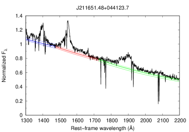
Figure 1: Continuum estimation for J211651.48+044123.7 from our sample. Range 1300 - 1450 Å is shown in blue, 1450 - 1700 Å in red and 1750 - 2200 Å in green. The continuum lines in each range represent from the top: the maximum, the best and the minimum continuum placement.

3.5 Photoionization modeling

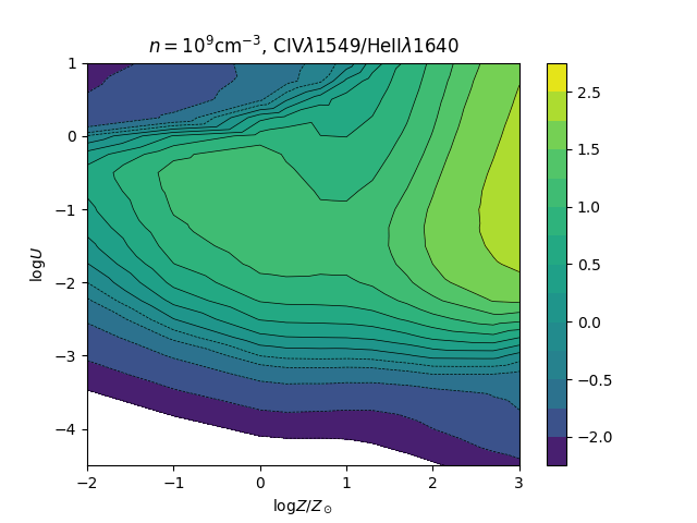
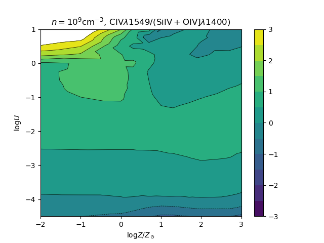
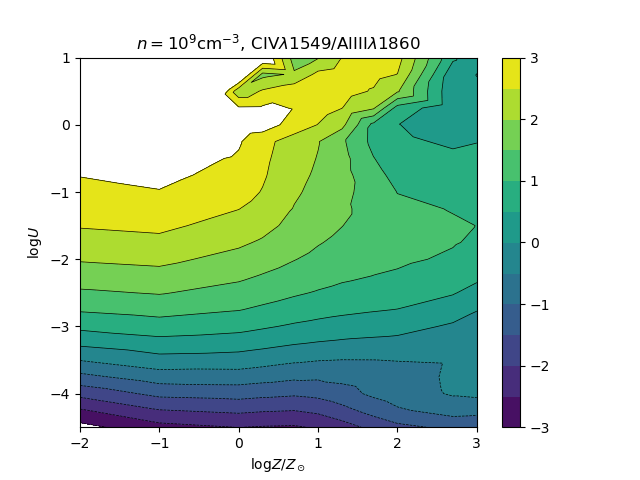
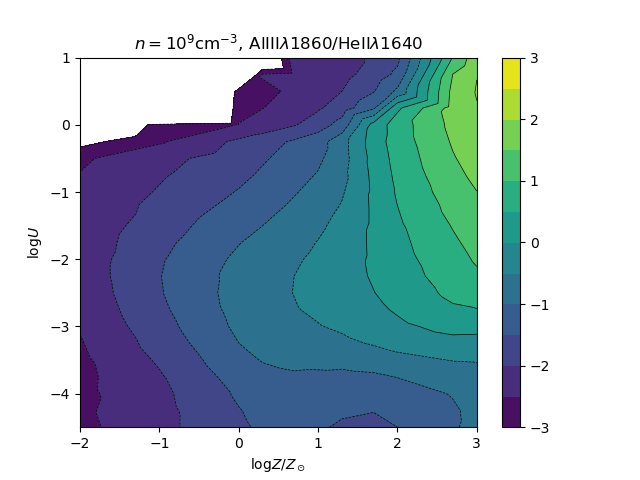
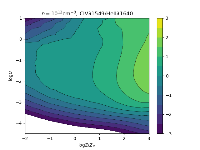
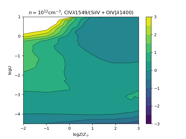
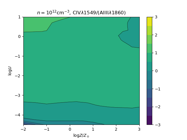
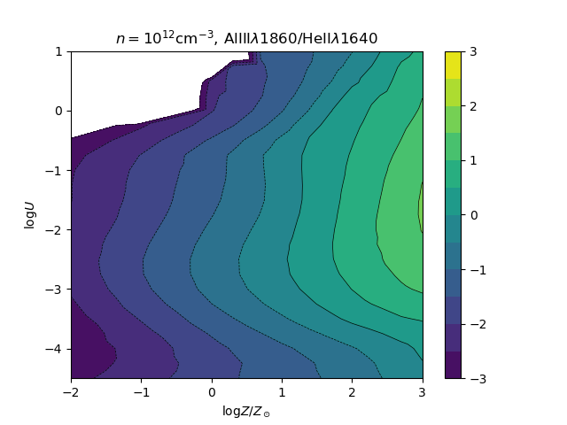
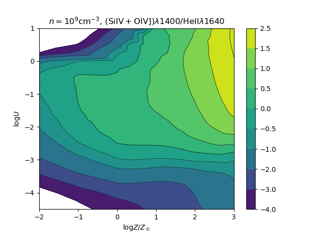
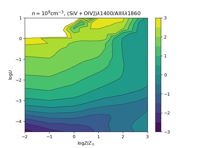
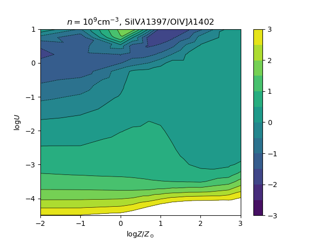
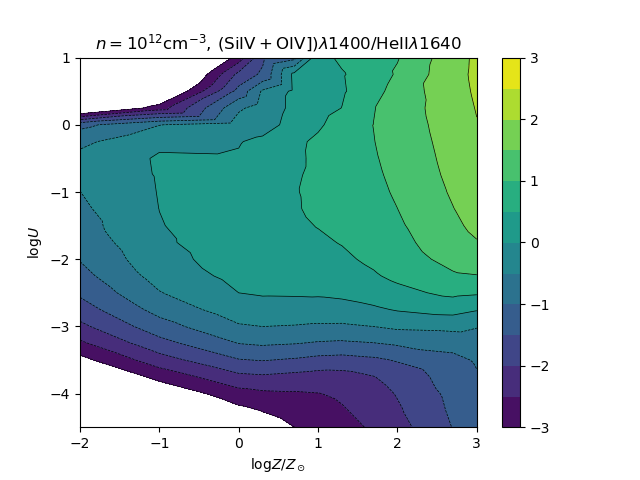
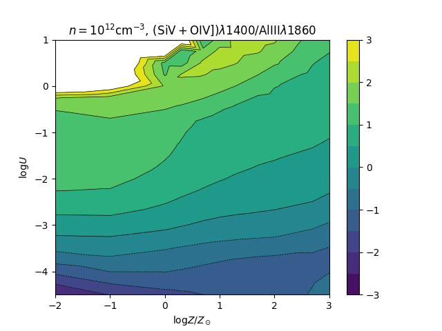
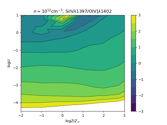
Figure 17: Isophotal contour in the $\log U$ – $\log Z$ plane of seven diagnostic line intensity ratios, computed assuming column density $N_{\mathrm{c}}=10^{23}$ cm^-2. Top rows, from left to right: logarithm of Civ/Heii, Civ/(Siiv+Oiv]), Civ/Aliii, Aliii/Heii$\lambda$1640. Bottom rows, from left to right: logarithm (Siiv+Oiv])/Heii, (Siiv+Oiv])/Aliii, Siiv/Oiv]. The contour plots are shown for $n_{\mathrm{H}}$= $10^{9}$ cm^-3 (top) and $n_{\mathrm{H}}$= $10^{12}$ cm^-3 (bottom) for each diagnostic ratio.

To interpret our fitting results we compare the line intensity ration for BC and BLUE with the ones predicted by CLOUDY 13.05 and 17.02 simulations (Ferland et al., 2013, 2017). An array of simulations is used as reference for comparison with the observed line intensity ratios. It was computed under the assumption that (1) column density is $N_{\mathrm{c}}$ = 10²³ cm^-2; (2) the continuum is represented by the model continuum of Mathews & Ferland (1987) which is believed to be appropriate for Population A quasars, and (3) microturbulence is negligible. The simulation arrays cover the Hydrogen density range 7.00$\leq\log(n_{\mathrm{H}})\leq$14.00 and the ionization parameter $-4.5\leq\log(U)\leq$ 1.00, in intervals of 0.25 dex. They are repeated for values of metallicities in a range encompassing five orders of magnitude: 0.01, 0.1, 1, 2, 5, 10, 20, 50, 100, 200, 500 and 1000 $Z_{\odot}$. Extremely high metallicity $Z\gtrsim 100Z_{\odot}$ is considered physically unrealistic ($Z\approx 100Z_{\odot}$ implies that more than half of the gas mass is made up by metals!), unless the enrichment is provided in situ within the disk (Cantiello et al., 2020). The behavior of diagnostic line ratios as a function of $U$ and $n_{\mathrm{H}}$ for selected values of $Z$ is shown in Fig. 17 of Appendix B.

3.5.1 Basic Interpretation

The line emissivity $\epsilon_{\mathrm{coll}}$ (${\rm ergs\ cm}^{-3}\ {\rm s}^{-1}$) of a collisionally excited line emitted from an element $X$ in its $i-$th ionization stage has a strong temperature dependence. In the high density limit

$$\epsilon_{\mathrm{X^{i},coll}}\ = \ n_{\mathrm{X^{i},l}}\beta A_{\mathrm{X^{i},ul}}h\nu_{\mathrm{0}}\,\frac{g_{\mathrm{X^{i},l}}}{g_{\mathrm{X^{i},u}}}\,\exp{\left(-\frac{h\nu_{0}}{kT_{\mathrm{e}}}\right)}$$

$$\propto n_{\mathrm{X^{i},l}}\exp{\left(-\frac{h\nu_{0}}{kT_{\mathrm{e}}}\right)}$$

the line is said to be “thermalized,” as its strength depends only on the atomic level population and not on the transition strength (Hamann & Ferland, 1999). $\beta$ is the photon escape probability and $A_{\mathrm{X^{i},ul}}$ is the spontaneous decay coefficient. At low densities we have,

$$\epsilon_{\mathrm{X^{i},coll}}\ =\ n_{\mathrm{X^{i},l}}n_{\mathrm{e}}q_{\mathrm{X^{i},lu}}h\nu_{0}\ \propto\ n_{\mathrm{X^{i}}}^{2}T_{\mathrm{e}}^{-1/2}\,\exp{\left(-\frac{h\nu_{0}}{kT_{\mathrm{e}}}\right)}$$ (3)

The recombination lines considered in our analysis are H$\beta$ and Heii$\lambda$1640, for which the emissivity (with an approximate dependence of radiative recombination coefficient $\alpha$ on electron temperature, Osterbrock & Ferland 2006) becomes:

$$\epsilon_{\mathrm{Y^{j},rec}}\ =\ n_{\mathrm{Y^{j}}}\,n_{\mathrm{e}}\,\alpha\,h\nu_{0}\ \propto\ n_{\mathrm{Y^{j}}}^{2}T_{\mathrm{e}}^{-1}\ \ \ \$$ (4)

and $n_{\mathrm{Y^{j}}}$ is the number density of the parent ion.

Under these simplifying, illustrative assumption we can write:

$$\frac{\epsilon_{\mathrm{X^{i},coll}}}{\epsilon_{\mathrm{Y^{j},rec}}}\propto\left(\frac{n_{\mathrm{X^{i}}}}{n_{\mathrm{Y^{j}}}}\right)^{2}T_{\mathrm{e}}^{\frac{1}{2}}\exp{\left(-\frac{h\nu_{0}}{kT_{\mathrm{e}}}\right)}$$ (5)

for the low-density case, and

$$\frac{\epsilon_{\mathrm{X^{i},coll}}}{\epsilon_{\mathrm{Y^{j},rec}}}\propto\frac{n_{\mathrm{X^{i}}}}{n_{\mathrm{Y^{j}}}^{2}}T_{\mathrm{e}}\exp{\left(-\frac{h\nu_{0}}{kT_{\mathrm{e}}}\right)}$$ (6)

for the high density case.

Similarly, for the ratio of two collisionally excited lines at frequencies $\nu_{0}$ and $\nu_{1}$,

$$\frac{\epsilon_{\mathrm{X^{i},coll}}}{\epsilon_{\mathrm{Y^{j},coll}}}\propto\left(\frac{n_{\mathrm{X^{i}}}}{n_{\mathrm{Y^{j}}}}\right)^{\kappa}\exp{\left(-\frac{h(\nu_{0}-\nu_{1})}{kT_{\mathrm{e}}}\right)}$$ (7)

where $\kappa=1,2$ in the high- and low-density case respectively.

Connecting the relative chemical abundance to the line emissivity ratios in the previous equation requires the reconstruction of the ionic stage distribution for each element, i.e., the computation of the ionic equilibrium, as well as the consideration of the extension of the emitting region within the gas clouds i.e., that the line emission is not cospatial, and possible differences in optical depth effects. This is achieved by the CLOUDY simulations. However, we can see that the main variable parameter for a given relative emissivity is $T_{\mathrm{e}}$. In other words, electron temperature is the main parameter connected to metallicity. This is especially true for fixed physical condition ($U$, $n_{\mathrm{H}}$, $N_{\mathrm{c}}=10^{23}$, SED given). This is most likely the case of xA sources: the spectral similarity implies that the scatter in physical properties is modest. We further investigate this issue in Sect. 4.3.

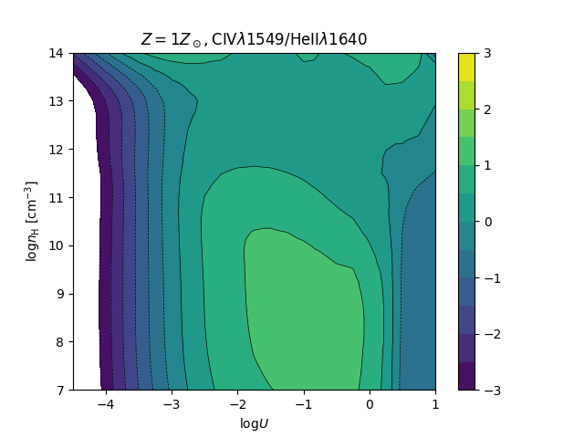
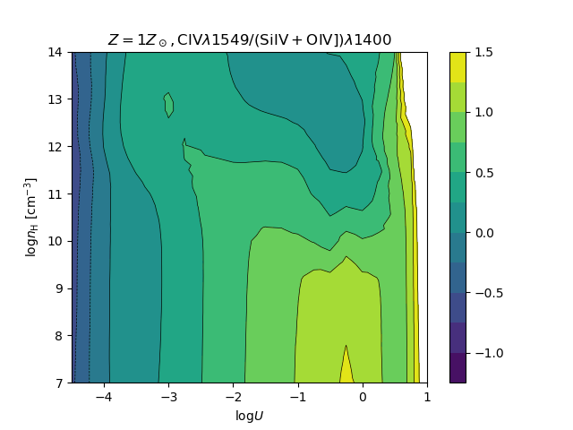
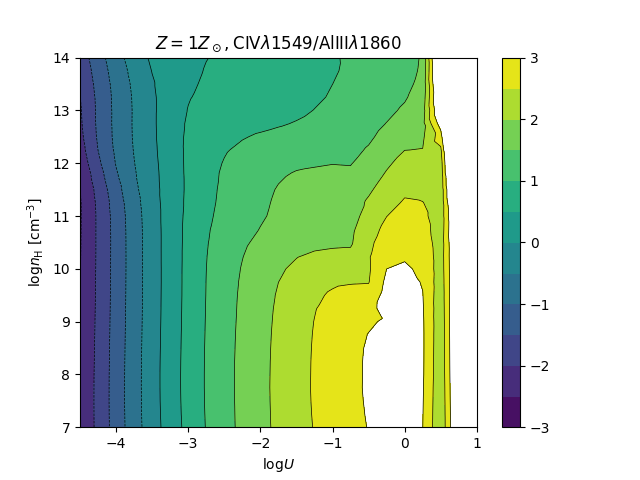
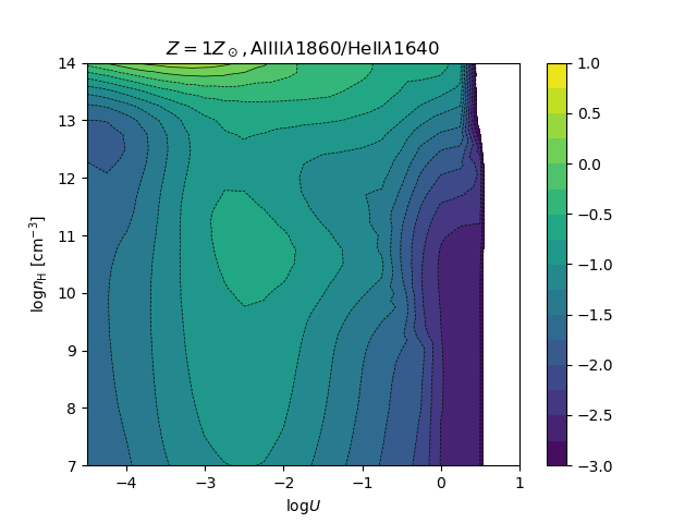
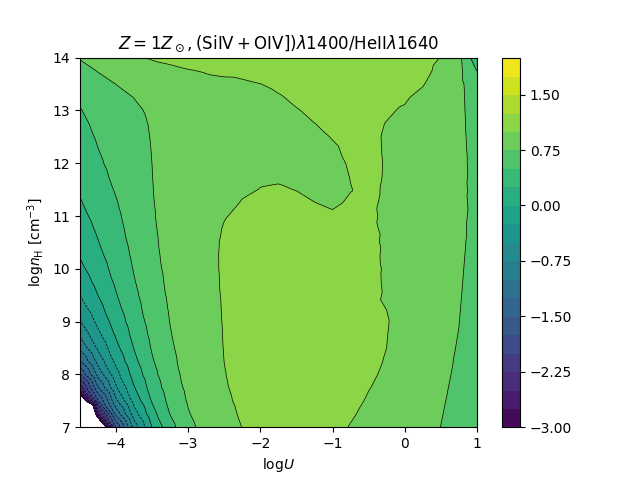
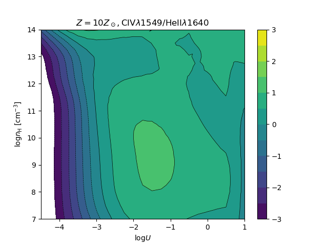
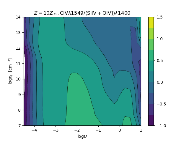
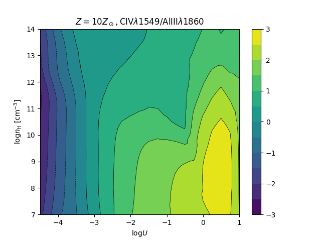
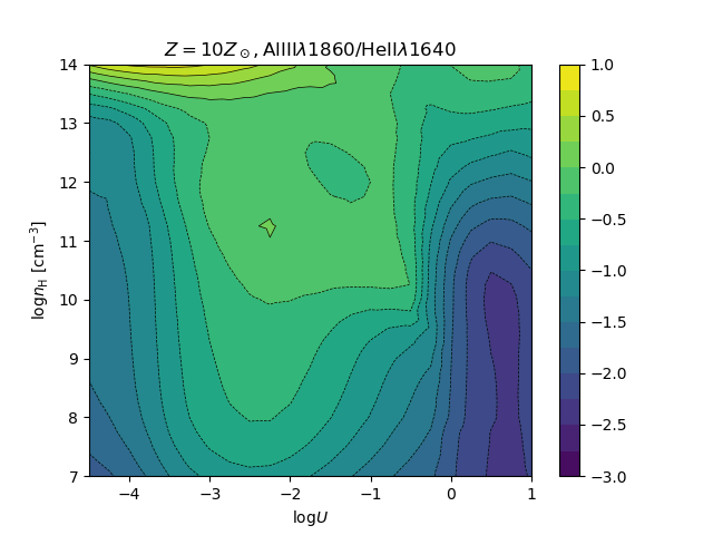
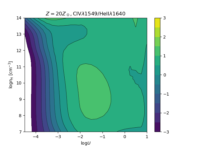
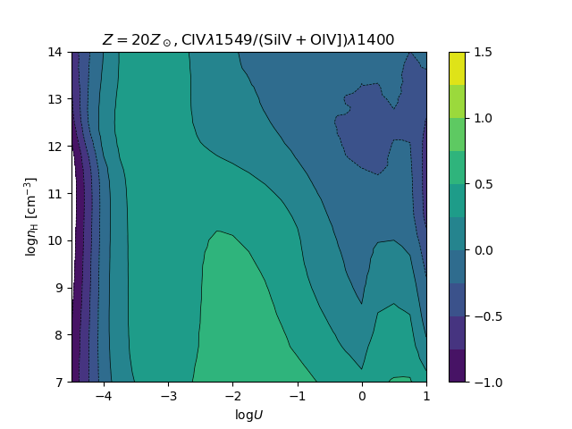
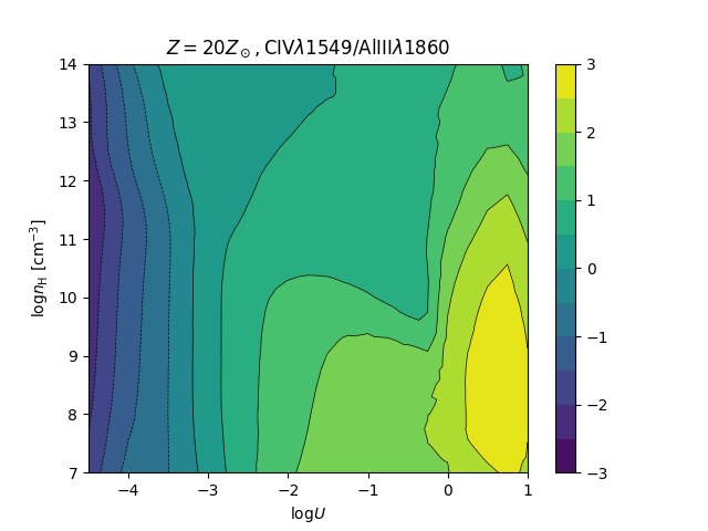
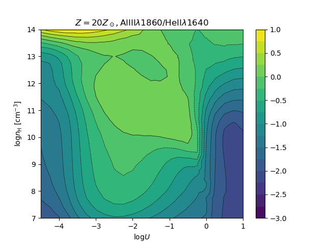
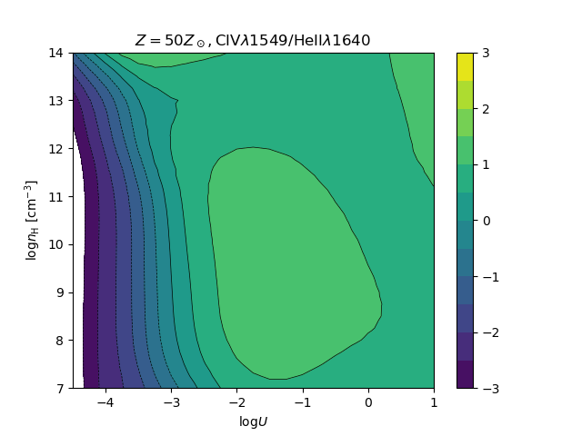
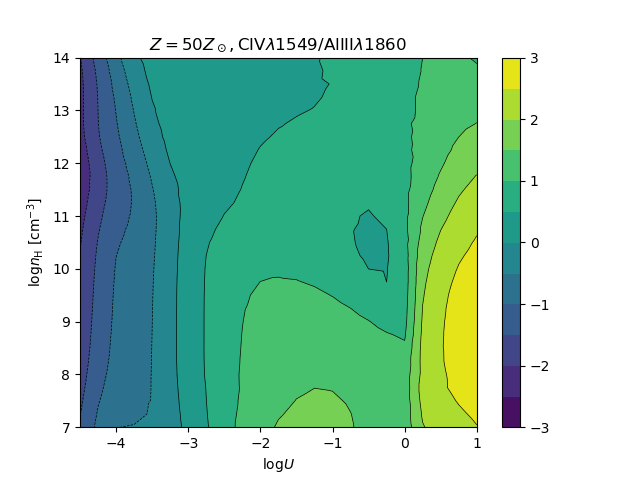
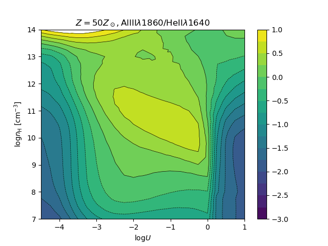
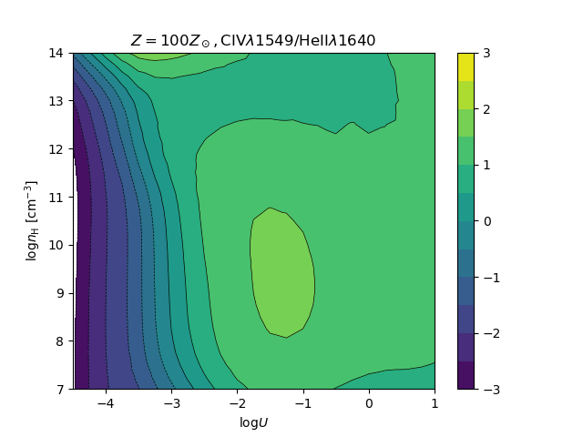
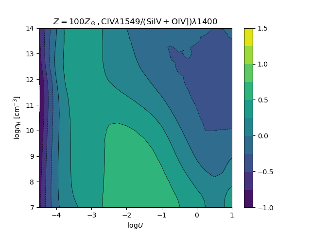
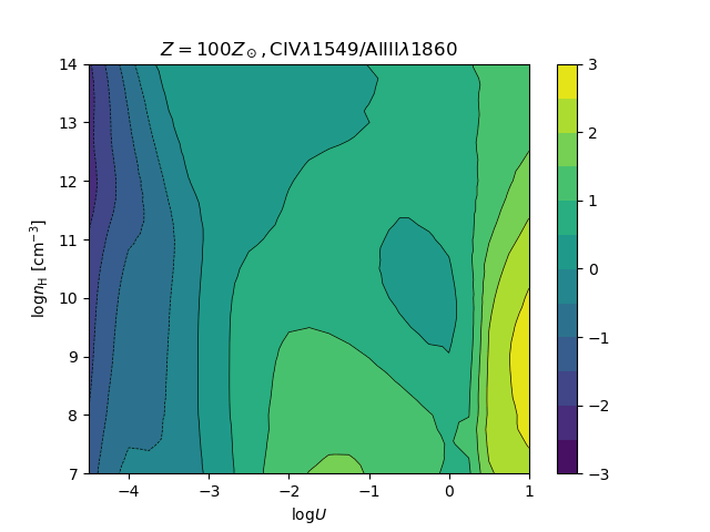
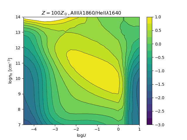
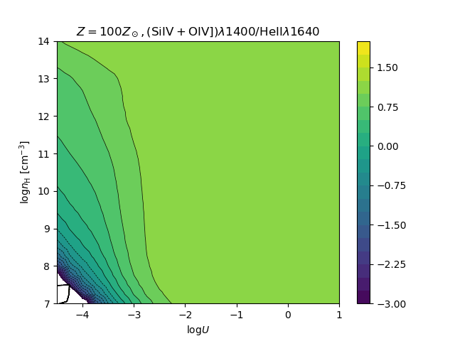
Figure 18: Isophotal contour in the $\log U$ – $\log$ $n_{\mathrm{H}}$ for line intensity ratios (from left to right: Civ/Heii, Civ/(Siiv+Oiv]), Civ/Aliii, Aliii/Heii$\lambda$1640, (Siiv+Oiv])/Heii$\lambda$1640) as a function of metallicity (from top-to-bottom: $Z$ = 1, 10, 20, 50, 100 $Z_{\odot}$), for column density $N_{\mathrm{c}}=10^{23}$ cm^-2.

The electron temperature is also the dominating factor affecting the strength of the Heii$\lambda$1640 line, for a given density. The Heii  Ly$\alpha$ line at 304 Å ionizes Hydrogen atoms and other ionic species with ionization potential up to 3 Ryd. Being absorbed by different ionic species, Heii$\lambda$1640  Ly$\alpha$  cannot sustain a population of excited electrons at the level $n=2$ of Heii$\lambda$1640. This is markedly different from Hydrogen Ly$\alpha$ that in case B is assumed to scatter many times and to sustain a population of Hydrogen atoms at level $n=2$. The Heii line is therefore produced almost only by recombination, and no collisional excitation from level $n=2$ or radiative transfer effects are expected, unlike the case of the Hydrogen Balmer lines (Marziani et al., 2020). The prediction of the Heii line is relatively simple once the electron temperature and the density are known by assumption or computation. The additional advantage in the use of Heii is that there is no significant enhancement of the He abundance over the entire lifetime of the Universe (Peimbert et al., 2001; Peimbert, 2008). The normalization to the Heii line flux of the flux of metal lines should yield robust $Z$ estimates. This is shown by the isophotal contours of Appendix B ( Fig. 17), tracing the behavior of the diagnostic ratios as a function of $Z$ and $U$: the (Siiv+Oiv])/Heii and Aliii/Heii ratios monotonically increase with $Z$ over a large range of $U$; for Civ/Heii$\lambda$1640 the behavior is monotonic at low $U$, but more complex at $\log U\sim-1-0$. Ratios involving pairs of metal lines yield more complex trends in the plane $Z$ – $U$. At low $n_{\mathrm{H}}$, the Civ/Aliii ratio is a good $Z$ estimator, although of limited usefulness since Aliii is weak; at high $n_{\mathrm{H}}$, its sensitivity is greatly reduced (Appendix B; Fig. 17). The Civ/(Siiv+ Oiv]) does not appear to be especially sensitive to $Z$. The diagnostic ratios change as a function of $Z$, although the behavior as a function of $n_{\mathrm{H}}$ and $U$ is roughly preserved (Appendix B; Fig. 18).

3.6 Explorative analysis of photoionization trends at fixed ionization parameter and density

One of the main results of previous investigations is the systematic differences in ionization between BLUE and BC (Marziani et al., 2010; Negrete et al., 2012; Sulentic et al., 2017). Previous inferences suggest very low ionization ($U\sim 10^{-2.5}$), also because of the relatively low Civ/H$\beta$ ratio for the BC emitting part of the BLR, and high density. A robust lower limit to density $n_{\mathrm{H}}$$\sim 10^{11.5}$ cm^-3  has been obtained from the analysis of the CaII triplet emission (Matsuoka et al., 2007; Panda et al., 2020a). Less constrained are the physical conditions for BLUE emission. Apart from Civ/H$\beta$$\gg 1$ and Ly$\alpha$/H$\beta$ and Civ/Ciii] also $\gg 1$, little constraints exist on density and column density. This result hardly comes as a surprise considering the difference in dynamical status associated with the two components. While it is expected that the BC is emitted in a region of high column density $\log$$N_{\rm c}$$\gtrsim 23$ [cm^-2], not last because radiation forces are proportional to the inverse of $N_{\mathrm{c}}$ (Netzer & Marziani, 2010, see also Ferland et al. 2009). More explicitly, the equation of motion for a gas cloud under the combined effect of gravitation and radiation forces contains an acceleration term due to radiation that is inversely proportional to $N_{\mathrm{c}}$. The high $N_{\rm c}$ region is expected to be relatively stable (at rest frame, with no sign of systematic, large shifts in Population A) and presumably devoid of low-density gas (considering the weakness of Ciii], Negrete et al. 2012). The same cannot be assumed for BLUE. BLUE is associated with a high radial velocity outflow, probably with the outflowing streams creating BAL features when intercepted by the line-of-sight (e.g., Elvis, 2000).

Here we consider $\log U=-2.5$, $\log$ $n_{\mathrm{H}}$=12 (-2.5,12), and $\log U=0,\log$$n_{\mathrm{H}}$=9 (0,9) as representative of the low and high- ionization emitting gas. Fig. 2 illustrates the behavior of the Civ/H$\beta$, Heii$\lambda$1640/H$\beta$ and Civ/Heii$\lambda$1640 in the high and low-ionization cases as a function of metallicity. The Civ intensity with respect to H$\beta$ has a steep drop around $Z\gtrsim 1Z_{\odot}$, after a steady increase for sub-solar $Z$. The Heii$\lambda$1640/H$\beta$ ratio decreases steadily, with a steepening at round solar value. Physically, this behavior is due to the high value of the ionization parameter (assumed constant), while the electron temperature decreases with metallicity, implying a much lower collisional excitation rate for Civ production. The dominant effect for the Heii$\lambda$1640 decrease is likely the “ionization competition” between Civ and Heii$\lambda$1640 parent ionic species (Hamann & Ferland, 1999). As a consequence, the ratio Civ/Heii$\lambda$1640 has a non-monotonic behavior with a local maximum around solar metallicity. At low ionization and high density, the behavior is more regular, as the steady increase in Civ/H$\beta$ is followed by a saturation to a maximum Civ/H$\beta$. The Heii$\lambda$1640/H$\beta$ ratio is constant up to solar, and steadily decreases above solar, where the ionization competition with triply-ionized carbon sets on. The result is a smooth, steady increase in the Civ/Heii$\lambda$1640 ratio.

Fig. 3 shows the behavior of the other intensity ratios used as metallicity diagnostics, for BLUE and BC. Siiv+Oiv]/Civ and Siiv+Oiv]/Heii$\lambda$1640 saturate above 100 $Z_{\odot}$. Only around $Z\sim 10Z_{\odot}$ values Civ/Siiv+Oiv]$\lesssim$ 1 are possible, but the behavior is not monotonic and the ratio rises again at $Z\gtrsim 30Z_{\odot}$, with the unpleasant consequence that a ratio Civ/Siiv+Oiv]$\approx 1.6$ might imply 10 $Z_{\odot}$ as well as 1000 $Z_{\odot}$. The ratios usable for the BC also show regular behavior. The Civ/Aliii ratio remains almost constant up $Z\sim 0.1Z_{\odot}$, and the starts a regular decrease with increasing $Z$, due to the decrease of $T_{\mathrm{e}}$ with $Z$ (Civ is affected more strongly than Aliii). Interestingly, Aliii/Heii$\lambda$1640 shows the opposite trend, due to the steady decrease of the Heii$\lambda$1640 prominence with $Z$. Especially of interest is however the behavior of ratio Aliii/Heii$\lambda$1640 that shows a monotonic, very linear behavior in the log-log diagram. As for the high-ionization case, values (Siiv+Oiv])/Civ$\gtrsim$ 1 are possible only at very high metallicity, although the non monotonic behavior (around the minimum at $Z\approx 200Z_{\odot}$) complicates the interpretation of the observed emission line ratios.

Figure 2: Computed intensity ratios involving Civ and Heii$\lambda$1640 as a function of metallicity, for physical parameters $U$ and $n_{\mathrm{H}}$ fixed: ($\log U$, $\log$ $n_{\mathrm{H}}$) = (-1,9) (top) and ($\log U$, $\log$ $n_{\mathrm{H}}$) = (-2.5,12) (bottom). Columns from left to right show Civ/H$\beta$, Heii$\lambda$1640/H$\beta$, Civ/Heii$\lambda$1640.

Figure 3: Behavior of the intensity ratios employed in this work (with the exception of Civ/Heii$\lambda$1640 shown in the previous Figure), as a function of metallicity, for physical parameters $U$ and $n_{\mathrm{H}}$ fixed: ($\log U$, $\log$ $n_{\mathrm{H}}$) = (-1,9) and ($\log U$, $\log$ $n_{\mathrm{H}}$) = (-2.5,12). Top panels, from left to right: Civ/Siiv+Oiv],(Siiv+Oiv])/Heii$\lambda$1640, Civ/Aliii. Bottom panes, from left to right: Aliii/Heii$\lambda$1640, Civ/(Siiv+Oiv]), (Siiv+Oiv])/Heii$\lambda$1640.

The ionization structure within the slab remains self similar over a wide metallicity range, with the same systematic differences between the high and low-ionization case (Fig. 4), consistent with the assumption of a constant ionization parameter. As expected, the electron temperature decreases with metallicity, and the transition between the fully and partially ionized zone (FIZ and PIZ) occurs at smaller depth. In addition, close to the illuminated side of the cloud the electron temperature remains almost constant; the gas starts becoming colder before the transition from FIZ to PIZ. The depth at which $T_{\mathrm{e}}$ starts decreasing is well-defined, and its value becomes lower with increasing $Z$  (Fig. 4). The effect is present for both the low- and high- ionization case, although it is more pronounced for the high-ionization. Fig. 5 shows how an increase in metallicity is affecting the $T_{\mathrm{e}}$  in the line emitting cloud. Fig. 5 reports the behavior of $T_{\mathrm{e}}$ at the illuminated face of the cloud ($\tau\sim 0$) and at maximum $\tau$ (corresponding to $N_{\rm c}$= 10²³ cm^-2, the side facing the observer) for the high-ionization and low-ionization case. The $T_{\mathrm{e}}$  monotonically decreases as a function of metallicity. The difference between the two cloud faces is almost constant for the low ionization case, with $\delta\log T_{\mathrm{e}}\approx 0.5$ dex, while it increases for the high-ionization case, reaching $\delta\log T_{\mathrm{e}}\approx 0.75$ dex at the highet $Z$ value considered, 10${}^{3}Z_{\odot}$.

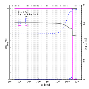
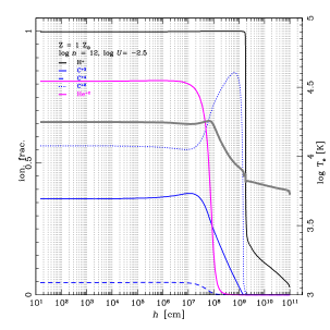
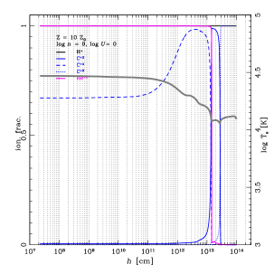
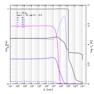
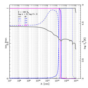
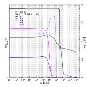
Figure 4: Ionization fraction and electron temperature (thick grey line) as a function of depth within the emitting gas slab, for physical parameters $U$ and $n_{\mathrm{H}}$ fixed, computed with CLOUDY 13.05: ($\log U$, $\log$ $n_{\mathrm{H}}$) = (-1,9) (representative of BLUE and high ionization case, left) and ($\log U$, $\log$ $n_{\mathrm{H}}$) = (-2.5,12) (representative of the low-ionization BLR, right), in order of increasing metallicity from top to bottom.

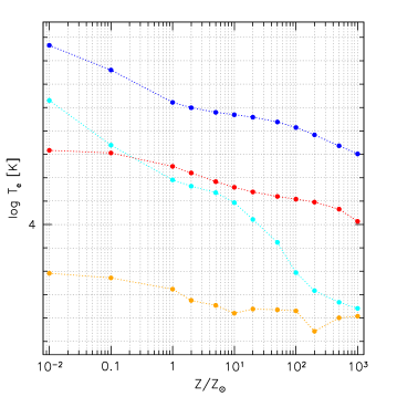
Figure 5: Electron temperature $T_{\mathrm{e}}$ as a function of metallicity $Z$, for physical parameters $U$ and $n_{\mathrm{H}}$ fixed: ($\log U$, $\log$ $n_{\mathrm{H}}$) = (-1,9) (representative of BLUE and high ionization case, blue and cyan) and ($\log U$, $\log$ $n_{\mathrm{H}}$) = (-2.5,12) (representative of the low-ionization BLR, red and orange), from CLOUDY 13.05 computations. Blue and red refer to the first zone of the CLOUDY computation i.e., to the illuminated surface of the clouds; cyan and orange, to the side of the cloud farther from the continuum sources i.e., facing the observer.

4 Results

4.1 Immediate Results

The observational results of our analysis involve the measurements of the intensity of the line BC and BLUE component separately. The rest-frame spectra with the continuum placements, and the fits to the blends of the spectra are shown in Appendix A. Table 2 reports the measurement for the $\lambda$1900 blend. The columns list the SDSS identification code, the FWHM (in units of km s^-1) and equivalent width and flux of Aliii (the sum of the doublet lines, in units of Å and 10^-14 erg s^-1 cm^-2, respectively), FWHM and flux of Ciii], and flux of Siiii] (its FWHM is assumed equal to the one of the single Aliii lines.) with Similarly, Table 3 reports the parameter of the Civ blend: equivalent width, FWHM and flux of the Civ BC, the flux of the Civ blueshifted component, as well as the fluxes of the BC and BLUE of Heii$\lambda$1640. FWHM values are reported but especially values $\gtrsim 5000$ km s^-1 should be considered as highly uncertain. There is the concrete possibility of an additional broadening ($\sim$ 10 % of the observed FWHM) associated with non-virial motions for the Aliii line (del Olmo et al., in preparation). The fluxes of the BC and of BLUE of Siiv and Oiv] are reported in Table 4. Intensity ratios with uncertainties are reported in Table 5. The last row lists the median values of the ratios with their semi-interquartile ranges (SIQR).

4.1.1 Identification of xA sources and of “intruders”

Figure 6 shows that the majority of sources meet both UV selection criteria, and should be considered xA quasars. The median value of the Aliii/Siiii] (last row of Table 5) implies that the Aliii is strong relative to Siiii]. Also Siiii] is stronger than Ciii]. Both selection criteria are satisfied by the median ratios. Only one source (SDSS J084525.84+072222.3 (catalog )) shows Ciii]/Siiii] significantly larger than 1. This quasar is however confirmed as an xA by the very large Aliii/Siiii], by the blueshift of Civ, and by the prominent $\lambda$1400 blend comparable to the Civ emission. The lines in the spectrum of SDSS J084525.84+072222.3 (catalog ) are broad, and any Ciii] emission is heavily blended with Feiii emission. The Ciii] value should be considered an upper limit. Three outlying/borderline data points (in orange) in Fig. 6 have ratio Ciii]/Siiii]$\sim 1$, and Aliii/Siiii] consistent with the selection criteria within the uncertainties, but other criteria support their classification as xA. The borderline sources will be further discussed in Section 4.3. In conclusion, all the 13 sources of the present sample save one should be considered bona-fide xA sources.

It is intriguing that the intensity ratios Ciii]/Siiii] and Aliii/Siiii] are apparently anti-correlated in Figure 6, if we exclude the two outlying points. Excluding the two outlying data point the Spearman rank correlation coefficient is $\rho\approx 0.8$, which implies a $4\sigma$ significance for a correlation, but the correlation coefficient between the two ratios for the full sample is much lower. Given the small number of sources, a larger sample is needed to confirm the trend.

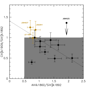
Figure 6: Relation between intensity ratios AlIII$\lambda$1860/SiIII]$\lambda$1892 and CIII]$\lambda$1909/SiIII]$\lambda$1892. The gray area corresponds to the parameter space occupied by the xA sources. Borderline sources are in orange color.

4.1.2 BC intensity ratios

Fig. 7 shows the distributon of diagnostic intensity ratios Civ/Heii$\lambda$1640, Siiv/Heii$\lambda$1640, and Aliii/Heii$\lambda$1640 for the BC. The lower panels of Fig. 7 shows the results for individual sources.

The vertical lines identify the median values, $\mu_{\frac{1}{2}}$(Civ/Heii$\lambda$1640)$\approx 4.03$, $\mu_{\frac{1}{2}}$(Aliii/Heii$\lambda$1640)$\approx$ 4.31, $\mu_{\frac{1}{2}}$(Siiv/Heii$\lambda$1640) $\approx$ 6.39. The higher value for Siiv/Heii$\lambda$1640 than for Civ/Heii$\lambda$1640 implies $\mu_{\frac{1}{2}}$(Civ/Siiv) $\approx$ 0.69, a value that is predicted by CLOUDY for very low values of the ionization parameter (Appendix B). The Civ/Aliii ratio is also constraining: the CLOUDY simulations indicate high $Z$ and low ionization.

The distribution of the data points is relatively well-behaved, with individual ratios showing small scatter around their median values. In the histogram, we see a tail made by a 3-5 objects suggesting systematically higher values. In particular, at least two objects (SDSS J102606.67+011459.0 (catalog ) and SDSS J085856.00+015219.4 (catalog )) show systematically higher ratios, with Civ/Heii$\lambda$1640$\approx 10$, and Aliii/Heii$\lambda$1640$\approx 4$. Both of them show extreme Civ blueshifts and SDSS J102606.67+011459.0 (catalog ) shows the highest Aliii/Siiii] ratio in the sample.

Since the three ratios are, for fixed physical conditions, proportional to metallicity, we expect an overall consistency in their behavior i.e., if one ratio is higher than the median for one object, also the other intensity ratios should be also higher. The lower diagrams are helpful to identify sources for which only one intensity ratio deviates significantly from the rest of the sample. A case in point is SDSS J082936.30+080140.6 (catalog ) whose ratio Aliii/Heii$\lambda$1640$\approx 8$ is one of the highest values, but whose Civ/Heii$\lambda$1640 and Siiv/Heii$\lambda$1640 are slightly below the median values. The fits of Appendix A show that this object is indeed extreme in Aliii emission. The Civ and $\lambda$1400 blends are dominated by the BLUE excess, and an estimate of the Civ and Siiv BC is very difficult, as it accounts for a small fraction of the line emission. The Heii$\lambda$1640 emission is almost undetectable, especially in correspondence to the rest frame. SDSS J082936.30+080140.6 (catalog ), along with other sources with high Aliii/Heii$\lambda$1640 or Siiv/Heii$\lambda$1640 ratios may indicate selective enhancement of Aluminium or Silicon (see also Sect. 5.7).

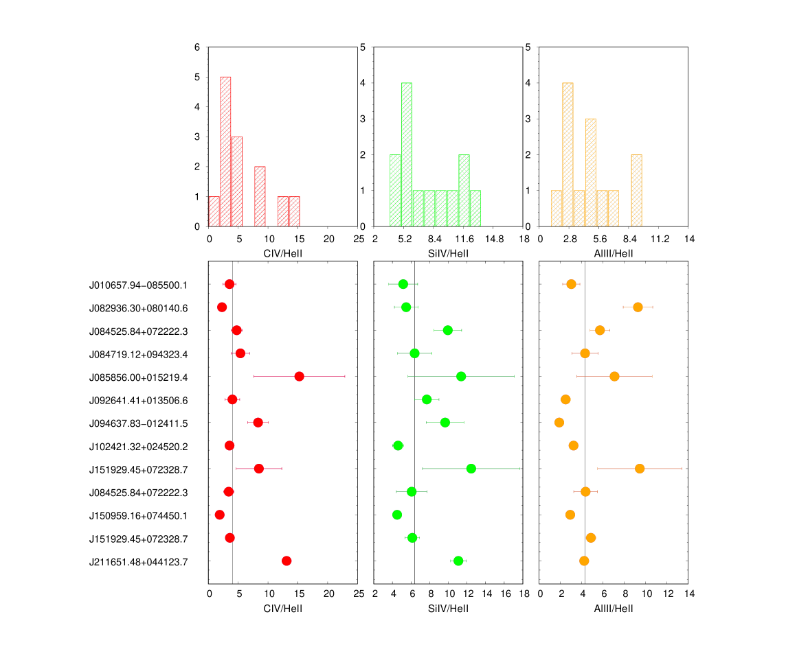
Figure 7: Distribution of diagnostic intensity ratios based on the BC (top) for Civ/Heii$\lambda$1640 (red), Siiv/Heii$\lambda$1640 (green) and Aliii/Heii$\lambda$1640 (orange). The lower panels show results and associated uncertainties for individual sources with the same color-coding as histograms. Vertical black line in lower panel represents median value of sources measurements.

4.1.3 BLUE intensity ratios

Similar considerations apply to the blue intensity ratios. We see systematic trends in Figure 8 that imply consistency of the ratios for most sources, although the uncertainties are larger, especially for Civ/Heii$\lambda$1640. The ratio Civ/(Siiv+ Oiv]) values are systematically higher than for the BC, while the Civ/Heii$\lambda$1640 is slightly higher (median BLUE 5.8 vs. median BC 4.38). The ratio (Siiv+ Oiv])/Heii$\lambda$1640 is much lower than for the BC (median BLUE 2.09 vs. median BC 6.27). The difference might be in part explained by the difficulty of deblending Siiv from Oiv], and by the frequent occurrence of absorptions affecting the blue side of the blend. Both factors may conspire to depress BLUE. The lower diagrams of Fig. 8 are again helpful to identify sources for which intensity ratios deviate significantly from the rest of the sample. SDSS J102606.67+011459.0 (catalog ) shows a strong enhancement of Civ/Heii$\lambda$1640 and Siiv+Oiv], confirming the trend seen in its BC.

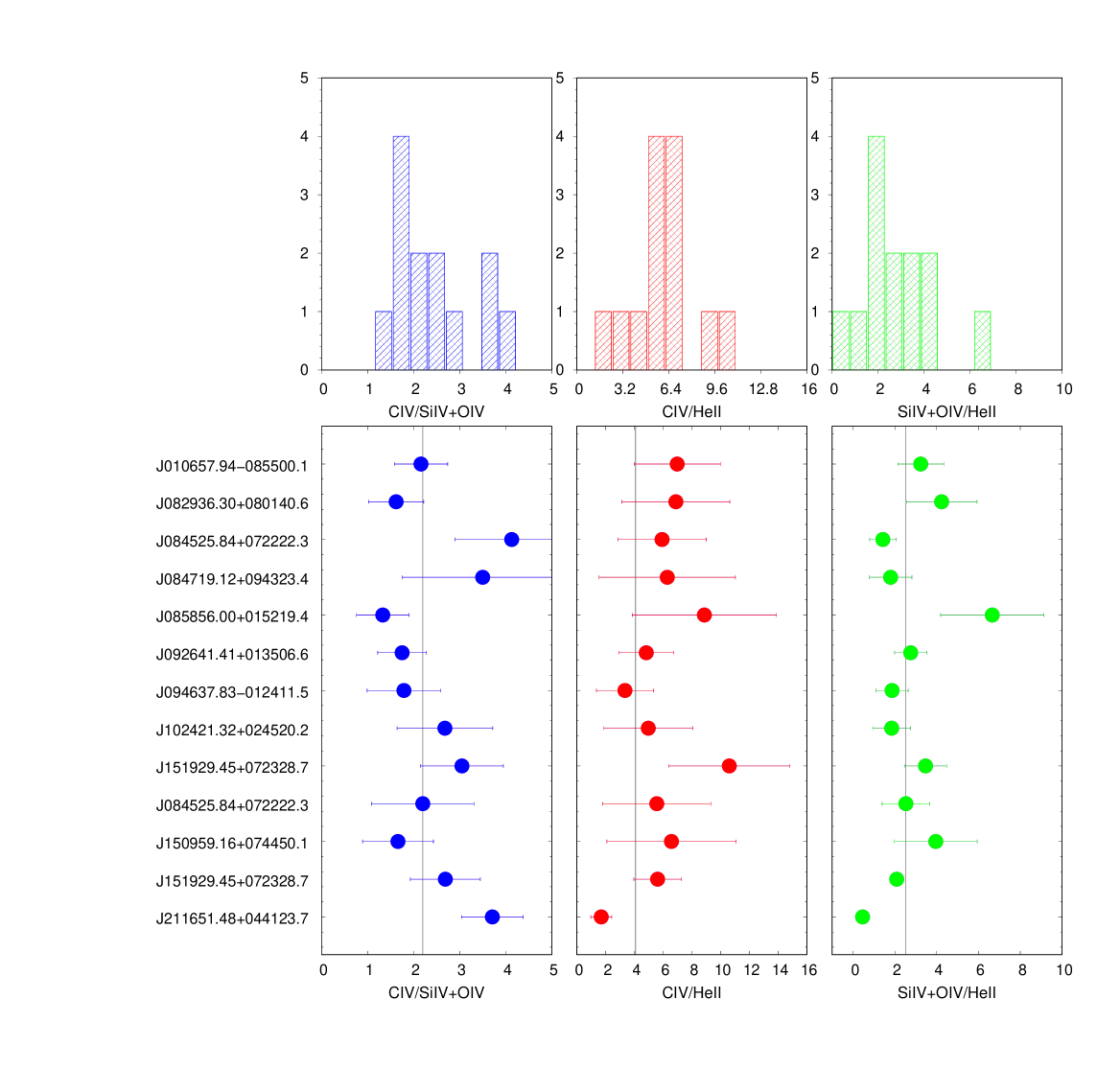
Figure 8: Distribution of diagnostic intensity ratios based on the BLUE components (top) for Civ/Siiv+Oiv] (blue), Civ/Heii$\lambda$1640 (red) and Siiv+Oiv]/Heii$\lambda$1640 (green). The lower panels show results and associated uncertainties for individual sources with the same color-coding as histograms, as in the previous Figure. Vertical black line represents median value of ratios measurements.

Table 2: Measurements in the 1900Å blend region.

SDSS JCODE	Aliii	Aliii	Aliii	Ciii]	Ciii]	Siiii]
	$W$	FWHM	Flux	FWHM	Flux	Flux
(1)	(2)	(3)	(4)	(5)	(6)	(7)
J010657.94-085500.1	7.9	5560	5.41 $\pm$ 0.38	6050	2.88 $\pm$ 0.14	7.2 $\pm$ 0.93
J082936.30+080140.6	10.2	5710	7.43 $\pm$ 0.42	5950	2.39 $\pm$ 0.21	4.85 $\pm$ 0.66
J084525.84+072222.3	13.1	5510	6.04 $\pm$ 0.52	5570	4.25 $\pm$ 0.53	3.13 $\pm$ 0.08
J084719.12+094323.4	9.9	5410	9.24 $\pm$ 0.24	5630	4.63 $\pm$ 0.36	5.61 $\pm$ 0.73
J085856.00+015219.4	7.7	5520	4.57 $\pm$ 0.37	5660	3.98 $\pm$ 0.12	4.39 $\pm$ 0.58
J092641.41+013506.6	8.0	5550	4.82 $\pm$ 0.3	5720	6.53 $\pm$ 0.23	5.48 $\pm$ 0.96
J094637.83-012411.5	5.0	2730	3.54 $\pm$ 0.24	2090	6.38 $\pm$ 0.22	5.1 $\pm$ 0.67
J102421.32+024520.2	10.1	5520	6.15 $\pm$ 0.31	6080	3.31 $\pm$ 0.2	5.1 $\pm$ 0.39
J102606.67+011459.0	9.5	5590	7.7 $\pm$ 0.35	5470	1.83 $\pm$ 0.33	3.64 $\pm$ 0.3
J114557.84+080029.0	11.4	5520	8.74 $\pm$ 0.38	6060	5.91 $\pm$ 0.83	6.3 $\pm$ 0.81
J150959.16+074450.1	11.8	5530	6.44 $\pm$ 0.53	6090	7.62 $\pm$ 0.25	7.58 $\pm$ 1.32
J151929.45+072328.7	10.5	5320	7.37 $\pm$ 0.51	5310	5.6 $\pm$ 0.62	7.16 $\pm$ 1.12
J211651.48+044123.7	6.1	5550	4.21 $\pm$ 0.4	5620	5.29 $\pm$ 0.2	5.35 $\pm$ 0.7

Note. — Columns are as follows: (1) SDSS name, (2) and (3) report the FWHM of Aliii and Ciii] in km s^-1; (4), (5) and (6) list the fluxes in units of 10^-14 erg s^-1cm^-2 for Aliii, Ciii], and Siiii].

Table 3: Measurements in the Civ spectral region

SDSS JCODE	Civ	Civ BC	Civ BC	Civ BLUE	Heii BC	Heii BLUE
	W	FWHM	Flux	Flux	Flux	Flux
(1)	(2)	(3)	(4)	(5)	(6)	(7)
J010657.94-085500.1	18.6	5530	6.35 $\pm$ 1.04	13.46 $\pm$ 0.13	1.79 $\pm$ 0.46	1.93 $\pm$ 0.65
J082936.30+080140.6	15.5	3710 $\pm$ 670	1.83 $\pm$ 0.4	11.86 $\pm$ 0.03	0.8 $\pm$ 0.11	1.72 $\pm$ 0.69
J084525.84+072222.3	16.8	3760	5.04 $\pm$ 0.68	11.11 $\pm$ 0.21	1.06 $\pm$ 0.15	1.87 $\pm$ 0.81
J084719.12+094323.4	17.6	5520	11.53 $\pm$ 0.53	13.24 $\pm$ 0.07	2.14 $\pm$ 0.61	2.1 $\pm$ 1.19
J085856.00+015219.4	22.8	5460	9.84 $\pm$ 0.82	11.39 $\pm$ 0.09	0.65 $\pm$ 0.32	1.28 $\pm$ 0.48
J092641.41+013506.6	25.5	5550	7.79 $\pm$ 1.98	7.08 $\pm$ 0.08	1.94 $\pm$ 0.33	1.47 $\pm$ 0.39
J094637.83-012411.5	23.6	3670	15.63 $\pm$ 0.6	5.89 $\pm$ 0.09	1.87 $\pm$ 0.39	1.76 $\pm$ 0.7
J102421.32+024520.2	20.1	5640	6.74 $\pm$ 0.45	10.9 $\pm$ 0.08	1.9 $\pm$ 0.19	2.19 $\pm$ 1.07
J102606.67+011459.0	17.3	3700 $\pm$ 650	6.92 $\pm$ 1.22	12.23 $\pm$ 0.05	0.82 $\pm$ 0.34	1.15 $\pm$ 0.32
J114557.84+080029.0	18.4	3500 $\pm$ 700	6.84 $\pm$ 0.3	12.57 $\pm$ 0.03	2.01 $\pm$ 0.5	2.26 $\pm$ 1.02
J150959.16+074450.1	16.8	3530 $\pm$ 690	4.19 $\pm$ 0.84	9.73 $\pm$ 0.22	2.21 $\pm$ 0.14	1.48 $\pm$ 0.74
J151929.45+072328.7	19.4	3470 $\pm$ 590	5.47 $\pm$ 0.41	12.04 $\pm$ 0.16	1.52 $\pm$ 0.09	2.14 $\pm$ 0.24
J211651.48+044123.7	19.1	4750	13.04 $\pm$ 0.68	3.01 $\pm$ 0.24	0.99 $\pm$ 0.03	1.77 $\pm$ 0.69

Note. Columns are as follows: (1) SDSS name, (2) rest-frame equivalent width of the total Civ emission i.e., Civ BLUE+BC, in Å; (3) the FWHM of the Civ line in km s^-1; Cols. (4) and (5) list fluxes of the Civ BC and BLUE line; Cols. (6) and (7) report fluxes of the BC and BLUE components for the Heii$\lambda$1640 line. All fluxed are in units of 10^-14 erg s^-1cm^-2.

Table 4: Measurements in the $\lambda 1400$ region.

SDSS JCODE	Siiv+Oiv] BC	Siiv+Oiv] BC	Siiv+Oiv] BLUE
	FWHM	Flux	Flux
(1)	(2)	(3)	(4)
J010657.94-085500.1	5070	9.23 $\pm$ 1.4	6.24 $\pm$ 0.24
J082936.30+080140.6	5560	4.39 $\pm$ 0.81	7.3 $\pm$ 0.06
J084525.84+072222.3	5060	10.52 $\pm$ 0.58	2.69 $\pm$ 0.24
J084719.12+094323.4	5550	13.69 $\pm$ 0.86	3.79 $\pm$ 0.19
J085856.00+015219.4	6960	7.34 $\pm$ 0.69	8.55 $\pm$ 0.05
J092641.41+013506.6	5540	14.89 $\pm$ 0.45	4.05 $\pm$ 0.32
J094637.83-012411.5	4030	18.09 $\pm$ 0.7	3.29 $\pm$ 0.31
J102421.32+024520.2	5530	8.77 $\pm$ 0.64	4.06 $\pm$ 0.09
J102606.67+011459.0	5300	10.16 $\pm$ 0.57	4.01 $\pm$ 0.33
J114557.84+080029.0	3760	12.19 $\pm$ 1.22	5.71 $\pm$ 0.08
J150959.16+074450.1	3650	9.97 $\pm$ 0.75	5.86 $\pm$ 0.12
J151929.45+072328.7	3670	9.32 $\pm$ 1.05	4.48 $\pm$ 0.31
J211651.48+044123.7	4770	11.02 $\pm$ 0.77	0.81 $\pm$ 0.03

Note. Columns are as follows: (1) SDSS name, (2) the FWHM of the Siiv line in km s^-1. (3) and (4) list fluxes of the broad components and the blue component line in units of 10^-14 ergs^-1cm^-2.

Table 5: Intensity ratios for the BC and BLUE line components

SDSS JCODE	Aliii/Siiii]	Ciii]/Siiii]	Civ/Siiv	Civ/Heii$\lambda$1640	Siiv/Heii$\lambda$1640	Civ/Aliii	Aliii/Heii$\lambda$1640	Civ/Heii$\lambda$1640	Civ/Siiv+ Oiv]	Siiv+ Oiv]/ Heii$\lambda$1640
	(BC)	(BC)	(BC)	(BC)	(BC)	(BC)	(BC)	(BLUE)	(BLUE)	(BLUE)
(1)	(2)	(3)	(4)	(5)	(6)	(7)	(8)	(9)	(10)	(11)
J010657.94-085500.1	0.75 $\pm$ 0.11	0.4 $\pm$ 0.05	0.69 $\pm$ 0.15	3.55 $\pm$ 1.09	5.16 $\pm$ 1.55	1.17 $\pm$ 0.21	3.02 $\pm$ 0.81	6.98 $\pm$ 3	2.16 $\pm$ 0.58	3.24 $\pm$ 1.1
J082936.30+080140.6	1.53 $\pm$ 0.23	0.49 $\pm$ 0.08	0.42 $\pm$ 0.12	2.29 $\pm$ 0.6	5.48 $\pm$ 1.26	0.25 $\pm$ 0.06	9.28 $\pm$ 1.39	6.89 $\pm$ 3.75	1.62 $\pm$ 0.6	4.24 $\pm$ 1.69
J084525.84+072222.3	1.93 $\pm$ 0.17	1.36 $\pm$ 0.17	0.48 $\pm$ 0.07	4.76 $\pm$ 0.92	9.95 $\pm$ 1.48	0.83 $\pm$ 0.13	5.71 $\pm$ 0.93	5.93 $\pm$ 3.07	4.13 $\pm$ 1.23	1.43 $\pm$ 0.63
J084719.12+094323.4	1.65 $\pm$ 0.22	0.82 $\pm$ 0.12	0.84 $\pm$ 0.07	5.38 $\pm$ 1.55	6.39 $\pm$ 1.86	1.25 $\pm$ 0.07	4.31 $\pm$ 1.23	6.29 $\pm$ 4.74	3.5 $\pm$ 1.75	1.8 $\pm$ 1.02
J085856.00+015219.4	1.04 $\pm$ 0.16	0.91 $\pm$ 0.12	1.34 $\pm$ 0.17	15.25 $\pm$ 7.63	11.38 $\pm$ 5.71	2.15 $\pm$ 0.25	7.08 $\pm$ 3.54	8.87 $\pm$ 5.01	1.33 $\pm$ 0.57	6.66 $\pm$ 2.47
J092641.41+013506.6	0.88 $\pm$ 0.16	1.19 $\pm$ 0.21	0.52 $\pm$ 0.13	4.03 $\pm$ 1.23	7.69 $\pm$ 1.31	1.62 $\pm$ 0.42	2.49 $\pm$ 0.45	4.83 $\pm$ 1.92	1.75 $\pm$ 0.53	2.76 $\pm$ 0.77
J094637.83-012411.5	0.7 $\pm$ 0.1	1.25 $\pm$ 0.17	0.86 $\pm$ 0.05	8.34 $\pm$ 1.74	9.66 $\pm$ 2.02	4.41 $\pm$ 0.35	1.89 $\pm$ 0.41	3.35 $\pm$ 1.99	1.79 $\pm$ 0.8	1.87 $\pm$ 0.77
J102421.32+024520.2	1.2 $\pm$ 0.11	0.65 $\pm$ 0.06	0.77 $\pm$ 0.08	3.55 $\pm$ 0.43	4.61 $\pm$ 0.58	1.1 $\pm$ 0.09	3.23 $\pm$ 0.37	4.97 $\pm$ 3.09	2.68 $\pm$ 1.04	1.85 $\pm$ 0.9
J102606.67+011459.0	2.12 $\pm$ 0.2	0.5 $\pm$ 0.1	0.68 $\pm$ 0.13	8.48 $\pm$ 3.83	12.46 $\pm$ 5.23	0.9 $\pm$ 0.16	9.45 $\pm$ 3.96	10.6 $\pm$ 4.21	3.05 $\pm$ 0.9	3.47 $\pm$ 1.01
J114557.84+080029.0	1.39 $\pm$ 0.19	0.94 $\pm$ 0.18	0.56 $\pm$ 0.06	3.41 $\pm$ 0.87	6.07 $\pm$ 1.64	0.78 $\pm$ 0.05	4.36 $\pm$ 1.11	5.56 $\pm$ 3.76	2.2 $\pm$ 1.11	2.53 $\pm$ 1.14
J150959.16+074450.1	0.85 $\pm$ 0.16	1 $\pm$ 0.18	0.42 $\pm$ 0.09	1.9 $\pm$ 0.4	4.51 $\pm$ 0.44	0.65 $\pm$ 0.14	2.92 $\pm$ 0.3	6.58 $\pm$ 4.49	1.66 $\pm$ 0.77	3.96 $\pm$ 1.98
J151929.45+072328.7	1.03 $\pm$ 0.18	0.78 $\pm$ 0.15	0.59 $\pm$ 0.08	3.61 $\pm$ 0.35	6.14 $\pm$ 0.79	0.74 $\pm$ 0.08	4.86 $\pm$ 0.45	5.62 $\pm$ 1.66	2.69 $\pm$ 0.76	2.09 $\pm$ 0.28
J211651.48+044123.7	0.79 $\pm$ 0.13	0.99 $\pm$ 0.13	1.18 $\pm$ 0.1	13.12 $\pm$ 0.78	11.08 $\pm$ 0.84	3.1 $\pm$ 0.34	4.23 $\pm$ 0.42	1.7 $\pm$ 0.73	3.71 $\pm$ 0.67	0.46 $\pm$ 0.18
Median	1.04 $\pm$ 0.34	0.91 $\pm$ 0.17	0.68 $\pm$ 0.16	4.03 $\pm$ 2.395	6.39 $\pm$ 2.23	1.10 $\pm$ 0.42	4.31 $\pm$ 1.35	5.93 $\pm$ 0.96	2.2 $\pm$ 0.65	2.53 $\pm$ 0.81

4.1.4 Correlation between diagnostic ratios

Fig. 9 shows a matrix of correlation coefficients for all diagnostic ratios which we considered in this work. The 2$\sigma$ confidence level of significance for the Spearman’s rank correlation coefficient for 13 objects is achieved at $\rho\approx 0.54$. The highest degree of correlation is found between the ratios Civ/Heii$\lambda$1640 and Civ/Siiv(0.87), and between Civ/Heii$\lambda$1640 and Siiv/Heii$\lambda$1640 (0.81). A milder degree of correlation is found between Aliii/Heii$\lambda$1640  and Civ/Heii$\lambda$1640 (0.23) and Siiv/Heii$\lambda$1640 (0.44). These results imply that Siiv and Civ are likely affected in a related way by a single parameter. The main parameter is expected to be $T_{\mathrm{e}}$, and hence $Z$ (Sect. 3.5.1). The Aliii (normalized to the Heii$\lambda$1640 flux) line shows much lower values of the correlation coefficient. The Aliii line has a different dependence on $U$, $n_{\mathrm{H}}$ and optical depth variations. The prominence of Ciii] with respect to Siiii] decreases with Siiv/Heii$\lambda$1640 BLUE, Civ/Heii$\lambda$1640, Siiv/Heii$\lambda$1640 BLUE, and increases with Civ/Siiv+Oiv]. Apparently the Ciii]/Siiii] ratio is strongly affected by an increase in metallicity and more in general by ratios that are indicative of “extremeness” in our sample. For BLUE, the two main independent $Z$ estimators are correlated ($\rho\approx 0.68$).

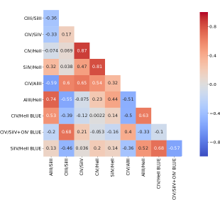
Figure 9: The correlation matrix between diagnostic ratios in BC and BLUE. The numbers in each square show the Spearman rank correlation coefficient. Red colors indicate a positive correlation, blue colors indicate a negative correlation..

4.2 Analysis of Z distributions: global inferences on sample

4.2.1 Fixed ($U$,$n_{\mathrm{H}}$)

We propagated the diagnostic intensity ratios measured on the BC and BLUE components with their lower and upper uncertainties following the relation between ratios and $Z$ in the Figures 2, for the fixed physical conditions assumed in the low- and high-ionization region. The results are reported in Table 6 and Table 7 for the BC and for the blueshifted component, respectively. The last row reports the median values of the individual sources $Z$ estimates with the sample SIQR. The distributions are shown in Figs. 10 and 11, along with a graphical presentation of each source and its associated uncertainties.

Table 6 and Table 7 permit to quantify the systematic differences that are apparent in Figs. 10 and 11. The agreement between the various estimators is in good on average (the medians scatter around $\log Z\approx 1$ by less than 0.2 dex). However, there are systematic differences between the $Z$ obtained from the various diagnostic ratios. Siiv and Aliii over Heii$\lambda$1640apparently overestimate the $Z$  by a factor 2 with respect to Civ/Heii$\lambda$1640. The out-of-scale values of Civ/Siiv and Civ/Aliii may suggest that metallicity scaling according to solar proportion may not be strictly correct (Sect. 5.6). In the case of BLUE, several estimates from Civ/Heii$\lambda$1640 strongly deviate from the ones obtained with the other ratios, due to the non-monotonic behavior of the relation between $Z$ and Civ/Heii$\lambda$1640, right in the range of metallicity that is expected. Fig. 17 shows that the non-monotonic behavior as a function of $Z$ occurs for $-1\lesssim\log U\lesssim 0$, assuming $\log$ $n_{\mathrm{H}}$= 9.

The median values of all three ratios consistently suggest high metallicity with a firm lower limit $Z\approx 5$, and in the range $10Z_{\odot}\lesssim Z\lesssim 100Z_{\odot}$, with typical values between 20 and 50 $Z_{\odot}$. There is apparently a systematic difference between BC and BLUE, in the sense that $Z$ derived from the BC is systematically higher than $Z$ from blue. The difference is small in the case of Civ/Heii$\lambda$1640 but is significant in the case of (Siiv+ Oiv])/Heii$\lambda$1640, where $Z$ from BLUE are a factor of 10 lower. We have stressed earlier that there are often absorptions affecting the BLUE of Siiv+ Oiv]/Heii$\lambda$1640. Absorptions and the blending with Cii$\lambda$1332 and Siiv BC lines make it difficult to properly define the continuum underlying the $\lambda$1400 blend at negative radial velocities. We think that the Siiv+ Oiv] BLUE intensity estimate is more of a lower limit. Another explanation might be related to the assumption of a constant density and $U$ for all sources. While there are observational constraints supporting this condition for the BC (Panda et al., 2018, 2019, 2020b), there are no strong clues to the BLUE properties, save a high ionization degree.

4.3 $Z$ for individual sources for fixed $U$, $n_{\mathrm{H}}$

Table 8 reports the $Z$ estimates for the BC, BLUE, and a combination of BC and BLUE for each individual object. The values reported are the median values of the individual objects’ estimates from the different ratios. Here the $Z$ value for each object is computed by vetting the ratios according to concordance. If the discordance is not due on physical ground, but rather to instrumental problems (for example, contamination by absorption lines, non linear dependence on $Z$ of some ratios), a proper strategy is to use estimators such as the median that eliminate discordant values even for small sample sizes ($n\geq 3$). Measuring medians and SIQR is an efficient way to deal with the measurements of large samples of objects. All estimates $\log Z\lesssim 0$ were excluded, as either the product of heavy absorptions (Siiv+Oiv]/Heii$\lambda$1640) or of difficulties in relating the ratio (Civ/Heii$\lambda$1640) to $Z$; apart from J211651.48+044123.7, the upper uncertainty of the negative estimates is so large that $Z$ is actually unconstrained. The difference between BLUE and BC is even more evident: the median (last row) indicates a factor $\approx 6$ difference between BLUE and BC. The BC suggests a median $Z\approx 60Z_{\odot}$, while the BLUE $Z\approx 10Z_{\odot}$. The assumption that the wind and disk component have the same $Z$ in each object is a reasonable one, with the caveats mentioned in Sect. 5.6. Therefore the two estimates, for BLUE and BC could be considered two independent estimators of $Z$. If the two estimates are combined for each individual object, $10Z_{\odot}\lesssim Z\lesssim 100Z_{\odot}$, with a median value of $Z\approx 20Z_{\odot}$.

There is a good agreement between the $Z$ median estimates from the BC and BLUE of Civ, $\log Z\approx 1.27$ vs $\log Z\approx 1.13$, respectively (Tables 6 and 7). Ignoring Siiv+Oiv] and Aliii, the $Z\approx 20Z_{\odot}$ value derived for the Civ BC is not affected by a possible enhancement of [Si/C] and [Al/C] with respect to the solar values. If the Carbon abundance is used as a reference, the BC $Z$ estimate from Aliii and Siiv could point toward a selective enhancement of Si and Al with respect to C.

The disagreement between BLUE and BC $Z$ estimates rests on the blueshifted component of Siiv+ Oiv]. The disagreement between the $Z$ estimates from ratios involving Siiv+Oiv] BC and BLUE might be explained if one considers that the measurement of the Siiv+Oiv] BLUE is most problematic and the Siiv+Oiv]  intensity might be systematically underestimated.

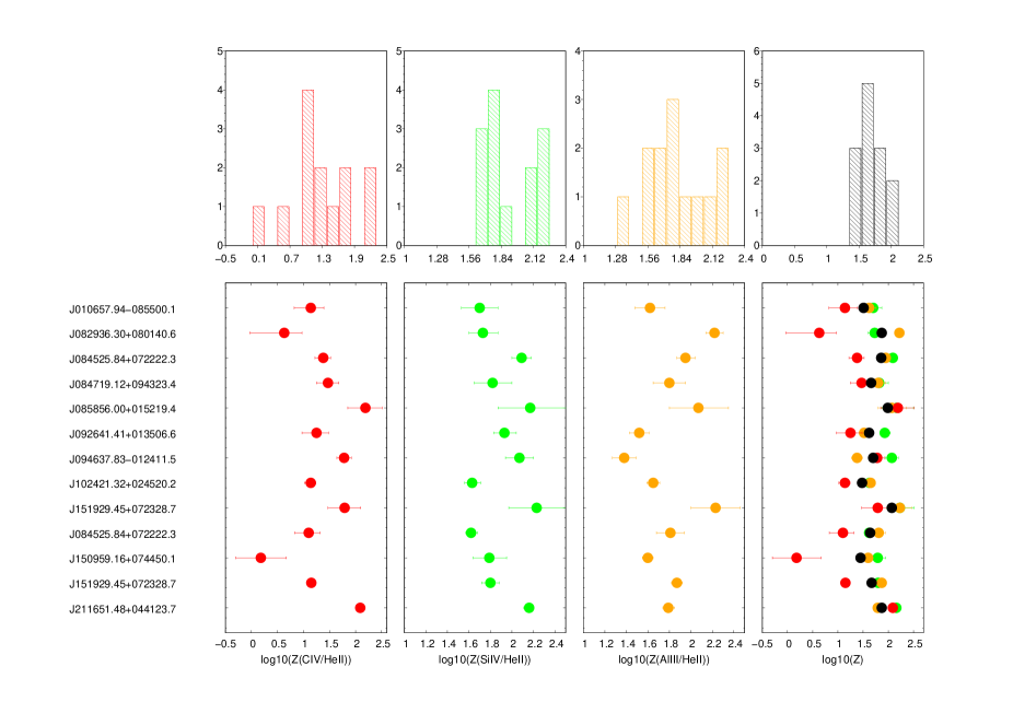
Figure 10: (Upper panel) Distribution of metallicity measurements for broad component obtained from ratios Civ/Heii$\lambda$1640 (red), Siiv/Heii$\lambda$1640 (green), Aliii/Heii$\lambda$1640 (orange) and the mean metallicity obtained from all ratios (black). (Lower panel) Results and associated uncertainties for individual sources with the same color-coding as histograms. The last panel contains all metallicity measurements and the mean of them for each object.

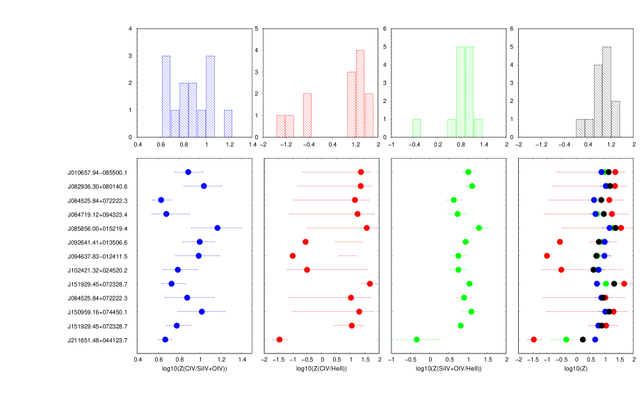
Figure 11: (Upper panel) Distribution of metallicity measurements for blue component obtained from ratios: Civ/Siiv+Oiv] (blue), Civ/Heii$\lambda$1640 (red), Siiv+Oiv]/Heii$\lambda$1640 (green) and the mean metallicity obtained from all ratios (black). (Lower panel) Results and associated uncertainties for individual sources with the same color-coding as histograms. The last panel contains all metallicity measurements and the mean of them for each object.

Table 6: Metallicity ($\log Z$) of the BC assuming fixed $U$, $n_{\mathrm{H}}$ 

SDSS JCODE	Civ/Heii$\lambda$1640	Siiv/Heii$\lambda$1640	Aliii/Heii$\lambda$1640
J010657.94-085500.1	1.16 ${}_{-0.33}^{+0.26}$	1.85 ${}_{-0.20}^{+0.20}$	1.7 ${}_{-0.15}^{+0.16}$
J085856.00+015219.4	2.22 ${}_{-0.35}^{+0.36}$	2.41 ${}_{-0.36}^{+0.59}$	2.2 ${}_{-0.29}^{+0.31}$
J082936.30+080140.6	0.63 ${}_{-0.65}^{+0.36}$	1.89 ${}_{-0.15}^{+0.16}$	2.36 ${}_{-0.09}^{+0.10}$
J084525.84+072222.3	1.41 ${}_{-0.16}^{+0.14}$	2.31 ${}_{-0.11}^{+0.11}$	2.07 ${}_{-0.09}^{+0.10}$
J084719.12+094323.4	1.50 ${}_{-0.23}^{+0.20}$	1.99 ${}_{-0.19}^{+0.21}$	1.91 ${}_{-0.17}^{+0.17}$
J092641.41+013506.6	1.27 ${}_{-0.29}^{+0.24}$	2.12 ${}_{-0.12}^{+0.12}$	1.59 ${}_{-0.10}^{+0.11}$
J094637.83-012411.5	1.80 ${}_{-0.14}^{+0.15}$	2.29 ${}_{-0.15}^{+0.16}$	1.44 ${}_{-0.13}^{+0.12}$
J102421.32+024520.2	1.16 ${}_{-0.12}^{+0.11}$	1.77 ${}_{-0.08}^{+0.09}$	1.74 ${}_{-0.06}^{+0.07}$
J102606.67+011459.0	1.82 ${}_{-0.32}^{+0.30}$	2.49 ${}_{-0.32}^{+0.51}$	2.38 ${}_{-0.26}^{+0.27}$
J114557.84+080029.0	1.12 ${}_{-0.27}^{+0.22}$	1.96 ${}_{-0.18}^{+0.19}$	1.92 ${}_{-0.15}^{+0.15}$
J150959.16+074450.1	0.19 ${}_{-0.47}^{+0.49}$	1.76 ${}_{-0.07}^{+0.06}$	1.69 ${}_{-0.06}^{+0.05}$
J151929.45+072328.7	1.18 ${}_{-0.09}^{+0.08}$	1.97 ${}_{-0.09}^{+0.08}$	1.98 ${}_{-0.05}^{+0.05}$
J211651.48+044123.7	2.11 ${}_{-0.04}^{+0.04}$	2.39 ${}_{-0.06}^{+0.06}$	1.9 ${}_{-0.06}^{+0.06}$
Median	1.27 $\pm$ 0.32	1.99$\pm$ 0.21	1.91$\pm$ 0.18

Note. — Columns: (1) SDSS identification, (2), (3) and (4) metallicity values for Civ/Heii$\lambda$1640  Siiv+Oiv]/Heii$\lambda$1640 and Aliii/Heii$\lambda$1640 with uncertainties.

Table 7: Metallicity ($\log Z$) of BLUE assuming fixed $U$, $n_{\mathrm{H}}$ 

SDSS JCODE	Siiv+Oiv]/Heii$\lambda$1640	Civ/Siiv+Oiv]	Civ/Heii$\lambda$1640
J010657.94-085500.1	1.00 ${}_{-0.16}^{+0.12}$	0.88 ${}_{-0.12}^{+0.14}$	1.34 ${}_{-1.99}^{+0.34}$
J085856.00+015219.4	1.26 ${}_{-0.13}^{+0.20}$	1.12 ${}_{-0.21}^{+0.23}$	1.55 ${}_{-2.05}^{+0.35}$
J082936.30+080140.6	1.10 ${}_{-0.16}^{+0.14}$	1.03 ${}_{-0.19}^{+0.16}$	1.33 ${}_{-2.14}^{+0.41}$
J084525.84+072222.3	0.62 ${}_{-0.19}^{+0.20}$	0.63 ${}_{-0.09}^{+0.09}$	1.13 ${}_{-2.07}^{+0.50}$
J084719.12+094323.4	0.72 ${}_{-0.24}^{+0.27}$	0.68 ${}_{-0.15}^{+0.21}$	1.22 ${}_{-2.32}^{+0.59}$
J092641.41+013506.6	0.93 ${}_{-0.14}^{+0.11}$	0.99 ${}_{-0.16}^{+0.14}$	-0.56 ${}_{-0.46}^{+1.93}$
J094637.83-012411.5	0.74 ${}_{-0.18}^{+0.20}$	0.98 ${}_{-0.22}^{+0.20}$	-0.99 ${}_{-1.06}^{+2.16}$
J102421.32+024520.2	0.73 ${}_{-0.20}^{+0.24}$	0.78 ${}_{-0.14}^{+0.19}$	-0.52 ${}_{-0.65}^{+2.10}$
J102606.67+011459.0	1.02 ${}_{-0.12}^{+0.11}$	0.73 ${}_{-0.10}^{+0.12}$	1.67 ${}_{-0.31}^{+0.24}$
J114557.84+080029.0	0.89 ${}_{-0.22}^{+0.19}$	0.87 ${}_{-0.20}^{+0.25}$	0.99 ${}_{-2.12}^{+0.70}$
J150959.16+074450.1	1.07 ${}_{-0.21}^{+0.18}$	1.01 ${}_{-0.23}^{+0.22}$	1.28 ${}_{-2.28}^{+0.52}$
J151929.45+072328.7	0.79 ${}_{-0.06}^{+0.07}$	0.78 ${}_{-0.11}^{+0.13}$	1.02 ${}_{-0.59}^{+0.40}$
J211651.48+044123.7	-0.57 ${}_{-0.43}^{+0.81}$	0.66 ${}_{-0.05}^{+0.06}$	-1.46 ${}_{-0.23}^{+0.27}$
Medians	0.89 $\pm$ 0.15	0.87$\pm$ 0.13	1.13$\pm$ 0.92

Note. — Columns: (1) SDSS identification, (2), (3) and (4) metallicity values for Siiv+Oiv]/Heii$\lambda$1640  Civ/Siiv+Oiv] and Civ/Heii$\lambda$1640 with uncertainties.

Table 8: Metallicity ($\log Z$) of individual quasars assuming fixed $U$, $n_{\mathrm{H}}$ 

SDSS JCODE	BC	BLUE	Combined
J010657.94-085500.1	1.70 $\pm$ 0.34	1.00 $\pm$ 0.23	1.34 $\pm$ 0.35
J082936.30+080140.6	1.89 $\pm$ 0.86	1.10 $\pm$ 0.15	1.33 $\pm$ 0.43
J084525.84+072222.3	2.07 $\pm$ 0.45	0.63 $\pm$ 0.25	1.41 $\pm$ 0.72
J084719.12+094323.4	1.91 $\pm$ 0.25	0.72 $\pm$ 0.27	1.50 $\pm$ 0.60
J085856.00+015219.4	2.22 $\pm$ 0.11	1.26 $\pm$ 0.21	2.20 $\pm$ 0.48
J092641.41+013506.6	1.59 $\pm$ 0.42	0.93 $\pm$ 0.77	1.27 $\pm$ 0.33
J094637.83-012411.5	1.80 $\pm$ 0.42	0.74 $\pm$ 0.99	1.44 $\pm$ 0.53
J102421.32+024520.2	1.74 $\pm$ 0.30	0.73 $\pm$ 0.65	1.16 $\pm$ 0.51
J102606.67+011459.0	2.38 $\pm$ 0.33	1.02 $\pm$ 0.47	1.82 $\pm$ 0.68
J114557.84+080029.0	1.92 $\pm$ 0.42	0.89 $\pm$ 0.06	1.12 $\pm$ 0.52
J150959.16+074450.1	1.69 $\pm$ 0.78	1.07 $\pm$ 0.14	1.28 $\pm$ 0.34
J151929.45+072328.7	1.97 $\pm$ 0.40	0.79 $\pm$ 0.12	1.18 $\pm$ 0.59
J211651.48+044123.7	2.11 $\pm$ 0.24	0.66 $\pm$ …	2.11 $\pm$ 0.34
Median	1.91 $\pm$ 0.16	0.89 $\pm$ 0.12	1.34 $\pm$ 0.11

Note. — Columns: (1) SDSS identification, (2), (3) and (4) metallicity medians for BC, BLUE and the combination of the two, with uncertainties. Column (5) yields the number of ratios used for the BLUE estimates. No uncertainty is reported for BLUE of SDSS J211651.48+044123.7 (catalog ) since only one ratio was used.

4.4 Estimates of $Z$ relaxing the constraints on $U$ and $n_{\mathrm{H}}$

We computed the $\chi^{2}$ in the following form, to identify the value of the metallicity for median values of the diagnostic ratios and for the diagnostic ratios of individual objects relaxing the assumption of fixed density and ionization parameters. For each object $k$, and for each component $c$, we can write:

$$\chi^{2}_{\mathrm{kc}}(n_{\mathrm{H}},U,Z) = \sum_{\mathrm{{i}}}w_{\mathrm{ci}}\left(\frac{R_{\mathrm{kci}}-R_{\mathrm{kci,mod}}(n_{\mathrm{H}},U,Z)}{\delta R_{\mathrm{kci}}}\right)^{2}$$ (8)

where the summation is done over the available diagnostic ratios, and the $\chi^{2}$ is computed with respect to the results of the CLOUDY simulations as a function of $U$, $n_{\mathrm{H}}$, and $Z$ (subscript ‘mod’). Weights $w_{\mathrm{ci}}=1$ were assigned to Civ/Heii$\lambda$1640, Siiv/Heii$\lambda$1640, and Aliii/Heii$\lambda$1640; $w_{\mathrm{ci}}=0$ or 0.5 were assigned to Civ/Aliii and and Civ/Siiv. For BLUE, the three diagnostic ratios were all assigned $w_{\mathrm{ci}}=1$. The $Z$ estimates for the BC are based on the three ratios involving Heii$\lambda$1640 normalization.

To gain a global, bird’s eye view of the $Z$ dependence on the physical parameters, Fig. 12 shows the 3D space $U$, $n_{\mathrm{H}}$, $Z$. Each point in this space corresponds to an element of the grid of CLOUDY the parameter space and is consistent with the minimum $\chi^{2}$ within the uncertainties at 1$\sigma$ confidence level. The case shown in the panels of Fig. 12 is the one with the median values of the sample objects.

The distribution of the data points is constrained in a relatively narrow range of $U$, $n_{\mathrm{H}}$, $Z$, at very high density, low ionization, and high metallicity. Within the limit in $U$, $n_{\mathrm{H}}$, the distribution of $Z$ is flat and thin, around $Z\sim 50-100Z_{\odot}$. This implies that, for a change of the $U$ and $n_{\mathrm{H}}$ within the limits allowed by the data, the estimate of $Z$ is stable and independent on $U$ and $n_{\mathrm{H}}$. Table 8 reports the individual $Z$ estimates and the SIQR for the sources in the sample (the last row is the median).

The allowed parameter space volume for BLUE is by far less constrained. The right panel of Fig. 12 shows the parameter space for the $Z$ estimates from the 3 BLUE intensity ratios. The condition on the $\chi^{2}$ distribution is the same, as used for the BC, namely that the data points all satisfy the condition $\chi^{2}\leq\chi^{2}_{\mathrm{min}}+1$. A similar shape is obtained if we consider the condition that all the 3 ratios agree with the ones predicted by the model within 1$\sigma$. The spread in ionization and density is very large, although the concentration of data points is higher in the case of low $n_{\mathrm{H}}$ ($\log$ $n_{\mathrm{H}}$$\sim$ 8-9 [cm^-3]) and high ionization ($\log U\sim 0$). At any rate the spread of the data points indicate that solutions at low ionization and high density are also possible. The results for individual sources tend to disfavor this scenario for the wide majority of the objects, but the properties of the gas emitting the BLUE component are less constrained than the ones of the gas emitting the BC. What is missing for BLUE is especially a firm diagnostic of density that in the case of BC is provided mainly by the ratio Aliii/Heii$\lambda$1640. Results on $Z$ are however as stable as for the BC, even if the dispersion is larger, and suggest values in the range $10\lesssim Z\lesssim 50Z_{\odot}$.

Summing up, all meaningful estimators converge toward high $Z$ values, definitely super-solar, with $Z\gtrsim 10Z_{\odot}$. Ratios Civ/Siiv significantly less than $<1$ are predicted in the parameter space. Siiv/Heii$\lambda$1640 seems to give the largest estimates of $Z$. Also the high Aliii/Civ requires high values of $Z$. A conclusion has to be tentative, considering the possible systematic errors affecting the estimates of the Civ and Siiv intensities: for Civ, the BC in the most extreme cases is often buried under an overwhelming BLUE; a fit is not providing a reliable estimate of the BC (by far the fainter component) but provides a reliable BLUE intensity; for Siiv we may overestimate the intensity due to “cancellation” of the BLUE by absorptions. This said, the present data are consistent with the possibility of a selective enhancement of Al and Si, as already considered by Negrete et al. (2012). The issue will be briefly discussed in Sect. 5.

At any rate, the absence of correlation between BLUE and BC parameters (Fig. 9), the difference in the diagnostic ratios and differences in inferred $Z$, as well as the results for individual sources described below justify the approach followed in the paper to maintain a separation between BLUE and BC. The meaning of possible systematic differences between the BC and BLUE are further discussed in §5.

4.4.1 Individual sources

BC

The best $n_{\mathrm{H}}$, $U$, and $Z$ for each object have been obtained by minimizing the $\chi^{2}$ as defined in Eq. 8, and they are reported in Table 9. The $\chi^{2}_{\mathrm{min}}$ values are listed in the second Column of Tab. 9. At the side of each value there is the uncertainty range for each parameter defined from volume in the parameter space satisfying the condition $\chi^{2}\approx\chi^{2}_{\mathrm{min}}+1$. In other words, the choice of the best physical conditions was obtained by minimizing the sum of the deviations between the model predictions and the observer diagnostic ratios. The last two rows list the minimum $\chi^{2}$ values for the median (with the SIQR of the sample from Table 5) and for the median of the values reported for individual sources in Table 9. The obtained values of $Z$ cover the range $5\lesssim Z\lesssim 100$, with 9 out of 13 sources with $50\lesssim Z\lesssim 100Z_{\odot}$, and medians of intensity ratios yielding $Z\sim 50Z_{\odot}$. There is some spread in the ionization parameter values, $-4\lesssim U\lesssim-1$, but in most cases $U$ indicates low or very low ionization level. The Hydrogen density is very high: in only a few cases $\log$$n_{\mathrm{H}}$$\sim 10-11$, and in several cases $n_{\mathrm{H}}$ reaches 10¹⁴ cm^-3. The median values from the ratios are $\log U=-2.25$, $\log$ $n_{\mathrm{H}}$=13.75 (with a range 12.5 – 14), therefore validating the original assumption of $\log U=-2.5$, $\log$ $n_{\mathrm{H}}$= 12 for fixed physical condition. The results for individual sources confirm the scenario of Fig. 12 for the wide majority of the sample sources. The higher $n_{\mathrm{H}}$ values are consistent with recent inferences for the low-ionization BLR derived from Temple et al. (2020), based on the FeIII UV emission which is especially prominent in the UV spectra of xA quasars (Martínez-Aldama et al., 2018). It is interesting to note that two of the borderline objects (Aliii/Siiii]$\approx 0.5$, Ciii]/Siiii]$\approx 1$) show higher values of the ionization parameter ($\log U\approx-1.--1.5$).

Large ($\gg 1$) values of $\chi^{2}_{\mathrm{min}}$ are associated with cases in which the BC components of Aliii and/or of Siiv are strong with respect to the BC of Civ, and are further increased by small uncertainty ranges (which are more likely to occur if a line is strong). Intensity ratios Civ/Aliii$\lesssim 1$ and Civ/Siiv$\lesssim 1$ are reproduced by photoionization simulations in conditions of very low ionization. The ratio Civ/Aliii tend to decrease with increasing $Z$, although the trend is steep in the case of $\log$ $n_{\mathrm{H}}$$\sim$ 9, and more shallow at the higher densities appropriate for the BC emission (Appendix B). However, high values of the Aliii and Siiv+Oiv] over Heii ratios induced by overabundances could bias the $U$ and lower its values.

BLUE

The inferences are less clear from BLUE (Table 10, organized like Table 9). In most cases, the permitted volume in the 3D parameter space for individual sources covers a broad range in $U$ and $n_{\mathrm{H}}$ as for the median (Fig. 12). Fig. 12 shows that there is a strip of $\chi^{2}$ values statistically consistent with the minimum $\chi^{2}$ that crosses the full domain of the parameter space. Along this strip of permitted values $n_{\mathrm{H}}$ and $U$ are linearly dependent, with $\log U\approx-0.5\cdot n_{\mathrm{H}}+4$ for the median composite ratios. In most sources the $U$ value implies a high degree of ionization, $-1\lesssim\log U\lesssim 0$, but in three cases (for example SDSS J150959.16+074450.1 (catalog )) there is apparently a low-ionization solution with $U$ comparable to that of the low-ionization BLR. The median are $\log$$n_{\mathrm{H}}$$\sim 7.75$, $\log$U $\sim$-0.5, close to the values that we assumed for the fixed ($U$, $n_{\mathrm{H}}$) approach. The results on metallicity suggest in most cases $Z\gtrsim 20Z_{\odot}$. However, within 1 SIQR from the minimum $\chi^{2}$, $Z$ values up to 30 are also possible.

$Z$ values from BLUE are systematically lower than the those from BC. The medians differ by a factor of 2. However, a Welch t-test (Welch, 1947) fails to detect a significant difference between the average values of the metallicity for the two components: $t\approx 0.86$ for 5 degrees of freedom (computed using the Welch-Satterthwaite equation) implies a significance of just 80%. Three cases in which the disagreement is large, more than a factor 5, namely J084525.84+072222.3, J084719.12+094323.4, J102606.67+011459.0 are apparently not strongly affected by absorption lines, but the constraints from Table 10 and Table 9 are poor, implying that also for BLUE the $Z$ could be much higher. Therefore, we cannot substantiate any claim of a systematic difference between BLUE and BC $Z$ estimates.

The $Z$,  $U$, $n_{\mathrm{H}}$ parameter space occupation of xA quasars

In summary, the low-ionization BLR of xA sources seems to be consistently characterized by low ionization, extremely high density and very high metallicity, under the assumption that $Z$ scales with the solar chemical composition. Diagnostics on BLUE is less constraining, and measurements are more difficult. The 0-order results are however consistent again with high metallicity $Z\gtrsim 5Z_{\odot}$.

The 3D distribution in Fig. 12 indicates that, although there might be a large range of uncertainty in the $U$ and $n_{\mathrm{H}}$ especially for BLUE, the $Z$ values tend to remain constrained within a narrow strip around a well-defined $Z$, parallel to the $U$, $n_{\mathrm{H}}$ plane. In other words, $Z$ estimates should be stable, as they are not strongly dependent on the assumed physical parameters.

Comparing the individual $Z$ estimates for fixed and free $n_{\mathrm{H}}$ and $U$ (Cols. 2 of Table 6 and Table 9) for the BC, the agreement is good, with a median difference of 0.22 and a SIQR of 0.15, with the fixed $n_{\mathrm{H}}$ and $U$ being therefore a factor $\approx 1.65$ higher than the one derived assuming a free $n_{\mathrm{H}}$ and $U$. Two sources (J151929.45+072328.7 (catalog ) and J114557.84+080029.0 (catalog )) show a large disagreement, in the sense that the $Z$ values leaving $U$ and $n_{\mathrm{H}}$ free are much lower. These $Z$ estimates are however highly uncertain, with a shallow $\chi^{2}$ distribution around the minimum especially for J151929.45+072328.7 (catalog ). For this object the maximum metallicity covered by the simulations $Z=1000Z_{\odot}$ is still consistent within the uncertainties.

Table 9: $Z$, $U$, $n_{\mathrm{H}}$ of individual sources and median derived from the BC

SDSS JCODE	$\chi^{2}_{\mathrm{min}}$	$\log Z$ [$Z_{\odot}$]	$\delta\log Z$ [$Z_{\odot}$]	$\log U$	$\delta\log U$	$\log$ $n_{\mathrm{H}}$	$\delta\log$ $n_{\mathrm{H}}$
(1)	(2)	(3)	(4)	(5)	(6)	(7)
J010657.94-085500.1	2.6894	1.7	0.7 – 1.7	-2.00	-2.75 – -1.25	13.50	12.00 – 14.00
J082936.30+080140.6	6.6414	1.3	0.7 – 2.7	-4.00	-4.00 – -3.50	14.00	12.75 – 14.00
J084525.84+072222.3	13.700	1.7	1.0 – 3.0	-1.75	-3.75 – -0.25	14.00	12.00 – 14.00
J084719.12+094323.4	1.7004	1.7	1.0 – 2.0	-2.25	-2.50 – -1.50	13.75	12.50 – 14.00
J085856.00+015219.4	0.0012	2.0	1.7 – 2.7	-2.25	-3.00 – -1.75	12.50	12.00 – 14.00
J092641.41+013506.6	1.7982	1.7	1.7 – 2.0	-1.50	-1.75 – -1.00	14.00	13.50 – 14.00
J094637.83-012411.5	0.3253	1.7	1.7 – 2.3	-1.00	-1.25 – -0.75	12.25	11.75 – 14.00
J102421.32+024520.2	15.819	1.7	1.3 – 2.0	-2.25	-3.00 – -1.50	13.50	12.75 – 14.00
J102606.67+011459.0	1.5020	2.0	1.7 – 2.3	-1.75	-2.50 – -0.75	14.00	12.50 – 14.00
J114557.84+080029.0	6.6174	0.7	0.7 – 2.0	-3.75	-3.75 – -1.25	14.00	12.25 – 14.00
J150959.16+074450.1	45.287	1.3	0.5 – 2.0	-1.75	-0.50 – -3.50	13.75	12.25 – 14.00
J151929.45+072328.7	29.220	0.7	0.3 – 3.0	-3.75	-4.00 – -2.75	14.00	11.00 – 14.00
J211651.48+044123.7	1.4476	2.0	1.7 – 2.0	-2.00	-2.00 – -0.75	12.25	10.75 – 12.25
$\mu_{\frac{1}{2}}$(Ratios)	1.9914	1.7	0.7 – 2.0	-2.25	-2.75 – -1.25	13.75	12.50 – 14.00
$\mu_{\frac{1}{2}}$(Objects)	…	1.7	1.5 – 1.9	-2.00	-2.25 – -1.75	13.75	13.50 – 14.00

Table 10: $Z$, $U$, $n_{\mathrm{H}}$ of individual sources and median derived from BLUE

SDSS JCODE	$\chi^{2}_{\mathrm{min}}$	$\log Z$ [$Z_{\odot}$]	$\delta\log Z$ [$Z_{\odot}$]	$\log U$	$\delta\log U$	$\log$ $n_{\mathrm{H}}$	$\delta\log$ $n_{\mathrm{H}}$
(1)	(2)	(3)	(4)	(5)	(6)	(7)
J010657.94$-$085500.1	0.00985	1.70	0.70 – 1.7	0.75	-1.5 – 0.75	7.75	7.50 – 9.75
J082936.30+080140.6	0.01506	1.30	1.00 – 1.70	-0.25	-2.0 – -0.00	8.00	7.75 – 12.25
J084525.84+072222.3	0.00143	1.0	0.00 – 2.30	-1.50	-2.50 – -1.25	7.25	7.00 – 11.25
J084719.12+094323.4	0.00097	1.00	0.00 – 3.00	-2.24	-2.50 – 0.75	8.75	7.50 – 11.50
J085856.00+015219.4	0.00305	1.70	1.0 – 2.00	0.50	-1.75 – 0.50	8.25	7.00 – 11.75
J102606.67+011459.0	0.00111	0.70	0.70 – 3.00	-1.00	-2.50 – -0.5	9.25	8.25 – 11.25
J114557.84+080029.0	0.00164	1.30	0.30 – 1.70	-2.50	-2.50 – 0.25	11.50	7.25 – 12.50
J150959.16+074450.1	0.00288	1.30	0.30 – 2.00	-2.00	-2.75 – 0.75	11.75	7.00 – 13.75
J151929.45+072328.7	0.00032	0.30	0.30 – 1.30	-0.50	-0.75 – -0.25	10.00	7.75 – 10.25
$\mu_{\frac{1}{2}}$(Ratios)	0.07336	1.30	1.0 – 1.30	-0.50	-0.50 – -0.50	7.75	7.75 – 8.00
$\mu_{\frac{1}{2}}$(Objects)	…	1.30	1.15 – 1.45	-1.00	-0.125 – -1.875	8.75	7.75 – 9.75

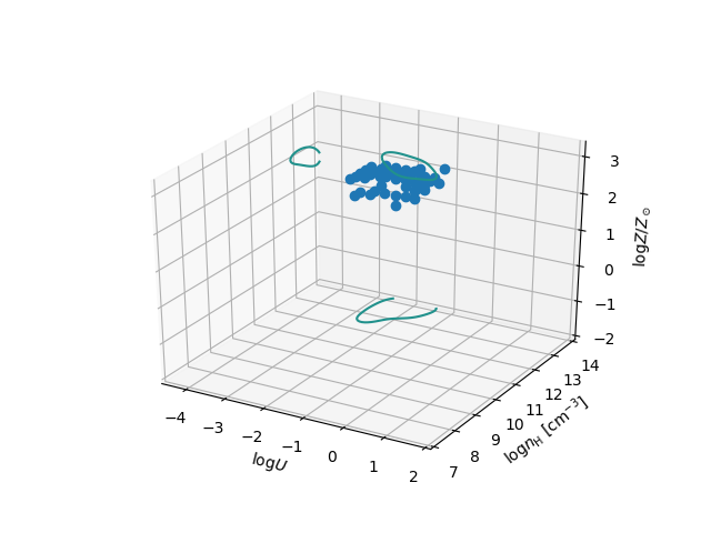
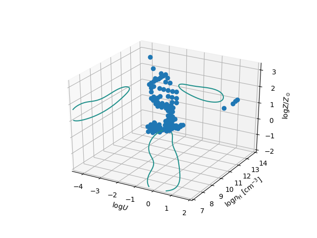
Figure 12: The parameter space $n_{\mathrm{H}}$, $U$, $Z$. Left: data points in 3D space are elements in the grid of the parameter space selected for not being different from $\chi^{2}_{\mathrm{min}}$ by more than $\delta\chi^{2}\approx 1$, computed from the emission line ratios measured for the BC and referring to the median values in Table 5. Right: same for the BLUE component, also including the condition that that the data points are in agreement with the three diagnostic ratios within the SIQR of the median estimate from Table 5. The individual contour line was smoothed with a Gaussian kernel.

5 Discussion

5.1 A method to estimate $Z$

The determination of the metal content of the broad line emitting region of xA quasars was made possible by the following procedure:

1. the estimation of an accurate redshift. Even if all lines are affected by significant blueshifts which reduce the values of measured redshift, in the absence of information from the H$\beta$ spectral range the Aliii and the $\lambda$1900 blend can be used as proxies of proper redshift estimators. The blueshifts are the smallest in the intermediate ionization lines at $\lambda$1900 (del Olmo et al., in preparation).

2. the separation of the BC and BLUE, for Civ and the $\lambda$1400 blend. The line width of the individual components of the Aliii doublet can be used as a template BC. The component BLUE is defined as the excess emission on the blue side of the BC.

3. a first estimate of metallicity can be obtained from the assumption that the low-ionization BLR associated with the BC and wind/outflow component associated with BLUE can be described by similar physical conditions in different objects. Several diagnostic ratios can be associated with the intensity ratios predicted by an array of photoionization simulations, namely

   • for the BC: Aliii/Heii$\lambda$1640, Civ/Heii$\lambda$1640, Siiv/Heii$\lambda$1640, assuming ($\log U$, $\log$$n_{\mathrm{H}}$) = (-2.5,12) or ($\log U$, $\log$$n_{\mathrm{H}}$) = (-2.5,13)

   • for the BLUE: Civ/Heii$\lambda$1640, Siiv+Oiv]/Heii$\lambda$1640, Civ/Siiv+Oiv]  assuming ($\log U$, $\log$$n_{\mathrm{H}}$) = (0,9).

4. Estimates can be refined for individual sources relaxing the constant ($\log U$, $\log$$n_{\mathrm{H}}$) assumptions. Tight constraints can be obtained for the BC. The BLUE is more problematic, because of both observational difficulties and the absence of unambiguous diagnostics.

Our method relies on ratios involving Heii$\lambda$1640 that have not been much considered in previous literature. In addition, we have considered fixed SED, turbulence (equal to 0), and column density in the simulations ($N_{\rm c}$= 10²³) as fixed. The role of turbulence is further discussed in Sect. 5.5, and is found to be not relevant unlike in the case of Feii emission in the optical spectral range, where effects of self- and Ly$\alpha$-fluorescence are important, (e.g., Verner et al., 1999; Panda et al., 2018), while the $N_{\rm c}$ effect is most likely negligible.

Extension of the method to the full Population A is a likely possibility, since we do not expect a very strong effect of the SED on the metallicity estimate, as long as the SED has a prominent big blue bump, as it seems to be case for Population A. The role of SED is likely important if the method has to be extended to sources of Pop. B along the main sequence. At least two SED cases should be considered, if the aim is to apply the method presented in this paper to a large sample of quasars.

Intensity ratios involving Heii$\lambda$1640 are difficult to measure in the xA spectra, but may be more accessible for Population B spectra. Ferland et al. (2020) have shown significant differences in the SED as a function of $L/L_{\rm Edd}$, with a much flatter SED at low $L/L_{\rm Edd}$. The extension to Pop. B would therefore require a new dedicated array of simulations.

Metallicity increases with $M_{\rm BH}$ (Matsuoka et al., 2011), and ratios involving Nv are apparently correlated with $L/L_{\rm Edd}$, suggesting a delay of $\sim 10^{8}$ for the onset of nuclear activity after star forming events …Difficulties in moddeling of Siiv+Oiv] are generally known in the literature (cite ???). Siiv is probably overestimated, while Oiv] is underestimated (why???). Moreover, the Siiv+Oiv] blend is strongly affected by absorption (show in which figures we can see it???). The BC emission in Siiv+Oiv] blend is dominated by Siiv due to collisional deexcitation of the intercombination Oiv] (cite ???). The BLUE component emission comes from an inextricable contribution of both Siiv+Oiv]. Table 5. Measured Quantities on Composite Spectra - Pop. A Average fluc values lya and nv - Sulentic et al.: Spectra of Quasars at $\approx$ 2.3. We must preliminarily point out that great care should be exerted in analyzing data based on the Nv 1240/Civ 1549 and Nv 1240/Heii$\lambda$1640 ratios because: (1) the intensity of the Nv 1240 line is very difficult to estimate unambiguously unless a reliable model of the Ly$\alpha$ wings are build as done… L. E. Simon and F. Hamann: Metallicity and FIR luminosity of high-z QSOs - Figure 3.Gaussian fits for Ly$\alpha$,andNVin the left panels and CIVin theright panels for each normalized composite spectrum. As shown in Figure 8, low-z AGNs with log[L/L Edd ] $<-1.5$ (that is not covered in the high-z sample) show systematically lower N V /C IV flux ratios, leading to the more evident dependence on L/L Edd . FROM SHIN 12: R ESULTS OF S PEARMAN ’ S RANK - ORDER CORRELATION TEST - N V /C IV AND N V /He II. FROM SHIN 12: In Figure 5 (bottom panel) we compare the N V 1240 flux and the sum of the Si IV 1397 and O IV ] 1402 fluxes, which are used as a numerator of metallicity indicators. Again a clear positive correlation is present between them, with a somewhat larger scatter than that shown in the comparison between the C IV and He II fluxes. This larger scatter is partly caused by the fact that the N V flux depends on Z BLR as well as the relative abundance of N V (see, e.g., Matsuoka et al. 2011b; Araki et al. 2012), while the sum of the Si IV and O IV ] fluxes mainly depends on Z BL

5.2 Accretion parameters of sample sources

The bolometric luminosity has been computed assuming a flat $\Lambda$CDM cosmological model with $\Omega_{\Lambda}$ = 0.7, $\Omega_{m}$ = 0.3, and H₀ = 70 km s^-1 Mpc^-1. Following Marziani & Sulentic (2014) we decided to use Aliii as virial broadening estimator for computing the $M_{\rm BH}$. Our estimates adopt two different scaling laws: (1) the scaling laws of Vestergaard & Peterson (2006) for Civ and a second, unpublished one based on Aliii (del Olmo et al., in preparation). Eddington ratios have been obtained using the Eddington luminosity $L_{\mathrm{Edd}}\approx 1.3\times 10^{38}(M_{\mathrm{BH}}/M_{\odot})$ erg s^-1. The luminosity range of the sample is very limited, less than a factor 3, $46.8\lesssim\log L\lesssim 47.3$, in line with the requirement of similar redshift and high flux values. Correspondingly, the $M_{\rm BH}$ and the Eddington ratio are constrained in the range $8.8\lesssim\log$$M_{\rm BH}$$\lesssim 9.5$ and $-0.55\lesssim\log$ $L/L_{\rm Edd}$$\lesssim 0.18$, respectively. The $M_{\rm BH}$ sample dispersion is small, with $\log$ $M_{\rm BH}$$\sim$ 9.4 $\pm 0.2$ [$M_{\odot}$]. The scatter in $M_{\rm BH}$ and $L/L_{\rm Edd}$ is reduced to $\approx$ 0.1 dex if we exclude one object with the lowest $M_{\rm BH}$ and highest $L/L_{\rm Edd}$. Applying a small correction (10%) to the FWHM to account for an excess broadening in Aliii due to non-virial motions will decrease the $M_{\rm BH}$ by 0.1 dex (as found by Negrete et al. 2018 for H$\beta$), and increase $L/L_{\rm Edd}$ correspondingly. If this correction is applied the median $L/L_{\rm Edd}$ is $\approx$0.6. Using the Civ BC FWHM as a virial broadening estimator further decreases the $M_{\rm BH}$ median estimate by 0.1 dex. The accretion parameters are consistent with extreme quasars of Population A at high mass and luminosity; they are mainly at the low $L/L_{\rm Edd}$  end of Sample 3 (based on $M_{\rm BH}$ estimates from Aliii) of Marziani & Sulentic (2014). The small dispersion in physical properties of the present sample ($0.2$ dex) focuses the analysis on properties that may differ for fixed accretion parameters, and fixed ratio of radiation and gravitation forces, perhaps related to different enrichment histories.

5.2.1 Correlation between diagnostic ratios and AGN physical properties

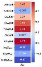
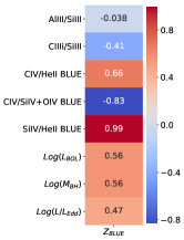
Figure 13: Left panel: the correlation matrix between $Z$ computed for the BC, and BC diagnostic ratios assuming fixed $n_{\mathrm{H}}$ and $U$ along with log of bolometric luminosity, log of black hole mass and log of Eddington ratio. Right panel: Same, but for the BLUE component. The numbers in each square show the Spearman rank correlation coefficient. The color hue is proportional to the correlation, from dark blue (strong negative correlation) to red (strong positive correlation).

Considering the small dispersion in $M_{\rm BH}$, $L/L_{\rm Edd}$ and bolometric luminosity, it is hardly surprising that none of the ratios utilized in this paper is significantly correlated with the accretion parameter. The highest degree of correlation is seen between $L/L_{\rm Edd}$ and Civ/Aliii, but still below the minimum $\rho$ needed for a statistically significant correlation.

In Figure 13 we present the correlation between metallicity and diagnostic ratios along with log of bolometric luminosity, log of black hole mass and log of Eddington ratio for BC and BLUE. The strongest correlation between Z_BC and intensity ratios are with Siiv/Heii$\lambda$1640 (0.75) and Aliii/Heii$\lambda$1640 (0.77). For Z_BLUE, Siiv/Heii$\lambda$1640 (BLUE components) correlates strongly (0.99). Z_BLUE correlates with physical parameters, whereas Z_BC rather anti-correlates with them but not at a statistically significant level. Considering the limited range in luminosity and $M_{\rm BH}$, and small sample size, these trends should be confirmed.

The metallicity values we derive are very high among quasars analyzed with similar techniques (e.g., Nagao et al., 2006b; Shin et al., 2013; Sulentic et al., 2014): as mentioned, typical values for high-$z$ quasars are around $5Z_{\odot}$. This value could be taken as a reference over a broad range of redshift, and also for the sample considered in the present paper, as there is no evidence of metallicity evolution in the BLR up to $z\approx 7.5$ (e.g., Nagao et al., 2006b; Juarez et al., 2009; Xu et al., 2012; Onoue et al., 2020). This is in line with the results of Negrete et al. (2012) who found very similar intensity ratios for the prototypical NLSy1 and xA source I Zw 1, of relatively low luminosity at low $z$, and a luminous xA object at redshift $z\approx 3.23$. Even if these authors did not derive $Z$ from their data, the I Zw 1 intensity ratios reported in their paper indicate very high metallicity consistent with the values derived for the present sample.

More than inferences on the global enhancement of $Z$ in the host galaxies, the absence of evolution points toward a circumnuclear source of metal enrichment, ultimately associated with a Starburst (e.g., Collin & Zahn, 1999a; Xu et al., 2012).

A detailed comparison with previous work on the dependence of $Z$ on accretion parameters is hampered by two difficulties. (1) Before comparing the intensity ratios of this paper, we should consider that other authors do not distinguish between BLUE and BC when computing the ratios. This has the unfortunate implications that in some cases such as Aliii/Civ, the ratio is taken between lines emitted predominantly in different regions (virialized and wind), presumably in very different physical conditions. Not distinguishing between BC and BLUE yields Civ/Aliii$\sim 10\gg 1$. (2) Methods of $M_{\rm BH}$ estimate differ. For example Matsuoka et al. (2011) use the Vestergaard & Peterson (2006) scaling laws without any correction to the line width of Civ. This might easily imply overestimates of the $M_{\rm BH}$ by factor 5 – 10 (Sulentic et al., 2007). The analysis by Shemmer et al. (2004) instead used H$\beta$ from optical and IR observations to compute $M_{\rm BH}$ and to examine the dependence of metallicity on accretion parameters. These authors found the strongest dependence on Eddington ratio (with respect to luminosity and mass) over 6 orders of magnitude in luminosity, suggesting that luminosity and black hole mass are less relevant (as also found, for example, by Shin et al. 2013).

5.3 A posteriori analysis of Nv strength

As it was stressed in several works (e.g. Wang et al. 2012a; Sulentic et al. 2014, the intensity of the Nv line is difficult to estimate due to blending with Ly$\alpha$ and strongly affected by absorption. We model Ly$\alpha$ and Nv using the same criteria as in Siiv modelling. However, in this work, we give only a qualitative judgement of Nv strength for our sample, because of large uncertainties due to effect mentioned above. For sources in the highest metallicity range obtained from ratios from BC, the Nv broad component intensity is slightly higher or comparable to Ly$\alpha$ broad component. Blue components dominate both lines. We notice also significantly higher intensity of blue component in comparison to broad one in Siiv and Civ blends. An example of source of this type is shown in the upper half Fig. 14. On the contrary, sources with the lowest metallicities obtained from BC intensity ratios show the Ly$\alpha$ BC intensity higher than in Nv and the BC is stronger than BLUE. The same behaviour of strong broad component we see in the Siiv and Civ ranges. An example of sources of this type is shown in the lower panels of Fig. 14. Shin et al. (2013) compared Siiv+Oiv] and Nv fluxes and found strong, significant correlation between them ($\rho$ = 0.75). The Nv over Heii$\lambda$1640 or H$\beta$ should be a strong tracer of $Z$, as it is sensitive to secondary $Z$ production and hence proportional to $Z^{2}$ (Hamann & Ferland, 1999). Therefore, we conclude that the Nv emission is extremely strong, and consistent with very high metal content. A much more thorough investigation of the quasar absorption / emission system is needed to include Nv as a $Z$ estimator. This is deferred to further work.

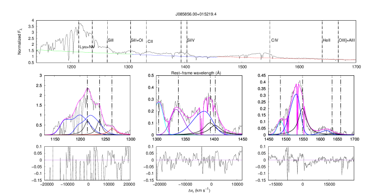
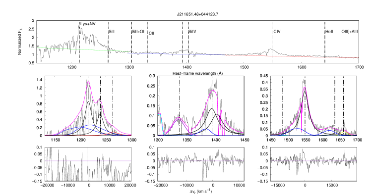
Figure 14: Analysis of sources showing the Ly$\alpha$ + Nv blend. Top: calibrated rest-frame spectrum of SDSS J085856.00+015219.4 (catalog ). before continuum subtraction. Global or local continuum are specified by a continuous coloured line, while the black line mark rest-framed data. Dot-dashed vertical lines correspond to the rest-frame wavelength of each emission line. Bottom: multicomponent fits after continuum subtraction for the L$\alpha\lambda$1216, SiIV$\lambda$1397 and CIV$\lambda$1549 spectral ranges. The continuous black line marks the broad component at rest-frame associated to Ly$\alpha\lambda$1216, NV$\lambda$1240, SiIV$\lambda$1397 and CIV$\lambda$1549. The blue one marks the blueshifted component associated to each emission. The magenta line correspond to the fit to the whole spectrum. In the left bottom panel, the red line corresponds to SiII$\lambda$1265. In the middle bottom panel, the light blue line marks the contribution of OI + SiII$\lambda$1304 blend, while the violet line corresponds to the CII$\lambda$1335 emission line. In the CIV$\lambda$1549 region, NIV]$\lambda$1486 is represented by a light blue line, while the gold one corresponds to the OIII]$\lambda$1663 + AlII$\lambda$1670 blend. Lower panels correspond to the residuals, in radial velocity units km s^-1 and in Å. Bottom: Same as in the previous panels, for SDSS J211651.48+044123.7.

5.4 Role of column density

The column density assumed in the present paper is $\log$$N_{\rm c}$=$23$ [cm^-2]. With this value the emitting clouds in the low-ionization conditions remain optically thick to the Lyman continuum for most of the geometrical depth of the cloud. Even if the value $\log$$N_{\rm c}$=$23$ may appear as a lower limit for the low-ionization BLR, as higher values are required to explain low-ionization emission such as Caii and Feii (Panda, 2020; Panda et al., 2020a), the emission of the intermediate and high-ionized region is confined within the fully ionized part of the line emitting gas whose extension is already much less than the geometrical depth of the gas slab for $\log$$N_{\rm c}$=$23$. Therefore, we expect no or negligible effect from an increase in the column density for the low ionization part of the BLR.

For BLUE, the situation is radically different, and we have no actual strong constraints on column density. Most emission may come from a clumpy outflow (Matthews, 2016, and references therein), and therefore assuming a constant $N_{\rm c}$ may not be appropriate. Considering the poor constrain that we are able to obtain, we leave the issue to an eventual investigation.

5.5 Role of turbulence

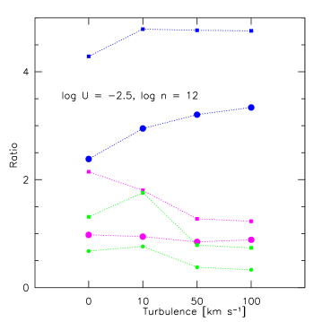
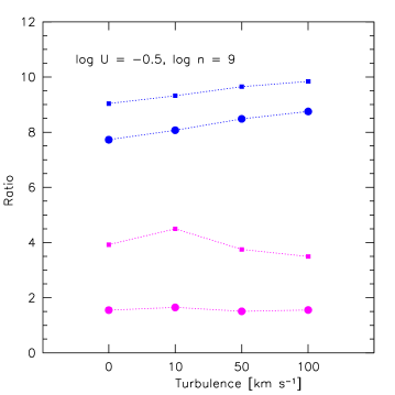
Figure 15: Effects of turbulence on diagnostic line ratios, for Civ/Heii$\lambda$1640 (blue) and Siiv/Heii$\lambda$1640(magenta), considering 5 (circles) and 20 $Z\odot$ (squares), according to CLOUDY 13.05 computations. The top panel assumes the low ionization conditions appropriate for BC emission, the bottom one for BLUE. In the top panel the green lines trace the same trends for the FeII blend at $\lambda 4570$ over H$\beta$ ratio i.e., $R_{\mathrm{FeII}}$.

The results presented in this work refer to the case in which there is no significant micro turbulence included in the CLOUDY computations. Fig. 15 shows that at low ionization the effect is relatively modest, and that in the high-ionization case appropriate for BLUE the effect is very modest. Less obvious is the behavior at low-ionization for $R_{\mathrm{FeII}}$: it shows an increase for $t=10$ km s^-1, but then it has a surprising drop at larger value of the micro-turbulence. While the increase can be explained by an increase of the transitions for which fluorescence is possible, the decrease is not of obvious interpretation. It has been however confirmed by the independent set of simulation of Panda et al. (2018, 2019).

5.6 Metal segregation?

Metals are expected to be preferentially accelerated by resonance scattering (e.g., Proga, 2007b; Risaliti & Elvis, 2010). In principle, for a sufficiently large photon flux, the acceleration of metals by radiation pressure might become larger than the Coulomb friction, therefore causing a decoupling of the metals with respect to their parent plasma (Baskin & Laor, 2012). This possibility has been explored in the context of the BALs, and broad absorption and emission components are expected to be related (Elvis, 2000; Xu et al., 2020). The ionization parameter values are however several orders of magnitudes higher than the ones derived for the BLUE emission component. In addition our $Z$ estimates for the BLUE suggest, if anything, values lower or equal than for the BC, whose $Z$ might be related more to the original chemical composition of the gas in the accretion material. However, we ascribe the systematic differences between BC and BLUE as uncertainties in the method and measurement, so that $Z$ from BLUE and BC should be considered intrinsically equal.

Considering that the most metal rich stars, galaxies, and molecular clouds in the Universe do not exceed $Z\approx 5Z_{\odot}$ (Maiolino & Mannucci, 2019), circumnuclear star formation is needed for the chemical enrichment of the BLR gas (e.g., Collin & Zahn, 1999a, b; Wang et al., 2011, 2012b). Star formation may occur in the self gravitating, outer part of the disk. An alternative possibility is that a massive star could be formed inside the disk by accretion of disk gas (Cantiello et al., 2020).

5.7 Abundance pollution?

An implication of the scenarios involving circumnuclear or even nuclear star formation is that there could be an alteration of the relative abundance of elements with respect to the standard solar composition (Anders & Grevesse, 1989; Grevesse & Sauval, 1998). Support for this hypothesis is provided by the extreme Civ/Siiv and Civ/Aliii that may hint to a selective enhancement of Al with respect to C. As suggested by Negrete et al. (2012), core-collapse supernovæ with very massive progenitors could be at the origin of a selective enhancement. Supernovae with progenitors of masses between 15 and 40 $M_{\odot}$ have selective enhancement in their yields of Al and Si by factors of $\approx$ 100 and 10 relative to Hydrogen with respect to solar (Chieffi & Limongi, 2013). Since Carbon is also increased by a factor $\sim$10 with respect to solar, the [Al/C] is expected to be a factor $\sim 10$ the solar value in supernova ejecta. The case for Silicon is less clear, as the enhancement is of the same order of magnitude of the one expected for Carbon. Pollution of gas by supernovæ may therefore lead to an estimate of the $Z$ higher than the actual one, if solar relative abundances are assumed. This possibility will be explored in an eventual work (Garnica et al., in preparation).

5.8 Implications for quasar structure evolution

Metallicity and the outflow prominence of quasars were found to be highly correlated (Wang et al., 2012a; Shin et al., 2017). The implication of these results is that xA sources, which show the highest blueshifts (Sulentic et al., 2017; Vietri et al., 2018; Martinez-Aldama et al., 2018; Martínez-Aldama et al., 2018), should also be the most metal rich. The xA sources should be at the top of the $Z$ outflow parameter correlation of Wang et al. (2012a), if $Z\gtrsim 10Z_{\odot}$.

There is evidence of a metallicity correlation between BLR and NLR (Du et al., 2014), as expected if the outflows on spatial scales of kpc are originating in a disk wind. Zamanov et al. (2002) derived very small spatial scales at low luminosity. This provides additional support to the idea that xA sources – which at low-$z$ phenomenologically appear as Feii-strong NLSy1s, are relatively young sources. Their low [Oiii]$\lambda$5007 equivalent width implied young age more than orientation effects (Risaliti et al., 2011; Bisogni et al., 2017). The $z\approx 2$ quasars of the present sample are radiating at relatively high $L/L_{\rm Edd}$ although there are no examples of the extremes of xA sources showing blueshifted emission in Aliii as prominent as the one of Civ (e.g., Martínez-Aldama et al., 2017). There is no evidence of heavy obscuration. They are certainly out of the obscured early evolution stage in which the accreting black hole is enveloped by gas and dust (see the sketch in D’Onofrio & Marziani 2018). The $W$ Civ distribution covers the upper half of the one of Martínez-Aldama et al. (2018). There are no weak-lined quasars following Diamond-Stanic et al. (2009). The xA sources of the present sample may have reached a sort of stable equilibrium between gravitation and radiation forces made perhaps possible by the development by an optically thick, geometrically thick accretion disk, and by its anisotropic radiation properties (e.g., Abramowicz et al., 1988; Szuszkiewicz et al., 1996; Sa̧dowski et al., 2014).

The median value of the peak displacement of the BLUE component is around $\approx 3500$ km s^-1, and the centroid at half maximum is shifted by 5000 km s^-1. The extreme blueshifts in the metal lines imply outflows that may not remain bound to the potential well of the black hole and of the inner bulge of the host galaxies (e.g., Marziani et al., 2016b, and references therein). The high metal content of the outflows, estimated by the present work to be in the range $10-50Z_{\odot}$, implies that these sources are likely to be a major source of metal enrichment of the interstellar gas of the host galaxy and of the intergalactic medium. Using a standard estimate for the mass outflow rate $\dot{M}$ (Marziani et al., 2016b), $\dot{M}\approx 15L_{\mathrm{CIV,45}}v_{5000}r_{\mathrm{1pc}}^{-1}n_{9}^{-1}$ $M_{\odot}$ yr^-1, we obtain an outflow rate of $\dot{M}\approx 20M_{\odot}$ yr^-1, assuming median values for the sources of our sample: median outflow velocity from the peak of BLUE $\approx-3500$ km s^-1, a median luminosity of the Civ BLUE (corrected because of Galactic extinction) of 4.2$\cdot$ 10⁴⁴ erg s^-1, a median radius 5.9 $\cdot$ 10¹⁷ cm from the Kaspi et al. (2007) radius-luminosity correlation for Civ, and $n_{9}=1$. For a duty cycle of $\sim 10^{8}$ yr, the expelled mass of heavily enriched-gas could be $\sim 10^{9}M_{\odot}$.

6 Conclusion

The sources at the extreme end of Population A along the main sequence are defined by the prominence of their Feii emission and, precisely, by the selection criterion $R_{\mathrm{FeII}}$$\gtrsim 1$ (Marziani & Sulentic, 2014; Du et al., 2016b). Their properties as a class are scarcely known. Even if there has been a long history of studies focused on Feii-strong sources since Lipari et al. (1993); Graham et al. (1996), their relevance to galactic and large scale structure evolution is being reconsidered anew with the help of the quasar main sequence. This paper adds to other aspects that were considered by previous investigations (for example, the very powerful outflows, the disjoint low- and high-ionization emitting regions, first suggested by Collin-Souffrin et al. 1988), a quantitive analysis of the chemical composition of xA sources. The main aspects of the present investigations can be summarized as follows:

• We distinguish between two emission line components most likely origination from emitting in widely different physical conditions: a virialized low-ionization BLR, and a high-ionization region associated to a very strong blueshifted excess in the Civ emission line. This is the conditio sine qua non for meaningful $Z$ estimates.

• The physical conditions in the low and high regions were confirmed to be very different, with the low ionization ($U$, $n_{\mathrm{H}}$) $\approx$(-2.75, 12.5 – 14) and the high ionization ($U$, $n_{\mathrm{H}}$) $\approx$(-0.5, 8). The high ionization region parameters are however poorly constrained.

• Using intensity ratios between the strongest metal lines and Heii$\lambda$1640 emission at $\lambda 1640$ we derive metallicity values in the range $10\lesssim Z\lesssim 50Z_{\odot}$, with most likely values around several tens of the time solar metallicity. Incidentally, we note that the low equivalent width is consistent the high $Z$ of the emitting regions.

• We find evidence of overabundance of Al with respect to C. This result points toward possible pollution of the broad line emitting gas chemical composition by supernova ejecta.

xA quasars are perhaps the only quasars whose ejection are able to overcome the potential well of the black hole and of the host galaxy. Applying the method to large samples of quasars would permit to constrain the metal enrichment processes on a galactic scale.

The present analysis relied heavily on the Heii$\lambda$1640 line which is of low equivalent width and with a flat, very broad profile. Therefore, a more precise analysis would require spectra of moderate dispersion but of higher S/N ratio. A large part of the scatter and/or systematic difference for various $Z$ estimators is related to the difficulty to isolate faint and broad emission in relatively noisy spectra.

Appendix A Rest-frame spectra and fits

The spectral analysis of the 13 objects of our sample is shown in the figures below.

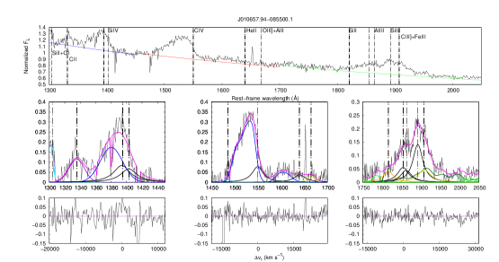
Figure 16: Top panels: calibrated rest-frame spectrum of SDSS J010657.94-085500.1 before continuum substraction. Global or local continuum are specified by a continuous coloured line, while the black line mark rest-framed data. Dot-dashed vertical lines correspond to the rest-frame wavelength of each emission line. Bottom: multicomponent fits after continuum subtraction for the SiIV$\lambda$1397, CIV$\lambda$1549 and $\lambda$1900 blend spectral ranges. The continuous black line marks the broad component at rest-frame associated to SiIV$\lambda$1397, CIV$\lambda$1549 and AlIII$\lambda$1860, the blue one marks the blueshifted component associated to each emission. The magenta line correspond to the fit to the whole spectrum. In the left bottom panel, the light blue line marks the contribution of OI + SII$\lambda$1304 blend, while the violet line corresponds to the CII$\lambda$1335 emission line. In the CIV$\lambda$1549 region, NIV]$\lambda$1486 is represented by a light blue line, while the gold one corresponds to the OIII]$\lambda$1663 + AlII$\lambda$1670 blend. In the $\lambda$1900 blend range, FeIII and FeII contributions are marked dark and light green lines respectively. Violet lines mark the NIII]$\lambda$1750, the orange one corresponds to the SIII$\lambda$1816 and the gold one to the CIII]$\lambda$1909 line. Lower panels correspond to the residuals, in radial velocity units km s^-1 and in Å.

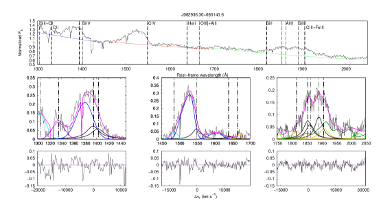
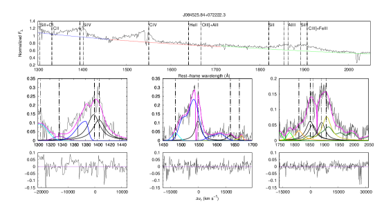
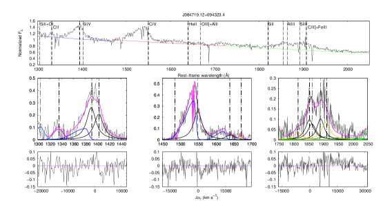
Figure 16: Same of the previous panel, for SDSS J082936.30+080140.6 and SDSS J084525.84+072222.3, and SDSS J084719.12+094323.4.

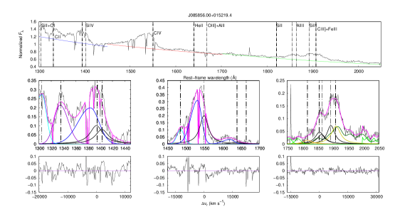
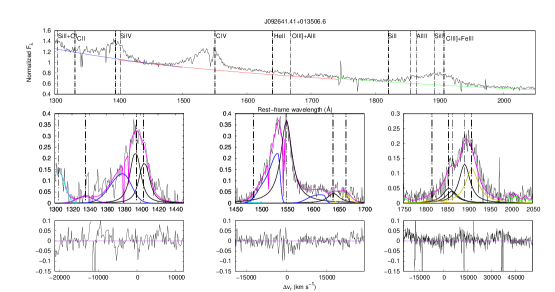
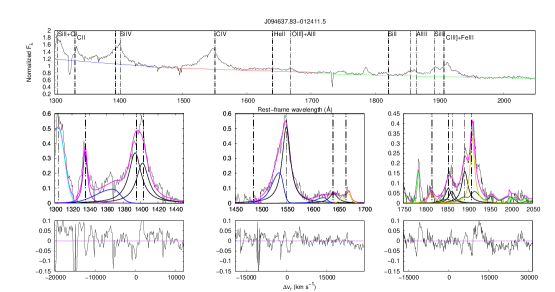
Figure 16: Same of the previous panel, for SDSS J085856.00+015219.4, SDSS J092641.41+013506.6, and SDSS J094637.83-012411.5.

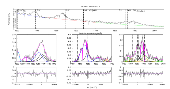
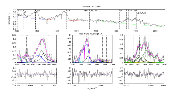
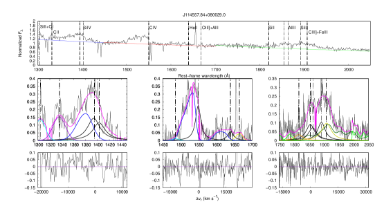
Figure 16: Same of the previous panel, for SDSS J102421.32+024520.2 SDSS J102606.67+011459.0 SDSS J114557.84+080029.0.

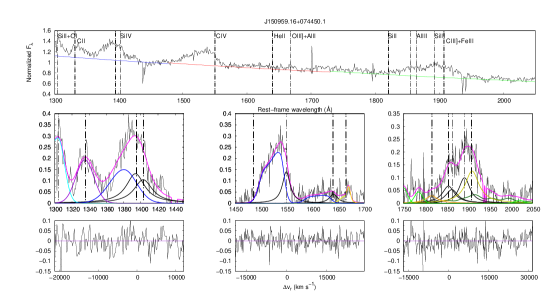
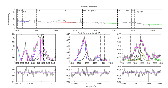
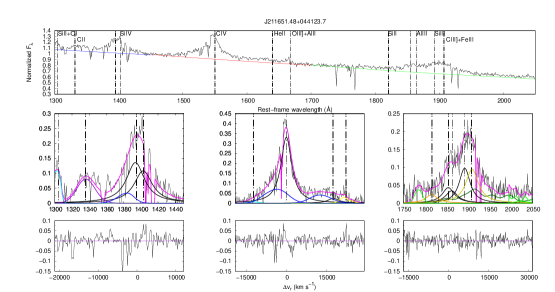
Figure 16: Same of the previous panel, for SDSS J150959.16+074450.1, SDSS J151929.45+072328.7, SDSS J211651.48+044123.7.

Appendix B Diagnostic intensity ratios in the plane ($U$, $n_{\mathrm{H}}$) as a function of metallicity

The results of the arrays of simulations as a function of $n_{\mathrm{H}}$, $U$, and $Z$ are shown below, for $N_{\rm c}$$=10^{23}$. The SED shape is the same for all simulations (table$\_$agn) which corresponds to the SED of Mathews & Ferland (1987). No turbulence was assumed.

References

- Abramowicz et al. (1988) Abramowicz, M. A., Czerny, B., Lasota, J. P., & Szuszkiewicz, E. 1988, ApJ, 332, 646
- Adelman-McCarthy et al. (2008a) Adelman-McCarthy, J. K., Agüeros, M. A., Allam, S. S., et al. 2008a, ApJS, 175, 297
- Adelman-McCarthy et al. (2008b) —. 2008b, ApJS, 175, 297
- Adhikari et al. (2016) Adhikari, T. P., Różańska, A., Czerny, B., Hryniewicz, K., & Ferland, G. J. 2016, ApJ, 831, 68
- Anders & Grevesse (1989) Anders, E., & Grevesse, N. 1989, Geochim. Cosmochim. Acta, 53, 197
- Bañados et al. (2016) Bañados, E., Venemans, B. P., Decarli, R., et al. 2016, ApJS, 227, 11
- Baldwin et al. (2003) Baldwin, J. A., Hamann, F., Korista, K. T., et al. 2003, ApJ, 583, 649
- Baskin & Laor (2012) Baskin, A., & Laor, A. 2012, MNRAS, 426, 1144
- Becker et al. (1995) Becker, R. H., White, R. L., & Helfand, D. J. 1995, ApJ, 450, 559
- Bevington & Robinson (2003) Bevington, P. R., & Robinson, D. K. 2003, Data reduction and error analysis for the physical sciences
- Bisogni et al. (2017) Bisogni, S., di Serego Alighieri, S., Goldoni, P., et al. 2017, A&A, 603, A1
- Boroson & Green (1992) Boroson, T. A., & Green, R. F. 1992, ApJS, 80, 109
- Brotherton et al. (1994) Brotherton, M. S., Wills, B. J., Francis, P. J., & Steidel, C. C. 1994, ApJ, 430, 495
- Brühweiler & Verner (2008) Brühweiler, F., & Verner, E. 2008, ApJ, 675, 83
- Cantiello et al. (2020) Cantiello, M., Jermyn, A. S., & Lin, D. N. C. 2020, arXiv e-prints, arXiv:2009.03936
- Chieffi & Limongi (2013) Chieffi, A., & Limongi, M. 2013, ApJ, 764, 21
- Coatman et al. (2016) Coatman, L., Hewett, P. C., Banerji, M., & Richards, G. T. 2016, MNRAS, 461, 647
- Collin & Zahn (1999a) Collin, S., & Zahn, J.-P. 1999a, A&Ap, 344, 433
- Collin & Zahn (1999b) —. 1999b, Ap&SS, 265, 501
- Collin-Souffrin et al. (1988) Collin-Souffrin, S., Dyson, J. E., McDowell, J. C., & Perry, J. J. 1988, MNRAS, 232, 539
- Collin-Souffrin & Lasota (1988) Collin-Souffrin, S., & Lasota, J.-P. 1988, PASP, 100, 1041
- Corbin & Boroson (1996) Corbin, M. R., & Boroson, T. A. 1996, ApJS, 107, 69
- D’ Agostini (2003) D’ Agostini, G. 2003, Bayesian reasoning in data analysis - A critical introduction (Singapore: World Scientific Co.)
- Davidson & Netzer (1979) Davidson, K., & Netzer, H. 1979, Reviews of Modern Physics, 51, 715
- Diamond-Stanic et al. (2009) Diamond-Stanic, A. M., Fan, X., Brandt, W. N., et al. 2009, ApJ, 699, 782
- Dietrich et al. (2003) Dietrich, M., Hamann, F., Shields, J. C., et al. 2003, ApJ, 589, 722
- D’Onofrio & Marziani (2018) D’Onofrio, M., & Marziani, P. 2018, Frontiers in Astronomy and Space Sciences, 5, 31
- Du et al. (2016a) Du, P., Wang, J.-M., Hu, C., et al. 2016a, ApJ, 818, L14
- Du et al. (2014) —. 2014, MNRAS, 438, 2828
- Du et al. (2016b) Du, P., Lu, K.-X., Hu, C., et al. 2016b, ApJ, 820, 27
- Elvis (2000) Elvis, M. 2000, ApJ, 545, 63
- Feibelman & Aller (1987) Feibelman, W. A., & Aller, L. H. 1987, ApJ, 319, 407
- Ferland et al. (2020) Ferland, G. J., Done, C., Jin, C., Landt, H., & Ward, M. J. 2020, MNRAS, 494, 5917
- Ferland et al. (2009) Ferland, G. J., Hu, C., Wang, J., et al. 2009, ApJ, 707, L82
- Ferland et al. (2013) Ferland, G. J., Porter, R. L., van Hoof, P. A. M., et al. 2013, RevMexA&Ap, 49, 137
- Ferland et al. (2017) Ferland, G. J., Chatzikos, M., Guzmán, F., et al. 2017, Rev. Mexicana Astron. Astrofis., 53, 385
- Gaskell (2000) Gaskell, C. M. 2000, New A Rev., 44, 563
- Graham et al. (1996) Graham, M. J., Clowes, R. G., & Campusano, L. E. 1996, MNRAS, 279, 1349
- Grevesse & Sauval (1998) Grevesse, N., & Sauval, A. J. 1998, Space Sci. Rev., 85, 161
- Hamann & Ferland (1992) Hamann, F., & Ferland, G. 1992, ApJ, 391, L53
- Hamann & Ferland (1999) —. 1999, ARA&A, 37, 487
- Hamann et al. (2002) Hamann, F., Korista, K. T., Ferland, G. J., Warner, C., & Baldwin, J. 2002, ApJ, 564, 592
- Hartig & Baldwin (1986) Hartig, G. F., & Baldwin, J. A. 1986, ApJ, 302, 64
- Izotov & Thuan (1999) Izotov, Y. I., & Thuan, T. X. 1999, ApJ, 511, 639
- Juarez et al. (2009) Juarez, Y., Maiolino, R., Mujica, R., et al. 2009, A&Ap, 494, L25
- Kaspi et al. (2007) Kaspi, S., Brandt, W. N., Maoz, D., et al. 2007, ApJ, 659, 997
- Keenan et al. (2002) Keenan, F. P., Ahmed, S., Brage, T., et al. 2002, MNRAS, 337, 901
- Kovačević-Dojčinović & Popović (2015) Kovačević-Dojčinović, J., & Popović, L. Č. 2015, ApJS, 221, 35
- Kriss (1994) Kriss, G. 1994, Astronomical Data Analysis Software and Systems III, A.S.P. Conference Series, 61, 437
- Kuraszkiewicz et al. (2009) Kuraszkiewicz, J., Wilkes, B. J., Schmidt, G., et al. 2009, ApJ, 692, 1180
- Leighly & Moore (2004) Leighly, K. M., & Moore, J. R. 2004, ApJ, 611, 107
- Lipari et al. (1993) Lipari, S., Terlevich, R., & Macchetto, F. 1993, ApJ, 406, 451
- Maiolino & Mannucci (2019) Maiolino, R., & Mannucci, F. 2019, A&A Rev., 27, 3
- Martínez-Aldama et al. (2017) Martínez-Aldama, M. L., Del Olmo, A., Marziani, P., et al. 2017, Frontiers in Astronomy and Space Sciences, 4, 29
- Martínez-Aldama et al. (2018) Martínez-Aldama, M. L., del Olmo, A., Marziani, P., et al. 2018, A&A, 618, A179
- Martinez-Aldama et al. (2018) Martinez-Aldama, M. L., Del Olmo, A., Marziani, P., et al. 2018, Frontiers in Astronomy and Space Sciences, 4, 65
- Marziani et al. (2020) Marziani, P., del Olmo, A., Perea, J., D’Onofrio, M., & Panda, S. 2020, Atoms, 8, 94
- Marziani et al. (2016a) Marziani, P., Martínez Carballo, M. A., Sulentic, J. W., et al. 2016a, Ap&SS, 361, 29
- Marziani & Sulentic (2014) Marziani, P., & Sulentic, J. W. 2014, MNRAS, 442, 1211
- Marziani et al. (1996) Marziani, P., Sulentic, J. W., Dultzin-Hacyan, D., Calvani, M., & Moles, M. 1996, ApJS, 104, 37
- Marziani et al. (2010) Marziani, P., Sulentic, J. W., Negrete, C. A., et al. 2010, MNRAS, 409, 1033
- Marziani et al. (2016b) Marziani, P., Sulentic, J. W., Stirpe, G. M., et al. 2016b, Ap&SS, 361, 3
- Marziani et al. (2009) Marziani, P., Sulentic, J. W., Stirpe, G. M., Zamfir, S., & Calvani, M. 2009, A&Ap, 495, 83
- Marziani et al. (2018) Marziani, P., Dultzin, D., Sulentic, J. W., et al. 2018, Frontiers in Astronomy and Space Sciences, 5, 6
- Mathews & Ferland (1987) Mathews, W. G., & Ferland, G. J. 1987, ApJ, 323, 456
- Mathur (2000) Mathur, S. 2000, MNRAS, 314, L17
- Matsuoka et al. (2011) Matsuoka, K., Nagao, T., Marconi, A., Maiolino, R., & Taniguchi, Y. 2011, A&A, 527, A100
- Matsuoka et al. (2007) Matsuoka, Y., Oyabu, S., Tsuzuki, Y., & Kawara, K. 2007, ApJ, 663, 781
- Matthews (2016) Matthews, J. H. 2016, PhD thesis, University of Southampton
- Mejía-Restrepo et al. (2016) Mejía-Restrepo, J. E., Trakhtenbrot, B., Lira, P., Netzer, H., & Capellupo, D. M. 2016, MNRAS, 460, arXiv:1603.03437
- Murray & Chiang (1997) Murray, N., & Chiang, J. 1997, ApJ, 474, 91
- Murray et al. (1995) Murray, N., Chiang, J., Grossman, S. A., & Voit, G. M. 1995, ApJ, 451, 498
- Nagao et al. (2006a) Nagao, T., Maiolino, R., & Marconi, A. 2006a, A&A, 447, 863
- Nagao et al. (2006b) Nagao, T., Marconi, A., & Maiolino, R. 2006b, A&Ap, 447, 157
- Nardini et al. (2019) Nardini, E., Lusso, E., Risaliti, G., et al. 2019, A&A, 632, A109
- Negrete et al. (2012) Negrete, A., Dultzin, D., Marziani, P., & Sulentic, J. 2012, ApJ, 757, 62
- Negrete et al. (2010) Negrete, C. A., Dultzin, D., Marziani, P., & Sulentic, J. 2010, ArXiv e-prints, arXiv:1011.4248
- Negrete et al. (2014) Negrete, C. A., Dultzin, D., Marziani, P., & Sulentic, J. W. 2014, ApJ, 794, 95
- Negrete et al. (2018) Negrete, C. A., Dultzin, D., Marziani, P., et al. 2018, A&A, 620, A118
- Netzer & Marziani (2010) Netzer, H., & Marziani, P. 2010, ApJ, 724, 318
- Onoue et al. (2020) Onoue, M., Bañados, E., Mazzucchelli, C., et al. 2020, ApJ, 898, 105
- Osmer & Smith (1976) Osmer, P. S., & Smith, M. G. 1976, ApJ, 210, 267
- Osterbrock & Ferland (2006) Osterbrock, D. E., & Ferland, G. J. 2006, Astrophysics of gaseous nebulae and active galactic nuclei (Mill Valley, CA: University Science Books)
- Osterbrock & Pogge (1985) Osterbrock, D. E., & Pogge, R. W. 1985, ApJ, 297, 166
- Panda (2020) Panda, S. 2020, arXiv e-prints, arXiv:2004.13113
- Panda et al. (2018) Panda, S., Czerny, B., Adhikari, T. P., et al. 2018, ApJ, 866, 115
- Panda et al. (2020a) Panda, S., Martínez-Aldama, M. L., Marinello, M., et al. 2020a, ApJ, 902, 76
- Panda et al. (2019) Panda, S., Marziani, P., & Czerny, B. 2019, ApJ, 882, 79
- Panda et al. (2020b) —. 2020b, Contributions of the Astronomical Observatory Skalnate Pleso, 50, 293
- Pâris et al. (2017) Pâris, I., Petitjean, P., Ross, N. P., et al. 2017, A&A, 597, A79
- Peimbert et al. (2001) Peimbert, A., Peimbert, M., & Luridiana, V. 2001, in Revista Mexicana de Astronomia y Astrofisica Conference Series, Vol. 10, Revista Mexicana de Astronomia y Astrofisica Conference Series, ed. J. Cantó & L. F. Rodríguez, 148–153
- Peimbert (2008) Peimbert, M. 2008, arXiv e-prints, arXiv:0811.2980
- Peterson & Wandel (1999) Peterson, B. M., & Wandel, A. 1999, ApJ, 521, L95
- Plotkin et al. (2015) Plotkin, R. M., Shemmer, O., Trakhtenbrot, B., et al. 2015, ApJ, 805, 123
- Popović et al. (2002) Popović, L. Č., Mediavilla, E. G., Kubičela, A., & Jovanović, P. 2002, A&A, 390, 473
- Proga (2007a) Proga, D. 2007a, ApJ, 661, 693
- Proga (2007b) Proga, D. 2007b, in Astronomical Society of the Pacific Conference Series, Vol. 373, The Central Engine of Active Galactic Nuclei, ed. L. C. Ho & J.-W. Wang, 267
- Punsly et al. (2018) Punsly, B., Marziani, P., Bennert, V. N., Nagai, H., & Gurwell, M. A. 2018, ApJ, 869, 143
- Richards et al. (2006) Richards, G. T., Lacy, M., Storrie-Lombardi, L. J., et al. 2006, ApJS, 166, 470
- Richards et al. (2011) Richards, G. T., Kruczek, N. E., Gallagher, S. C., et al. 2011, AJ, 141, 167
- Risaliti & Elvis (2010) Risaliti, G., & Elvis, M. 2010, A&A, 516, A89
- Risaliti et al. (2011) Risaliti, G., Salvati, M., & Marconi, A. 2011, MNRAS, 411, 2223
- Sa̧dowski et al. (2014) Sa̧dowski, A., Narayan, R., McKinney, J. C., & Tchekhovskoy, A. 2014, MNRAS, 439, 503
- Schneider et al. (2010) Schneider, D. P., Richards, G. T., Hall, P. B., et al. 2010, AJ, 139, 2360
- Shemmer & Netzer (2002) Shemmer, O., & Netzer, H. 2002, ApJ, 567, L19
- Shemmer et al. (2004) Shemmer, O., Netzer, H., Maiolino, R., et al. 2004, ApJ, 614, 547
- Shen (2016) Shen, Y. 2016, ApJ, 817, 55
- Shen & Ho (2014) Shen, Y., & Ho, L. C. 2014, Nature, 513, 210
- Shen et al. (2011) Shen, Y., Richards, G. T., Strauss, M. A., et al. 2011, ApJS, 194, 45
- Shields (1976) Shields, G. A. 1976, ApJ, 204, 330
- Shin et al. (2017) Shin, J., Nagao, T., & Woo, J.-H. 2017, ApJ, 835, 24
- Shin et al. (2013) Shin, J., Woo, J.-H., Nagao, T., & Kim, S. C. 2013, ApJ, 763, 58
- Sulentic et al. (2007) Sulentic, J. W., Bachev, R., Marziani, P., Negrete, C. A., & Dultzin, D. 2007, ApJ, 666, 757
- Sulentic et al. (2014) Sulentic, J. W., Marziani, P., del Olmo, A., et al. 2014, A&A, 570, A96
- Sulentic et al. (2000a) Sulentic, J. W., Marziani, P., & Dultzin-Hacyan, D. 2000a, ARA&A, 38, 521
- Sulentic et al. (1995) Sulentic, J. W., Marziani, P., Dultzin-Hacyan, D., Calvani, M., & Moles, M. 1995, ApJL, 445, L85
- Sulentic et al. (2002) Sulentic, J. W., Marziani, P., Zamanov, R., et al. 2002, ApJL, 566, L71
- Sulentic et al. (2006) Sulentic, J. W., Repetto, P., Stirpe, G. M., et al. 2006, A&Ap, 456, 929
- Sulentic et al. (2000b) Sulentic, J. W., Zwitter, T., Marziani, P., & Dultzin-Hacyan, D. 2000b, ApJL, 536, L5
- Sulentic et al. (2017) Sulentic, J. W., del Olmo, A., Marziani, P., et al. 2017, A&A, 608, A122
- Szuszkiewicz et al. (1996) Szuszkiewicz, E., Malkan, M. A., & Abramowicz, M. A. 1996, ApJ, 458, 474
- Temple et al. (2020) Temple, M. J., Ferland, G. J., Rankine, A. L., et al. 2020, MNRAS, 496, 2565
- Vanden Berk et al. (2001) Vanden Berk, D. E., Richards, G. T., Bauer, A., et al. 2001, AJ, 122, 549
- Verner et al. (1999) Verner, E. M., Verner, D. A., Korista, K. T., et al. 1999, ApJS, 120, 101
- Véron-Cetty et al. (2001) Véron-Cetty, M.-P., Véron, P., & Gonçalves, A. C. 2001, AAp, 372, 730
- Vestergaard & Peterson (2006) Vestergaard, M., & Peterson, B. M. 2006, ApJ, 641, 689
- Vestergaard & Wilkes (2001) Vestergaard, M., & Wilkes, B. J. 2001, ApJS, 134, 1
- Vietri et al. (2018) Vietri, G., Piconcelli, E., Bischetti, M., et al. 2018, A&A, 617, A81
- Vila-Costas & Edmunds (1993) Vila-Costas, M. B., & Edmunds, M. G. 1993, MNRAS, 265, 199
- Wang et al. (2012a) Wang, H., Zhou, H., Yuan, W., & Wang, T. 2012a, ApJ, 751, L23
- Wang et al. (2012b) Wang, J.-M., Du, P., Baldwin, J. A., et al. 2012b, ApJ, 746, 137
- Wang et al. (2014) Wang, J.-M., Du, P., Li, Y.-R., et al. 2014, ApJ, 792, L13
- Wang et al. (2013) Wang, J.-M., Du, P., Valls-Gabaud, D., Hu, C., & Netzer, H. 2013, Physical Review Letters, 110, 081301
- Wang et al. (2011) Wang, J.-M., Ge, J.-Q., Hu, C., et al. 2011, ApJ, 739, 3
- Warner et al. (2004) Warner, C., Hamann, F., & Dietrich, M. 2004, ApJ, 608, 136
- Welch (1947) Welch, B. L. 1947, Biometrika, 34, 28
- Wildy et al. (2019) Wildy, C., Czerny, B., & Panda, S. 2019, A&A, 632, A41
- Wills & Netzer (1979) Wills, D., & Netzer, H. 1979, ApJ, 233, 1
- Xu et al. (2012) Xu, D., Komossa, S., Zhou, H., et al. 2012, AJ, 143, 83
- Xu et al. (2020) Xu, X., Zakamska, N. L., Arav, N., Miller, T., & Benn, C. 2020, MNRAS, 495, 305
- Zamanov et al. (2002) Zamanov, R., Marziani, P., Sulentic, J. W., et al. 2002, ApJL, 576, L9
- Zheng (1988) Zheng, W. 1988, Astrophysical Letters and Communications, 27, 275
- Zhou et al. (2006) Zhou, H., Wang, T., Yuan, W., et al. 2006, ApJS, 166, 128