Sigma-Eight at the Percent Level: The EFT Likelihood in Real Space

Abstract

The effective field theory likelihood for the density field of biased tracers allows for cosmology inference from the clustering of galaxies that consistently uses all available information at a given order in perturbation theory. This paper presents results and implementation details on the real-space (as opposed to Fourier-space) formulation of the likelihood, which allows for the incorporation of survey window functions. The implementation further uses a Lagrangian forward model for biased tracers which automatically accounts for all relevant contributions up to any desired order. Unbiased inference of $\sigma_{8}$ is demonstrated at the 2% level for cutoff values $\Lambda\leq 0.14\,h\,\text{Mpc}^{-1}$ for halo samples over a range of masses and redshifts. The inferred value shows the expected convergence to the ground truth in the low-cutoff limit. Apart from the possibility of including observational effects, this represents further substantial improvement over previous results based on the EFT likelihood.

1 Introduction

It is well established that the large-scale clustering of galaxies contains a wealth of information on cosmology. This includes in particular the angular diameter distance $D_{A}(z)$ and expansion rate $H(z)$ inferred from the baryon acoustic oscillation (BAO) feature, the growth rate of structure in form of the parameter combination $f\sigma_{8}$ inferred from redshift-space distortions (RSD), and the amplitude of local-type primordial non-Gaussianity $f_{\rm NL}$ via the large-scale scale-dependent bias. All of these constraints are accessible using linear information, i.e. using linear theory model predictions for the galaxy power spectrum or 2-point correlation function, although nonlinear corrections are important to take into account essentially as theoretical error bar [1, 2, 3].

However, there is significantly more information to be exploited in the nonlinear part of galaxy clustering. An example is BAO reconstruction, which reduces the inferred error bars on $D_{A},H$ by performing a nonlinear operation on the data (e.g., [4, 5]). Another is the normalization of the linear matter power spectrum $\sigma_{\mathrm{8}}$, which at linear order is perfectly degenerate with the linear galaxy bias parameter $b_{1}$ (see Secs. 1-2 of [6] for an introduction to the topic of bias). Including nonlinear information, for example via the bispectrum, allows for this degeneracy to be broken. Combined with RSD, this in turn allows for independent constraints on the growth rate proper $f=d\ln D/d\ln a$ where $D(a)$ is the linear growth factor, and $\sigma_{\mathrm{8}}$, allowing for interesting additional tests of the $\Lambda$CDM paradigm and possibly improved constraints on the sum of neutrino masses. It is also worth noting that selection effects can spoil the determination of $f\sigma_{8}$ at linear order [7, 8, 9, 10, 11, 12, 13], in which case nonlinear information is likewise necessary in order to extract the growth rate [14].

Linear information is by definition optimally extracted via the power spectrum. A new approach to extracting the nonlinear information, which is only marginally accessed by the power spectrum, has recently gathered increased attention: Loosely referred to as forward modeling, this approach proceeds by writing down a likelihood for the entire galaxy density field, and performing a full joint Bayesian inference of cosmological parameters along with the phases of the initial conditions corresponding to the observed survey volume [15, 16, 17, 18, 19, 20, 21, 22, 23, 24, 25, 26, 27, 28, 29, 30, 31, 32]. The crucial ingredient in this inference approach is the conditional probability (“likelihood”) of the observed galaxy density field given the forward-evolved matter density field. Unbiased inference depends very sensitively on the accuracy of the likelihood for the galaxy density field. Refs. [33, 34, 35] recently derived the likelihood in the context of the effective field theory (EFT [36, 37]) of large-scale structure. By including only modes with wavenumbers below a cutoff, or maximum wavenumber $\Lambda$, this allows for a rigorous, controlled Bayesian inference of cosmology and initial conditions, provided that the cutoff is chosen to only include modes for which perturbation theory is valid ($\Lambda\lesssim 0.25\,h\,\text{Mpc}^{-1}$ at $z=0$).

Ref. [38] presented results of the EFT likelihood applied to halo samples in their rest frame (i.e. without RSD) identified in N-body simulations. In particular, unbiased inference of $\sigma_{\mathrm{8}}$ (equivalent, when all remaining cosmological parameters are fixed, to the primordial normalization $\sqrt{\mathcal{A}_{s}}$) was demonstrated at the 4–8% level depending on halo mass and redshift. In this test, the phases of the forward model were fixed to the truth, i.e. the initial conditions used in the N-body simulations. As mentioned above, the constraint on $\sigma_{\mathrm{8}}$ is not obtainable using linear theory due to the bias-amplitude degeneracy, and so is exclusively due to the robust extraction of nonlinear information. These results were based on a Fourier-space formulation of the EFT likelihood.

In this paper, we present an implementation of the EFT likelihood in real space based on [39]. As shown in Ref. [39], this formulation allows for an incorporation of the most important corrections to the leading EFT likelihood, a Gaussian with constant diagonal noise, in particular the modulation of the noise by long-wavelength modes, or equivalently the stochasticity of the bias parameters. Moreover, this formulation also permits one to include the survey window function in a computationally efficient way. We describe how this works in Sec. 2.

We further employ a new Lagrangian forward model to predict the mean galaxy density given fixed phases. This forward model is recursively constructed to any desired order based on Lagrangian perturbation theory (LPT), without assuming the Einstein-de Sitter approximation that is usually adopted. It also includes all or a large fraction of the relevant higher-derivative contributions (depending on order). Apart from the efficient, recursive construction to any order, the Lagrangian forward model has the further advantage of a straightforward transformation to redshift space and the lightcone, i.e. onto the observer’s past lightcone rather than a constant proper time slice. We briefly describe the forward model in Sec. 3, relegating a more detailed exposition to the upcoming Ref. [40].

To summarize, this paper presents an implementation of the EFT likelihood that allows for the efficient incorporation of perturbation theory contributions up to any desired order, as well as the leading observational effects, namely RSD, lightcone, and window function.

In our results, we will again restrict to the $\sigma_{\mathrm{8}}$ inference from rest-frame halo catalogs, deferring the inclusion of RSD, lightcone and window function to upcoming work. Thus, our goal will be to test the convergence of perturbation theory as a function of the cutoff $\Lambda$ at the level of the $\sigma_{\mathrm{8}}$ inference, and the extent to which going to higher order improves the latter. Fig. 5 shows a summary of the results, namely the residual fractional error in $\sigma_{\mathrm{8}}$, $\hat{A}_{\rm in}-1$, for all halo samples and redshifts at a fixed cutoff $\Lambda$ and for different expansion orders.

The paper is organized as follows. In Sec. 2 we present the real-space EFT likelihood, including subtleties such as the implementation of the sharp-$k$ cut, and discuss the incorporation of the window function. Sec. 3 briefly presents the forward model and bias expansion, including the ordering scheme used to determine the relevant higher-derivative and stochastic operators. Sec. 4 presents details on the numerical implementation, including marginalization of the (numerous) bias parameters. We then turn to the results in Sec. 5, and their discussion in Sec. 6. We conclude in Sec. 7. The appendices provide additional figures, and more details on the halo samples and numerical implementation.

2 The EFT likelihood in real space

The goal of the forward-modeling approach to galaxy clustering is to evaluate the posterior $\mathcal{P}(\theta|{\delta}_{g})$ of the cosmological parameters $\theta$ given the observed galaxy density field ${\delta}_{g}(\bm{x})$. This is obtained by marginalizing the likelihood $\mathcal{P}({\delta}_{g}|\theta,\{b_{O}\},{\delta}_{\rm in})$ over the phases ${\delta}_{\rm in}$ corresponding to the primordial fluctuations in the volume covered by the galaxy survey, which are drawn from a multivariate Gaussian prior $\mathcal{P}({\delta}_{\rm in}|\theta)$, as well as nuisance parameters such as the bias coefficients $\{b_{O}\}$. The key physical ingredient in this approach thus is the likelihood $\mathcal{P}({\delta}_{g}|\theta,\{b_{O}\},{\delta}_{\rm in})$. The contribution of [33, 34, 35, 38] was to derive this likelihood in the context of the effective field theory of LSS.

Before turning to the likelihood, let us consider the specific question we will investigate numerically in this paper. The highly nontrivial and numerically costly marginalization over the phases can be avoided by looking at simulations: then we can fix ${\delta}_{\rm in}$ to the known initial density field of the simulations. Further, studying physical tracers (in this case, halos) in their rest frame allows us to drop redshift-space distortions from the forward model. Finally, we restrict the set of cosmological parameters $\theta$ to the linear power spectrum normalization $\sigma_{\mathrm{8}}$; equivalently, the square-root of the primordial amplitude $\sqrt{\mathcal{A}_{s}}$. Thus, the question we investigate below, the same question as considered in [33, 34, 38], is: How well can one recover $\sigma_{\mathrm{8}}$ from a rest-frame tracer catalog, with no prior knowledge on the selection, i.e. bias parameters, but assuming perfect knowledge of the phases of the initial conditions? This question is highly nontrivial, since $\sigma_{\mathrm{8}}$ is perfectly degenerate with the linear bias $b_{1}$ in linear theory (i.e. on large scales). Thus, all constraints obtained in $\sigma_{\mathrm{8}}$ are based purely on nonlinear information.

Let us now turn to the likelihood $\mathcal{P}({\delta}_{g}|\sigma_{\mathrm{8}},\{b_{O}\},{\delta}_{\rm in})$, simply referred to as “likelihood” in the following, which we need for this study. As discussed at length in [33, 34, 35, 38], the likelihood for the density field of a biased tracer ${\delta}_{g}(\bm{x})$ consists of

1. a model for the nonlinear evolution of the matter density under gravity, which we denote as ${\delta}_{\rm fwd}[{\delta}_{\rm in}]$;

2. a deterministic bias expansion of the biased tracer, which we denote as $\delta_{g,\rm det}[{\delta}_{\rm in}]$, and which incorporates ingredient $(i)$; and

3. the log-likelihood $\ln\mathcal{P}({\delta}_{g}|\delta_{g,\rm det})$ for the observed galaxy field, i.e. the data ${\delta}_{g}(\bm{x})$ given the deterministic prediction $\delta_{g,\rm det}$.

Note that $\delta_{g,\rm det}$ depends on a set of bias parameters $b_{O}$ which in general have to be determined from the data. In this section we focus on ingredient $(iii)$, and turn to the bias expansion employed here in Sec. 3.

Refs. [33, 34, 35, 38] were based on an expression for the likelihood given in Fourier space,

$$\ln\mathcal{P}({\delta}_{g}|\delta_{g,\rm det})=-\frac{1}{2}\int_{|\bm{k}|<\Lambda}\frac{d^{3}\bm{k}}{(2\pi)^{3}}\left\{\left[\frac{|{\delta}_{g}(\bm{k})-\delta_{g,\rm det}(\bm{k})|^{2}}{P_{\varepsilon}(k)}+\ln[2\pi P_{\varepsilon}(k)]\right]\right\}$$ (2.1)

where the noise variance is parametrized as

$$P_{\varepsilon}(k)=P_{\varepsilon}^{\{0\}}+P_{\varepsilon}^{\{2\}}k^{2}+\ldots,$$ (2.2)

and $\Lambda$ is the cutoff in wavenumber. If we set the subleading contribution $P_{\varepsilon}^{\{2\}}$, as well as all higher-order terms in the expansion Eq. (2.2), to zero, then Eq. (2.1) can be formally transformed to a real-space likelihood, by way of Parseval’s theorem:

$$\ln\mathcal{P}({\delta}_{g}|\delta_{g,\rm det})\stackrel{{\scriptstyle P_{\varepsilon}={\rm const}}}{{=}}-\frac{1}{2}\int d^{3}\bm{x}\left[\frac{\left({\delta}_{g,\Lambda}(\bm{x})-{\delta}_{g,\rm det,\Lambda}(\bm{x})\right)^{2}}{P_{\varepsilon}^{\{0\}}}\right]-\frac{1}{2}N_{\rm modes}\ln[2\pi P_{\varepsilon}^{\{0\}}]$$ (2.3)

where the fields ${\delta}_{g,\Lambda}$ and ${\delta}_{g,\rm det,\Lambda}$ are sharp-$k$ filtered at the cutoff $\Lambda$, i.e.

$${\delta}_{g,\Lambda}(\bm{k})\equiv{\delta}_{g}(\bm{k})W_{\Lambda}(\bm{k})$$ (2.4)

and similarly for ${\delta}_{g,\rm det,\Lambda}$. The filter choice corresponding to Eq. (2.1) is $W_{\Lambda}(\bm{k})=\Theta_{\text{H}}(\Lambda-|\bm{k}|)$, where $\Theta_{\text{H}}$ is the Heaviside function. $N_{\rm modes}$ is the number of modes that survive the sharp-$k$ cut (hence this number is proportional to the volume), ensuring the equivalence to Eq. (2.1).

A real-space expression for the likelihood offers several advantages. First, as argued in [39], the leading perturbative corrections to the likelihood beyond the constant-noise expression Eq. (2.3) are in fact the modulation of the noise amplitude by long-wavelength perturbations (field-dependent stochasticity) rather than the higher-derivative terms in Eq. (2.2); schematically, these are given in real space by

$$P_{\varepsilon}(\bm{x})=P_{\varepsilon}^{\{0\}}+P_{{\varepsilon},{\varepsilon}_{\delta}}{\delta}(\bm{x})+\ldots.$$ (2.5)

Physically, it is expected that the noise in the tracer field is different in high- vs. low-density regions. This effect is captured by Eq. (2.5). An equivalent interpretation is that it encodes stochasticity in the bias parameters; specifically, the term in Eq. (2.5) corresponds to stochasticity in the linear bias $b_{1}=b_{\delta}$. The reason that the term $\propto{\delta}(\bm{x})$ in Eq. (2.5) is more relevant than the $k^{2}$ term in Eq. (2.2) is the shape of the matter power spectrum, since ${\delta}(\bm{x})\sim[k^{3}P_{\text{L}}(k)/2\pi^{2}]^{1/2}_{k=\Lambda}\propto\Lambda^{(3+n_{\text{L}})/2}$, if the linear matter power spectrum $P_{\text{L}}(k)\propto k^{n_{\text{L}}}$, while the higher-derivative term in Eq. (2.2) scales as $\Lambda^{2}$. For $n_{\text{L}}\approx-1.5$, the former is more relevant.

The second significant advantage of a real-space likelihood is that it allows for a more direct incorporation of the window function of an actual galaxy survey. Consider the simplest case of a binary window function, where $\mathcal{W}(\bm{x})=1$ if the region containing $\bm{x}$ is observed, and $\mathcal{W}(\bm{x})=0$ otherwise (this includes the case where we do not trust the selection of galaxies in a given region e.g. due to flux calibration issues caused by bright nearby stars). In the context of a Bayesian forward model, $\mathcal{W}(\bm{x})=0$ corresponds to setting $P_{\varepsilon}(\bm{x})$ to infinity; thus, we can generalize Eq. (2.3) to include the window function:

$$\ln\mathcal{P}({\delta}_{g}|\delta_{g,\rm det})=-\frac{1}{2}\int_{\mathcal{W}(\bm{x})>0}d^{3}\bm{x}\left[\frac{\left({\delta}_{g}^{\Lambda}(\bm{x})-\delta_{g,\rm det}^{\Lambda}(\bm{x})\right)^{2}}{P_{\varepsilon}^{\{0\}}}\right]+{\cal N}\quad\mbox{(binary window function $\mathcal{W}$)},$$ (2.6)

where ${\cal N}$ is a normalization constant. Notice that, unlike the expansions in Eq. (2.2) and Eq. (2.5), the window function is a non-perturbative effect. We defer an actual implementation of window functions to future work, restricting this paper to simulations with trivial window functions $\mathcal{W}=1$. To summarize, we expect that a real-space likelihood will capture both the dominant observational effect as well as the leading perturbative corrections to the EFT likelihood.

Unfortunately, the actual implementation is not quite as simple as Eq. (2.3). In order to obtain a practical real-space likelihood, we need to satisfy two requirements: a field-level covariance that is diagonal in real space (otherwise, the likelihood would not simply be given by a single integral over real space as in Eq. (2.3)); and a sharp-$k$ filter which ensures that only modes with $|\bm{k}|<\Lambda$ appear in the likelihood. We can think of the second requirement in Fourier space, again specializing to a constant noise covariance $P_{\varepsilon}(k)=P_{\varepsilon}^{\{0\}}$, as a diagonal covariance with a step-function behavior:

$${\rm Cov}(\bm{k},\bm{k}^{\prime})=(2\pi)^{3}\delta_{\mathrm{D}}^{(3)}(\bm{k}+\bm{k}^{\prime})P_{\varepsilon}(k)\Big{|}_{\Lambda}\quad\mbox{where}\quad P_{\varepsilon}(k)\Big{|}_{\Lambda}=\left\{\begin{array}[]{ll}P_{\varepsilon}^{\{0\}},&k<\Lambda\\ \infty,&k\geq\Lambda\end{array}\right..$$ (2.7)

If we transform this covariance into real space, the result is not diagonal [39]. This is in keeping with Parseval’s theorem, since we cannot invoke it to go from Eq. (2.1) to Eq. (2.3) if $P_{\varepsilon}$ is not constant.

An alternative opens up if we move away from the spherical sharp-$k$ cut to a cubic cut,

$$W_{\Lambda}(\bm{k})=\Theta_{\text{H}}(\Lambda-|\bm{k}|)\longrightarrow\prod_{i=1}^{3}\Theta_{\text{H}}(\Lambda-k_{i}),$$ (2.8)

where $k_{i}$ denote the Cartesian components of the Fourier vector $\bm{k}$. Notice that the maximum wavenumber allowed by the cubic filter is $\sqrt{3}\Lambda$. In this case, we can use a discrete Fourier representation of the filtered fields (Eq. (2.4)) which preserves precisely those modes that are nonzero after the cubic sharp-$k$ filter in Eq. (2.8). This is achieved by choosing a grid size $N_{g}$ such that $k_{\rm Ny}(N_{g})/2=\Lambda$, where $k_{\rm Ny}$ is the Nyquist frequency of the grid; that is,

$$N_{g}(\Lambda)=\left\lfloor\frac{L_{\text{box}}\Lambda}{\pi}\right\rfloor,$$ (2.9)

where $L_{\text{box}}$ is the side length of the cubic box in real space. More precisely, we choose the largest even number that is smaller than $L_{\text{box}}\Lambda/\pi$. In the case studied here, $L_{\text{box}}^{3}$ corresponds to the simulation volume, while in an application to real data this would be the reconstruction volume which encompasses the entire survey. Note that Eq. (2.9) restricts the actual cutoff to discrete values; however, if $L_{\text{box}}\Lambda\gg 1$, as is the case in practical applications, this is a minor restriction.

The filter Eq. (2.8) breaks rotational invariance, i.e. it introduces preferred directions. For simulated objects, this is not expected to be an issue, since there are no intrinsic directions in the simulations that the coordinate axes could align with. In the application to real data, it is possible that the alignment of the coordinate axes with preferred directions in the survey volume could lead to small systematic artefacts. This can however be tested for by rotating the coordinate axes of the reconstruction volume.

Once the fields are discretized on a Fourier-space grid of size $N_{g}(\Lambda)$, one can then transform them back to real space to obtain representations, e.g. ${\delta}_{g,\Lambda}(\bm{x})$, which only contain modes below the cutoff. It is then appropriate to use a diagonal, real-space likelihood in terms of ${\delta}_{g,\Lambda}(\bm{x}),{\delta}_{g,\rm det,\Lambda}(\bm{x})$ which can incorporate the field-dependent stochasticity in Eq. (2.5), as well as the window function. The details of the implementation are described in Sec. 4. In this paper, we will restrict to a constant covariance in real space, for reasons discussed in that section.

3 Construction of biased field

The deterministic mean-field prediction for the galaxy density can generally be written as

$$\delta_{g,\rm det}(\bm{x},\tau)=\sum_{O}b_{O}(\tau)O(\bm{x},\tau),$$ (3.1)

where $b_{O}$ denote the bias coefficients, and the operators $O$ are in general constructed from the second-derivative tensor of the gravitational potential, $\partial_{i}\partial_{j}\Phi$, and spatial derivatives thereof. The operators are designed to span the entire set of local gravitational observables, and are ordered in terms of perturbations (powers of $\Phi$) and number of spatial derivatives, so that there is only a finite number of operators relevant at a given order (we will return to the precise ordering in Sec. 3.2). The goal then is to obtain constraints on cosmological parameters after marginalizing over the bias parameters $b_{O}$, which in general are unknown for a given observed LSS tracer (certainly not known to the percent level required for precision inference of cosmological parameters). The same set of operators also appears in the expansion of the real-space covariance, Eq. (2.5).

In this section, we describe the construction of the operators $O(\bm{x})$. The previous papers in this series [33, 34, 38] used a Eulerian bias expansion (but, unlike e.g. [41], built on the LPT matter density). That is, the bias operators were constructed out of the forward-evolved matter density field. Here, we instead use a Lagrangian bias expansion, which first constructs the bias operators and then displaces them to the Eulerian frame. This is very similar to the approach recently described in [31], and has several advantages as mentioned in Sec. 1. We provide an outline here, with more details being presented in the upcoming Ref. [40].

3.1 Lagrangian bias expansion

The Lagrangian density of any biased tracer can be expanded as

$$\delta_{g,\rm det}^{\rm L}(\bm{q},\tau)=\sum_{O}b_{O}^{\rm L}O^{\rm L}(\bm{q},\tau),$$ (3.2)

where a superscript L indicates quantities in the Lagrangian (fluid rest) frame. More precisely, $\bm{q}$ denotes the initial positions of matter particles as $\tau\to 0$. The relation to the final observed position is given by the Lagrangian displacement $\bm{s}$, via

$$\bm{x}(\tau)=\bm{q}+\bm{s}(\bm{q},\tau).$$ (3.3)

Since the density perturbations at the initial time are vanishingly small, the late-time matter density field is completely described by the displacement field $\bm{s}(\bm{q},\tau)$, which can be expanded in orders of perturbations:

$$\bm{s}(\bm{q},\tau)=\bm{s}^{(1)}(\bm{q},\tau)+\bm{s}^{(2)}(\bm{q},\tau)+\cdots.$$ (3.4)

The equations of motion of $\bm{s}$ can be integrated to give convenient recursion relations that allow for a relatively simple numerical computation of the $\bm{s}^{(n)}$ [42, 43, 44, 40].

As argued in [45] (see also Sec. 2.5 of [6]), the set of Lagrangian bias operators $O^{\rm L}$, at leading order in spatial derivatives, comprises all scalar combinations of the contributions $\bm{M}^{(n)}$ to the symmetric part of the Lagrangian distortion tensor

$$M_{ij}(\bm{q},\tau)\equiv\partial_{q,(i}s_{j)}(\bm{q},\tau),$$ (3.5)

with the exception of $\operatorname{tr}[\bm{M}^{(n)}]$ with $n>1$, which is degenerate with the other terms. Since the antisymmetric (transverse) part of the distortion tensor does not appear in the bias expansion, we only consider the symmetric part in this paper (see [40] for details).

Using the fact that any symmetric $3\times 3$ matrix only contains 3 linearly independent rotational invariants, the complete Lagrangian basis up to fourth order is then given by [6]

$$O^{\rm L}\in\left\{\begin{array}[]{ll}\left({\rm 1^{st}}\right)&\ \operatorname{tr}[M^{(1)}]\\[4.0pt] \left({\rm 2^{nd}}\right)&\ \operatorname{tr}[(M^{(1)})^{2}]\,,\ (\operatorname{tr}[M^{(1)}])^{2}\\[4.0pt] \left({\rm 3^{rd}}\right)&\ \operatorname{tr}[(M^{(1)})^{3}]\,,\ \operatorname{tr}[(M^{(1)})^{2}]\operatorname{tr}[M^{(1)}],\ (\operatorname{tr}[M^{(1)}])^{3}\,,\ \operatorname{tr}[M^{(1)}M^{(2)}]\\[4.0pt] \left({\rm 4^{th}}\right)&\ \operatorname{tr}[(M^{(1)})^{3}]\operatorname{tr}[M^{(1)}]\,,\ \operatorname{tr}[(M^{(1)})^{2}](\operatorname{tr}[M^{(1)}])^{2}\,,\ \left(\operatorname{tr}[(M^{(1)})^{2}]\right)^{2}\,,\ (\operatorname{tr}[M^{(1)}])^{4}\,,\\ &\ \operatorname{tr}[M^{(1)}]\operatorname{tr}[M^{(1)}M^{(2)}]\,,\ \operatorname{tr}[M^{(1)}M^{(1)}M^{(2)}]\,,\ \operatorname{tr}[M^{(1)}M^{(3)}]\,,\ \operatorname{tr}[M^{(2)}M^{(2)}]\;.\end{array}\right.$$ (3.11)

Moreover, the construction can be straightforwardly continued to higher order. The code implementation in fact provides a construction to any desired order.

Eq. (3.11) is only complete at fourth order when assuming the EdS approximation. In a general background, there is one additional term; specifically $\operatorname{tr}[\bm{M}^{(3)}\bm{M}^{(1)}]$ generalizes to

$$\operatorname{tr}[\bm{M}^{(3,1)}\bm{M}^{(1)}],\quad\operatorname{tr}[\bm{M}^{(3,2)}\bm{M}^{(1)}],$$ (3.12)

where $\bm{M}^{(3,i)}$ denote two different shapes corresponding to distinct time evolution at third order (see App. C of [6] for the corresponding terms in the Eulerian bias expansion). We have found that the splitting of $\operatorname{tr}[\bm{M}^{(3)}\bm{M}^{(1)}]$ has an entirely negligible numerical impact in our analysis, which is why we restrict to the EdS expansion Eq. (3.11) for the results in this paper. Again, the code implementation allows for the fully general bias construction for any expansion history [40]. For comparison, we will however show results that employ $n$-th order LPT beyond the EdS approximation, where we insert the total $\bm{M}^{(3)}$ into the bias expansion Eq. (3.11) (even in that case, we find extremely small differences to the EdS approximation).

Based on Lagrangian recursion relations [42, 43, 44], the tensors $\bm{M}^{(n)}$ are constructed recursively starting from

$$M^{(1)}_{ij}=\frac{\partial_{q}^{i}\partial_{q}^{j}}{\nabla^{2}_{q}}(\bm{\nabla}\cdot\bm{s}^{(1)})=-\frac{\partial_{q}^{i}\partial_{q}^{j}}{\nabla^{2}_{q}}\delta^{(1)},$$ (3.13)

where $\delta^{(1)}$ is the linear density field. As discussed in [38], a sharp-$k$ cutoff $\Lambda_{\text{in}}$ is to be imposed in the initial density field. This should be greater or equal to the cutoff $\Lambda$ in the likelihood, since the likelihood will only be valid if at least all linear modes are represented. We have not found any significant improvement when choosing $\Lambda_{\text{in}}>\Lambda$, so we adopt the most well motivated choice of $\Lambda_{\text{in}}=\Lambda$,

$$\delta^{(1)}(\bm{k})\to\delta^{(1)}_{\Lambda}(\bm{k})=W_{\Lambda}(\bm{k})\delta^{(1)}_{\Lambda}(\bm{k}),$$ (3.14)

where here the filter is the cubic sharp-$k$ filter given in Eq. (2.8). Given the set of $\{\bm{M}^{(i)}\}_{i=1}^{n-1}$, the bias expansion up to order $n$ is then constructed by taking all products of all invariants of the $\bm{M}^{(i)}$ up to order $n$ (equivalently, up to $n=4$, all terms in Eq. (3.11)). This yields the Lagrangian-space deterministic galaxy density field, Eq. (3.2).

We now need to transform, or displace, the galaxy density field to Eulerian coordinates via Eq. (3.3). In order to be able to marginalize over the bias parameters in the end, we in fact displace the Lagrangian bias operators individually. This proceeds as follows. Each operator (except the linear-order $\operatorname{tr}[\bm{M}^{(1)}]$, see below), is copied to a larger grid of size $(N_{g}^{\rm CIC})^{3}$ in Fourier space (with all modes above $n\Lambda$ set to zero); the same is done with the Lagrangian displacement field $\bm{s}$ which is the full displacement field constructed at the relevant order in Lagrangian perturbation theory (this includes the curl component as well). The displacement proceeds by using weighted mass elements, or “particles.” This method ensures that no noise is generated in the Eulerian-space fields on large scales, since mass is exactly conserved in the displacement process. Specifically, one runs over the regular Cartesian grid of $(N_{g}^{\rm CIC})^{3}$ “particle positions” $\bm{q}_{p}$, assigning each particle a weight, or mass, given by the operator $O^{\rm L}$ at $\bm{q}_{p}$, and depositing the mass at the Eulerian position of the particle,

$$\bm{x}_{p}=\bm{q}_{p}+\bm{s}(\bm{q}_{p},\tau).$$ (3.15)

For this deposition, we choose a cloud-in-cell scheme. More precisely, we choose a CIC grid with $N_{g}^{\rm CIC}=N_{g}^{{\rm CIC},g}$, where $N_{g}^{{\rm CIC},g}$ is the grid size used in the construction of the halo density field, i.e. the data $\delta_{g}$, which are likewise assigned using a CIC scheme. For all results in this paper, $N_{g}^{\rm CIC}=512$. Fig. 1 summarizes the procedure schematically. We refer to [40] for further implementation details.

Instead of displacing the linear-order operator $\operatorname{tr}[\bm{M}^{(1)}]$, we simply add the Eulerian matter density, obtained by displacing a trivial weight field equal to unity, to the set of bias operators; in terms of the general bias expansion, both procedures are equivalent, but the latter allows for a simpler interpretation of the corresponding bias parameter. The final result is our set of Eulerian operators $\{O(\bm{x},\tau)\}$.

Before continuing, we discuss the size of the grid on which the $\bm{M}^{(n)}$ and $O^{\rm L}$ are constructed; the grid should have a sufficiently large Nyquist frequency to ensure that all mode couplings are incorporated without aliasing (note that this is larger than the grid size for the likelihood, which is determined by the condition Eq. (2.9) above). If we were only interested in modes $\bm{M}^{(n)}(\bm{k})$ with $|\bm{k}|\leq\Lambda$, then it would be sufficient to require $k_{\rm Ny}>(n+1)\Lambda/2$ [46, 40], since aliasing affects modes with wavenumbers greater than $|2k_{\rm Ny}-n\Lambda|$, and we just need this to be greater than $\Lambda$. However, since we still need to displace the operators into Eulerian space, which couples modes with $|\bm{k}|>\Lambda$ to final modes below $\Lambda$, we ensure that none of the modes on the grid are affected by aliasing, which requires $k_{\rm Ny}>n\Lambda$. We choose the smallest even number of grid points $N_{g}$ that satisfies this condition as our grid size.

Order	Leading bias operators	Higher-derivative operators	Total number of operators
$o=3$	[7, Eq. (3.11)]	$\nabla^{2}{\delta}$	8
$o=4$	[15, Eq. (3.11)]	$\nabla^{2}{\delta}$, $(\bm{\nabla}{\delta})^{2}$, $\nabla^{2}O^{(2)}$ [4]	19
$o=5$	[29]	[13]	42

Table 1: Number of relevant operators at each order, following Eq. (3.17) and Eq. (3.18). The numbers in brackets give the total number of operators in each case. $O^{(2)}$ stands for the two second-order bias operators (second line in Eq. (3.11), but after displacement to Eulerian space).

3.2 Higher derivatives and ordering of operators

The bias expansion is an expansion both in orders of perturbations, as considered above, and in derivatives. In our construction, we add higher-derivative operators iteratively to the set of Eulerian bias operators. These derivatives could equivalently be added in Lagrangian space. However, since the displacement is the most costly operation, it is more efficient to generate these new terms after the displacement. For each pair of operators $O,O^{\prime}$ in the set of Eulerian operators, we add

$$\nabla^{2}_{x}O,\quad\bm{\nabla}_{x}O^{\prime}\cdot\bm{\nabla}_{x}O,\quad O^{\prime}\nabla^{2}_{x}O\ (\mbox{if }O\neq O^{\prime})$$ (3.16)

to the set of operators. This set is chosen to be linearly independent (hence we exclude $O\nabla^{2}_{x}O$), and to capture a majority of higher-derivative operators. It does not capture the complete set of higher-derivative operators at second and higher order in perturbations however (see [40] for details). We then repeat this application of derivatives recursively until all relevant operators are included.

The relevance of a given operator $O$ which starts at $n$-th order in perturbations, involves $2m$ derivatives, and $k$ stochastic fields is given by [35]

$$\epsilon(O)=\left(\frac{\Lambda}{k_{\text{NL}}}\right)^{n(3+n_{\text{L}})/2}(\Lambda R_{*})^{2m}(P_{\varepsilon}^{\{0\}}\Lambda^{3})^{k/2},$$ (3.17)

where $n_{\text{L}}\equiv d\ln P_{L}(k)/d\ln k\Big{|}_{k=\Lambda}$ is the linear power spectrum slope at the cutoff $\Lambda$. The index $k$ is either 0 (for operators appearing in $\delta_{g,\rm det}$) or 1 (for those appearing in the variance).

Specifically, we determine the minimum relevance by selecting a value of $o$ as the maximum order of operators with no additional derivatives appearing in $\delta_{g,\rm det}$, and then include all higher-derivative operators that have the same or higher relevance in $\delta_{g,\rm det}$. Similarly, one would include all operators that, for $k=1$, have the same or higher relevance in the variance. As mentioned in Sec. 2, we do not include stochastic operators for results in this paper however. We will show results for $o=3,4,5$.

In order to be able to easily compare results at different values of the cutoff $\Lambda$ and redshift $z$, we evaluate Eq. (3.17) at fixed parameter values, namely

$$z=0;\quad k_{\text{NL}}=0.25\,h\,\text{Mpc}^{-1};\quad\Lambda=0.14\,h\,\text{Mpc}^{-1};\quad R_{*}=5\,h^{-1}\text{Mpc}.$$ (3.18)

The value of $R_{*}$ is a reasonable compromise given the Lagrangian radii of the halo samples considered, while $\Lambda=0.14\,h\,\text{Mpc}^{-1}$ represents the middle of the range in cutoff values we will consider below. With these values, we obtain the sets of relevant operators given in Tab. 1. In case of $o=5$, we only list the total number of operators. Clearly, they multiply rapidly toward higher order. Notice that the non-Gaussianity of the noise field, which we neglect in the Gaussian likelihood of Eq. (2.3), only becomes formally relevant at $o=6$ [35].

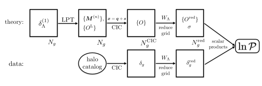
Figure 1: Flowchart of the steps involved in the computation of the forward model and likelihood. Three different grids are involved: $N_{g}$ is chosen to have a Nyquist frequency equal to or larger than $n\Lambda$, where $n$ is the order in perturbations of the forward model or bias expansion, whichever is larger; $N_{g}^{\rm CIC}=512$ is fixed; and $N_{g}^{\rm red}$ has a Nyquist frequency equal to $\Lambda$ (Eq. (2.9)). Both real and Fourier representations are involved on each grid.

4 Likelihood implementation details

We now describe the numerical details of the implementation of the real-space likelihood on a grid. Following the likelihood derived in [39], we generalize Eq. (2.3) to include a position-dependent variance $\sigma^{2}(\bm{x})$. As input, we take the data ${\delta}_{g}(\bm{x})$, which in our case is obtained from assigning a rest-frame halo catalog at a given redshift, and the set of Eulerian bias operators $O(\bm{x})$ constructed from the fixed initial conditions ${\delta}_{\rm in}$ (but varying $\sigma_{\mathrm{8}}$, which is implemented as described below). The steps for the computation of the likelihood thus start from the boxes labeled with $\{O\}$ and ${\delta}_{g}$ in the flowchart Fig. 1. The operator fields, combined with the bias parameters $b_{O}$, yield the deterministic field $\delta_{g,\rm det}[\{b_{O}\};\sigma_{\mathrm{8}};{\delta}_{\rm in}]$. The set of nuisance parameters consists of the $b_{O}$ as well as the parameters entering the variance $\sigma^{2}$; for this paper, this is only a single parameter $\sigma_{0}$, as discussed below.

As discussed in Sec. 2, we first reduce all grids, i.e. ${\delta}_{g}(\bm{x}),\,\delta_{g,\rm det}(\bm{x}),\,\sigma(\bm{x})$, from the base grid resolution $N_{g}$ to $N_{g}^{\rm red}$, where the Nyquist frequency of the reduced grid matches the cutoff $\Lambda$ (Eq. (2.9)). This reduction is done in Fourier space and requires some care to ensure the modes are properly mapped on the Nyquist planes (see Appendix B). While in Fourier space, we also set the $\bm{k}=\bm{0}$ mode in each operator as well as the data to zero, ensuring that all fields have vanishing mean. After the reduction, we then perform an inverse Fourier transform on the reduced grids, and evaluate the likelihood in real space:

$$-2\ln\mathcal{P}({\delta}_{g}|\{b_{O}\},\sigma_{0};\sigma_{\mathrm{8}};{\delta}_{\rm in})= \sum_{\bm{x}}^{N_{g}^{\rm red}}\frac{\left({\delta}_{g}(\bm{x})-\delta_{g,\rm det}[\{b_{O}\};\sigma_{\mathrm{8}};{\delta}_{\rm in}](\bm{x})\right)^{2}}{[\sigma(\bm{x})]^{2}}$$

$$+\frac{N_{\rm modes}}{(N_{g}^{\rm red})^{3}}\sum_{\bm{x}}^{N_{g}^{\rm red}}\ln\left(2\pi\frac{N_{g}^{6}}{(N_{g}^{\rm red})^{3}}[\sigma(\bm{x})]^{2}\right).$$ (4.1)

Notice that no explicit cutoff is necessary in the likelihood, since only modes with $|k_{i}|\leq\Lambda$ are represented on the grid. The normalization requires some explanation. First, we scale it from the number of real-space grid points $(N_{g}^{\rm red})^{3}$ to the actual number of independent modes $N_{\rm modes}$ computed as described in Appendix B. Further, we add a rescaling factor $N_{g}^{6}/(N_{g}^{\rm red})^{3}$, with which the log-likelihood for a constant $\sigma$ field returns the same value it would when evaluating the likelihood in Fourier space on a grid of size $N_{g}$. This is mostly done in order to cross-check the equivalence with the Fourier-space formulation; one can equivalently set $N_{g}=N_{g}^{\rm red}$ in this term without any impact on the inference, as it is an additive constant.

Eq. (4.1) is straightforward to evaluate, however still explicitly depends on the bias parameters, which requires one to search for a maximum in a high-dimensional parameter space. As shown in [34] and [39], it is possible to analytically marginalize over the bias parameters; this is because the log-likelihood Eq. (4.1) is a quadratic polynomial in the bias parameters (they enter linearly in $\delta_{g,\rm det}$). In the case that all bias parameters are marginalized over (in the notation of the above references, $\mu\to 0$), the likelihood becomes

$$-2\ln\mathcal{P}({\delta}_{g}|\sigma_{0};\sigma_{\mathrm{8}};{\delta}_{\rm in}) =C-\sum_{O,O^{\prime}}B_{O}(A^{-1})_{OO^{\prime}}B_{O^{\prime}}+\ln\det A$$

$$\quad+\frac{N_{\rm modes}}{(N_{g}^{\rm red})^{3}}\sum_{\bm{x}}^{N_{g}^{\rm red}}\ln\left(2\pi\frac{N_{g}^{6}}{(N_{g}^{\rm red})^{3}}[\sigma(\bm{x})]^{2}\right)+\ln\det{\rm C}_{\rm prior}\,,$$ (4.2)

where

$$C(\sigma_{0}) =\sum_{\bm{x}}^{N_{g}^{\rm red}}\,\frac{1}{[\sigma(\bm{x})]^{2}}\big{(}{\delta}_{g}(\bm{x})\big{)}^{2}$$ (4.3a)

$$B_{O}(\sigma_{0};\sigma_{\mathrm{8}};{\delta}_{\rm in}) =\sum_{\bm{x}}^{N_{g}^{\rm red}}\,\frac{{\delta}_{g}(\bm{x})O(\bm{x})}{[\sigma(\bm{x})]^{2}}+\sum_{O^{\prime}}({\rm C}_{\text{prior}}^{-1})_{OO^{\prime}}b^{\rm prior}_{O^{\prime}}$$ (4.3b)

$$A_{OO^{\prime}}(\sigma_{0};\sigma_{\mathrm{8}};{\delta}_{\rm in}) =\sum_{\bm{x}}^{N_{g}^{\rm red}}\,\frac{O(\bm{x})O^{\prime}(\bm{x})}{[\sigma(\bm{x})]^{2}}+({\rm C}_{\text{prior}}^{-1})_{OO^{\prime}}\,\,,$$ (4.3c)

while $b^{\rm prior}_{O}$ and $C_{\rm prior}$ denote the mean and covariance of a Gaussian prior on the bias parameters. While the code implementation allows for priors, for this paper we drop the prior terms, i.e. formally send $C_{\rm prior}^{-1}\to 0$, corresponding to a uniform prior on the bias parameters. Note that the $O(\bm{x})$, and hence $B_{O}$ and $A_{OO^{\prime}}$, depend on $\sigma_{\mathrm{8}}$ and ${\delta}_{\rm in}$ via the forward model. In this paper, we always show results marginalized over all $b_{O}$ (while Refs. [34, 38] did not marginalize over $b_{1}$).

All the grid operations are straightforwardly parallelized (using OpenMP in our implementation). For the matrix operations (inverse and determinant), we use the LU decomposition with full column pivoting as provided by the Eigen C++ library [47]. Specifically, we write

$$\sum_{O,O^{\prime}}B_{O}(A^{-1})_{OO^{\prime}}B_{O^{\prime}}=\bm{B}^{\top}\cdot\bm{X}\quad\mbox{where $\bm{X}$ satisfies}\quad\bm{A}\cdot\bm{X}=\bm{B},$$ (4.4)

avoiding the explicit computation of the matrix inverse.

The computation of the $\sigma_{\mathrm{8}}$ profile likelihood proceeds by finding the maximum of the likelihood Eq. (4.2) over all free parameters for a range of $\sigma_{\mathrm{8}}$ values [34]. Specifically, we determine the maximum log-likelihood for the values

$$A_{\rm in}\equiv\frac{\sigma_{\mathrm{8}}}{\sigma_{\mathrm{8}}^{\rm fid}}\in\{0.9,\ 0.95,\ 0.98,\ 1.00,\ 1.02,\ 1.05,\ 1.1\},$$ (4.5)

which yields the profile likelihood $P_{\rm prof}(A_{\rm in})$. The different values of $A_{\rm in}$ are implemented by rescaling the fiducial linear density field used to generate the initial conditions of the N-body simulations by the factor $A_{\rm in}$ before constructing the LPT forward model and bias operators; i.e., we use ${\delta}_{\rm in}(\bm{x})=A_{\rm in}{\delta}_{\rm in}^{\rm fid}(\bm{x})$ (hence the subscript on $A_{\rm in}$). In order to obtain a precise representation of ${\delta}_{\rm in}^{\rm fid}(\bm{x})$, we have modified the initial conditions generator of Ref. [48] (which is based on that of [49]) to write the linear density field to disk, before it is used to generate the 2LPT particle displacements. Again, unlike the results in previous papers in this series, the final matter density field comes out of the nLPT forward model and is not taken from an external code or simulations. As described in [34, 38], the maximum-likelihood value $\hat{A}_{\rm in}$ and its error are determined through the maximum and curvature around the maximum of $P_{\rm prof}(A_{\rm in})$.

In our case, where the initial phases and hence the bias operators constructed from them are fixed, the only free parameters remaining in Eq. (4.2) at fixed value of $\sigma_{\mathrm{8}}$ (equivalently $A_{\rm in}$) are those entering the variance: the constant variance parameter $\sigma_{0}$, corresponding to the square-root of the spatial average of $P_{\varepsilon}(\bm{x})$, and one free coefficient for each relevant stochastic operator. This maximization is done using Minuit as implemented in the root package. Unfortunately, the profile likelihood is easily spoiled if significantly different maximum-likelihood values of $\sigma_{0}$ are found at different values of $A_{\rm in}$, for example due to numerical instabilities in the maximization; variations in $\sigma_{0}$ at the few-percent level are already sufficient to lead to significant noise in $\hat{A}_{\rm in}$. While this issue is manageable for the $o=3$ expansion, it becomes progressively worse at higher orders. For this reason, we do not consider a field-dependent covariance here, but instead restrict the covariance to a constant, $\sigma^{2}(\bm{x})=\sigma_{0}^{2}$. Notice that this issue should be alleviated once a full joint sampling of $\sigma_{\mathrm{8}}$ and the stochastic parameters is performed, since then the likelihood is evaluated consistently at each point in the joint parameter space. Apart from this numerical issue, we have found that the field-dependent covariance only has a minor impact on the $\sigma_{\mathrm{8}}$ inference. We discuss this in Sec. 6.1.

Finally, in order to determine the maximum-likelihood value $\hat{A}_{\rm in}$ and its error from the profile likelihood, we fit a quadratic polynomial to the log-likelihood, which yields $\hat{A}_{\rm in}$ as the point of maximum and the estimated error as the inverse square root of the curvature.

5 Results

We now present results for the maximum-likelihood value of $\sigma_{\mathrm{8}}$ (or equivalently $\mathcal{A}_{s}$) inferred from rest-frame halo catalogs for fixed initial phases, phrased in terms of the maximum-profile-likelihood value $\hat{A}_{\rm in}$. Unbiased inference corresponds to values of $\hat{A}_{\rm in}$ that are consistent with 1 within errors. The default halo catalogs are the same as those used in [34, 38], and are described in Appendix C; they consist of four sharp, disjoint mass bins covering the range $10^{12.5}-10^{14.5}\,h^{-1}M_{\odot}$ at redshifts $0,0.5,1$, identified in two simulation realizations of $(2000\,h^{-1}\text{Mpc})^{3}$ volume each. The only difference to the samples reported on in previous work is that we now use halos identified in N-body simulations with a starting redshift $z_{\rm in}=24$ instead of 99, as employed in the previous papers in this series. The reason is discussed in Sec. 6.

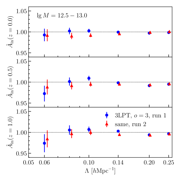
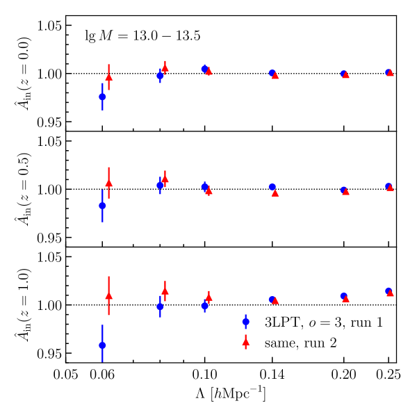
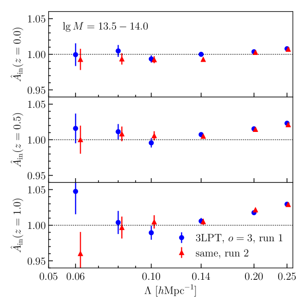
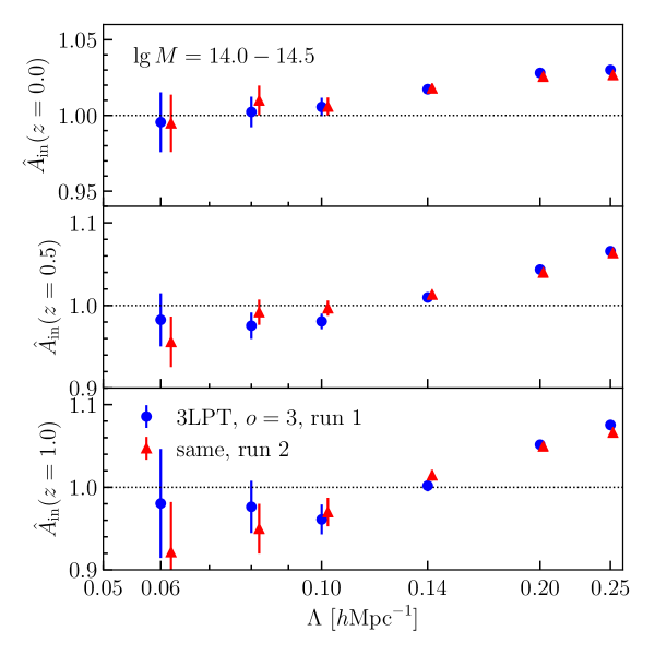
Figure 2: Results on the estimated value of $\sigma_{\mathrm{8}}$, relative to the ground truth, as a function of cutoff value $\Lambda$. The different panels show the four mass bins considered (with $M$ in units of $\,h^{-1}M_{\odot}$), and each panel shows the results for three redshifts: $z=0,\,0.5,\,1$. The results shown are for 3LPT with an $o=3$ bias expansion, and for two simulation realizations. The scatter between the two simulation realizations is consistent with the statistical errors inferred from the profile likelihood.

Fig. 2 shows the results for the 3LPT forward model with a third-order bias expansion; more precisely, $o=3$ in the ordering described in Sec. 3.2. The reported error bars, which take into account both halo stochasticity and cosmic variance (see below), clearly grow for the more rare high-mass halo samples at higher redshifts.

The expected convergence to $\hat{A}_{\rm in}=1$ as $\Lambda\to 0$ is seen for all masses and redshifts. Note that the inferred $\sigma_{\mathrm{8}}$ value never differs from the truth by more than $\sim 4\%$ for all our samples and all cutoff values considered. Excluding the lowest cutoff value, which has the largest statistical error bars, as well as the highest cutoff value $\Lambda=0.25\,h\,\text{Mpc}^{-1}$, which is close to the nonlinear scale at $z=0$, the $\sigma_{\mathrm{8}}$ inference is in fact accurate to 2% or better for all samples for this third-order forward model. The rate at which $\hat{A}_{\rm in}$ diverges from 1 when going to larger $\Lambda$ clearly depends on halo mass and redshift. We return to this point below when comparing results at different orders $o$.

Fig. 2 shows results for both simulation realizations. Note that, since the phases are fixed to the true values used in the initial conditions for each simulation realization, the only source of cosmic variance between the two realizations is due to the different realizations of the modes above the cutoff $\Lambda$. Thus, at fixed cutoff value and halo sample, the results from different simulation realizations are sampled from the same underlying distribution. The width of this distribution should, if the EFT likelihood is accurate, be correctly captured by the statistical error inferred from the profile likelihood, which is controlled by the effective noise amplitude $\sigma_{0}$. Note that the previous papers in this series [33, 34, 38] incorrectly suggested that there would be an additional cosmic variance contribution to the error on $\hat{A}_{\rm in}$ beyond that given by the profile likelihood.

Indeed, the scatter between the results from the two realizations in Fig. 2 is consistent with the statistical error bar inferred from the profile likelihood. We have verified this by histogramming the quantity $(\hat{A}_{\rm in}({\rm run\ 1})-\hat{A}_{\rm in}({\rm run\ 2}))/\sqrt{\sigma^{2}({\rm run\ 1})+\sigma^{2}({\rm run\ 2})}$ for the results shown in Fig. 2, i.e. combining all cutoff values and halo samples. The resulting distribution has an RMS of $1.2\pm 0.1$, indicating that, in addition to unbiased inference of $\hat{A}_{\rm in}$ on large scales, the EFT likelihood also correctly estimates the error on $\hat{A}_{\rm in}$.

Comparison to Fourier-space likelihood: before continuing, it is worth comparing the results of the real-space likelihood to that of the Fourier-space likelihood employed in [34, 38], using the same Lagrangian forward model and bias expansion for both likelihoods in order to restrict the comparison to the likelihood itself. This is shown in Fig. 8 in Appendix A. Note that the real-space likelihood employs a cubic $k$ cut, while the Fourier-space implementation of [34, 38] employs a spherical cut. Hence, the modes used in each case are not the same, and we do not expect exact agreement. In fact, the real-space likelihood employs modes with slightly larger wavenumber, up to $\sqrt{3}\Lambda$ as compared to $\Lambda$ for the spherical cut; the effect of this is visible for the lowest values of $\Lambda$, where the error bars in the Fourier-space likelihood results are noticeably larger than the corresponding real-space ones. Given these differences, we find very good agreement.

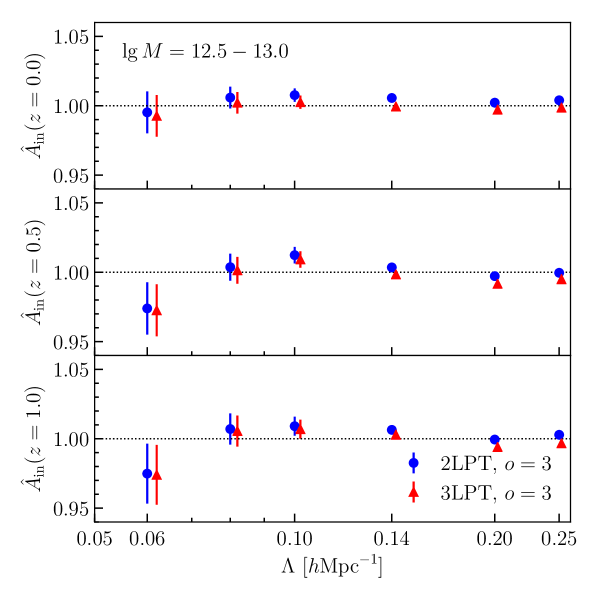
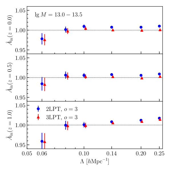
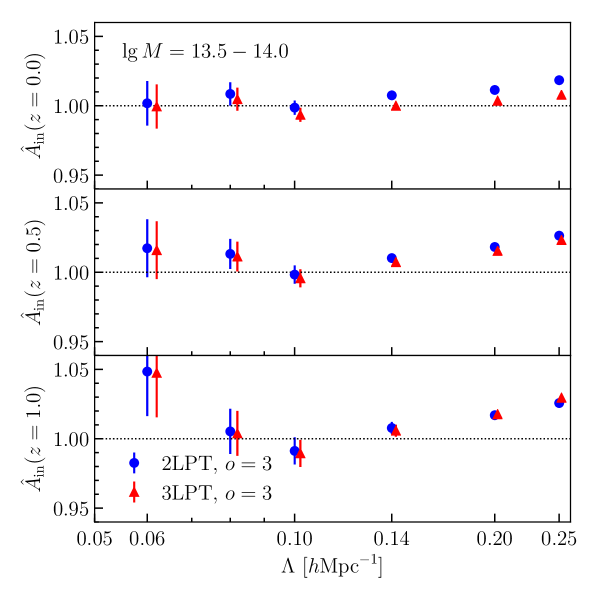
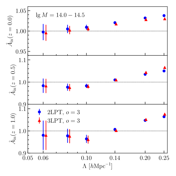
Figure 3: Same as Fig. 2, comparing results using 2LPT and 3LPT forward models, both with an $o=3$ bias expansion. Results for run 1 are shown here and in all following figures.

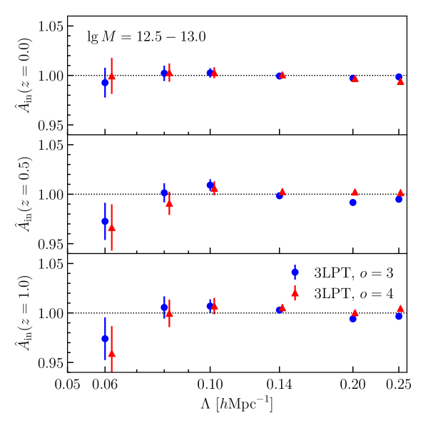
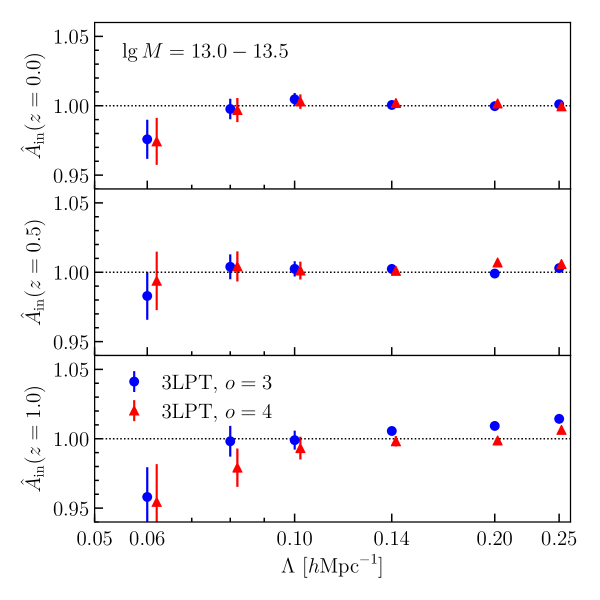
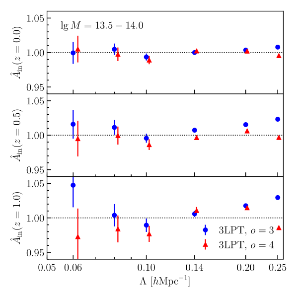
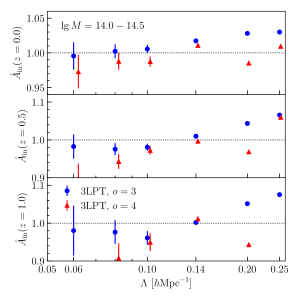
Figure 4: Same as Fig. 2, comparing results using 3LPT forward model, with an $o=3$ vs $o=4$ bias expansion.

Effect of LPT order: Fig. 3 compares results of second- and third-order LPT (2LPT and 3LPT, respectively), both for the $o=3$ bias expansion. The results are similar, but since 3LPT yields more power in the density field and displacement, the estimated value of $\hat{A}_{\rm in}$ generally moves down slightly when compared to 2LPT. In most cases, this moves $\hat{A}_{\rm in}$ closer to unity.

Effect of bias order: Fig. 4 compares results for 3LPT with the $o=3$ (as in Fig. 2) and the $o=4$ bias expansions. For cutoffs $\Lambda\leq 0.1\,h\,\text{Mpc}^{-1}$, the fourth-order bias terms do not change the $\sigma_{\mathrm{8}}$ inference, except for the rarest halo samples where they actually appear to lead to increased scatter; note that the $o=4$ bias expansion marginalizes over 19 parameters, compared to 8 for $o=3$ (Tab. 1). For higher cutoff values, the $o=4$ case does perform somewhat better, essentially increasing the reach of the forward model of the halo density field to smaller scales. Similar conclusions hold when going to even higher order, $o=5$, which increases the number of free parameters by another factor of 2. This trend becomes even clearer when plotting $\hat{A}_{\rm in}$ at fixed $\Lambda$ for the different halo samples.

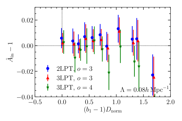
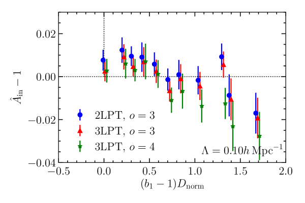
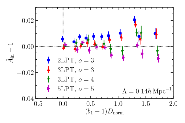
Figure 5: Maximum-likelihood value $\hat{A}_{\rm in}-1$ for all halo samples and redshifts (but for one simulation realization only) at a fixed cutoff value. The x axis shows the combination $(b_{1}-1)D_{\rm norm}$, where $D_{\rm norm}=D(z)/D(0)$ is the normalized growth factor at the redshift of the given sample. The different panels show different cutoff values as indicated. In each panel, we show results for different forward model/bias expansions. This gives an overview of the overall performance of different expansions at different cutoff values.

$\bm{A_{\rm in}}$ vs. bias: So far, we have discussed $\hat{A}_{\rm in}$ as a function of cutoff $\Lambda$ for individual halo samples. Fig. 5 shows an alternative representation, where all halo mass bins and redshifts are plotted in a single panel, but at fixed cutoff. This gives a good overview of the performance of a given expansion order at a fixed cutoff. We choose to plot results as the fractional deviation of the inferred $\sigma_{\mathrm{8}}$ value from the truth, i.e. $\hat{A}_{\rm in}-1$, as a function of the combination $b_{1}D_{\rm norm}$ where $b_{1}$ is the linear bias and $D_{\rm norm}=D(z)/D(0)$ is the normalized growth factor at the redshift of the given halo sample. As argued in [38], $b_{1}D_{\rm norm}$ is a rough indicator for the magnitude of higher-order bias contributions (that is, higher order in perturbations rather than derivatives). Since we marginalize over $b_{1}$ here, we adopt the values for $b_{1}$ reported in [38] for the same halo samples using the third-order likelihood; this is entirely sufficient for this purpose. The different panels in the figure show different cutoff values. Some interesting trends can be gleaned from this representation:

• For $\Lambda=0.08\,h\,\text{Mpc}^{-1}$, all results are consistent with $\hat{A}_{\rm in}=1$ within errors; no significant improvement is seen for higher LPT or bias orders.

• At $\Lambda=0.1\,h\,\text{Mpc}^{-1}$, deviations start to become statistically mildly significant for the most highly biased samples, in agreement with the conclusions of [38].

• For $\Lambda=0.14\,h\,\text{Mpc}^{-1}$, the deviations are now significant statistically, albeit not much larger in magnitude; for this cutoff value, going from 2LPT to 3LPT, and from $o=3$ to $o=4$ bias expansions each reduce the bias in $\sigma_{\mathrm{8}}$ significantly. The results for $o=5$ do not generally improve upon those with $o=4$ for the more highly biased samples, likely because the fifth-order contributions are still small on those scales.

• $\Lambda=0.2\,h\,\text{Mpc}^{-1}$: Similar conclusions hold as for $\Lambda=0.14\,h\,\text{Mpc}^{-1}$, except that the $o=5$ bias expansion now marginally improves the residuals over $o=4$ as well.

To summarize, we find the expected reduction in the systematic bias on the inferred $\sigma_{\mathrm{8}}$ value when lowering $\Lambda$ at fixed bias order, or when increasing the bias order at fixed $\Lambda$. The exception is that for $o>3$, some instabilities appear at lower values of $\Lambda$, especially for the rare halo samples. It would be interesting to revisit this issue with full sampling instead of the profile likelihood. In any case, we find that in all cases where these instabilities appear, a lower-order bias expansion is sufficient to yield unbiased results to within errors (e.g., $o=3$ for $\Lambda=0.1\,h\,\text{Mpc}^{-1}$, or $o=4$ for $\Lambda=0.14\,h\,\text{Mpc}^{-1}$). Overall, it appears that not much improvement is obtained when going beyond $o=4$.

It is also worth noting that the inferred statistical errors on $\hat{A}_{\rm in}$ at fixed $\Lambda$ do not grow significantly when going to higher orders in the expansion, despite the additional free parameters that are being marginalized over.

6 Discussion

We now discuss investigations on issues apart from the expansion order and halo mass and redshift presented above.

6.1 Position-dependent variance

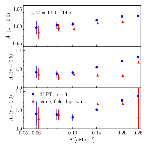
Figure 6: Effect of allowing for a position-dependent variance, in case of the $o=3$ bias expansion.

The results shown so far are based on a constant variance field $\sigma^{2}(\bm{x})=\sigma_{0}^{2}$. At the order in perturbations that we work in however, field-dependent terms in the variance formally become significant. The effect of the density-dependent variance on the inference is essentially to upweight regions of less noise, and downweight regions with higher noise. Thus, even if the density-dependent variance is formally relevant in perturbation theory, we expect the constant-variance case to be merely suboptimal, but not necessarily biased.

Fig. 6 compares results allowing for a position-dependent variance including the relevant terms at order $o=3$. Specifically, the variance field is written as the square of

$$\sigma(\bm{x})=\sigma_{0}\left[1+\sum_{O}r^{\varepsilon}_{O}O(\bm{x})\right],$$ (6.1)

where the sum runs over all operators that are relevant for the case considered (using Eq. (3.17) with $k=1$).

We find that for moderately biased samples, the results are compatible in most cases, although the constant-variance results are generally less biased. More significant differences are visible for the more highly biased samples. However, the results with position-dependent variance are overall less stable than the constant-variance case. We attribute this to the numerical issues discussed in Sec. 4; indeed, the profile likelihoods show several outliers for these highly biased cases, for which the value of $\sigma_{0}$ differs significantly between neighboring values of $A_{\rm in}$, which is not expected physically. It is clearly worth revisiting this issue using a full sampling approach.

6.2 Beyond the Einstein-de Sitter approximation

We now turn to the impact of the EdS approximation. As discussed in Sec. 3, we do not consider additional bias terms induced beyond EdS, which appear at fourth order in perturbations. However, the LPT implementation incorporates general expansion histories [40], so we can determine the effect of going beyond the EdS approximation in LPT itself, which formally appears already at second order in perturbations, where $D_{2}\neq D^{2}$. Note that we always use the linear growth factor $D$ for the $\Lambda$CDM simulation cosmology. This comparison is shown in Fig. 9 in Appendix A. Both cases agree to within fractions of a percent. We conlude that the EdS approximation is not a significant source of systematic uncertainty at this level.

6.3 N-body accuracy

In any study involving simulation results, a quantification of the numerical error in the simulations is in order. Here, we are only concerned with numerical issues that could affect the $\sigma_{\mathrm{8}}$ inference; this also includes the halo finder used to construct the halo sample (we turn to this in the next section). Given the general bias expansion that the forward model is built on, any issue that can be captured by small-scale noise and error in the force calculation should not lead to a bias in $\sigma_{\mathrm{8}}$, as all local effects are captured by bias terms and the noise covariance.

Following this reasoning, the N-body aspects of most concern are the accuracy of the time integration, as this could potentially affect the accurate calculation of the growth of the large-scale perturbations, and transients from the initial conditions. We have investigated the former effect by performing a re-simulation of our fiducial realization with increased accuracy: specifically, we changed the Gadget2 parameters as follows:

ErrTolIntAccuracy: $$\quad 0.025\to 0.01$$

MaxRMSDisplacementFac: $$\quad 0.2\to 0.1$$

MaxSizeTimestep: $$\quad 0.025\to 0.01\,.$$

We have not found even a slight effect on the $\sigma_{\mathrm{8}}$ inference, concluding that the standard Gadget2 precision settings employed in our fiducial simulations are entirely sufficient at the percent level.

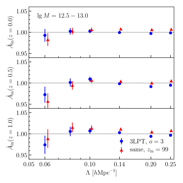
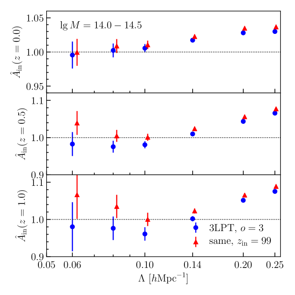
Figure 7: Effect of varying the initial redshift of the N-body simulations in which the halo samples are identified; 2LPT is used to initialize the simulations in both cases. The blue points show the fiducial case of $z_{\rm in}=24$ adopted in this paper, while red points show $z_{\rm in}=99$, corresponding to the simulations used in previous references.

The conclusions are quite different for transients from the initial conditions, which in our case are always obtained from 2LPT, leaving the choice of starting redshift $z_{\rm in}$ for the N-body simulations. This is a subtle issue, as starting later (lower $z_{\rm in}$) leads to inaccuracies due to incorrect nonlinear evolution, while starting earlier (higher $z_{\rm in}$) leads to artefacts because of the grid on which the particles are initially placed (“pre-initial conditions”) and the associated noise. While the simulations initially performed for [50] were started at $z_{\rm in}=99$, we here choose a significantly later starting redshift of $z_{\rm in}=24$ following the reasoning of [46, 51]. Ideally, one would use a higher-order LPT implementation to generate the initial conditions, but we refer this to future work.

This choice is verified by the $\sigma_{\mathrm{8}}$ inference, as shown in Fig. 7: there are percent-level shifts between $z_{\rm in}=24$ and $z_{\rm in}=99$ in some cases, with the former results being closer to unbiased. A systematic investigation of the best choice of starting redshift is deferred to future work. Clearly however, systematic errors due to transients cannot be neglected when evaluating the accuracy of the $\sigma_{\mathrm{8}}$ inference from perturbative approaches.

6.4 Halo sample

Following the discussion in the previous section, we do not expect the $\sigma_{\mathrm{8}}$ inference to depend in any significant way on the halo finder and mass definition employed, as long as the mass is determined from locally observable quantities, such as the density (or distance to the nearest neighbor particle) and relative velocity of a particle with respect to the halo center. Thus, the requirements for a $\sigma_{\mathrm{8}}$ inference accurate to 1% are much less stringent than, say, for a 1% measurement of the halo mass function.

As an illustration, Fig. 10 (Appendix A) shows the comparison of the $\sigma_{\mathrm{8}}$ results obtained from a halo sample obtained from the Rockstar halo finder (see Appendix C for details) and our fiducial set. No significant differences are found. We have also performed an analysis excluding subhalos from our fiducial sample. We again find no significant difference to the fiducial case (only a modest fraction of our fairly high-mass halos are subhalos).

7 Conclusions

We have presented a real-space implementation of the EFT likelihood, which allows for the straightforward incorporation of observational effects such as the survey window function. The EFT likelihood marginalizes precisely over those parts of the likelihood $\mathcal{P}({\delta}_{g}|\{b_{O},\sigma_{0}\},\sigma_{\mathrm{8}})$ of a biased tracer density field ${\delta}_{g}$ that are affected by nonlinear, spatially local but temporally nonlocal structure formation. The real-space formulation was previously presented in [39], but its actual implementation involves some subtleties in the grid reduction (Appendix B). We presented results on the inference of $\sigma_{\mathrm{8}}$ from a rest-frame halo catalog using the real-space likelihood and a new Lagrangian forward model described in detail in an upcoming paper [40]. As in previous papers in this series, we marginalize analytically over the substantial number of free bias parameters (up to 42).

Our numerical results, presented in Sec. 5 and perhaps best summarized by Fig. 5, fully show the expected convergence behavior as a function of scale, for the different expansion orders considered. Compared to the recent Ref. [38], which employed a Eulerian bias expansion with an additional cutoff, the accuracy of the $\sigma_{\mathrm{8}}$ inference has further improved. For cutoff values $\Lambda\leq 0.14\,h\,\text{Mpc}^{-1}$, the residual bias in $\sigma_{\mathrm{8}}$ is less than 2%, and within 1% for the majority of halo samples.

Bias models beyond cubic order, $o=4$ and $o=5$, further improve the $\sigma_{\mathrm{8}}$ inference over the cubic expansion for higher cutoff values $\Lambda>0.14\,h\,\text{Mpc}^{-1}$, in particular for the more highly biased samples. Somewhat surprisingly, the bias in $\sigma_{\mathrm{8}}$ remains under control even for a cutoff value of $\Lambda=0.25\,h\,\text{Mpc}^{-1}$, which approaches the nonlinear scale. This is likely partially explained by the fact that the small scales are already shot noise dominated for most of the halo samples; we still generally find a reduction in the statistical error bar on $\sigma_{\mathrm{8}}$ by a factor of $0.5-0.7$ between $\Lambda=0.2\,h\,\text{Mpc}^{-1}$ and $\Lambda=0.25\,h\,\text{Mpc}^{-1}$ however (the statistical error is on the order of 0.1% or less for the latter cutoff, and not visible in the plots).

Having improved substantially on the previous results of [38], this is likely to be the most precise inference (in terms of statistical as well as systematic error) of cosmological parameters from purely nonlinear information in biased tracers of large-scale structure—albeit fixing the phases and other cosmological parameters.

The connection to observations will require the incorporation of redshift-space distortions and the window function. We have argued here that the latter is straightforward within the real-space formulation. We plan to investigate this next. Regarding the former, this is likewise straightforward within the EFT likelihood framework, by transforming the deterministic field $\delta_{g,\rm det}$ to redshift space, and incorporating the Jacobian [52]. The Lagrangian forward model employed here is in fact ideally suited for this task. We leave an implementation of this to future work as well.

Appendix A Supplementary figures

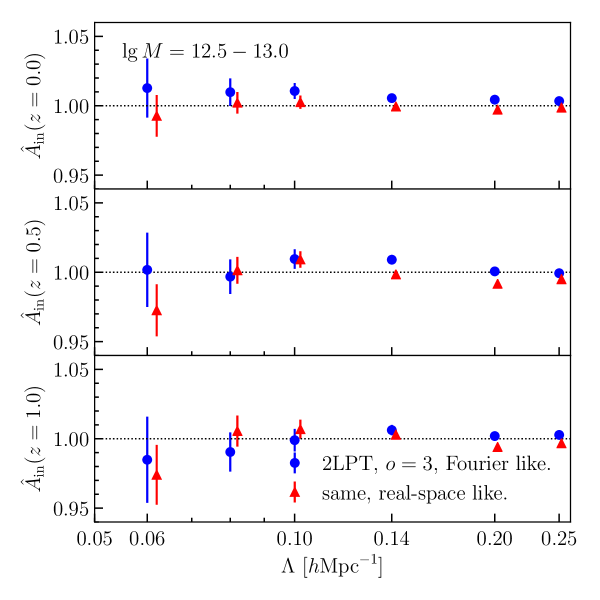
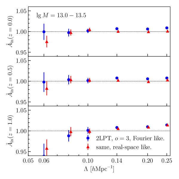
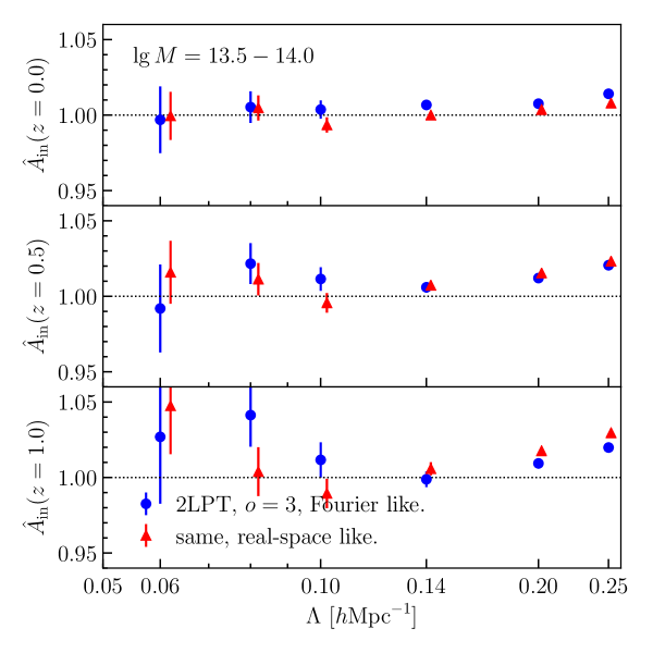
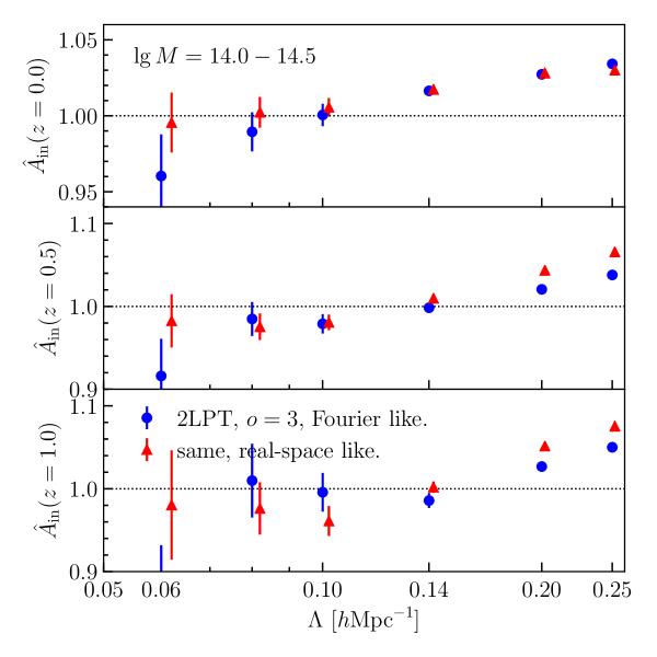
Figure 8: Same as Fig. 2, but comparing results from real-space and Fourier-space likelihoods. Here, a 2LPT forward model using a $o=3$ bias expansion is used, corresponding to the third-order case of [38] (but using a Lagrangian rather than Eulerian bias expansion). Results here and in all following figures are for run 1.

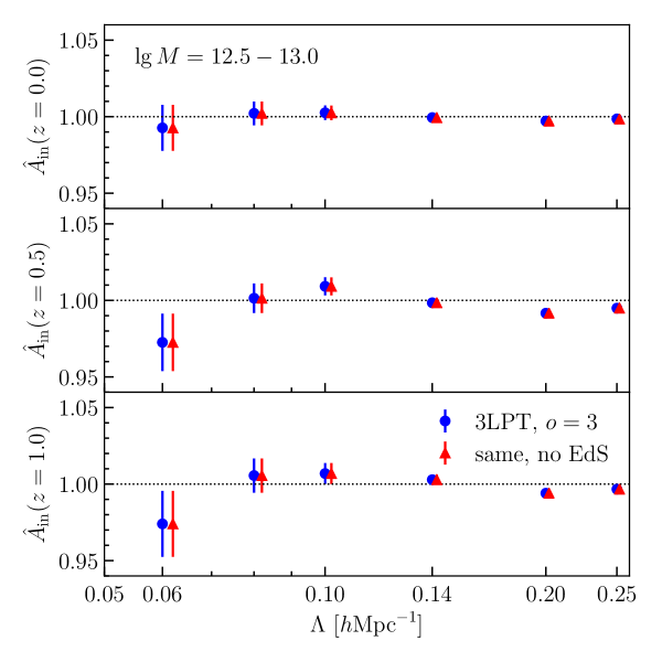
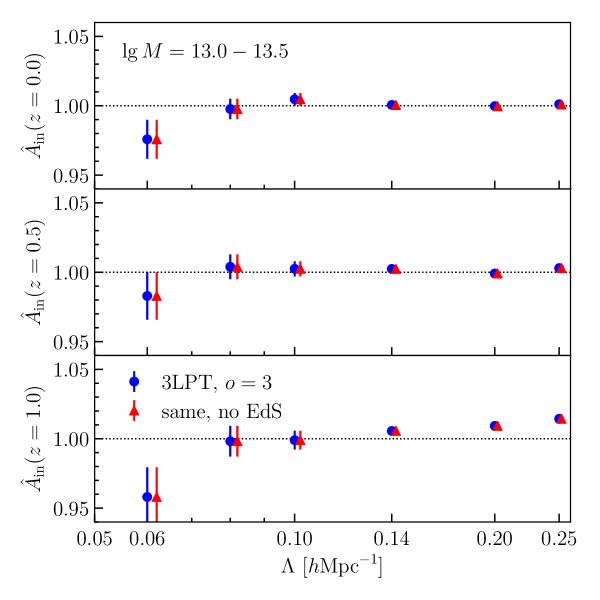
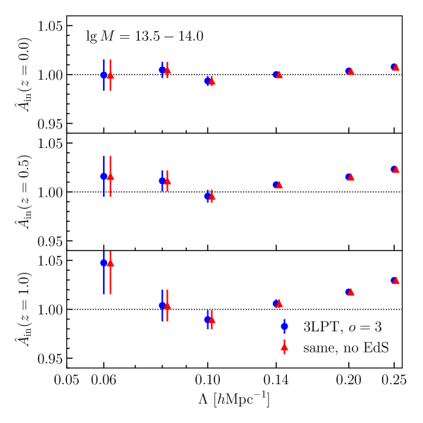
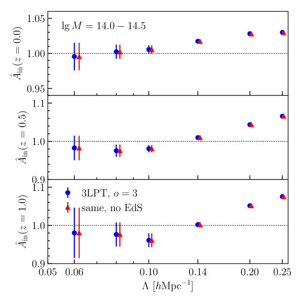
Figure 9: Effect of relaxing the assumption of the EdS approximation in the LPT forward model. The results are essentially unchanged.

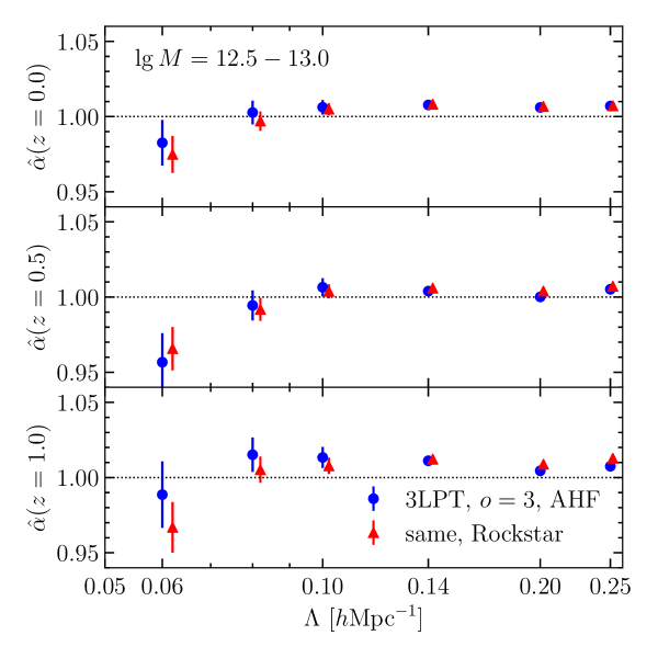
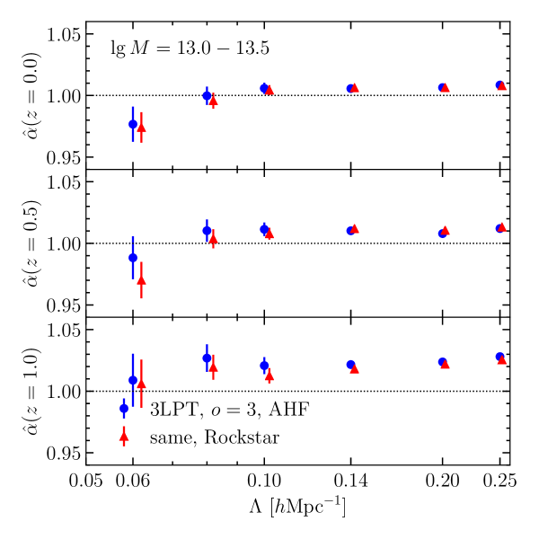
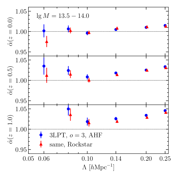
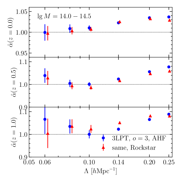
Figure 10: Results for the same likelihood as in Fig. 2, comparing the results of the fiducial AHF halo catalog with Rockstar halos. Note that both halo samples shown here were identified in simulations with $z_{\rm in}=99$.

Appendix B Grid reduction in Fourier space

An essential step in the real-space likelihood computation is the reduction from a Fourier-space grid with $k_{\rm Ny}\gg\Lambda$ to one where $k_{\rm Ny}=\Lambda$. We now describe how this is implemented. First, we determine the size of the reduced grid via

$$N_{g}^{\rm red}=2\left\lfloor\frac{\Lambda L_{\rm box}}{2\pi}\right\rfloor\,,$$ (B.1)

where the floor function reduces $N_{g}^{\rm red}$ to the next even number, which is desirable for numerical reasons. Thus, the actual cutoff is slightly smaller than $\Lambda$; in practice this difference is at most $0.006\,h\,\text{Mpc}^{-1}$ for the box size considered here.

For all Fourier modes $\bm{k}$ with $k_{i}<k_{\rm Ny}^{\rm red}/2$, where $k_{i}$ denote the Cartesian components of $\bm{k}$, we then simply copy over the Fourier modes from the larger grid, scaling them by the discrete FFT normalization factor $(N_{g}^{\rm red}/N_{g})^{3}$. For these modes the Hermitianity of the resulting field (${\delta}(-\bm{k})={\delta}^{*}(\bm{k})$ for a field ${\delta}$) is ensured by way of the Hermitianity of the input field on the full grid. The modes on the Nyquist planes, for which $k_{i}=\pm k_{\rm Ny}^{\rm red}/2$ for at least one $i=1,2,3$, need to be handled slightly differently, because several (nonzero) modes of the full grid are mapped onto the same mode on the reduced grid.

First, we set the imaginary part of these modes to zero, as required for Hermitianity. Second, we multiply the real part of each mode on the Nyquist planes by a factor $\sqrt{w}$, where $w$ counts the number of modes on the full grid that are mapped onto the given mode on the reduced grid. Specifically,

• $w=2$ for modes on the faces of the Nyquist cube (a single component $k_{i}=\pm k_{\rm Ny}^{\rm red}/2$), since three of the six faces are represented on the reduced grid;

• $w=4$ for modes on the edges (two components $k_{i},k_{j}=\pm k_{\rm Ny}^{\rm red}/2$ with $i\neq j$), since 3 out of 12 edges are represented on the reduced grid;

• $w=8$ for the single reduced-grid mode on the corner (all three components equal to $\pm k_{\rm Ny}^{\rm red}/2$; at the center of the reduced grid in terms of memory layout), since all 8 corners are mapped onto this mode.

This procedure ensures that, in the ensemble average, the modes on the reduced grid have the same power as that on the full grid, which they should since all modes that are nonzero on the full grid should be represented on the reduced grid. We have verified that for a field ${\delta}(\bm{k})$, the norm $\sum_{\bm{k}}|{\delta}(\bm{k})|^{2}$ agrees to a fractional precision of order $1/N_{g}^{\rm red}$ between the full and reduced grids, the residual deviation being random fluctuations due to the modes on the Nyquist planes.

Finally, we ensure the Hermitianity of the resulting field by setting ${\delta}(-\bm{k})={\delta}^{*}(\bm{k})$. We do this by running only over the half-volume with $k_{x}\geq 0$, where the modes with $k_{x}<0$ are determined by the Hermitianity condition. This procedure also allows for efficient parallelization by dividing up the $k_{x}$ loop over threads (where the otherwise problematic $k_{x}=0$ plane is assigned to a single thread).

Finally, the effective number of modes on the reduced grid is

$$N_{\rm modes}=(N_{g}^{\rm red})^{3}+3(N_{g}^{\rm red})^{2}+3N_{g}^{\rm red}+1.$$ (B.2)

Appendix C Halo catalogs

All numerical tests presented here are based on a set of N-body simulations analagous to those used in [34, 38], which were presented in [50]. They are generated using GADGET-2 [49] for a flat $\Lambda$CDM cosmology with parameters $\Omega_{\mathrm{m}}=0.3$, $n_{\mathrm{s}}=0.967$, $h=0.7$, and $\sigma_{\mathrm{8}}=0.85$, a box size of $L=2000\,h^{-1}\mathrm{Mpc}$, and $1536^{3}$ dark matter particles of mass $M_{\mathrm{part}}=1.8\times 10^{11}\,h^{-1}M_{\odot}$. Two realizations are available, which we refer to as “run 1” and “run 2.” We do not use the simulations generated for [50], but instead have rerun them for the same initial phases but a later starting redshift of $z_{\rm in}=24$ instead of 99 (see Sec. 6.3).

Dark matter halos were subsequently identified at different redshifts as spherical overdensities [53, 54, 55] applying the Amiga Halo Finder algorithm (AHF) [56, 57] with an overdensity threshold of $200$ times the background matter density.

For comparison, we have also generated halo catalogs using Rockstar [58] (Sec. 6.4). We used the same $\Delta=200b$ mass definition and the option STRICT_SO_MASSES.

References

- [1] T. Baldauf, M. Mirbabayi, M. Simonović and M. Zaldarriaga, LSS constraints with controlled theoretical uncertainties, 1602.00674.
- [2] T. Nishimichi, G. D’Amico, M. M. Ivanov, L. Senatore, M. Simonović, M. Takada et al., Blinded challenge for precision cosmology with large-scale structure: results from effective field theory for the redshift-space galaxy power spectrum, 2003.08277.
- [3] A. Chudaykin, M. M. Ivanov and M. Simonović, Optimizing large-scale structure data analysis with the theoretical error likelihood, 2009.10724.
- [4] D. J. Eisenstein, H.-J. Seo, E. Sirko and D. N. Spergel, Improving Cosmological Distance Measurements by Reconstruction of the Baryon Acoustic Peak, ApJ 664 (Aug., 2007) 675–679, [astro-ph/0604362].
- [5] N. Padmanabhan, M. White and J. D. Cohn, Reconstructing baryon oscillations: A Lagrangian theory perspective, PhRvD 79 (Mar., 2009) 063523, [0812.2905].
- [6] V. Desjacques, D. Jeong and F. Schmidt, Large-scale galaxy bias, PhR 733 (Feb., 2018) 1–193, [1611.09787].
- [7] Z. Zheng, R. Cen, H. Trac and J. Miralda-Escude, Radiative transfer modeling of Ly emitters. II. New effects in galaxy clustering, Astrophys. J. 726 (2010) 38–64, [1003.4990].
- [8] S. Wyithe and M. Dijkstra, Non-gravitational contributions to the clustering of Ly selected galaxies: Implications for cosmological surveys, Mon. Not. Roy. Astron. Soc. 415 (2011) 3929, [1104.0712].
- [9] C. Behrens, C. Byrohl, S. Saito and J. Niemeyer, The impact of Lyman- radiative transfer on large-scale clustering in the Illustris simulation, Astron. Astrophys. 614 (2018) A31, [1710.06171].
- [10] E. Krause and C. Hirata, Tidal alignments as a contaminant of the galaxy bispectrum, Mon. Not. Roy. Astron. Soc. 410 (2011) 2730, [1004.3611].
- [11] D. Martens, C. M. Hirata, A. J. Ross and X. Fang, A radial measurement of the galaxy tidal alignment magnitude with BOSS data, Mon. Not. Roy. Astron. Soc. 478 (2018) 711–732, [1802.07708].
- [12] A. Obuljen, N. Dalal and W. J. Percival, Anisotropic halo assembly bias and redshift-space distortions, JCAP 1910 (2019) 020, [1906.11823].
- [13] V. Desjacques, D. Jeong and F. Schmidt, The galaxy power spectrum and bispectrum in redshift space, JCAP 1812 (2018) 035, [1806.04015].
- [14] N. Agarwal, V. Desjacques, D. Jeong and F. Schmidt, Information content in the redshift-space galaxy power spectrum and bispectrum, 2007.04340.
- [15] E. Bertschinger and A. Dekel, Recovering the full velocity and density fields from large-scale redshift-distance samples, ApJL 336 (Jan., 1989) L5–L8.
- [16] O. Lahav, K. B. Fisher, Y. Hoffman, C. A. Scharf and S. Zaroubi, Wiener Reconstruction of All-Sky Galaxy Surveys in Spherical Harmonics, ApJL 423 (Mar., 1994) L93, [astro-ph/9311059].
- [17] K. B. Fisher, O. Lahav, Y. Hoffman, D. Lynden-Bell and S. Zaroubi, Wiener reconstruction of density, velocity and potential fields from all-sky galaxy redshift surveys, MNRAS 272 (Feb., 1995) 885–908, [astro-ph/9406009].
- [18] I. M. Schmoldt, V. Saar, P. Saha, E. Branchini, G. P. Efstathiou, C. S. Frenk et al., On Density and Velocity Fields and beta from the IRAS PSCZ Survey, AJ 118 (Sept., 1999) 1146–1160, [astro-ph/9906035].
- [19] P. Erdodu, O. Lahav, S. Zaroubi, G. Efstathiou, S. Moody, J. A. Peacock et al., The 2dF Galaxy Redshift Survey: Wiener reconstruction of the cosmic web, MNRAS 352 (Aug., 2004) 939–960, [astro-ph/0312546].
- [20] J. Jasche, F. S. Kitaura, B. D. Wandelt and T. A. Enßlin, Bayesian power-spectrum inference for large-scale structure data, MNRAS 406 (July, 2010) 60–85, [0911.2493].
- [21] J. Jasche and F. S. Kitaura, Fast Hamiltonian sampling for large-scale structure inference, MNRAS 407 (Sept., 2010) 29–42, [0911.2496].
- [22] J. Jasche, F. S. Kitaura, C. Li and T. A. Enßlin, Bayesian non-linear large-scale structure inference of the Sloan Digital Sky Survey Data Release 7, MNRAS 409 (Nov., 2010) 355–370, [0911.2498].
- [23] F.-S. Kitaura, J. Jasche and R. B. Metcalf, Recovering the non-linear density field from the galaxy distribution with a Poisson-lognormal filter, MNRAS 403 (Apr., 2010) 589–604, [0911.1407].
- [24] F.-S. Kitaura, S. Gallerani and A. Ferrara, Multiscale inference of matter fields and baryon acoustic oscillations from the Ly forest, MNRAS 420 (Feb., 2012) 61–74, [1011.6233].
- [25] J. Jasche and B. D. Wandelt, Bayesian physical reconstruction of initial conditions from large-scale structure surveys, MNRAS 432 (June, 2013) 894–913, [1203.3639].
- [26] H. Wang, H. J. Mo, X. Yang, Y. P. Jing and W. P. Lin, ELUCID - Exploring the Local Universe with reConstructed Initial Density field I: Hamiltonian Markov Chain Monte Carlo Method with Particle Mesh Dynamics, Astrophys. J. 794 (2014) 94, [1407.3451].
- [27] M. Ata, F.-S. Kitaura and V. Müller, Bayesian inference of cosmic density fields from non-linear, scale-dependent, and stochastic biased tracers, MNRAS 446 (Feb., 2015) 4250–4259, [1408.2566].
- [28] H. Wang, H. J. Mo, X. Yang, Y. Zhang, J. Shi, Y. P. Jing et al., ELUCID - Exploring the Local Universe with reConstructed Initial Density field III: Constrained Simulation in the SDSS Volume, Astrophys. J. 831 (2016) 164, [1608.01763].
- [29] M. Ata, F.-S. Kitaura, C.-H. Chuang, S. Rodríguez-Torres, R. E. Angulo, S. Ferraro et al., The clustering of galaxies in the completed SDSS-III Baryon Oscillation Spectroscopic Survey: cosmic flows and cosmic web from luminous red galaxies, MNRAS 467 (June, 2017) 3993–4014, [1605.09745].
- [30] U. Seljak, G. Aslanyan, Y. Feng and C. Modi, Towards optimal extraction of cosmological information from nonlinear data, JCAP 12 (Dec., 2017) 009, [1706.06645].
- [31] M. Schmittfull, M. Simonović, V. Assassi and M. Zaldarriaga, Modeling Biased Tracers at the Field Level, Phys. Rev. D100 (2019) 043514, [1811.10640].
- [32] C. Modi, M. White, A. Slosar and E. Castorina, Reconstructing large-scale structure with neutral hydrogen surveys, JCAP 1911 (2019) 023, [1907.02330].
- [33] F. Schmidt, F. Elsner, J. Jasche, N. M. Nguyen and G. Lavaux, A rigorous EFT-based forward model for large-scale structure, Journal of Cosmology and Astro-Particle Physics 2019 (Jan, 2019) 042, [1808.02002].
- [34] F. Elsner, F. Schmidt, J. Jasche, G. Lavaux and N.-M. Nguyen, Cosmology Inference from Biased Tracers using the EFT-based Likelihood, JCAP 2001 (2020) 029, [1906.07143].
- [35] G. Cabass and F. Schmidt, The EFT Likelihood for Large-Scale Structure, JCAP 04 (2020) 042, [1909.04022].
- [36] D. Baumann, A. Nicolis, L. Senatore and M. Zaldarriaga, Cosmological non-linearities as an effective fluid, JCAP 7 (July, 2012) 051, [1004.2488].
- [37] J. J. M. Carrasco, M. P. Hertzberg and L. Senatore, The effective field theory of cosmological large scale structures, Journal of High Energy Physics 9 (Sept., 2012) 82, [1206.2926].
- [38] F. Schmidt, G. Cabass, J. Jasche and G. Lavaux, Unbiased cosmology inference from biased tracers using the EFT likelihood, JCAP 2020 (Nov., 2020) 008, [2004.06707].
- [39] G. Cabass and F. Schmidt, The Likelihood for LSS: Stochasticity of Bias Coefficients at All Orders, JCAP 07 (2020) 051, [2004.00617].
- [40] F. Schmidt, An n-th order Lagrangian forward model for large-scale structure, JCAP 2021 (Apr., 2021) 033, [2012.09837].
- [41] A. Taruya, T. Nishimichi and D. Jeong, Grid-based calculation for perturbation theory of large-scale structure, Phys. Rev. D 98 (2018) 103532, [1807.04215].
- [42] C. Rampf, The recursion relation in Lagrangian perturbation theory, JCAP 12 (Dec., 2012) 4, [1205.5274].
- [43] V. Zheligovsky and U. Frisch, Time-analyticity of Lagrangian particle trajectories in ideal fluid flow, Journal of Fluid Mechanics 749 (June, 2014) 404–430, [1312.6320].
- [44] T. Matsubara, Recursive solutions of Lagrangian perturbation theory, PhRvD 92 (July, 2015) 023534, [1505.01481].
- [45] M. Mirbabayi, F. Schmidt and M. Zaldarriaga, Biased tracers and time evolution, JCAP 7 (July, 2015) 030, [1412.5169].
- [46] M. Michaux, O. Hahn, C. Rampf and R. E. Angulo, Accurate initial conditions for cosmological N-body simulations: Minimizing truncation and discreteness errors, 2008.09588.
- [47] G. Guennebaud, B. Jacob et al., “Eigen v3.” http://eigen.tuxfamily.org, 2010.
- [48] R. Scoccimarro, L. Hui, M. Manera and K. C. Chan, Large-scale Bias and Efficient Generation of Initial Conditions for Non-Local Primordial Non-Gaussianity, Phys. Rev. D 85 (2012) 083002, [1108.5512].
- [49] V. Springel, The cosmological simulation code GADGET-2, MNRAS 364 (Dec., 2005) 1105–1134, [astro-ph/0505010].
- [50] M. Biagetti, T. Lazeyras, T. Baldauf, V. Desjacques and F. Schmidt, Verifying the consistency relation for the scale-dependent bias from local primordial non-Gaussianity, MNRAS 468 (July, 2017) 3277–3288, [1611.04901].
- [51] T. Nishimichi et al., Dark Quest. I. Fast and Accurate Emulation of Halo Clustering Statistics and Its Application to Galaxy Clustering, Astrophys. J. 884 (2019) 29, [1811.09504].
- [52] G. Cabass, The EFT Likelihood for Large-Scale Structure in Redshift Space, 2007.14988.
- [53] W. H. Press and P. Schechter, Formation of Galaxies and Clusters of Galaxies by Self-Similar Gravitational Condensation, ApJ 187 (Feb., 1974) 425–438.
- [54] M. S. Warren, P. J. Quinn, J. K. Salmon and W. H. Zurek, Dark halos formed via dissipationless collapse. I - Shapes and alignment of angular momentum, ApJ 399 (Nov., 1992) 405–425.
- [55] C. Lacey and S. Cole, Merger Rates in Hierarchical Models of Galaxy Formation - Part Two - Comparison with N-Body Simulations, MNRAS 271 (Dec., 1994) 676, [astro-ph/9402069].
- [56] S. P. D. Gill, A. Knebe and B. K. Gibson, The evolution of substructure - I. A new identification method, MNRAS 351 (June, 2004) 399–409, [astro-ph/0404258].
- [57] S. R. Knollmann and A. Knebe, AHF: Amiga’s Halo Finder, ApJS 182 (June, 2009) 608–624, [0904.3662].
- [58] P. S. Behroozi, R. H. Wechsler and H.-Y. Wu, The rockstar phase-space temporal halo finder and the velocity offsets of cluster cores, The Astrophysical Journal 762 (Dec, 2012) 109.