Backpropagating through Fréchet Inception Distance

Abstract

The Fréchet Inception Distance (FID) has been used to evaluate hundreds of generative models. We introduce FastFID, which can efficiently train generative models with FID as a loss function. Using FID as an additional loss for Generative Adversarial Networks improves their FID.

1 Introduction

Generative modeling is a popular approach to unsupervised learning, with applications in, e.g., computer vision (Radford et al., 2016) and drug discovery (Polykovskiy et al., 2018). A key difficulty for generative models is to evaluate their performance.

In computer vision, generative models are evaluated with the Fréchet Inception Distance (FID) (Heusel et al., 2017). Inspired by the popularity of FID for evaluating generative models, we explore whether generative models can be trained using FID as a loss function.

To optimize FID as a loss function, we backpropagate gradients through FID. While such backpropagation is possible with automatic differentiation, it is very slow. In some cases, it can increase training time by 10 days. We surpass this issue with a new algorithm, FastFID, which allows fast backpropagation through FID (Section 2).

FastFID allows us to train Generative Adversarial Networks (GANs) (Goodfellow et al., 2014) with FID as a loss. Training GANs with FID as a loss improves validation FID. For example, SNGAN (Miyato et al., 2018) gets FID 22 on CIFAR10 (Krizhevsky, 2009). If SNGAN uses FID as an additional loss, FID improves from 22 to 11, see Figure 1. Interestingly, SNGAN trained with FID beats several newer GANs, even though the newer GANs were improved with respect to both architecture and training. We consistently find similar improvements in FID across different GANs on different datasets (Section 3).

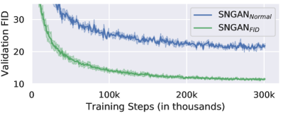
Figure 1: SNGAN trained normally (SNGAN${}_{\text{Normal}}$) and SNGAN with FID as an additional loss (SNGAN${}_{\text{FID}}$). Lower FID is better.

The improvements to FID raise an important question: Can optimization of FID as a loss “improve” generated images?

To answer this question, we take a pretrained BigGAN (Brock et al., 2019) and train it to improve FID while inspecting the generated samples. We find that several samples improve with the addition of features like ears, eyes or tongues. For example, one image of “a dog without a head” turns into an image of “a dog with a head,” see Figure 2. Such examples demonstrate that training a generator to improve FID can lead to better generated samples. We present an analysis of FID as a loss function, which may explain the observed improvements (Section 4).

In conclusion, our work allows GANs to use FID as a loss, which improves FID and can improve generated images.

The remainder of this paper is organized into sections as follows. Section 2 introduces FastFID, a novel algorithm that supports fast backpropagation through FID. Section 3 demonstrates how three different GANs attain better validation FID when trained to explicitly minimize FID. Section 4 explores whether optimizing FID as a loss can “improve” generated images.

CODE: code.ipynb (one click to run in Google Colab).

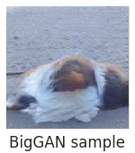
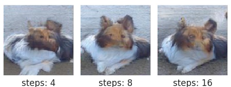
Figure 2: (Left) Fake image from pretrained BigGAN. (Right) Training BigGAN with FID improves image by “adding a head.”

2 Fast Fréchet Inception Distance

The FID between the model distribution $P_{model}$ and the real data distribution $P_{data}$ is computed as follows. Draw “fake” model samples $f_{1},...,f_{m}\sim P_{model}$ and “real” data samples $r_{1},...,r_{n}\sim P_{data}$. Encode all samples $f_{i}$ and $r_{i}$ by computing activations $A(f_{i})$ and $A(r_{i})$ of the final layer of the pretrained Inception network (Szegedy et al., 2015). Compute the sample means $\mu_{1},\mu_{2}$ and the sample covariance matrices $\Sigma_{1},\Sigma_{2}$ of the activations $A(f_{i}),A(r_{i})$. The FID is then the Wasserstein distance (Dowson & Landau, 1982) between the two multivariate normal distributions $N(\mu_{1},\Sigma_{1})$ and $N(\mu_{2},\Sigma_{2})$.

$$||\mu_{1}-\mu_{2}||_{2}^{2}+\text{tr}(\Sigma_{1})+\text{tr}(\Sigma_{2})-2\cdot\text{tr}(\sqrt{\Sigma_{1}\Sigma_{2}}).$$ (1)

For evaluation during training, the original implementation use $10000$ samples by default (Heusel et al., 2017). On our workstation, this causes the FID evaluation to take approximately $20s$. Of the $20s$, it takes approximately $10s$ to compute Inception encodings and approximately $10s$ to compute $\text{tr}(\sqrt{\Sigma_{1}\Sigma_{2}})$.

The real data samples $r_{1},...,r_{n}$ does not change during training, so we only need to compute their Inception encodings once. The $10s$ spent computing the Inception encodings is only the time it takes to encode the fake model samples $f_{1},...,f_{m}$. It is thus sufficient to reduce the number of fake samples $m$ to reduce the time spent computing Inception encodings. For example, if we reduce $m$ from $10000$ to $128$ we reduce the time spent computing Inception encodings from $10s$ to $0.1s$.

However, computing $\text{tr}(\sqrt{\Sigma_{1}\Sigma_{2}})$ still takes $10s$. FastFID mitigates this issue by efficiently computing $\text{tr}(\sqrt{\Sigma_{1}\Sigma_{2}})$ without explicitly computing $\sqrt{\Sigma_{1}\Sigma_{2}}$. Section 2.1 outlines how previous work computed $\sqrt{\Sigma_{1}\Sigma_{2}}$ and Section 2.2 explains how FastFID computes $\text{tr}(\sqrt{\Sigma_{1}\Sigma_{2}})$ efficiently.

2.1 Previous Algorithm

The original FID implementation (Heusel et al., 2017) computes $\text{tr}(\sqrt{\Sigma_{1}\Sigma_{2}})$ by first constructing $\sqrt{\Sigma_{1}\Sigma_{2}}$. The matrix square root is then computed using scipy.linalg.sqrtm  (Virtanen et al., 2020) which implements an extension of the algorithm from (Björck & Hammarling, 1983) which is rich in matrix-matrix operations (Deadman et al., 2012). The algorithm starts by computing a Schur decomposition:

$$\Sigma_{1}\Sigma_{2}=QVQ^{T}\text{ with }Q^{T}=Q^{-1}\text{and triangular }V.$$ (2)

The algorithm then computes a triangular matrix $U$ such that $U^{2}=V$ by using the triangular structure of $U$ and $V$.

In particular, the triangular structure implies the following triangular equations $U_{ii}^{2}=V_{ii}$ and $U_{ii}U_{ij}+U_{ij}U_{jj}=V_{ij}-\sum_{k=i+1}^{j-1}U_{ik}U_{kj}$ (Deadman et al., 2012). The equations can be solved wrt. $U$ one superdiagonal at a time. The resulting $U$ yields a matrix square root of the initial matrix.

$$\sqrt{\Sigma_{1}\Sigma_{2}}=QUQ^{T}.$$ (3)

Time Complexity.

Computing the Schur decomposition of $\Sigma_{1}\Sigma_{2}\in\mathbb{R}^{d\times d}$ takes $O(d^{3})$ time. The resulting triangular equations can then be solved wrt. $U$ in $O(d^{3})$ time. Computing the matrix square root thus takes $O(d^{3})$ time. FID uses the Inception network which has $d=2048$. There exists other “Fréchet-like” distances, e.g. the Fréchet ChemNet Distance (Preuer et al., 2018) which uses the ChemNet network with $d=512$. On our workstation, the different values of $d$ cause the square root computations to take approximately $10s$ for FID and $1s$ for FCD.

Uniqueness.

The matrix square root $\sqrt{M}$ is defined to be any matrix that satisfies $\sqrt{M}\sqrt{M}=M$. The square root of a matrix is in general not unique, i.e., some matrices have many square roots. The above algorithm does not necessarily find the same square root matrix if it is run several times, because the Schur decomposition is not unique. Furthermore, when computing $U_{ii}=\sqrt{T_{ii}}$ one has the freedom to choose both $\pm|\sqrt{T_{ii}}|$. The scipy.linalg.sqrtm  implementation chooses $U_{ii}=|\sqrt{T_{ii}}|$. Our implementation of the algorithm, presented in Section 2.2, computes the trace $\text{tr}(\sqrt{\Sigma_{1}\Sigma_{2}})$ such that it agrees with scipy.linalg.sqrtm  up to numerical errors.

2.2 Our algorithm

This subsection presents an algorithm that computes $\text{tr}(\sqrt{\Sigma_{1}\Sigma_{2})}$ fast. The high-level idea: construct a “small” matrix $M$ such that the eigenvalues $\lambda_{i}(M)$ satisfy $\sum_{i}|\sqrt{\lambda_{i}(M)}|=\text{tr}(\sqrt{\Sigma_{1}\Sigma_{2}})$. Since $M$ is “small,” we can compute its eigenvalues faster than we can compute the matrix square root $\sqrt{\Sigma_{1}\Sigma_{2}}$.

Let $X_{1}\in\mathbb{R}^{d\times m}$ have columns $A(f_{1}),...,A(f_{m})$ and let $X_{2}\in\mathbb{R}^{d\times n}$ have columns $A(r_{1}),...,A(r_{n})$. Let $\mathbb{1}_{k}$ be the $1\times k$ all ones vector. The sample covariance matrices $\Sigma_{1}$ and $\Sigma_{2}$ can then be computed as follows:

$$\Sigma_{i}=C_{i}C_{i}^{T}\quad\text{where} \quad C_{1}=\frac{1}{\sqrt{m-1}}(X_{1}-\mu_{1}\mathbb{1}_{m})$$ (4)

and $$\quad C_{2}=\frac{1}{\sqrt{n-1}}(X_{2}-\mu_{2}\mathbb{1}_{n}).$$ (5)

This allows us to write $\Sigma_{1}\Sigma_{2}=C_{1}C_{1}^{T}C_{2}C_{2}^{T}$. Recall that the eigenvalues of $AB$ are equal to the eigenvalues of $BA$ if both $AB$ and $BA$ are square matrices (Nakatsukasa, 2019).

The eigenvalues of the $d\times d$ matrix $C_{1}C_{1}^{T}C_{2}C_{2}^{T}$ are thus the same as the eigenvalues of the $m\times m$ matrix $M=C_{1}^{T}C_{2}C_{2}^{T}C_{1}$. The matrix $M$ is small in the sense that we will use $m\ll d$, for example, for FID we often use $m=128$ fake samples while $d=2048$.

We now show that $\sum_{i}|\sqrt{\lambda_{i}(M)}|=\text{tr}(\sqrt{\Sigma_{1}\Sigma_{2}})$ if $\sqrt{\Sigma_{1}\Sigma_{2}}$ is computed by scipy.linalg.sqrtm. Since $\text{tr}(\sqrt{\Sigma_{1}\Sigma_{2}})=\sum_{i}\lambda_{i}(\sqrt{\Sigma_{1}\Sigma_{2}})$ it is sufficient to show that the eigenvalues of $\sqrt{\Sigma_{1}\Sigma_{2}}$ are equal to the positive square root of the eigenvalues of $\Sigma_{1}\Sigma_{2}$. In other words: it is sufficient to show that $\lambda_{i}(\sqrt{\Sigma_{1}\Sigma_{2}})=|\sqrt{\lambda_{i}(\Sigma_{1}\Sigma_{2})}|$.

Recall that $\sqrt{\Sigma_{1}\Sigma_{2}}=QUQ^{T}$ where $\Sigma_{1}\Sigma_{2}=QVQ^{T}$, $U^{2}=V$ and $U_{ii}^{2}=V_{ii}$. Since both $U$ and $V$ are triangular they have their eigenvalues on the diagonal, which means that $\lambda_{i}(\sqrt{\Sigma_{1}\Sigma_{2}})=U_{ii}=\sqrt{V_{ii}}=\sqrt{\lambda_{i}(\Sigma_{1}\Sigma_{2})}$. Recall that scipy.linalg.sqrtm  chooses $U_{ii}=|\sqrt{V_{ii}}|$ and we get $\lambda_{i}(\sqrt{\Sigma_{1}\Sigma_{2}})=|\sqrt{\lambda_{i}(\Sigma_{1}\Sigma_{2})}|$ as wanted. Note that even though the Schur decomposition $\Sigma_{1}\Sigma_{2}=QUQ^{T}$ is not unique, $U$ will always have the eigenvalues of $\Sigma_{1}\Sigma_{2}$ on its diagonal and thus preserve the trace. Putting everything together, we realize the desired result:

$$\text{tr}(\sqrt{\Sigma_{1}\Sigma_{2}})=\sum_{i=1}^{m-1}|\sqrt{\lambda_{i}(C_{1}^{T}C_{2}C_{2}^{T}C_{1})}|.$$

For completeness, we provide pseudo-code in Algorithm 1. The algorithm can be modified to compute FCD by simply changing the Inception network to the ChemNet network.

Algorithm 1 Fast Fréchet Inception Distance

1:  Input: $f_{1},...,f_{m}\sim P_{model}$, the Inception network $\text{Net}(x)$ and precomputed $\mu_{2},C_{2}$.

2:  

3:  // Compute network activations

4:  Compute $A(f_{i})=\text{Net}(f_{i})$ and let $X_{1}$ be a matrix with columns $A(f_{1}),...,A(f_{m})$.

5:  

6:  // Compute mean.

7:  $\mu_{1}=\frac{1}{m}\sum_{i=1}^{m}(X_{1})_{i}$.

8:  

9:  // Compute trace of square root matrix.

10:  $C_{1}=\frac{1}{\sqrt{m-1}}(X_{1}-\mu_{1}\mathbb{1}_{m})$ as in Equation 4.

11:  $S=\text{library.eigenvalues}((C_{1}^{T}C_{2})(C_{2}^{T}C_{1}))$

12:  $\text{tr}(\sqrt{\Sigma_{1}\Sigma_{2}})=\sum_{i=1}^{m-1}|\sqrt{S_{i}}|$

13:  

14:  // Compute trace of both covariance matrices.

15:  $\text{tr}(\Sigma_{1})=\sum_{i=1}^{m}\text{row}_{i}(C_{1})^{T}\text{row}_{i}(C_{1})$

16:  $\text{tr}(\Sigma_{2})=\sum_{i=1}^{n}\text{row}_{i}(C_{2})^{T}\text{row}_{i}(C_{2})$

17:  

18:  return $||\mu_{1}-\mu_{2}||_{2}^{2}+\text{tr}{(\Sigma_{1})}+\text{tr}{(\Sigma_{2})}-2\cdot\text{tr}(\sqrt{\Sigma_{1}\Sigma_{2}})$

Time Complexity.

Computing $M=(C_{1}^{T}C_{2})(C_{2}^{T}C_{1})$ takes $O(mdn+m^{2}n)$ time. The eigenvalues of $M$ can be computed in $O(m^{3})$ time, giving a total time complexity of $O(mdn+m^{2}n+m^{3})$. If we use a large number of real samples $n\gg d$, we can precompute $\Sigma_{2}=C_{2}C_{2}^{T}$ and compute $M=C_{1}^{T}\Sigma_{2}C_{1}$ in $O(d^{2}m)$ time, giving a total time complexity of $O(d^{2}m+m^{3})$.

Computing Gradients.

If the network $\text{Net}(x)$ used in Algorithm 1 supports gradients with respect to its input, as the Inception network does, it is possible to compute gradients with respect to the input samples $f_{i}$. If $f_{i}$ were constructed by a generative model, one can also compute gradients wrt. the parameters of the generative model. If Algorithm 1 is implemented with automatic differentiation, e.g., through PyTorch (Paszke et al., 2019) or TensorFlow (Abadi et al., 2015), these gradients are computed automatically.

Potential Further Speed-ups.

Algorithm 1 computes $\text{tr}(\sqrt{\Sigma_{1}\Sigma_{2}})$ fast. As a result, computing $\text{tr}(\sqrt{\Sigma_{1}\Sigma_{2}})$ only takes a few percent of the total time spent by Algorithm 1. The majority of the time spent by Algorithm 1 is spent computing Inception encodings. One could compute the encodings faster by compressing (Chen et al., 2015) the Inception network, at the cost of introducing some small error.

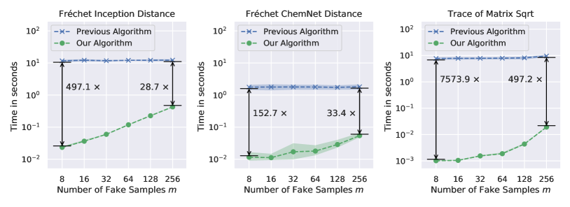
Figure 3: Comparison of scipy.linalg.sqrtm  and Algorithm 1 for different batch sizes. Left: Time to compute Fréchet Inception Distance. Middle: Time to compute Fréchet ChemNet Distance. Right: Time to compute the trace of matrix square root.

2.3 Experimental Speed-Up

In this subsection, we compare the running time of Algorithm 1 implemented in PyTorch (Paszke et al., 2019) against open-source implementations of FID, FCD and $\sqrt{\Sigma_{1}\Sigma_{2}}$. The algorithms are compared as the number of different fake samples varies $m=8,16,\dots,256$.

We used images from CelebA (Liu et al., 2015) to time FID. We used molecules from MOSES (Polykovskiy et al., 2018) to time FCD. For both FID and FCD, we precomputed $\Sigma_{2}$ with $10000$ real samples.

To time $\text{tr}(\sqrt{C_{1}^{T}\Sigma_{2}C_{1}})$, we used $\Sigma_{2}\in\mathbb{R}^{d\times d}$ with $N(0,1)$ entries. We computed $C_{1}$ by using Equation 4 where $X_{1}\in\mathbb{R}^{d\times m}$ had $N(0,1)$ entries. To make the timing of $\text{tr}(\sqrt{C_{1}^{T}\Sigma_{2}C_{1}})$ comparable with FID, we chose $d=2048$ to match the Inception network.

For each $m$, we ran one warmup round and then repeated the experiment $100$ times. Figure 3 plots average running time with standard deviation as error bars.

The previous algorithms take roughly the same amount of time for all $m$. This is expected since most of the time is spent computing $\sqrt{\Sigma_{1}\Sigma_{2}}$, which takes the same amount of time for all $m$. Our algorithm takes less time as $m$ decreases. This is expected since our algorithm takes $O(m^{3}+d^{2}m)$ time for precomputed $\Sigma_{2}$.

For all $m$, our algorithm is at least $25$ times faster than the previous algorithms, and in some cases up to hundreds or even thousands of times faster. Notably, both algorithms computed the same thing, our algorithm just computed the same thing faster. To concretize the reduction in training time, we exemplify the reduction below.

Example.

Section 3 trains GANs to minimize FID with batch size $m=128$. Our algorithm then reduces computation time from $12.15\pm 0.80$ seconds to $0.23\pm 0.01$ seconds (mean $\pm$ standard deviation). When training for $10^{5}$ steps (as done in Section 3) this reduces time by 13 days. When training for $10^{6}$ steps (as done in (Zhang et al., 2019)) this reduces time by 130 days.

2.4 Numerical Error

To investigate the numerical error of Algorithm 1 and scipy.linalg.sqrtm, we ran an experiment where the square root can easily be computed. If we choose $C_{1}=C_{2}$ then $C_{1}C_{1}^{T}C_{2}C_{2}^{T}=(C_{1}C_{1}^{T})^{2}$ is positive semi-definite and has a unique positive semi-definite square root $\sqrt{(C_{1}C_{1}^{T})^{2}}=C_{1}C_{1}^{T}$. Furthermore, it is exactly this positive semi-definite square root scipy.linalg.sqrtm computes since the implementation chooses the positive eigenvalues $U_{ii}=|\sqrt{V_{ii}}|$ (see Section 2.1 for details). We can then investigate the numerical errors by comparing the ground truth $\text{tr}(C_{1}C_{1}^{T})$ with the result from both Algorithm 1 and scipy.linalg.sqrtm.

The experiment was repeated for $m=32,64,128,256$ number of fake samples, where $C_{1}$ was computed as done in Section 2.3. We report the ground truth $\text{tr}(C_{1}C_{1}^{T})$ and the absolute numerical error caused by Algorithm 1 and scipy.linalg.sqrtm:

$$\left|\text{tr}(C_{1}C_{1}^{T})-\text{tr}(\textsc{scipy.sqrtm}(C_{1}C_{1}^{T}C_{1}C_{1}^{T}))\right|.$$ (6)

See results in Table 1.

$m$	Answer	Error scipy	Error Algorithm 1
8	14283	175	0.0000
16	30678	228	0.0020
32	62955	300	0.0000
64	128947	408	0.0078
128	259586	565	0.0156
256	523360	785	0.0312

Table 1: Numerical error of scipy.sqrtm and Algorithm 1 for different number of fake samples $m$. We also add correct answer so the percentage wise numerical error can be inferred.

The numerical error of Algorithm 1 is at least $1000$ times smaller than that of scipy.linalg.sqrtm. We suspect that Algorithm 1 has smaller numerical errors because it computes eigenvalues of a “small” $m\times m$ matrix instead of computing a Schur decomposition of the “full” $d\times d$ matrix.

The above experiment used 32 bit precision. By default, scipy.linalg.sqrtm  uses 64 bit precision and exhibit negligible numerical errors. Neural networks are usually trained with 32 bit precision and sometimes even 16 bit precision. Additional numerical stability is thus desirable as it allows us to reduce numerical precision.

3 Training GANs with FID as a Loss

This section demonstrates that GANs trained with FID as an additional loss get better validation FID. Experimental setup: we find an open-source implementation of a popular GAN, and train it while monitoring validation FID. We then train an identical GAN, but with FID as an additional loss. The experiment is repeated 3 times and we report $\mu\pm\sigma$ where $\mu$ is the mean validation FID and $\sigma$ is the standard deviation. For each repetition, we show 8 fake samples (see appendix in the supplementary material for enlarged images).

To increase the robustness of our experiment, we performed the experiment with three different GANs on three different datasets. SNGAN (Miyato et al., 2018) on CIFAR10 (Krizhevsky, 2009), DCGAN (Radford et al., 2016) on CelebA (Liu et al., 2015) and SAGAN (Zhang et al., 2019) on ImageNet (Deng et al., 2009). To distinguish between GANs with and without FID loss we write, e.g., SNGAN${}_{\text{FID}}$ and SNGAN${}_{\text{}}$, respectively.

SNGAN on CIFAR10. We train SNGAN on CIFAR10. After 301070 training steps validation FID improved from $21.81\pm 0.73$ to $11.48\pm 0.22$. See Figure 6 for validation FID during training. Below the plot we include fake images from SAGAN${}_{\text{}}$ (left) and fake images from SAGAN${}_{\text{FID}}$ (right), each row corresponds to one repetition of the experiment.

To add context, BigGAN and SAGAN got FID $14.73$ and $13.4$, respectively (Tran et al., 2019). Both SAGAN and BigGAN were published after SNGAN, and introduced improvements to both architecture and training. From this perspective, it is interesting that SNGAN can beat both SAGAN and BigGAN by simply adding FID to the loss function. State-of-the-art is 7.01 (Karras et al., 2020).

DCGAN on CelebA. We train DCGAN on CelebA at 64x64 resolution. After 100264 training steps validation FID improved from $15.67\pm 1.38$ to $11.03\pm 0.43$. Figure 6 contains validation FID and samples like Figure 6.

SAGAN on ImageNet. We train SAGAN on ImageNet at 128x128 resolution. After 100001 training steps validation FID improved from $129.48\pm 2.38$ to $97.64\pm 4.33$. Figure 6 contains validation FID and samples like Figure 6.

Experimental Conclusion. The generators that use FID as an additional loss get better validation FID in all experiments. This raises an important question: Can optimization of FID as a loss “improve” generated images?

We address this question in Section 4. The remainder of this section, Section 3.1, presents further details regarding the experiments described in this section.

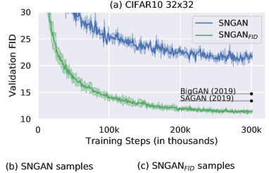
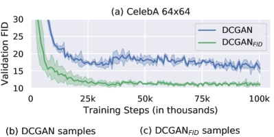
Figure 4: SNGAN trained on CIFAR10. (a) validation FID (b) fake samples from SNGAN${}_{\text{}}$ (c) fake samples from SNGAN${}_{\text{FID}}$.

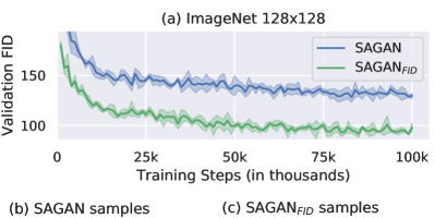
Figure 5: DCGAN trained on CelebA. (a) validation FID (b) fake samples from DCGAN${}_{\text{}}$ (c) fake samples from DCGAN${}_{\text{FID}}$.

Figure 6: SAGAN trained on ImageNet. (a) validation FID (b) fake samples from SAGAN${}_{\text{}}$ (c) fake samples from SAGAN${}_{\text{FID}}$.

3.1 Experimental Details

Training.

GANs have two neural networks, a generator $G$ and a discriminator $D$. The generator is trained to make fake samples $F$ that minimize the discriminator loss $L_{\text{D}}(F)$,

$$\min L_{\text{D}}(F).$$ (7)

The generator is often evaluated by computing FID between $10^{4}$ real images $X$ and $10^{4}$ fake images $F$,

$$\text{FID}(X,F).$$ (8)

We add FID to the generators loss,

$$\min L_{\text{D}}(F)+\text{FID}(X,F).$$ (9)

The generators then jointly minimize $L_{\text{D}}$ and FID. In all experiments, we optimized the joint loss function using gradient descent with a mini-batch of 128 fake examples. Notably, FastFID allows us to efficiently compute FID between the entire training data $X$ and a mini-batch of fake samples. In turn, we do not sample a mini-batch from the training data, which removes variance caused by sampling.

The authors of FID suggest evaluating FID with at least $10^{4}$ fake samples (FID${}_{10^{4}}$). One might therefore be concerned that a mini-batch with $128$ fake samples (FID₁₂₈) is insufficient for training. In all three experiments, we saw training to minimize FID₁₂₈ consistently yielded smaller FID${}_{10^{4}}$. This leads us to conclude a batch size of $128$ fake samples is sufficient when FID is used for training.

Scaling Loss.

The discriminator loss $L_{\text{D}}$ usually lies within $[-10,10]$, much smaller than FID₁₂₈, which typically lies within $[0,500]$. This causes the gradients from FID₁₂₈ to be up to $50\times$ larger than the gradients from $L_{\text{D}}$, which subsequently breaks training. We circumvented this issue by adaptively scaling FID to match the discriminator loss $L_{\text{D}}$.

$$\text{scaled loss}=L_{\text{D}}+\text{FID}\;/\underbrace{\text{FID}\cdot L_{\text{D}}}_{\text{without gradients}}$$ (10)

Training SAGAN was initially unstable, we found that further dividing the FID loss by 2 improved training stability.

Computing FID.

FID is computed differently by PyTorch (Paszke et al., 2019) and TensorFlow (Abadi et al., 2015). This is caused by architectural differences in the implementation of the Inception network, e.g., TensorFlow uses mean pooling while PyTorch use max pooling. These issues were fixed in an implementation by (Seitzer, 2020), which we use to compute FID in the SNGAN and SAGAN experiment. To test whether the observed improvements were dependent to the specifics of the Inception architecture, we used the following PyTorch implementation in the DCGAN experiments:

github.com/hukkelas/pytorch-frechet-inception-distance

Train and Validation Sets.

(Heusel et al., 2017) provide precomputed Inception statistics. On some datasets the statistics are computed on the training data, while on others, they are computed on the validation data. Since we optimize FID on training data we report FID on validation data.

GPU Memory.

The joint loss Equation 10 requires us to backpropagate through both $L_{\text{D}}$ and FID, which increases peak memory consumption. We mitigate this issue with two separate backward passes for $L_{\text{D}}$ and FID.

The open-source implementation of SAGAN used two GPUs to reach batch size 128. Due to hardware limitations, we had to fit SAGAN on a single GPU. However, SAGAN took up all 11 GB of our GPUs memory at batch size 64. To keep batch size 128 on a single GPU we used gradient checkpointing (Chen et al., 2016) and 16-bit precision.

Backpropagation and Eigenvalues.

Algorithm 1 needs to backpropagate through torch.eig(M). At the time of writing, backpropagation through torch.eig is not supported in the stable release (PyTorch v1.7.1). Since $M$ is symmetric $M=M^{T}$ one can use torch.symeig which does support backpropagation. One can also use torch.svd to compute singular values, since $M$ is positive semi-definite the eigenvalues and singular values are equal $\lambda_{i}(M)=\sigma_{i}(M)$. Alternatively, the unstable PyTorch 1.8 does support backpropagation through torch.eig.

Other Generative Models.

Normalizing Flows (NFs) (Dinh et al., 2015) are generative models with many desirable properties, however, they sometimes attain poor FID. The poor FID motivated us to train the NF called Glow (Kingma & Dhariwal, 2018) to minimize FID and negative log-likelihood. The resulting Glow produced samples with “unrealistic” artifacts, see Figure 7(a).

The artifacts raise an interesting question: why does FID training cause Glow to produce artifacts but not SNGAN${}_{\text{FID}}$? We hypothesize that the discriminator learns to detect the “unrealistic” artifacts and penalizes the generator. If this hypothesis is true, we would expect SNGAN${}_{\text{FID}}$ to produce “unrealistic” artifacts if we removed the discriminator. Indeed, if we train SNGAN${}_{\text{FID}}$ as in the previous section, but remove the discriminator after 1000 steps, the generator starts producing “unrealistic” artifacts, see Figure 7(b).

(a)
(b)

Figure 7: (a) Glow trained to minimize FID produce samples with “unrealistic” artifacts. (b) Removing the discriminator from SNGAN also leads to “unrealistic” artifacts.

4 Can FID Loss Improve Generated Images?

This section explores whether FID as a loss function can improve generated fake images. The experimental setup: we use BigGAN pretrained for $10^{5}$ iterations and train the generator to minimize FID without its discriminator. The discriminator is discarded to ensure that changes in the fake images are due to the FID loss and not the discriminator.

Goal. A generator might improve the FID loss by changing a few pixels of the generated images to fool FID. Our goal is to explore whether the FID loss leads the generator to “fool FID” or “improve the fake images.”

Observations. We track how 64 samples change during training. All samples had perceptible changes ruling out “few pixel changes” (see supplementary material). We comment on two insightful samples below, which both demonstrate the addition of features like ears, eyes or heads.

Figure 8 contains BigGAN samples of a bird, each row corresponds to a repetition of the experiment. The left-most column shows the original bird generated by the pretrained BigGAN. The following columns demonstrate how the bird changes as FID is minimized. Notably, the initial bird lacks a beak. In all repetitions, we found that minimizing FID made the generator add a “beak”-like feature.

Figure 9 contains samples of a dog, where the initial dog has no head. In all repetitions, we found that minimizing FID made the generator add features like ears, eyes or heads.

Conclusion. FID minimization can improve the fake images with the addition of features like ears, eyes or heads. This demonstrates that FID minimization does not necessarily lead the generator to “fool FID” and can (in some cases) “improve the fake images.”

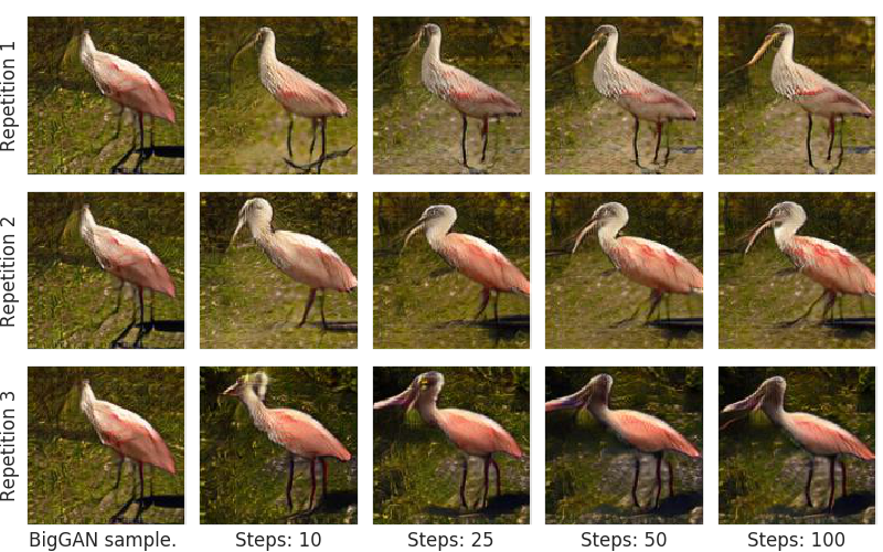
Figure 8: Visualization of changes to samples while FID is minimized. Each row corresponds to a repetition of the experiment. Each column shows samples after a given number of steps.

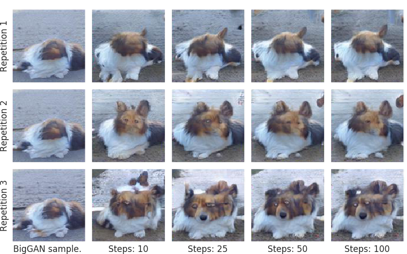
Figure 9: Visualization of changes to samples while FID is minimized. Each row corresponds to a repetition of the experiment. Each column shows samples after a given number of steps.

CODE: code.ipynb (one click to run in Google Colab).

4.1 Further details

Understanding FID.

Some of the dogs in Figure 9 have two heads. Such behavior might be explained by carefully inspecting the FID equation.

$$\underbrace{||\mu_{1}-\mu_{2}||_{2}^{2}}_{\text{mean difference }\Delta_{\mu}}+\underbrace{\text{tr}(\Sigma_{1})+\text{tr}(\Sigma_{2})-2\text{tr}(\sqrt{\Sigma_{1}\Sigma_{2}})}_{\text{covariance difference }\Delta_{\Sigma}}.$$ (11)

The term $\Delta_{\mu}$ penalizes the differences between the average Inception activations of the real data and the fake data. Suppose the entry $\mu_{1}^{\text{head}}$ and the entry $\mu_{2}^{\text{head}}$ contain the average number of heads detected by the Inception network.  Then $(\mu_{1}^{\text{head}}-\mu_{2}^{\text{head}})^{2}$ measures a difference in the average number of heads detected between the fake and real data. If the average number of heads in the fake data $\mu_{1}^{\text{head}}$ is smaller than the average number for the real data $\mu_{2}^{\text{head}}$, then $\Delta_{\mu}$ may encourage the generator to produce more heads. Notably, $\Delta_{\mu}$ might be indifferent to whether the heads are attached to a single dog.

The term $\Delta_{\Sigma}$ penalizes the differences between the covariance of Inception activations of the real data and the fake data. Suppose the entry $\mu_{i}^{\text{eye}}$ contains the average number of eyes detected by the Inception network. Then, $\Sigma_{i}^{\text{head, eye}}$ would measure the co-variance of heads and eyes.

Altogether, it seems that FID incentivizes the generator to generate images where features (like heads and eyes) occur and co-occur in the same way as in training data. We hypothesize this incentive is the reason why the FID loss can improve the generated samples.

Experimental Notes.

The BigGAN model was pretrained for $10^{5}$ iterations with batch size 2048 using 8 GPUs (Tesla V100) for a total of 128 GB memory. We had access to a single Tesla P100 with 16 GB memory through Google Colab: www.colab.research.google.com.

To fit everything on a single 16 GB GPU, we used gradient checkpointing and half-precision training as in Section 3.1. Furthermore, we accumulated gradients from batches of size 100 over 10 iterations to reach a total batch size of 1000. This still reduced the batch size from 2048 to 1000, which we corrected for by dividing the learning rate by two.

To stabilize training, we fixed the latent vectors and only optimize the first two layers of the generator. Note that it is easier for the generator to “fool FID” for a fixed set of latent vectors instead of $z\sim N(0,I)$ because it can take all values in $\mathbb{R}^{d}$.

5 Related Work

The literature contains several methods for evaluating generative models. An overview can be found in (Borji, 2019) which reviews a total of 29 different methods. This article concerns FID, which has arguably become the standard for benchmarking generative models in computer vision.

5.1 Fréchet Inception Distance

(Heusel et al., 2017) introduced FID and demonstrated that FID is consistent with increasing levels of disturbances and human judgment. To justify FID, the authors assume that the Inception activations are normally distributed. Whether this assumption holds or not, does not change the fact that the computed FID was consistent with increased levels of disturbances and human judgment.

The authors provide precomputed Inception statistics for five datasets. Some use validation sets and others do not. This has, understandably, caused a bit of confusion, with some work reporting training FID and others reporting validation FID. We report validation FID since we explicitly optimize training FID.

The authors state “The number of samples should be greater than 2048. Otherwise $\Sigma$ is not full rank resulting in complex numbers and NaNs by calculating the square root.” We compute $\text{tr}(\sqrt{\Sigma})$ directly without explicitly computing $\sqrt{\Sigma}$, which works even when $\Sigma$ has low rank. Our algorithm even becomes faster when the rank of $\Sigma$ decreases.

To the best of our knowledge, no previous work use FID as a loss function. We suspect the main obstacle preventing this in prior work has been the slow computation of FID, an issue FastFID mitigates.

5.2 Faster FID Computations

To the best of our knowledge, there exist no published articles which reduce the asymptotic time complexity of FID. However, one implementation contains a few tricks. In this implementation, the function at line 525 reduces the time complexity from $O(d^{3}+d^{2}m)$ to $O(dm)$ by computing only $||\mu_{1}-\mu_{2}||_{2}^{2}$, omitting the trace term $\text{tr}(\Sigma_{1}+\Sigma_{2}-2\sqrt{\Sigma_{1}\Sigma_{2}})$. Another function at line 582 incorporates the covariance matrices while retaining the $O(dm)$ time complexity, by only using the diagonal entries of the covariance matrices. Yet another function at line 411 computes $\text{tr}(\sqrt{\Sigma_{1}\Sigma_{2}})$ by computing an eigendecomposition of two related matrices. Their derivations have some similarities to our derivations, but they do not exploit low rank (small $m$) and take $O(d^{3}+d^{2}m)$ time instead of $O(d^{2}m+m^{3})$. That said, eigendecompositions can be used to improve the baseline in Section 2.2 by a constant factor. Relative to such an improved baseline, in the example of Section 2.3, FastFID will remove roughly $13$ days of “wasted” computation instead of $130$ days.

(Lin & Maji, 2017) present an algorithm that approximates a matrix square root, which is much faster than scipy.linalg.sqrtm. Notably, this approximation is used in the open-source implementations of BigGAN to provide a fast FID approximation.

The above algorithms all differ from FastFID, by either approximating FID, computing something entirely different or having an $O(d^{3}+d^{2}m)$ time complexity.

6 Conclusion

Computing gradients through FID with automatic differentiation can increase training time by many days. FastFID computes the needed gradients efficiently by utilizing eigenvalue considerations. This allows us to use FastFID to train GANs with FID as a loss function. Such training consistently improves the validation FID for different GANs on different datasets. We attempt to investigate whether FID as a loss encourages the generator to “fool FID” or generate better images. We find some evidence that suggests FID as a loss function can improve the samples of a generator, however, understanding when this happens and when it does not remains unclear, and should be the focus of further research.

Remark.

FID can now be optimized directly. To allow fair comparisons in future research, we recommend future researchers explicitly denote whenever a generative model explicitly optimize FID, e.g., SNGAN${}_{\text{FID}}$ or SNGAN${}^{\text{FID}}$.

SNGAN${}_{\text{}}$

SNGAN${}_{\text{FID}}$

Figure 10: Bigger version of samples in Figure 6.

DCGAN${}_{\text{}}$

DCGAN${}_{\text{FID}}$

Figure 11: Bigger version of samples in Figure 6.

SAGAN${}_{\text{}}$

SAGAN${}_{\text{FID}}$

Figure 12: Bigger version of samples in Figure 6.

References

- Abadi et al. (2015) Abadi, M., Agarwal, A., Barham, P., Brevdo, E., Chen, Z., Citro, C., Corrado, G. S., Davis, A., Dean, J., Devin, M., Ghemawat, S., Goodfellow, I., Harp, A., Irving, G., Isard, M., Jia, Y., Jozefowicz, R., Kaiser, L., Kudlur, M., Levenberg, J., Mané, D., Monga, R., Moore, S., Murray, D., Olah, C., Schuster, M., Shlens, J., Steiner, B., Sutskever, I., Talwar, K., Tucker, P., Vanhoucke, V., Vasudevan, V., Viégas, F., Vinyals, O., Warden, P., Wattenberg, M., Wicke, M., Yu, Y., and Zheng, X. TensorFlow: Large-Scale Machine Learning on Heterogeneous Systems, 2015. URL http://tensorflow.org/. Software available from tensorflow.org.
- Björck & Hammarling (1983) Björck, Å. and Hammarling, S. A Schur Method for the Square Root of a Matrix. Linear algebra and its applications, 1983.
- Borji (2019) Borji, A. Pros and Cons of GAN Evaluation Measures. Computer Vision and Image Understanding, 179:41–65, 2019.
- Brock et al. (2019) Brock, A., Donahue, J., and Simonyan, K. Large Scale GAN Training for High Fidelity Natural Image Synthesis. In International Conference on Learning Representations, 2019. URL https://openreview.net/forum?id=B1xsqj09Fm.
- Chen et al. (2016) Chen, T., Xu, B., Zhang, C., and Guestrin, C. Training Deep Nets with Sublinear Memory Cost. abs/1604.06174, 2016.
- Chen et al. (2015) Chen, W., Wilson, J., Tyree, S., Weinberger, K., and Chen, Y. Compressing Neural Networks with the Hashing Trick. In International conference on machine learning, pp. 2285–2294, 2015.
- Deadman et al. (2012) Deadman, E., Higham, N. J., and Ralha, R. Blocked Schur Algorithms for Computing the Matrix Square Root. In International Workshop on Applied Parallel Computing, pp. 171–182. Springer, 2012.
- Deng et al. (2009) Deng, J., Dong, W., Socher, R., Li, L.-J., Li, K., and Fei-Fei, L. ImageNet: A Large-Scale Hierarchical Image Database. In CVPR09, 2009.
- Dinh et al. (2015) Dinh, L., Krueger, D., and Bengio, Y. NICE: Non-Linear Independent Components Estimation. In ICLR (Workshop), 2015.
- Dowson & Landau (1982) Dowson, D. and Landau, B. The Fréchet Distance between Multivariate Normal Distributions. Journal of multivariate analysis, 1982.
- Goodfellow et al. (2014) Goodfellow, I., Pouget-Abadie, J., Mirza, M., Xu, B., Warde-Farley, D., Ozair, S., Courville, A., and Bengio, Y. Generative Adversarial Nets. In NIPS, 2014.
- Heusel et al. (2017) Heusel, M., Ramsauer, H., Unterthiner, T., Nessler, B., and Hochreiter, S. GANs Trained by a Two Time-Scale Update Rule Converge to a Local Nash Equilibrium. In Advances in neural information processing systems, pp. 6626–6637, 2017.
- Karras et al. (2020) Karras, T., Aittala, M., Hellsten, J., Laine, S., Lehtinen, J., and Aila, T. Training Generative Adversarial Networks with Limited Data. NeurIPS, 2020.
- Kingma & Dhariwal (2018) Kingma, D. P. and Dhariwal, P. Glow: Generative Flow with Invertible 1x1 Convolutions. In NeurIPS, 2018.
- Krizhevsky (2009) Krizhevsky, A. Learning Multiple Layers of Features From Tiny Images. Technical report, 2009.
- Lin & Maji (2017) Lin, T.-Y. and Maji, S. Improved Bilinear Pooling with CNNs. In British Machine Vision Conference (BMVC), 2017.
- Liu et al. (2015) Liu, Z., Luo, P., Wang, X., and Tang, X. Deep Learning Face Attributes in the Wild. In Proceedings of International Conference on Computer Vision (ICCV), December 2015.
- Miyato et al. (2018) Miyato, T., Kataoka, T., Koyama, M., and Yoshida, Y. Spectral Normalization for Generative Adversarial Networks. In ICLR, 2018.
- Mordvintsev et al. (2015) Mordvintsev, A., Olah, C., and Tyka, M. Inceptionism: Going Deeper into Neural Networks, 2015.
- Nakatsukasa (2019) Nakatsukasa, Y. The Low-Rank Eigenvalue Problem, 2019.
- Paszke et al. (2019) Paszke, A., Gross, S., Massa, F., Lerer, A., Bradbury, J., Chanan, G., Killeen, T., Lin, Z., Gimelshein, N., Antiga, L., Desmaison, A., Kopf, A., Yang, E., DeVito, Z., Raison, M., Tejani, A., Chilamkurthy, S., Steiner, B., Fang, L., Bai, J., and Chintala, S. Pytorch: An Imperative Style, High-Performance Deep Learning Library. In NeurIPS, 2019.
- Polykovskiy et al. (2018) Polykovskiy, D., Zhebrak, A., Sanchez-Lengeling, B., Golovanov, S., Tatanov, O., Belyaev, S., Kurbanov, R., Artamonov, A., Aladinskiy, V., Veselov, M., Kadurin, A., Nikolenko, S., Aspuru-Guzik, A., and Zhavoronkov, A. Molecular Sets (MOSES): A Benchmarking Platform for Molecular Generation Models. arXiv preprint arXiv:1811.12823, 2018.
- Preuer et al. (2018) Preuer, K., Renz, P., Unterthiner, T., Hochreiter, S., and Klambauer, G. Fréchet ChemNet Distance: a Metric for Generative Models for Molecules in Drug Discovery. Journal of chemical information and modeling, 58(9):1736–1741, 2018.
- Radford et al. (2016) Radford, A., Metz, L., and Chintala, S. Unsupervised Representation Learning with Deep Convolutional Generative Adversarial Networks. In 4th International Conference on Learning Representations, ICLR, 2016.
- Seitzer (2020) Seitzer, M. PyTorch-FID: FID Score for PyTorch. https://github.com/mseitzer/pytorch-fid, August 2020. Version 0.1.1.
- Szegedy et al. (2015) Szegedy, C., Liu, W., Jia, Y., Sermanet, P., Reed, S., Anguelov, D., Erhan, D., Vanhoucke, V., and Rabinovich, A. Going Deeper with Convolutions. In Proceedings of the IEEE conference on computer vision and pattern recognition, 2015.
- Tran et al. (2019) Tran, N.-T., Tran, V.-H., Nguyen, N.-B., Yang, L., and Cheung, N.-M. Self-Supervised GAN: Analysis and Improvement With Multi-Class MiniMax Game. NeurIPS, 2019.
- Virtanen et al. (2020) Virtanen, P., Gommers, R., Oliphant, T. E., Haberland, M., Reddy, T., Cournapeau, D., Burovski, E., Peterson, P., Weckesser, W., Bright, J., van der Walt, S. J., Brett, M., Wilson, J., Jarrod Millman, K., Mayorov, N., Nelson, A. R. J., Jones, E., Kern, R., Larson, E., Carey, C., Polat, İ., Feng, Y., Moore, E. W., Vand erPlas, J., Laxalde, D., Perktold, J., Cimrman, R., Henriksen, I., Quintero, E. A., Harris, C. R., Archibald, A. M., Ribeiro, A. H., Pedregosa, F., van Mulbregt, P., and Contributors, S. . . SciPy 1.0: Fundamental Algorithms for Scientific Computing in Python. Nature Methods, 2020.
- Zhang et al. (2019) Zhang, H., Goodfellow, I., Metaxas, D., and Odena, A. Self-Attention Generative Adversarial Networks. In ICML, 2019.
SNGAN
SNGAN
DCGAN
DCGAN
SAGAN
SAGAN