$\theta$-dependence in the small-$N$ limit of $2d$ $CP^{N-1}$ models

Abstract

We present a systematic numerical study of $\theta$-dependence around $\theta=0$ in the small-$N$ limit of $2d$ $CP^{N-1}$ models, aimed at clarifying the possible presence of a divergent topological susceptibility in the continuum limit. We follow a twofold strategy, based on one side on direct simulations for $N=2$ and $N=3$ on lattices with correlation lengths up to $O(10^{2})$, and on the other side on the small-$N$ extrapolation of results obtained for $N$ up to $9$. Based on that, we provide conclusive evidence for a finite topological susceptibility at $N=3$, with a continuum estimate $\xi^{2}\chi=0.110(5)$. On the other hand, results obtained for $N=2$ are still inconclusive: they are consistent with a logarithmically divergent continuum extrapolation, but do not yet exclude a finite continuum value, $\xi^{2}\chi\sim 0.4$, with the divergence taking place for $N$ slightly below 2 in this case. Finally, results obtained for the non-quadratic part of $\theta$-dependence, in particular for the so-called $b_{2}$ coefficient, are consistent with a $\theta$-dependence matching that of the Dilute Instanton Gas Approximation at the point where $\xi^{2}\chi$ diverges.

1 Introduction

The $CP^{N-1}$ models in two space-time dimensions have been extensively studied in the literature because they represent an interesting theoretical laboratory for the study of gauge theories D’Adda et al. (1978); Shifman (2012); Vicari and Panagopoulos (2009). As a matter of fact, many intriguing non-perturbative properties, such as confinement, the existence of field configurations with non-trivial topology and the related $\theta$-dependence are features that these models share with $4d$ Yang-Mills theories.

The Euclidean action of these models, including the topological term, can be written through a non-propagating Abelian field $A_{\mu}$ as

$$S(\theta)=\int d^{2}x\left[\frac{N}{g}\bar{D}_{\mu}\bar{z}(x)D_{\mu}z(x)-i\theta q(x)\right],$$ (1)

where $N$ is the number of components of the complex scalar field $z$, which is subject to the constraint $\bar{z}z=1$, $D_{\mu}=\partial_{\mu}+iA_{\mu}$ and

$$Q=\int d^{2}x\,q(x)=\frac{1}{2\pi}\epsilon_{\mu\nu}\int d^{2}x\,\partial_{\mu}A_{\nu}(x)$$ (2)

is the topological charge. The $\theta$-dependent vacuum energy (density) is defined through the path integral as

$$E(\theta)=-\frac{\log Z(\theta)}{V}=-\frac{1}{V}\log\int[d\bar{z}][dz][dA]e^{-S(\theta)}$$ (3)

and it can be parametrized in terms of the cumulants $\braket{Q^{n}}_{c}$ of the topological charge distribution at $\theta=0$ $P(Q)$ as:

$$f(\theta)\equiv E(\theta)-E(0)=\frac{1}{2}\chi\theta^{2}\left(1+\sum_{n=1}^{\infty}b_{2n}\theta^{2n}\right),$$ (4)

where the topological susceptibility

$$\chi\equiv\frac{\braket{Q^{2}}_{c}}{V}\bigg{|}_{\theta=0}=\frac{\braket{Q^{2}}}{V}\bigg{|}_{\theta=0}$$ (5)

parametrizes the leading $\theta^{2}$ term while the coefficients

$$b_{2n}\equiv(-1)^{n}\frac{2}{(2n+2)!}\frac{\braket{Q^{2n+2}}_{c}}{\braket{Q^{2}}}\bigg{|}_{\theta=0}$$ (6)

parametrize the non-quadratic part.

One of the most interesting features of the $CP^{N-1}$ models is the possibility of performing a systematic expansion of any observable, including those related to $\theta$-dependence, in the inverse of the number of field components $1/N$ when $N\to\infty$ while $g$ is kept fixed D’Adda et al. (1978); that closely resembles the $1/N$ expansion of $4d$ $SU(N)$ gauge theories for large number of colors. The similarities are non-trivial, since the relevant scaling quantity turns out to be $\theta/N$ in both cases Witten (1980, 1998); Rossi (2016); Bonati et al. (2016a), leading to the prediction that the quantities $\bar{b}_{2n}\equiv N^{2n}b_{2n}$ are finite in the large-$N$ limit: this scaling behavior has been verified by numerical lattice simulations both for the $CP^{N-1}$ Bonati et al. (2016a); Berni et al. (2019) and for $SU(N)$ gauge theories Del Debbio et al. (2006); Bonati et al. (2016a) up to the quartic coefficient $b_{2}$. From a quantitative point of view, $CP^{N-1}$ models are more predictive, since the leading term in the $1/N$ expansion is known D’Adda et al. (1978); Del Debbio et al. (2006); Rossi (2016); Bonati et al. (2016a) for all coefficients in the $\theta$-expansion of the free energy in Eq. (4), and also the first subleading term in the case of the topological susceptibility Campostrini and Rossi (1991), while in the case of $4d$ $SU(N)$ gauge theories one has just phenomenological predictions, based on the spectrum of pseudoscalar mesons, for the leading term in the $1/N$ expansion of the topological susceptibility Witten (1979); Veneziano (1979).

Numerical simulations underlined also some differences between the two theories. Indeed, while in the Yang-Mills case the large-$N$ expected scaling practically holds already for $N\geq 3$ Bonati et al. (2016a), this is not quite the case for the $CP^{N-1}$ models. Indeed, the large-$N$ limit of $b_{2}$ shows significant deviations from large-$N$ predictions even for $N\sim 50$, and an agreement with lattice data can be recovered only by including large higher-order corrections in $1/N$; a similar behavior is observed for the topological susceptibility Bonanno et al. (2019); Berni et al. (2019).

Another important difference emerges when looking at the small-$N$ limit. Indeed, while this is predicted and observed to be regular in the case of $4d$ $SU(N)$ gauge theories, a singular behavior is expected for $2d$ $CP^{N-1}$ approaching $N=2$. For instance, one expects a divergence of the topological susceptibility of the $CP^{1}$ theory, which can be justified in perturbation theory on the basis of the ultraviolet (UV) divergence of the instanton size distribution Jevicki (1977); Forster (1977); Berg and Lüscher (1979); Fateev et al. (1979); Richard and Rouet (1983)

$$P_{N}(\rho)\propto\rho^{N-3}$$ (7)

occurring for $N=2$. This result has been tested in many lattice studies and there seems to be a general consensus about the singular behavior of $\chi$ for $N=2$ and about its origin due to the presence of small instantons, see, e.g., Refs. D’Elia et al. (1995, 1997); Blatter et al. (1996); Ahmad et al. (2005); Lian and Thacker (2007); Bietenholz et al. (2010, 2018). However, there are still many aspects deserving a more careful investigation.

First of all, as we discuss later on, the actual verification of the divergent behavior occurring for $N=2$ requires to perform a continuum limit extrapolation which is highly non-trivial, since the divergence is expected to appear as a logarithm of the UV cutoff, i.e., of the lattice spacing $a$, which could be difficult to disentangle from a regular power-law behavior in $a$ and requires numerical results spanning over orders of magnitude in terms of the dimensionless correlation length of the system.

The second issue is that a divergent behavior for the topological susceptibility has been claimed to be observed also for $N=3$ in Ref. Lian and Thacker (2007), where the authors employed a standard lattice action along with an overlap definition of the topological charge, however this is in contradiction with previous results obtained using a different action discretization and a geometric lattice definition of $Q$ Petcher and Lüscher (1983): the origin of this discrepancy may be due to the fact that, according to Eq. (7), also for $N=3$ small instantons are expected to dominate, so that also in this case the continuum limit has to be handled with care.

Finally, one would like to understand whether the small-$N$ divergent behavior regards just the topological susceptibility or also other coefficients in the Taylor expansion of the free energy in Eq. (4). In asymptotically free theories, small size instantons are expected to be weakly interacting, so that a possible conjecture Bonanno et al. (2019) is that $\theta$-dependence in the $N=2$ limit be described by the Dilute Instanton Gas Approximation (DIGA):

$$f_{\mathit{DIGA}}(\theta)=\chi\left(1-\cos\theta\right)$$ (8)

with the divergence appearing just in $\chi$, while the $b_{2n}$ coefficients are finite and have alternate sign:

$$b_{2n}^{\mathit{DIGA}}=(-1)^{n}\frac{2}{(2n+2)!}\,.$$ (9)

It is worth stressing that this conjecture would lead, apart from the global divergent factor in front, to a smooth behavior in $\theta=\pi$, unlike what happens at large-$N$, where $f(\theta)$ is expected to have a cusp in this point. In principle, this is not in contrast with some recent theoretical results obtained for the $CP^{N-1}$ models using ’t Hooft anomaly matching Gaiotto et al. (2017); Sulejmanpasic and Tanizaki (2018). Indeed, the anomaly matching at $\theta=\pi$ constrains $CP^{N-1}$ models with $N$ even to either spontaneously break the charge conjugation symmetry (i.e., $f(\theta)$ has a cusp in $\theta=\pi$) or to behave as a conformal field theory (i.e., the dynamically-generated mass $m\equiv 1/\xi$ vanishes in $\theta=\pi$). While the former scenario is expected to be realized by theories with $N>2$, there is much evidence, both theoretical and numerical, that the $CP^{1}$ theory is conformal, see, e.g., Refs. Affleck and Haldane (1987); Affleck (1991); Alles and Papa (2008); Sulejmanpasic et al. (2020); thus no cusp in $\theta=\pi$ is expected for $N=2$. However, the study of the critical properties of the $CP^{1}$ model at $\theta=\pi$ points out that, in this case, $\chi$ should be divergent also in the thermodynamic limit at fixed lattice spacing, suggesting that DIGA may not be the end of the story for describing $\theta$-dependence for $N=2$, and that corrections to it may survive the continuum limit.

In any case, a near-DIGA small-$N$ behavior of $f(\theta)$ could explain why, unlike the case of $SU(N)$ gauge theories, large corrections are observed when studying the large-$N$ limit of $CP^{N-1}$ models, being the $1/N$ series at large $N$ not able the capture the peculiar small-$N$ behavior of the theory. A first evidence of near-DIGA behavior for the quartic coefficient $b_{2}$ for $N=2$ has been reported in Ref. Bietenholz et al. (2016), where however no continuum extrapolation for this quantity is reported. As for higher values of $N$, no result is known for $N<9$.

The goal of the present work is to provide a systematic study of the small-$N$ $\theta$-dependence of $CP^{N-1}$ models by lattice simulations, in order to go beyond the present state of the art. To do so, we have attacked the problem from two different sides. On one hand, we have performed extensive numerical simulations for $N=2$ and $N=3$ considering dimensionless correlation lengths spanning over two orders of magnitude, namely reaching values of $\xi$ going above $10^{2}$, and considering various different ansätze for the continuum extrapolation in order to fairly assess our systematic uncertainties on the final results. On the other hand, we have also considered numerical simulations for larger values of $N$, namely $N\in[4,9]$, for which the continuum extrapolation is easier and better defined, then trying to obtain information on $N=2,3$ by a small-$N$ extrapolation of these results. We have applied this double-front strategy to the determination of the topological susceptibility and of the first coefficients of the $\theta$ expansion of $f(\theta)$, up to $O(\theta^{6})$: consistency of results obtained in the two different ways provides a solid way to assess the reliability of our final statements, among which, for instance, the fact that the topological susceptibility is finite for $N=3$.

The paper is organized as follows. In Sec. 2 we describe the lattice setup adopted for discretizing the theory and for determining the cumulants of the topological charge distribution, as well as our strategy for taking the continuum limit of our results. In Sec. 3 we present and discuss our numerical results and finally, in Sec. 4, we draw our conclusions.

2 Numerical setup

In this section we briefly discuss various issues related to the discretization of the model and of its observables, in particular those related to topology, and to the continuum extrapolation of the numerical results.

2.1 Lattice discretization

We discretized the action in Eq. (1) at $\theta=0$ on a periodic square lattice of size $L$ using the tree-level Symanzik-improved lattice discretization Campostrini et al. (1992a):

$$\begin{aligned} S_{L}=&-2N\beta_{L}\sum_{x,\mu}\left\{c_{1}\Re\left[\bar{U}_{\mu}(x)\bar{z}(x+\hat{\mu})z(x)\right]\right.\\ &\left.+c_{2}\Re\left[\bar{U}_{\mu}(x+\hat{\mu})\bar{U}_{\mu}(x)\bar{z}(x+2\hat{\mu})z(x)\right]\right\},\end{aligned}$$ (10)

where $c_{1}=4/3$ and $c_{2}=-1/12$ are improvement coefficients, $\beta_{L}\equiv 1/g_{L}$ is the inverse bare coupling and $U_{\mu}(x)$ are the $U(1)$ gauge link variables. The adoption of the improved action cancels out logarithmic corrections to the leading $O(a^{2})$ behavior of the discretization errors, where $a$ is the lattice spacing.

Being $CP^{N-1}$ models asymptotically free for all values of $N$, the continuum limit is approached as $\beta_{L}\to\infty$. The $a\to 0$ limit can be traded for that of a diverging lattice correlation length $\xi_{L}$. Our choice is for the second moment correlation length $\xi$, defined in the continuum theory in terms of the two-point correlation function of $P_{ij}(x)\equiv z_{i}(x)\bar{z}_{j}(x)$

$$G(x)\equiv\braket{P_{ij}(x)P_{ij}(0)}-\frac{1}{N}$$ (11)

as

$$\xi^{2}\equiv\frac{1}{\int G(x)d^{2}x}\int G(x)\frac{|x|^{2}}{4}d^{2}x.$$ (12)

To define the lattice length $\xi_{L}$, we adopted the following definition Caracciolo and Pelissetto (1998), expressed through the Fourier transform $\tilde{G}_{L}(p)$ of $G_{L}(x)$ (i.e., the discretization of Eq. (11)):

$$\xi_{L}^{2}=\frac{1}{4\sin^{2}\left(\pi/L\right)}\left[\frac{\tilde{G}_{L}(0)}{\tilde{G}_{L}(2\pi/L)}-1\right].$$ (13)

2.2 Discretization of the topological charge

Regarding the topological charge $Q$, several equivalent lattice discretizations $Q_{L}$ can be adopted, all having the same continuum limit. However, at finite lattice spacing, these definitions and their correlations are related to the continuum by a finite multiplicative renormalization $Z$ Campostrini et al. (1988); Farchioni and Papa (1993):

$$q_{L}\sim Za^{2}q+O(a^{4})$$ (14)

where $q$ is the topological charge density. We adopted a geometric definition of the lattice charge Berg and Lüscher (1981); Campostrini et al. (1992a), i.e., a definition with $Z=1$, meaning that it yields always an integer number for every lattice configuration. Among the several geometric definitions, we chose one which involves only the link variables Campostrini et al. (1992a):

$$Q_{U}=\sum_{x}q_{U}(x)=\frac{1}{2\pi}\sum_{x}\Im\left\{\log\left[\Pi_{12}(x)\right]\right\},$$ (15)

where $\Pi_{\mu\nu}(x)\equiv U_{\mu}(x)U_{\nu}(x+\hat{\mu})\bar{U}_{\mu}(x+\hat{\nu})\bar{U}_{\nu}(x)$ is the plaquette operator. Despite the fact that $Z=1$, renormalization effects are still present, since in general $Q_{L}$ is related to the physical charge $Q$, configuration by configuration, by a relation like

$$Q=Z(\beta_{L})Q_{L}+\eta$$ (16)

where $\eta$ is a noise with zero average stemming from fluctuations at the UV scale. For a geometric charge, such noise appears in the form of the so-called dislocations Berg (1981); Campostrini et al. (1992b), i.e., integer valued fluctuations at the scale of the UV cutoff and proliferating over physical contributions as the continuum limit is approached. The presence of a non-zero $\eta$ gives rise to further additive renormalizations as one considers cumulants of the topological charge, including the topological susceptibility (see Ref. D’Elia (2003) for a review).

To suppress such noise, a smoothing method, such as cooling Berg (1981); Iwasaki and Yoshie (1983); Itoh et al. (1984); Teper (1985); Ilgenfritz et al. (1986); Campostrini et al. (1990); Alles et al. (2000) or the gradient flow Lüscher (2010a, b), can be adopted. The general, underlying idea, is to perform a process of minimization of the action, which damps at first local fluctuations at the UV scale. It has been shown that various smoothing methods are all numerically equivalent Bonati and D’Elia (2014); Alexandrou et al. (2015) and also that the discretization chosen for the smoothing action does not need to coincide with the one adopted for the path-integral formulation Alexandrou et al. (2015). Therefore, for the sake of simplicity and numerical cheapness, we decided to minimize the standard action (i.e., $c_{1}=1$ and $c_{2}=0$ in Eq. (10)) using the cooling method, which consists of a sequence of local steps of action minimization.

Contrary to Refs. Bonanno et al. (2019); Berni et al. (2019), in this study we did not adopt neither simulations at imaginary values of $\theta$ in order to improve the signal-to-noise ratio of cumulants Panagopoulos and Vicari (2011); Bonati et al. (2016b, a), nor improved algorithms in order to defeat the critical slowing down of topological modes Del Debbio et al. (2004); Laio et al. (2016); Flynn et al. (2015); Hasenbusch (2017). This is due to the relative ease in obtaining precise determinations of the cumulants of the topological charge for small values of $N$, even using standard algorithms such as heat-bath or over-relaxation. For these reasons, the coefficients $b_{2n}$ are determined in this study by simply using the definition given in Eq. (6), with the average taken over the path integral distribution at $\theta=0$, where the choice for $Q$ is the geometrical topological charge in Eq. (15) measured after a certain number of cooling steps, as discussed later on.

2.3 Continuum limit at small $N$

Since $\xi_{L}=\xi/a$ diverges as $1/a$ in the continuum limit, finite lattice spacing corrections can be expressed as a function of $1/\xi_{L}$. Since the adoption of the Symanzik-improved action in Eq. (10) cancels out logarithmic corrections to the leading $O(a^{2})$ behavior of lattice artifacts, one expects ultraviolet corrections to the lattice expectation value of a generic observable $\mathcal{O}$ to have the form

$$\braket{\mathcal{O}}_{\text{{latt}}}\left(\xi_{L}\right)=\braket{\mathcal{O}}_{\text{{cont}}}+c\,\xi_{L}^{-2}+O\left(\xi_{L}^{-4}\right).$$ (17)

However, when approaching $N\to 2$ one expects, at least for topological observables, the presence of additional corrections coming from physical topological fluctuations of small size: such physical contributions are neglected in the discretized theory until the lattice spacing is small enough, leading to an additional dependence on $a$, hence on $\xi_{L}$.

An a priori estimate of such effects can be done only with some assumptions, nevertheless it can be a useful guide. For instance, taking the perturbative estimate for the instanton size distribution reported in Eq. (7) and assuming that topological fluctuations are dominated by a non-interacting gas of small instantons and anti-instantons, one has that the number of instantons $n_{I}$ and anti-instantons $n_{A}$ are distributed as two independent Poissonians with equal mean:

$$\braket{n_{I}}=\braket{n_{A}}\propto\int_{a}^{\rho_{0}}P_{N}(\rho)d\rho=\int_{a}^{\rho_{0}}\rho^{N-3}d\rho,$$ (18)

where the integral is carried over sizes ranging from the UV scale, set by the lattice spacing $a$, up to a certain infrared length scale $\rho_{0}$, which is proportional to $La$. Since, with these hypotheses,

$$\chi\propto\braket{\left(n_{I}-n_{A}\right)^{2}}=2(\braket{n_{I}^{2}}-\braket{n_{I}}^{2})=2\braket{n_{I}}$$ (19)

we have the following predictions:

$$\chi\propto\begin{cases}\dfrac{\rho_{0}^{N-2}-a^{N-2}}{N-2}&,\mbox{if }N>2;\\ \\ \log\left(\dfrac{\rho_{0}}{a}\right)&,\mbox{if }N=2.\end{cases}$$ (20)

Ultraviolet corrections predicted by Eqs. (20) become negligible as $N$ grows, in particular one expects them to disappear for $N\geq 4$, where the contribution from small instantons becomes negligible. On the other hand, the contribution of small instantons becomes dominant for $N=2$ and $3$, where it leads either to a logarithmically divergent continuum limit for $N=2$, or to linear, instead of quadratic, corrections in the lattice spacing for $N=3$. Notice that, under the assumptions of independent Poisson distributions for $n_{I}$ and $n_{A}$, the $b_{2n}$ coefficients are finite with values as predicted by DIGA in Eq. (9), so that no further corrections are expected, with respect to Eq. (17), in their approach to the continuum limit.

Such considerations will be used with caution in the following. In particular, in order to correctly assess our systematics on the continuum limit, we will consider the possible presence of generic power law corrections in the lattice spacing for $N\leq 4$, both for $\chi$ and for the other terms in the $\theta$-expansion.

2.4 Continuum limit and smoothing

Since we adopt a smoothing method in order to remove field fluctuations at the UV cutoff scale, which are responsible for unphysical contributions to lattice topological observables, we need to fix how the amount of smoothing is changed as one approaches the continuum limit.

Smoothing algorithms work in general as diffusive processes, affecting field correlations up to a given distance, i.e., up to a given smoothing radius, which is proportional, in dimensionless lattice units, to the square root of the amount of smoothing, i.e., to $\sqrt{n_{cool}}$ for cooling, where $n_{cool}$ is the number of cooling steps, or to $\sqrt{t}$ for the gradient flow, where $t$ is the flow time. It is a standard procedure to change the amount of smoothing so that the smoothing radius is kept fixed in physics units: that would correspond to change $n_{cool}$ proportionally to $\xi_{L}^{2}$. However, for a model like the one we are exploring, where small distance physical contributions are expected to be quite significant, one should be careful and take care, additionally, of the dependence of continuum results on the physical smoothing radius, eventually sending it to zero.

An alternative to this difficult double limit procedure is to take the continuum limit at fixed number of cooling steps $n_{cool}$, so that the smoothing radius goes to zero proportionally to $a$ and there is no possibility that physical contributions at small scales are smoothed away. There are good reasons to believe that such procedure works correctly in the present case.

As we have discussed above, for a geometric charge like the one used in this study renormalization effects are essentially due to dislocations leading to a wrong and/or ambiguous counting of the topological winding number. Such dislocations consist of exceptional field fluctuations living at the lattice spacing scale, hence it is reasonable to expect that they will be suppressed by a given and fixed number of cooling steps $n_{cool}$, independently of the value of the lattice spacing $a$.

Based on such considerations, in the following we will consider results obtained by performing the continuum limit at fixed $n_{cool}$, then carefully checking the possible systematics related to this procedure. In particular, we will show that while results obtained at finite lattice spacing, but at different number of cooling steps, usually differ from each other well beyond their statistical errors, the so obtained continuum-extrapolated results are not significantly dependent on $n_{cool}$, and usually well within statistical errors.

3 Numerical results

In Tables 1, 2, 3, 4, 5, 6 and 7 we summarize the parameters of the performed simulations, along with the total accumulated statistics. Configurations were generated using standard local algorithms, in particular our elementary Monte Carlo step consisted in 4 lattice sweeps of over-relaxation followed by a sweep of over-heath-bath; measures were taken every 10 Monte Carlo steps.
We simulated $CP^{N-1}$ models with $N$ ranging from $2$ to $8$. For each value of $N$ we simulated several runs at different values of the correlation length (i.e., at different values of $\beta_{L}$); for each $\xi_{L}$ we measured $\xi^{2}\chi$, $b_{2}$ and $b_{4}$ in order to be able to extrapolate these quantities towards the continuum limit.

As already anticipated, topological freezing is not an issue at small $N$: as a matter of fact, standard local updates allowed a reliable sampling of the topological charge in all simulations, even for the largest explored values of the correlations length. In Fig. 1 we show, as an example, the integrated auto-correlation time $\tau_{int}$ of ${Q_{U}^{cool}}^{2}$, in units of the Monte Carlo step defined above, as a function of $\xi_{L}$ for $\xi_{L}>10$ and $N=2,3$ and $4$; $\tau_{int}$ was obtained by a binned bootstrap using the standard procedure described, e.g., in Ref. Del Debbio et al. (2004). As it can be appreciated, $\tau_{int}$ is in all cases much smaller than the total collected statistics; indeed, in all our simulations we observed many fluctuations of $Q_{U}^{cool}$ during the Monte Carlo evolution. It is interesting to notice that, contrary to what happens at large $N$ Del Debbio et al. (2004); Bonanno et al. (2019), $\tau_{int}$ diverges as a power law in $\xi_{L}$ (rather than exponentially), so that the critical slowing down of the topological charge is a much milder problem in this case: this is likely due to the presence of small instantons, which are easier to decorrelate. In Fig. 2 we show, as an example, the distribution of $Q_{U}^{cool}$ obtained for $N=2$ and at the largest explored values of $\xi_{L}$ and $L$.

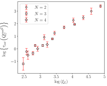
Figure 1: Behavior of the integrated auto-correlation time $\tau_{int}$ of ${Q_{U}^{cool}}^{2}$, expressed in units of the Monte Carlo updating step defined in the text, as a function of $\xi_{L}$ and $N$ for $\xi_{L}>10$. The integrated auto-correlation time was computed through a standard binned bootstrap analysis on samples obtained after $n_{cool}=50$ cooling steps.

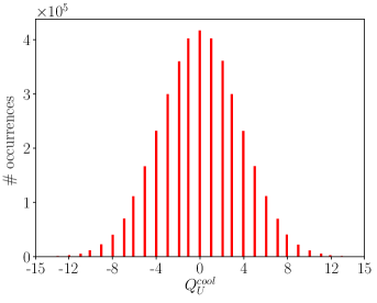
Figure 2: Distribution of the lattice topological charge $Q_{U}^{cool}$ during a run with $N=2$, $\beta=1.65$ and $L=1024$ and measured after $n_{cool}=50$ cooling steps.

Concerning the choice of the lattice size, we performed simulations at fixed $L/\xi_{L}$, ensuring that $L/\xi_{L}\sim 12$-$15$ for each run to have finite size effects under control Rossi and Vicari (1993), see Fig. 3. In those cases when that was not possible (more precisely, for high-$\xi_{L}$ runs for $N=2$), several lattices with different sizes were simulated and then the infinite volume limit was performed by fitting the $L$-dependence of every observable $\mathcal{O}$ to the law

$$\mathcal{O}(L)=\mathcal{O}_{\infty}\left(1-a\,e^{-bL/\xi_{L}}\right),$$ (21)

where $\mathcal{O}_{\infty}$ is the desired quantity and $a$ and $b$ are additional fit parameters. An example of extrapolation towards the thermodynamic limit is shown in Fig. 4.

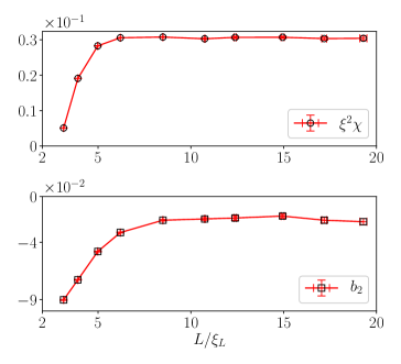
Figure 3: Example of finite size scaling of $\xi^{2}\chi$ and $b_{2}$ as a function of $L/\xi_{L}$ for $N=6$ and $\beta_{L}=0.80$ with measures taken after $n_{cool}=50$ cooling steps.

Figure 4: Examples of extrapolation towards the infinite volume limit of $\xi^{2}\chi$, $b_{2}$ and $\xi_{L}$ for $N=2$ and $\beta_{L}=1.65$ with measures taken after $n_{cool}=50$ cooling steps. Best fits of Eq. (21) performed with 4 degrees of freedom (dof) yield, respectively, $\chi^{2}/\mathrm{dof}=1.4,0.99,0.6$.

$\beta_{L}$	$L$	$\xi_{L}$	$L/\xi_{L}$	Stat. (M)
0.80	22	1.704(13)	12.9	3.2
0.85	26	2.037(16)	12.8	3.2
0.90	30	2.4764(72)	12.1	20.8
0.95	36	3.0309(28)	12.0	201
1.00	46	3.7726(48)	12.3	130
1.05	58	4.7345(59)	12.3	150
1.10	74	6.0142(91)	12.2	114
1.15	94	7.735(16)	12.3	66.7
1.20	122	9.958(51)	12.4	12.2
1.25	160	13.10(14)	12.2	3.4
1.30	210	17.16(19)	12.2	3.9
1.35	280	22.77(34)	12.3	3.6
1.40	98	29.031(40)	3.4	3.5
	198	31.115(55)	6.4	13.5
	298	31.32(19)	9.5	6.0
	396	31.41(50)	12.6	3.4
1.45	122	38.167(55)	3.2	3.5
	240	41.352(89)	5.8	8.7
	360	41.48(28)	8.7	4.0
	480	42.30(76)	11.3	2.2
1.50	168	51.43(11)	3.3	1.5
	336	55.75(21)	6.0	4.5
	504	57.26(78)	8.8	1.9
	672	56.4(1.5)	11.9	2.0
1.55	214	67.95(21)	3.1	1.5
	400	74.97(31)	5.3	3.8
	500	74.60(57)	6.7	2.4
	600	78.0(1.0)	7.7	1.6
	700	76.9(1.7)	9.1	1.2
1.60	260	88.13(34)	3.0	1.1
	400	97.92(33)	4.1	3.8
	500	98.95(59)	5.1	2.4
	600	102.23(94)	5.9	1.6
	700	98.6(1.5)	7.1	1.2
1.65	200	89.44(16)	2.2	2.4
	306	112.57(63)	2.7	0.77
	400	123.54(60)	3.2	1.5
	500	129.82(52)	3.9	3.7
	600	131.98(80)	4.5	2.5
	700	132.1(1.2)	5.3	1.8
	1024	131.4(1.5)	7.8	6.3

Table 1: Simulations summary for $N=2$. Statistics is expressed in millions (M) and every measure is taken after 10 elementary Monte Carlo steps (see the text for further details).

$\beta_{L}$	$L$	$\xi_{L}$	$L/\xi_{L}$	Stat. (M)
0.70	18	1.4797(59)	12.2	3.5
0.75	22	1.8227(76)	12.1	3.5
0.80	28	2.298(10)	12.2	3.5
0.85	36	2.906(14)	12.4	3.5
0.90	46	3.750(31)	12.3	1.5
0.95	58	4.930(23)	11.8	3.5
0.975	68	5.710(29)	11.9	3.2
1.00	80	6.588(25)	12.1	7.8
1.025	92	7.589(28)	12.1	8.3
1.05	106	8.828(32)	12.1	8.3
1.075	122	10.231(37)	11.9	8.8
1.10	146	11.834(39)	12.3	13.5
1.15	200	16.019(55)	12.5	15.5
1.20	264	21.717(71)	12.2	19.4
1.25	374	29.342(82)	12.7	37.8
1.366	720	58.69(19)	12.3	44.9

Table 2: Simulations summary for $N=3$.

$\beta_{L}$	$L$	$\xi_{L}$	$L/\xi_{L}$	Stat. (M)
0.70	22	1.7842(59)	12.3	2.8
0.75	30	2.3137(97)	13.0	2.8
0.80	38	3.039(12)	12.5	3.1
0.85	50	4.009(17)	12.5	3.1
0.90	66	5.398(22)	12.2	3.1
0.95	90	7.314(33)	12.3	3.1
1.00	120	9.997(45)	12.0	3.1
1.05	170	13.700(71)	12.4	3.1
1.10	226	18.55(10)	12.2	3.5
1.15	320	25.00(20)	12.8	3.5

Table 3: Simulations summary for $N=4$.

$\beta_{L}$	$L$	$\xi_{L}$	$L/\xi_{L}$	Stat. (M)
0.70	32	2.1263(98)	15.0	3.5
0.75	44	2.830(13)	15.5	4.6
0.80	58	3.882(20)	14.9	3.5
0.85	84	5.270(35)	15.9	3.5
0.90	106	7.149(41)	14.8	3.5
0.95	146	9.849(59)	14.8	3.5
1.00	198	13.40(11)	14.8	2.2
1.05	278	18.117(93)	15.3	7.4
1.10	368	24.77(19)	14.9	3.6

Table 4: Simulations summary for $N=5$.

$\beta_{L}$	$L$	$\xi_{L}$	$L/\xi_{L}$	Stat. (M)
0.60	18	1.4035(36)	12.8	2.6
0.65	24	1.8608(53)	12.9	2.6
0.70	32	2.5032(76)	12.8	2.5
0.75	42	3.394(11)	12.4	2.2
0.80	58	4.671(15)	12.4	2.4
0.85	78	6.389(21)	12.2	2.6
0.90	108	8.760(31)	12.3	2.6
0.95	150	11.955(48)	12.5	2.8
1.00	200	16.112(41)	12.4	6.5

Table 5: Simulations summary for $N=6$.

$\beta_{L}$	$L$	$\xi_{L}$	$L/\xi_{L}$	Stat. (M)
0.70	44	2.876(12)	15.3	2.2
0.75	58	3.940(19)	14.7	1.7
0.80	80	5.403(26)	14.8	2.4
0.85	112	7.436(35)	15.1	3.1
0.90	154	10.096(48)	15.3	3.4
0.95	210	13.717(68)	15.3	3.6
1.00	304	18.76(11)	16.2	3.9

Table 6: Simulations summary for $N=7$.

$\beta_{L}$	$L$	$\xi_{L}$	$L/\xi_{L}$	Stat. (M)
0.65	36	2.3175(76)	15.5	3.0
0.70	48	3.232(12)	14.8	2.2
0.75	68	4.452(17)	15.3	3.0
0.80	92	6.056(27)	15.2	2.4
0.85	124	8.242(42)	15.0	2.1
0.90	170	11.306(52)	15.0	2.7
0.95	240	15.164(73)	15.8	3.4

Table 7: Simulations summary for $N=8$.

3.1 Results for $\xi^{2}\chi$, $N>3$

First, we consider the case $N>3$, for which a finite continuum limit is surely expected for the topological susceptibility, with no qualitative differences in the continuum scaling compared to the large-$N$ case. For this reason, in order to extrapolate the quantity $\xi^{2}\chi$ towards the continuum limit we have fitted its dependence on $\xi_{L}$ according to the ansatz

$$f(x)=a_{0}+a_{1}x^{2}+a_{2}x^{4},\quad x=1/\xi_{L}.$$ (22)

Only for $N=4$, due to its proximity to $N=2$ and $3$ (see later discussion), we have also considered the possible presence of further power law corrections. An example of continuum extrapolation is depicted, for $N=4$, in Fig. 5.

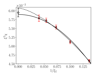
Figure 5: Extrapolation towards the continuum limit of $\xi^{2}\chi$ for $N=4$ using data in the range $\xi_{L}>6$ taken after $n_{cool}=50$ cooling steps. The solid line represents the best fit obtained using fit function $f(x)=a_{0}+a_{1}x^{2}$ (where $x=1/\xi_{L}$) while the dashed line represents the one obtained with $f(x)=a_{0}+a_{3}x^{c}$. In the latter case the exponent is $c=1.52(37)$ and best fits yield, respectively, $\chi^{2}/\mathrm{dof}=2.97/3$ and $\chi^{2}/\mathrm{dof}=1.34/2$. The diamond point represents our final estimation, see the text for more details on the assessment of systematic errors.

Several sources of systematic errors have been checked: first, the extrapolation was performed fitting data in several ranges of $\xi_{L}$ to check that the obtained extrapolations were all consistent with each other and that, as the fit range is restricted, the $O(x^{4})$ corrections became negligible. Second, as anticipated in Sec. 2.4, we extrapolated the continuum limit at fixed number of cooling step $n_{cool}$ for several values of $n_{cool}$, checking that this procedure does not introduce significant systematics in continuum-extrapolated values.

When changing the number of cooling steps, we observe that, while measures at coarse lattice spacing differ, the dependence on $n_{cool}$ is less and less visible as the continuum limit is approached, making the continuum extrapolation stable as $n_{cool}$ is varied. In Fig. 6 we show an example of the continuum extrapolation at two different values of $n_{cool}$ for $N=5$ while, in Fig. 7, we show, for the same case, that any variation in the continuum extrapolation observed when changing $n_{cool}$ is well contained inside our statistical errors.

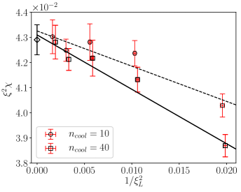
Figure 6: Extrapolation towards the continuum limit of $\xi^{2}\chi$ for $N=5$ using data in the range $\xi_{L}>7$. The solid line represents the best fit obtained using fit function $f(x)=a_{0}+a_{1}x^{2}$ (where $x=1/\xi_{L}$) with measures taken after $n_{cool}=40$ cooling steps while the dashed line represents the one obtained with the same fit function with $n_{cool}=10$ cooling steps. The best fits yield, respectively, $\chi^{2}/\mathrm{dof}=1.68/3$ and $\chi^{2}/\mathrm{dof}=2.25/3$. Data obtained for different numbers of cooling steps have been plotted slightly shifted to improve readability. The diamond point represents our final estimation of the continuum limit.

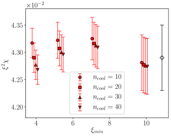
Figure 7: Example of study of systematic errors on the continuum extrapolation of $\xi^{2}\chi$ for $N=5$ and for 4 different number of cooling steps $n_{cool}$. Extrapolations obtained for different values of $n_{cool}$ are plotted slightly shifted to improve readability. This extrapolations are all obtained using the fit function $f(x)=a_{0}+a_{1}x^{2}$, where $x=1/\xi_{L}$. The diamond point represents our final estimation of the continuum limit.

The final, continuum determinations obtained for $\xi^{2}\chi$ are reported in Tab. 8.

Some of our results can be compared with previous literature. For instance, the case $N=4$ was studied also in Ref. Campostrini et al. (1992b), reporting a continuum extrapolation $\xi^{2}\chi(N=4)=0.06$ with an error of the order of 10 %, which is in agreement with our present result $\xi^{2}\chi(N=4)=0.0595(12)$, even if with a larger uncertainty. For $N=6$ one can find a previous determination in Ref. Lian and Thacker (2007): even if no continuum extrapolation is reported there, the result at the smallest explored lattice spacing, $\xi^{2}\chi(N=6)\simeq 0.037(6)$, is consistent with our continuum extrapolation, $\xi^{2}\chi(N=6)=0.0338(3)$. In both cases, the increased accuracy of our determinations is mostly due to the larger statistics and/or number of simulation points adopted for the continuum extrapolation.

3.2 Results for $\xi^{2}\chi$, $N=3$

In the $N=3$ case we fit the dependence of $\xi^{2}\chi$ on $\xi_{L}$ according to the following function:

$$g(x)=a_{0}+a_{1}x^{2}+a_{2}x^{4}+a_{3}x^{c},\quad x=1/\xi_{L},$$ (23)

where we consider both the extrapolations obtained with fixed $c=1$, as suggested by the ansatz in Eq. (20), and with $c$ left as a free parameter. In both cases, the ansatz in Eq. (23) provides a very good description of our numerical results, and the $x^{4}$ corrections turn out to be necessary only when considering in the fit range correlation lengths as small as $\xi_{L}\lesssim 5$. Moreover, even when $c$ is treated as a free parameter, its values turn out to be compatible with 1 within errors, thus giving further numerical support to the ansatz in Eq. (20).

Examples of continuum extrapolations are shown in Fig. 8, where we also report our final continuum estimate for $N=3$, $\xi^{2}\chi=0.110(5)$. The quoted error includes all possible systematics related to the variability of the fit parameter $a$ when changing the fitting ansatz, the fitting range (with $\xi_{min}$ varied between 2 and 7) and the number of cooling steps (with $n_{cool}$ varied between 10 and 50).

Also in this case, a comparison with previous literature is appropriate and interesting. Early results obtained in Ref. Petcher and Lüscher (1983), $\xi^{2}\chi(N=3)\simeq 0.09$, were not far from our present estimate, even if no error was quoted in that case. However, later results pointed out to a possible wrong scaling of $\chi$ towards the continuum limit, hence to a possible divergence of $\chi$ even for $N=3$ Lian and Thacker (2007). Our present results show that $\xi^{2}\chi$ is in fact finite for $N=3$, even if the continuum limit extrapolation needs special care, because of the small instanton contributions. Since this point was debated in previous literature, it is important to stress that our continuum extrapolation for $N=3$ is fully confirmed by the small-$N$ extrapolation based on $N>3$ results that we present in section 3.4.

Let us now discuss more in detail the systematics related to cooling. Fig. 8 shows that results obtained for $n_{cool}=10$ and $50$ are significantly different from each other, nevertheless, as also evident for one particular fit ansatz in Fig. 8, their continuum limit shows very little variations, when compared to statistical errors on the fit parameters. There is a simple way to understand why results at different $n_{cool}$ differ so much at finite $\xi_{L}$, while coinciding in the $\xi_{L}\to\infty$ limit. As already discussed in Sec. 2.4, cooling acts as a diffusive process which smooths away field fluctuations (both physical and unphysical) below an effective radius $r=a\hat{r}(n_{cool})$, where the radius in lattice spacing units, $\hat{r}$, is a function of $n_{cool}$ only, i.e. independent of the lattice spacing $a$. At fixed lattice spacing, different values of $n_{cool}$ lead to different values of $r$ hence to different values of the topological susceptibility, because a different amount of physical signal below $r$ is removed: the effect can be particularly significant for small $N$, where topological fluctuations at small scales are more abundant. On the other hand, the effect must fade away as $a\to 0$.

If the above picture is correct, results obtained at different $a$ and different $n_{cool}$, but such that $r=a\hat{r}(n_{cool})$ is the same, should coincide: for instance, results shown in Fig. 8 for $n_{cool}=10$ should go onto those at $n_{cool}=50$ if they are shifted along the horizontal axis by a constant factor equal to $\hat{r}(10)/\hat{r}(50)$. Such experiment has been performed for $n_{cool}=10,25,50$ in Fig. 9, showing that it works perfectly: plotting all data as a function of an effective variable $x_{\rm eff}$ proportional to $r/\xi=\hat{r}(n_{cool})/\xi_{L}$, where $\hat{r}(n_{cool})$ has been found empirically, data at different values of $n_{cool}$ collapse perfectly onto each other over the whole range of explored correlation lengths; a similar collapse can be obtained also for other values of $N$. Therefore, the dependence of $\xi^{2}\chi$ on $n_{cool}$ observed at finite lattice spacing can indeed be simply interpreted in terms of a global effective rescaling of $1/\xi_{L}$, so that such dependence naturally fades away when $\xi_{L}\to\infty$.

To summarize, our results for $N=3$ provide solid evidence that $\xi^{2}\chi$ is indeed finite in the continuum limit of this theory. On the other hand, that will be further checked and supported by an independent small-$N$ extrapolation based on $N>3$ results only, which is discussed in Sec. 3.4 and will make the evidence conclusive.

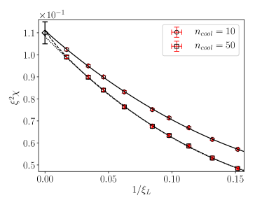
Figure 8: Extrapolation towards the continuum limit of $\xi^{2}\chi$ for $N=3$ using data in the range $\xi_{L}>6$. The dashed and dotted lines represent, respectively, the best fits obtained for $n_{cool}=50$ using fit function $g(x)=a_{0}+a_{1}x^{2}+a_{3}x^{c}$ (where $x=1/\xi_{L}$) either leaving $c$ as a free parameter ($\chi^{2}/\mathrm{dof}=2.4/6$) or with fixed $c=1$ ($\chi^{2}/\mathrm{dof}=1.3/5$); in the latter case the free exponent turns $c=0.85(14)$. The solid line, instead, represents the best fit obtained with $c$ as a free parameter for $n_{cool}=10$ cooling steps: in this case $c=0.98(18)$ ($\chi^{2}/\mathrm{dof}=1.35/5$). The diamond point represents our final estimation of the continuum limit, which takes into account all systematics related to the variability in fitting function, fitting range and number of cooling steps.

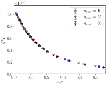
Figure 9: Results obtained for $\xi^{2}\chi$ in the $N=3$ model and for different number of cooling steps, plotted as a function of an effective variable $x_{\rm eff}$ proportional to $\hat{r}(n_{cool})/\xi_{L}=r/\xi$. The perfect collapse of data proves that the dependence of $\xi^{2}\chi$ on $n_{cool}$ can be interpreted in terms of varying effective radius $r=a\hat{r}(n_{cool})$ below which the topological signal is lost, and as such disappears after continuum extrapolation $a\to 0$. The exact value of $x_{\rm eff}$ has been fixed conventionally to $x_{\rm eff}=(\hat{r}(n_{cool})/\xi_{L})/\hat{r}(n_{cool}=50)$ and we have found empirically $\hat{r}(25)/\hat{r}(50)\simeq 1.1$ and $\hat{r}(10)/\hat{r}(50)\simeq 1.3$.

3.3 Results for $\xi^{2}\chi$, $N=2$

For the $N=2$ case two possibilities are open. The ansatz based on Eq. (20) could be correct, leading to a susceptibility which diverges logarithmically in the continuum limit, i.e. has the following dependence on $x=1/\xi_{L}$:

$$\xi^{2}\chi(\xi_{L})=a_{0}^{\prime}\log(x/a_{1}^{\prime})+a_{2}^{\prime}x^{2}+a_{3}^{\prime}x^{4}.$$ (24)

On the other hand, corrections to such prediction leading to a finite $\xi^{2}\chi$ cannot be excluded a priori, in this case one should consider a dependence on $\xi_{L}$ like that used in Eq. (23) for the $N=3$ case, i.e.:

$$\xi^{2}\chi(\xi_{L})=a_{0}+a_{1}x^{2}+a_{2}x^{4}+a_{3}x^{c}.$$ (25)

where $c$ is a positive exponent. We have to say that, unfortunately, despite the fact that our present results extend over almost two orders of magnitudes in terms of the correlation length $\xi_{L}$, we are still not able to clearly distinguish between the two possibilities, in the sense that both ansätze, Eqs. (24) and (25), return acceptable values of the $\chi^{2}/\mathrm{dof}$ test, even if marginally better for the convergent ansatz.

Let us consider, for instance, the data reported in Fig. 10, where we consider only results obtained for $\xi_{L}>10$. In this range $O(x^{4})$ corrections turn out to be unnecessary. Considering data obtained for $n_{cool}=50$ we obtain $\chi^{2}/\mathrm{dof}=7.9/6$ for the divergent ansatz in Eq. (24) and $\chi^{2}/\mathrm{dof}=3.8/5$ for the convergent ansatz in Eq. (25); in the latter case we also obtain $c=0.30(15)$ and a prediction $\xi^{2}\chi=0.43(12)$ (for $n_{cool}=20$, the latter prediction changes to $\xi^{2}\chi=0.42(11)$, $c=0.33(16)$, with $\chi^{2}/\mathrm{dof}=3.8/5$). Notice that, in the case of the convergent fit, the coefficient $c$ is at two standard deviations from zero, which is the boundary where also this fit becomes divergent: this is consistent with the fact that the logarithmic fit is marginally acceptable.

The situation does not change appreciably when changing the fit range, with both ansätze remaining acceptable even if with slightly lower values of the $\chi^{2}/\mathrm{dof}$ test in the case of a finite continuum susceptibility: if the latter scenario could be assumed a priori we would conclude $\xi^{2}\chi\sim 0.40(15)$ for $N=2$. However, the fact that no conclusive answer can be obtained based on our present data for $N=2$, is confirmed by looking at the best fit curves reported in Fig. 10: the two curve profiles (convergent and divergent) are hardly distinguishable in the explored range of $\xi_{L}$ and deviate from each other only for much larger values of $\xi_{L}$.

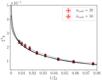
Figure 10: Extrapolation towards the continuum limit of $\xi^{2}\chi$ for $N=2$ using data in the range $\xi_{L}>10$. The solid and dashed lines represent, respectively, the best fits obtained using fit functions $h(x)=a_{0}^{\prime}\log(x/a_{1}^{\prime})+a_{2}^{\prime}x^{2}$ (where $x=1/\xi_{L}$) and $g(x)=a_{0}+a_{1}x^{2}+a_{2}x^{4}+a_{3}x^{c}$ with measure taken after $n_{cool}=50$ cooling steps. The former best fit yields $\chi^{2}/\mathrm{dof}=7.9/6$ while, in the latter case, we obtain the continuum limit $a=0.43(12)$ and the exponent $c=0.30(15)$ ($\chi^{2}/\mathrm{dof}=3.8/5$). The dotted line, instead, represents again the best fit obtained using fit function $g(x)=a_{0}+a_{1}x^{2}+a_{2}x^{4}+a_{3}x^{c}$ but with measures taken after $n_{cool}=20$, which gives $a=0.42(11)$ and $c=0.33(16)$ ($\chi^{2}/\mathrm{dof}=3.8/5$).

Another independent possibility to discriminate between these two different behaviors is to use data obtained for $N>2$ and extrapolate them towards $N=2$. This topic is covered in Sec. 3.4.

3.4 $N\to 2$ limit of $\xi^{2}\chi$

In this section we aim at tackling the question about the small $N$ behavior of the topological susceptibility from another independent front, by extrapolating continuum results obtained for $\xi^{2}\chi$ at $N>2$ towards $N=2$. A summary of such results, including all $N<10$, is reported in Tab. 8.

$N$	$\xi^{2}\chi\cdot 10^{3}$
3	110(5)
4	59.5(1.2)
5	42.90(60)
6	33.80(30)
7	27.10(30)
8	22.40(30)
9*	20.00(15)

Table 8: Summary of continuum extrapolations of $\xi^{2}\chi$ as a function of $N$. The value marked with * is taken from Ref. Bonanno et al. (2019).

Using Eq. (7) and assuming non-interacting instantons, the expected behavior of $\xi^{2}\chi$ when approaching the $N\to 2$ limit is Bonanno et al. (2019)

$$\xi^{2}\chi\sim\frac{1}{N-2},\quad N>2.$$ (26)

Therefore, we fitted the $N$-dependence of $\xi^{2}\chi$ for $N>2$ using the following function:

$$F(N)=\frac{a}{(N-N^{*})^{\gamma}}.$$ (27)

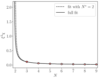
Figure 11: Best fit of the small-$N$ behavior of $\xi^{2}\chi$ for $N$ ranging from 3 to 9. The solid and dashed lines represent, respectively, the best fits obtained using fit function (27) with $N^{*}=2$ or left as a free parameter. The best fits yield, respectively, $\chi^{2}/\mathrm{dof}=5.1/5$ and $\chi^{2}/\mathrm{dof}=4.56/4$.

The best fit is quite good and is shown in Fig. 11, the corresponding parameters are the following:

$$a = 0.119(10),$$

$$N^{*} = 1.90(14),$$

$$\gamma = 0.91(4),$$

$$\chi^{2}/\mathrm{dof} = 4.56/4.$$

This best fit, yielding a central value for $N^{*}<2$, technically supports a finite extrapolation towards $N=2$; however, $N=2$ is well within one standard deviation from $N^{*}$, so that even this approach reveals to be inconclusive, at least for this issue. As shown in Fig. 12, the error on the best fit blows up as $N\to 2$ is approached, being $N^{*}$ very close to it, so that this extrapolation turns out to be compatible with the hypothetical finite value found from the convergent continuum limit of Sec. 3.3, $\xi^{2}\chi=0.40(15)$, but within quite large uncertainties. As a matter of fact, a best fit of the same data set with (26) but fixing $N^{*}=2$ yields a perfectly compatible results: $a=0.112(2)$ and $\gamma=0.89(1)$ ($\chi^{2}/\mathrm{dof}=5.1/5$); this best fit is depicted in Fig. 11 as well.

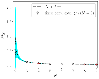
Figure 12: Best fit of the small-$N$ behavior of $\xi^{2}\chi$ for $N$ ranging from 3 to 9. The dashed line represents the best fit obtained using fit function (27) leaving $N^{*}$ as a free parameter, the shadowed band represents the fit error and the diamond points represent the hypothetical finite continuum limit obtained from the convergent continuum extrapolation of $\xi^{2}\chi$ for $N=2$.

Finally, as a further consistency check of the solidity of these results, we fitted our small-$N$ data also in narrower ranges, in particular considering only data for $N>3$ or for $N>4$. Best fits are shown in Fig. 13. In both cases, $N^{*}$ and $\gamma$ turned out, again, to be compatible with 2 and 1 respectively:

$$N^{*} =1.77(31),\, \gamma =0.94(7),\quad N>3,$$

$$N^{*} =2.40(52),\, \gamma =0.82(10),\quad N>4.$$

Moreover, extrapolating these fits towards $N=3$, we obtain values for $\xi^{2}\chi(N=3)$ which are, in both cases, in perfect agreement with the continuum limit obtained from direct $N=3$ simulations in Sec. 3.2. Based on these results, we conclude that the finiteness of the topological susceptibility for $N=3$ can be definitely assessed.

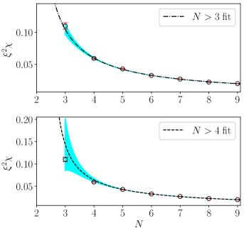
Figure 13: Best fits of the small-$N$ behavior of $\xi^{2}\chi$ considering just $N>3$ or $N>4$ data. The dashed lines represent the best fits obtained using fit function (27) leaving $N^{*}$ as a free parameter, while the shadowed bands represent the fit errors. Best fits give, respectively, $N^{*}=1.77(31)$ ($\chi^{2}/\mathrm{dof}=4.3/3$) and $N^{*}=2.40(52)$ ($\chi^{2}/\mathrm{dof}=3/2$). Such extrapolations fully support the finite results obtained from direct simulations at $N=3$, both qualitatively and quantitatively.

3.5 Small-$N$ behavior of the $b_{2n}$ coefficients

In this section we study the small-$N$ behavior of the $b_{2n}$ coefficients, in particular, we aim at checking the hypothesis that these coefficients are finite in the $N\to 2$ limit and that, in this limit, they approach the DIGA prediction. With our statistics, we could only obtain reliable estimations of $b_{2}$, while already $b_{4}$ always turned out to be compatible with zero, after continuum extrapolation, in all explored cases. Thus, we can presently discuss only the small-$N$ behavior of $b_{2}$.

As we have discussed in Sec. 2.3, contrary to what happens for the topological susceptibility, in this case we do not expect a priori modifications to the standard form of UV corrections reported in Eq. (17). As a confirmation of this expectation, a continuum extrapolation performed according to the fit function in Eq. (22) turns out to work well for all values of $N$, including $N=2$ and $N=3$, with $O(x^{4})$ corrections becoming irrelevant and not needed when restricting the fit range to large enough correlation lengths. Examples of such extrapolations are reported in Figs. 14, 15 and 16.

For $N=2$ and $3$ we have also considered the possible addition of generic power law corrections to Eq. (22) proportional to $x^{c}$, as we have done for $\xi^{2}\chi$, however this turned out to be irrelevant in this case, with modifications to the continuum extrapolation staying within errors. The only modification which can be noticed in the $N=2,3$ cases is that the approach to the continuum limit is steeper, however this is compensated by the larger values of $\xi_{L}$ available from our simulations in these cases.

All continuum extrapolations are reported in Tab. 9. Also in this case the quoted errors include systematics, which have been assessed by observing the variation of central fit values when changing the fit function, the fit range and the number of cooling steps $n_{cool}$.

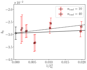
Figure 14: Extrapolation towards the continuum limit of $b_{2}$ for $N=5$ using data in the range $\xi_{L}>7$. The solid and dashed lines represent the best fits obtained using fit function $f(x)=a_{0}+a_{1}x^{2}$ (where $x=1/\xi_{L}$) with measures taken, respectively, after $n_{cool}=10$ and $n_{cool}=40$ cooling steps. Best fits yield, respectively, $\chi^{2}/\mathrm{dof}=2.25/3$ and $\chi^{2}/\mathrm{dof}=3.24/3$. Data obtained for different numbers of cooling steps have been plotted slightly shifted to improve readability. The diamond point represents our final estimation of the continuum limit.

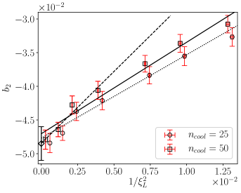
Figure 15: Extrapolation towards the continuum limit of $b_{2}$ for $N=3$. The solid and dashed lines represent the best fits obtained using the fit function $g(x)=a_{0}+a_{1}x^{2}$ (where $x=1/\xi_{L}$) using measures taken after $n_{cool}=50$ cooling steps in the ranges $\xi_{L}>8$ and $\xi_{L}>15$. The best fits yield, respectively, $a_{0}=-0.0471(8)$ ($\chi^{2}/\mathrm{dof}=4.65/5$) and $a_{0}=-0.0485(11)$ ($\chi^{2}/\mathrm{dof}=1.06/2$). The dotted line represents instead the best fit obtained using measures taken after $n_{cool}=20$ cooling steps in the range $\xi_{L}>8$. The best fit yields $a_{0}=-0.0478(8)$ with $\chi^{2}/\mathrm{dof}=2.85/5$. Data obtained for different numbers of cooling steps have been plotted slightly shifted to improve readability. The diamond point represents our final estimation of the continuum limit.

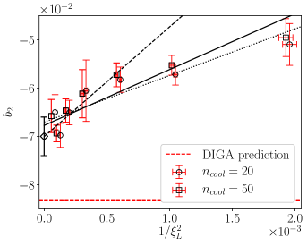
Figure 16: Extrapolation towards the continuum limit of $b_{2}$ for $N=2$. The solid and dashed lines represent the best fits obtained using the fit function $g(x)=a_{0}+a_{1}x^{2}$ (where $x=1/\xi_{L}$) using measures taken after $n_{cool}=50$ cooling steps in the ranges $\xi_{L}>20$ and $\xi_{L}>30$. The best fits yield, respectively, $a_{0}=-0.0677(13)$ ($\chi^{2}/\mathrm{dof}=6.95/5$) and $a_{0}=-0.0700(17)$ ($\chi^{2}/\mathrm{dof}=2.13/3$). The dotted line represents instead the best fit obtained using measures taken after $n_{cool}=20$ cooling steps in the range $\xi_{L}>20$. The best fit yields $a_{0}=-0.0670(16)$ with $\chi^{2}/\mathrm{dof}=4.55/5$. Data obtained for different numbers of cooling steps have been plotted slightly shifted to improve readability. The diamond point represents our final estimation of the continuum limit.

$N$	$b_{2}\cdot 10^{3}$
2	-70.0(4.0)
3	-48.5(2.5)
4	-38.5(2.5)
5	-29.5(2.5)
6	-28.0(2.0)
7	-20.5(3.5)
8	-19.0(3.0)
9*	-13.90(13)

Table 9: Summary of continuum extrapolations of $b_{2}$ as a function of $N$. The value marked with * is taken from Ref. Bonanno et al. (2019).

Our data for $N=2$ confirm that $b_{2}$ is finite, with a continuum estimate $b_{2}(N=2)=-0.070(4)$ which is $\sim 3\sigma$ off from the DIGA prediction $b_{2}^{\mathit{DIGA}}=-1/12\simeq-0.0833$. Results reported in Ref. Bietenholz et al. (2016) point also to $b_{2}\sim-1/12$, even if no continuum limit is performed in that case.
We can try to extrapolate, based on present results, the value $N^{*}$ of $N$ for which $b_{2}$ reaches the DIGA prediction, to that aim we try to fit our data according to a critical behavior like:

$$G(N)=b_{2}^{\mathit{DIGA}}+a(N-N^{*})^{\gamma}.$$ (28)

While we do not have any argument to support such an ansatz, it turns out to work quite well: a best fit in the range $[2,9]$ is reported in Fig. 17 and returns the following parameters:

$$a = 0.0345(18),$$

$$N^{*} = 1.94(6),$$

$$\gamma = 0.352(25),$$

$$\chi^{2}/{\rm dof} = 1.2/5.$$

It is interesting to observe that the $N^{*}$ found in this way from the analysis of $b_{2}$ is perfectly compatible with the one found for the critical fit of $\xi^{2}\chi$, and still compatible with $N^{*}=2$.

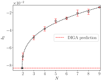
Figure 17: Small-$N$ behavior of the quartic coefficient $b_{2}$. The solid lines represent the best fit obtained using fit function (28). The best fit yields $N^{*}=1.94(6)$ with $\chi^{2}/\mathrm{dof}=1.2/5$. The black point represents the found interval for $N^{*}$, for which $b_{2}(N^{*})=b_{2}^{\mathit{DIGA}}$.

4 Conclusions

In this work, we have presented a systematic numerical study of the peculiar features of the $\theta$-dependence around $\theta=0$ of the vacuum energy $f(\theta)$ of $2d$ $CP^{N-1}$ models in the small-$N$ limit. To that aim, we have performed numerical simulations for $N\in[2,8]$.

One of the most interesting questions regards the value of $N$, if any, at which the topological susceptibility $\chi$ diverges: this is predicted to be $N=2$ by perturbative computations of the instanton size distribution. A second interesting question regards the fate of the $b_{2n}$ coefficients, which parametrize the non-quadratic part of $\theta$-dependence and which could possibly approach the values predicted by the Dilute Instanton Gas Approximation at the point where $\chi$ diverges, if the theory can be approximated in this case by a gas of small and non-interacting instantons and anti-instantons.

Our strategy has been twofold. On one hand, we have dedicated particular efforts to correctly assess the continuum limit of $\xi^{2}\chi$ for $N=2$ and $N=3$ from direct simulations of these theories: to that aim, we have performed simulations on lattices with correlations lengths ranging from a few units up to $O(10^{2})$. On the other hand, we have exploited results obtained for larger values of $N$, where the continuum extrapolation is easier, in order to perform a small-$N$ extrapolation. Based on this double strategy, we have obtained consistent and conclusive evidence that the topological susceptibility is finite for $N=3$, providing the estimate $\xi^{2}\chi=0.110(5)$. We would like to stress that, since the convergence of $\xi^{2}\chi$ in the continuum limit for $N=3$ was debated in previous literature, a double check with two different and independent methods is important for our final assessment about this issue.

On the other hand, results for $N=2$ are still inconclusive: results obtained directly at $N=2$ are consistent with a logarithmically-divergent continuum extrapolation, but do not yet exclude a finite continuum value with $\xi^{2}\chi\sim 0.4$, which is even marginally favored from the point of the $\chi^{2}/\mathrm{dof}$ test. A similar picture emerges from the extrapolation from results obtained for $N>2$, which provides evidence for a critical behavior $\xi^{2}\chi\propto 1/(N-N^{*})^{\gamma}$, with $N^{*}=1.90(14)$. Therefore, future numerical studies are still needed in this case to definitely settle the issue.

As for the $b_{2}$ coefficient, we have provided continuum extrapolations down to $N=2$. While there is no compelling reason to expect that the DIGA prediction be valid at the point where $\xi^{2}\chi$ diverges, it is interesting to observe that our numerical results are consistent with that. For $N=2$ we obtain $b_{2}(N=2)=-0.070(4)$, i.e., around $3\sigma$ off the DIGA value $b_{2}^{\mathit{DIGA}}=-1/12\simeq-0.0833$, while an extrapolation from our results at all values of $N$ (see Eq. (28)) provides evidence for $b_{2}$ reaching $b_{2}^{\mathit{DIGA}}$ for $N=1.94(6)$, which is consistent with the value $N^{*}$ at which $\xi^{2}\chi$ diverges reported above.