Modelling Mullins Effect Induced by Chain Delamination and Reattachment

Abstract

We propose a continuum theory to model the Mullins effect, which is ubiquitously observed in polymer composites. In the theory, the softening of the materials during the stretching process is accounted for by considering the delamination of polymer chains from nano-/micro-sized fillers, and the recovery effect during the de-stretching process is due to the reattachment of the polymer chains to nano-/micro-sized fillers. By incorporating the chain entanglements, Log-Normal distribution of the mesh size in the network, etc., we can obtain a good agreement between our numerical calculation results and existing experimental data. This physical theory can be easily adapted to meet more practical needs and utilised in analysing mechanic properties of polymer composites.

I Introduction

Polymer composites  Vilgis et al. (2009); Saheb and Jog (1999); Ku et al. (2011); Sanjay et al. (2018); Donnet (2003); Mohammed et al. (2015); Sanjay et al. (2016) are mixtures of polymer chains with reinforcing filler particles (also named as ‘filled rubber elastomer’), and can be further categorised into micro or nano-composites depending on the size of the fillers. By adding fillers into the polymer network, one can easily adjust material properties such as elasticity, thermal conductivity  Mu et al. (2007); Ramnath et al. (2014) and wet grip  Ren and Cornish (2019); Choi et al. (2018); Kim et al. (2019), and can also make the rubber more durable against material fatigue  Mars and Fatemi (2002); Bathias (2006); Dong et al. (2014). Thus, filled rubbers have been utilised in numerous daily and industrial applications including tires, seals, medical equipments, etc Vilgis et al. (2009); Sanjay et al. (2016); Ramakrishna et al. (2001); Mohammed et al. (2015).

A pertinent phenomenon of such polymer composites is Mullins effect: when the material is first stretched and then de-stretched, the de-stretch stress-strain curve lies below the stretch curve and there is a residual strain of the material, and it is called as ‘ideal’ Mullins effect if the stress achieved during the re-stretch coincides with the first de-stretch curve. On the other hand, it is called as ‘non-ideal’ if the re-stretch curve is somewhere in between the first stretch and the first de-stretch curve, i.e., there is partial recovery up to the maximum strain ever attained, and the stress-strain response resembles a virgin material upon further stretching when exceeding the maximum strain ever reached in the deformation history Diani et al. (2009); Mullins (1948). Several mechanisms have been proposed for understanding Mullins effect, such as bond rupture Blanchard and Parkinson (1952), molecules slipping Houwink (1956), filler rupture Kraus et al. (1966) and disentanglement Hanson et al. (2005), but a consensus has yet to be reached due to the absence of direct experimental evidence.

A recent experiment has provided new insights into Mullins effect Varol et al. (2020): it was shown that under cyclic loading conditions, the polymer chain anisotropy increased together with Mullins softening, indicating that reversible chain delamination may account for the observed Mullins effect. An illustration of this proposed mechanism is shown in Figure 1. Furthermore, no significant change in aggregate size was detected, casting doubt on whether aggregate interactions were indeed important.

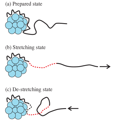
Figure 1: Illustration of delamination-induced Mullins effect. A polymer chain (black) is partly attached to a filler aggregate (blue circles) in the prepared state (a), and partial delamination occurs upon stretching (b), leading to softening. The delaminated portion is highlighted with red dotted line. When the material is de-stretched as in (c), part, but not all, of the delaminated chain reattaches back to the aggregate and the softening effect is partially recovered. The portion of reattached chain is indicated with black dotted line.

In the present work, we propose a continuum model of the energy density function to incorporate the chain delamination and the chain reattachment process, and demonstrate its merit by explaining Mullins effect within our framework. We start with the ideal Mullins effect, showing how delamination alone accounts for softening and residual stretch; then we introduce more practical details including chain reattachment, the distribution of chain length, chain entanglements, etc., from which the non-ideal Mullins effect is recovered, and a comparison of the numerical calculation to experimental data is given.

II Ideal Mullins effect

II.1 Gaussian chain case

Suppose that a polymer chain bridging two neighboring filled aggregates consists of $n$ segments, which is not a constant but instead a function of ever experienced deformation, such that $n\equiv\eta\cdot n_{0}$, with $\eta$ representing the relative elongation of the chain and $n_{0}$ as the initial segment number before any deformation. In the Gaussian limit Boyce and Arruda (2000), by denoting $\mathbf{r}$ as the chain end-to-end vector and $l$ as the segment size, the probability density of finding such a chain with given $\mathbf{r}$ is

$$P(\mathbf{r})=\left(\frac{3}{2\pi\eta n_{0}l^{2}}\right)^{\frac{3}{2}}\exp\left(-\frac{3\mathbf{r}^{2}}{2\eta n_{0}l^{2}}\right),$$ (1)

and the corresponding stretch ratio of the chain is defined as $\lambda\equiv|\mathbf{r}|/\sqrt{n_{0}}l$.

For a polymer network composed of the above Gaussian chains, which is deformed with the stretching ratios along three orthogonal directions as $\lambda_{1}$, $\lambda_{2}$ and $\lambda_{3}$, respectively, its energy density function, $F$, can be obtained by using the three-chain model Wang and Guth (1952); Meng and Terentjev (2017); Boyce and Arruda (2000); Meng and Terentjev (2016),

$$F(\lambda_{1,2,3},\eta_{1,2,3})=\frac{1}{2}Nk_{\textmd{B}}T\left(\frac{\lambda_{1}^{2}}{\eta_{1}}+\frac{\lambda_{2}^{2}}{\eta_{2}}+\frac{\lambda_{3}^{2}}{\eta_{3}}\right)+\textmd{...}$$ (2)

where $N$ is the number density of chains, $k_{\textmd{B}}$ is the Boltzmann factor and $T$ is temperature. This energy expression is also known as the neo-Hookean model. The omitted terms are independent of $\lambda_{1,2,3}$ and drop out during stress calculations.

By uniaxially stretching the material in the $i=3$ direction with the stretch ratio as $\lambda_{3}$, then there is $\lambda_{1}=\lambda_{2}=1/\sqrt{\lambda_{3}}$ by considering the incompressibility of the material, i.e., $\lambda_{1}\lambda_{2}\lambda_{3}=1$. For simplicity, we will replace $\lambda_{3}$ with $\lambda$ in the following discussions. By assuming there is no chain delamination in the $i=1,2$ directions, i.e., $\eta_{1}=\eta_{2}=1$, the tensile stress can be obtained as, after dropping the subscripts:

$$\sigma(\lambda,\eta)=\frac{\partial F}{\partial\lambda}=Nk_{\textmd{B}}T\left(\frac{\lambda}{\eta}-\frac{1}{\lambda^{2}}\right).$$ (3)

The residual strain after the de-stretching can be easily obtained by setting the above tensile stress to zero, giving

$$\varepsilon_{\textmd{residual}}=\lambda_{\textmd{residual}}-1=\sqrt[3]{\eta}-1,$$ (4)

which is positive for $\eta>1$.

For demonstrative purposes, we here introduce a toy model for $\eta$:

1. the changing rate of $\eta$ with respect to the stretch: $\mathrm{d}\eta/\mathrm{d}\lambda=k$ for $\lambda\geq\lambda_{\textmd{max}}$, where $\lambda_{\textmd{max}}$ is the maximum stretch ever attained in the past deformation history and $k$ denotes the delamination rate;

2. $\mathrm{d}\eta/\mathrm{d}\lambda=0$ for $\lambda<\lambda_{\textmd{max}}$.

The stress-stretch response is shown in Figure 2. In the Gaussian limit, the stress-stretch response of a chain with constant chain length approaches a linear trend at large stretches and the gradient drops with larger relative elongation, leading to decreasing gradients of the de-stretching curves at relaxation points (circles in Figure 2). This is in stark contrast to the almost-vertical gradients for relaxation stress-stretch curves seen in experiments Diani et al. (2009); Andriyana et al. (2015); Chagnon et al. (2004); Dargazany and Itskov (2009) and an important reason is that when a chain is close to the point of delamination, the physical end-to-end distance might be the same order as the contour length of the polymer chain; in this case, Langevin chain statistics Kuhn and Grün (1942); Boyce and Arruda (2000), rather than the Gaussian one, is needed.

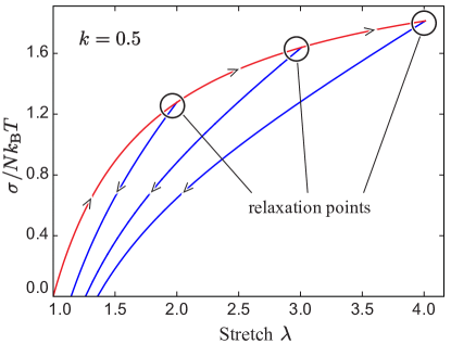
Figure 2: Stress-stretch response of the Gaussian chain system. Red and blue lines denote the stress-stretch relations during the stretching process and the de-stretching process, respectively.

II.2 Langevin chain case

In the non-Gaussian limit, we adopt the Langevin chain statistics treatment Boyce and Arruda (2000); Kuhn and Grün (1942) under the three-chain framework. The energy of a chain with the end-to-end length $r$ and the segment number $n_{0}$ is

$$W_{\textmd{L}}(r,n_{0})=\sqrt{n_{0}}k_{\textmd{B}}T\left[\frac{r}{\sqrt{n_{0}}l}\beta+\sqrt{n_{0}}\ln\left(\frac{\beta}{\sinh(\beta)}\right)\right],$$ (5)

with $\beta\equiv\mathcal{L}^{-1}(\frac{r}{n_{0}l})$ as the inverse Langevin function, which in our numerical calculation is approximated by the R. Jedynak form Jedynak (2015): $\mathcal{L}^{-1}(x)\approx x(3.0-2.6x+0.7x^{2})/[(1-x)(1+0.1x)]$ with a maximum fractional error of 1.5%. By using the earlier prescription in the Gaussian chain case and replacing $n$ and $r$ with $\eta$, $n_{0}$ and $\lambda$, we arrive at

$$W_{\textmd{L}}(\lambda,\eta,n_{0})=\sqrt{n_{0}}k_{\textmd{B}}T\left[\lambda\beta+\eta\sqrt{n_{0}}\ln\left(\frac{\beta}{\sinh(\beta)}\right)\right],$$ (6)

with $\beta=\mathcal{L}^{-1}\left(\frac{\lambda}{\eta\sqrt{n_{0}}}\right)$. Note that in the small stretch limit, equation (6) reduces to the Gaussian limit:

$$\lim\limits_{\lambda/\sqrt{n_{0}}\rightarrow 0}W_{\textmd{L}}[\lambda,\eta,n_{0}]=\frac{3}{2}k_{\textmd{B}}T\cdot\frac{\lambda^{2}}{\eta}.$$ (7)

With the three chain model, we can obtain the energy density function:

$$\begin{split}F&(\lambda_{1,2,3},\eta_{1,2,3},n_{0})=\\ &\frac{Nk_{\textmd{B}}T}{3}\sqrt{n_{0}}\sum_{i=1}^{3}\left[\lambda_{i}\beta_{i}+\eta_{i}\sqrt{n_{0}}\ln\left(\frac{\beta_{i}}{\sinh(\beta_{i})}\right)\right].\end{split}$$ (8)

Then the tensile stress of a uniaxially stretched material with the stretch ratio $\lambda$, can be obtained as:

$$\begin{split}\sigma&(\lambda,\eta,n_{0})\equiv\frac{\partial}{\partial\lambda}F(\lambda,\eta,n_{0})\\ &=\frac{Nk_{\textmd{B}}T}{3}\sqrt{n_{0}}\left[\mathcal{L}^{-1}\left(\frac{\lambda}{\eta\sqrt{n_{0}}}\right)-\frac{1}{\sqrt{\lambda^{3}}}\mathcal{L}^{-1}\left(\frac{1}{\sqrt{\lambda n_{0}}}\right)\right].\end{split}$$ (9)

Using the toy model of $\eta$ as introduced in the Gaussian chain case, the ideal Mullins effect with Langevin chain statistics is shown in Figure 3. The Langevin treatment leads to a sharp increase in stress when the chain end-to-end distance approaches the chain contour length and this has indeed reproduced the desired strong non-linearity at relaxation points.

In this section, we have addressed how chain delamination can induce ideal Mullins effect, and the more practical case, non-ideal Mullins effect, will be discussed in details in the next section.

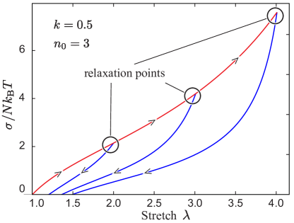
Figure 3: Stress-stretch responses of the Langevin chain system. Red and blue lines denote the stress-stretch relations during the stretching process and the de-stretching process, respectively.

III Non-ideal Mullins effect

In order to give a more realistic description of Mullins effect, in this section we will incorporate chain-length statistics, chain reattachment process, and chain entanglements into the model.

III.1 Chain-length distribution

The Langevin force model is highly non-linear in the moderate-to-large stretch range [evident in the $(1-x)$ denominator in $\mathcal{L}^{-1}(x)$] so we cannot simply assume all chains in the rubber have the same length. Here a log-normal distribution of the chain segment number in the prepared state (before any deformation), $n_{0}$, is assumed:

$$P(n_{0})=\frac{Z}{\sigma n_{0}}\exp\left[-\frac{(\ln n_{0}-\mu)^{2}}{2\sigma^{2}}\right]$$ (10)

with $\mu$ and $\sigma$ as the mean value and the standard variance of $\ln n_{0}$, respectively, and $Z$ as the normalisation factor. In addition, we denote $n^{\textmd{min}}_{0}$ as the minimal number of chain segments, the significance of which will be explained in the next sub-section. Note that the elongation factor $\eta(\lambda)$ will be different for chains with different initial lengths $n_{0}$, and this dependence is denoted by $\eta(\lambda,n_{0})$. Having these in mind we can re-write the energy density function and stress as

$$\begin{split}F_{\textmd{total}}(\lambda)&=\int_{n^{\textmd{min}}_{0}}^{\infty}P(n_{0})F[\lambda,\eta(\lambda,n_{0}),n_{0}]\mathrm{d}n_{0}\\ \sigma_{\textmd{total}}(\lambda)&=\int_{n^{\textmd{min}}_{0}}^{\infty}P(n_{0})\sigma[\lambda,\eta(\lambda,n_{0}),n_{0}]\mathrm{d}n_{0}.\end{split}$$ (11)

Computational details of the integral can be found in Appendix A. Here we define the elastic modulus, $W_{0}\equiv ZNk_{\textmd{B}}T/3$, as a fitting parameter in the following discussions.

III.2 Chain delamination during stretching

Evolution of the chain length distribution has been discussed in network models Dargazany and Itskov (2009); Itskov and Knyazeva (2016) and the main idea is that for a single non-Gaussian chain attached to a filler surface, there exists a maximum force $f_{\textmd{max}}$ beyond which the chain will break off from the filler aggregates. Here we argue instead that delamination starts when the force exerted on the chain reaches $f_{\textmd{max}}$, and stops only when the force is below $f_{\textmd{max}}$. The physical significance of $f_{\textmd{max}}$ can be thought of as the bonding force between a polymer segment and the aggregate surface with $f_{\textmd{max}}\cdot l$ as the bonding energy. The evolution of $\eta$ can be worked out as a function of $\lambda$ in the following manner.

The entropic force exerted by a Langevin chain with the end-to-end length as $r$ and the segment number as $n_{0}$ is Boyce and Arruda (2000):

$$f(r,n_{0})=\frac{k_{B}T}{l}\mathcal{L}^{-1}\left(\frac{r}{n_{0}l}\right).$$ (12)

By incorporating the relative elongation, $\eta(\lambda,n_{0})=n/n_{0}$ to allow chain elongation via delamination, the condition for non-delamination of the chain is given by:

$$\frac{k_{B}T}{l}\mathcal{L}^{-1}\left[\frac{\lambda}{\eta(\lambda,n_{0})\sqrt{n_{0}}}\right]\leq f_{\textmd{max}},$$ (13)

which can be re-expressed as,

$$\eta(\lambda,n_{0})\geq\frac{\lambda\nu}{\sqrt{n_{0}}},$$ (14)

with $1/{\nu}\equiv\mathcal{L}(\frac{f_{\textmd{max}}l}{k_{B}T})$. In the prepared state without any deformation, both $\lambda$ and $\eta$ are equal to one, and in this case equation (14) reduces to $n_{0}\geq\nu^{2}$. Then one can easily interpret $\nu^{2}$ as the minimum chain length in the material at the prepared state before any deformation, so we here define $n^{\textmd{min}}_{0}\equiv\nu^{2}$ and re-write equation (14) as

$$\eta(\lambda,n_{0})\geq\lambda\sqrt{\frac{n^{\textmd{min}}_{0}}{n_{0}}}\equiv\eta_{\textmd{d}}(\lambda,n_{0}).$$ (15)

In other words, when a chain with $n_{0}$ segments is stretched by $\lambda$, its $\eta$ will remain the same as long as $\eta\geq\eta_{\textmd{d}}$, and $\eta$ will become $\eta_{\textmd{d}}$ once the condition $\eta\geq\eta_{\textmd{d}}$ is not satisfied.

In practice, the exact force at which a chain delaminates from an aggregate surface may vary if considering the angle between the chain and normal direction of the aggregate surface, and the non-affine nature of the material. As a result, a smoothening scheme in varying $\eta$ is incorporated, which is shown in Figure 4. The degree of smoothening is given by a rate parameter $k_{\textmd{d}}$ and the $\eta$ evolution is governed by:

$$\begin{cases}\eta_{\textmd{ideal}}=\eta_{d}+\sqrt{\frac{n^{\textmd{min}}_{0}}{n_{0}}}/k_{\textmd{d}}\\ \mathrm{d}\eta/\mathrm{d}\lambda=0\qquad\qquad\qquad~{}~{}~{}~{}~{}\ \textrm{if}\ \eta>\eta_{\textmd{ideal}}\\ \mathrm{d}\eta/\mathrm{d}\lambda=k_{\textmd{d}}\cdot(\eta_{\textmd{ideal}}-\eta)\qquad\textrm{if}\ \eta<\eta_{\textmd{ideal}}\\ \end{cases}$$ (16)

for which more details are shown in Appendix B.

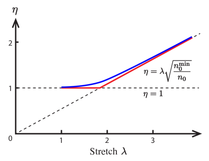
Figure 4: Evolution of $\eta$ with $\lambda$ starting from $(\eta=1,\lambda=1)$. Red solid line: evolution with no smoothening; blue solid line: evolution with smoothening.

III.3 Chain reattachment during relaxation

As the polymer network is relaxed from the stretched state (de-stretching process), the chains start coiling and some polymer segments can come close to the aggregate surface, re-forming polymer-aggregate bonds and resulting in partial recovery of the softening effect. We propose that the process of chain reattachment can only happen when the current stretch ratio during the de-stretching process is smaller than the residual stretch of the microcell (microcells have different residual stretches, depending on the initial chain length): the three-chain micro-cell has to be compressed, in short. Recalling equation (9) and setting the stress to be less than zero, we can obtain

$$\eta(\lambda,n_{0})\leq\frac{\lambda}{\sqrt{n_{0}}\mathcal{L}\left[\frac{1}{\sqrt{\lambda^{3}}}\mathcal{L}^{-1}\left(\frac{1}{\sqrt{\lambda n_{0}}}\right)\right]}\equiv\eta_{\textmd{r}}(\lambda,n_{0}).$$ (17)

Re-attachment commences when $\eta>\eta_{\textmd{r}}$, and here we assume the rate of change of $\eta$ is proportional to the difference between the current value $\eta$ and the ideal value $\eta_{\textmd{r}}$,

$$\mathrm{d}\eta/\mathrm{d}\lambda=k_{\textmd{r}}\cdot(\eta_{\textmd{r}}-\eta)\qquad\textmd{if}\ \eta>\eta_{\textmd{r}}$$ (18)

with $k_{\textmd{r}}$ the reattachment rate. The ideal Mullins effect has no reattachment and $k_{\textmd{r}}^{(\textmd{ideal})}=0$, while $k_{\textmd{r}}>0$ for non-ideal effects.

III.4 Entanglement correction

The final piece added to our model is a correction term arising from entanglement effects to address deviations at small $\lambda$. Here we borrow the entanglement terms from the general constitutive model Xiang et al. (2018, 2019); Zhong et al. (2019), which has energy density and stress:

$$\begin{split}W_{\textmd{e}}&=G_{\textmd{e}}\left(\frac{1}{\lambda}+2\sqrt{\lambda}\right)\\ \sigma_{\textmd{e}}&=G_{\textmd{e}}\left(-\frac{1}{\lambda^{2}}+\frac{1}{\sqrt{\lambda}}\right)\end{split}$$ (19)

The modulus $G_{\textmd{e}}$ is subject to damage of the form Zhong et al. (2019):

$$G_{\textmd{e}}=G_{\textmd{e0}}\exp\left[-\frac{k_{\textmd{e}}}{2}\left(\sqrt{I_{1}^{\textmd{max}}/3}-1\right)\right]$$ (20)

with $G_{\textmd{e0}}$ the initial entanglement modulus, $k_{\textmd{e}}$ the damage rate, and $I_{1}^{\textmd{max}}$ the maximum value of the first invariant of the Cauchy-green tensor ever attained in the material’s history. An illustration of how the entanglement correction contributes to the total stress can be found in Appendix C.

III.5 Numerical results

We fit our model to experimental data extracted from previous works Andriyana et al. (2015) as an example (table 1 shows parameters used) and Figure 5 shows how our model compares to experiment. A good agreement is achieved, especially for large stretch ratios, say $\lambda>2.5$, with strong initial non-linear responses for relaxation across all stretches as desired. Apart from the satisfactory fitting between our theory and the experiments, there are, however, also observable deviations at small stretches. For example, in Figure 6(a), the experimental data shows a ‘bump’ compared to our theoretical result during the stretching process. One way to incorporate such ‘bumpy’ behaviours is by the addition of aggregate elasticity Dargazany and Itskov (2013), which is not considered in the current work to keep the relative transparency of the theory.

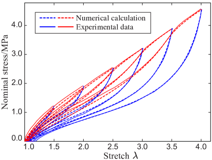
Figure 5: Comparison of our model (dashed lines) to experimental data (solid lines) Andriyana et al. (2015). Red and blue lines denote the stress-stretch relations during the stretching process and the de-stretching process, respectively.

Table 1: Fitting parameters

Parameter	Description	Value
$W_{\textmd{0}}$	Elastic modulus	0.072 (MPa)
$n^{\textmd{min}}_{0}$	Minimum chain length	1.17
$k_{\textmd{d}}$	Delamination rate	6
$k_{\textmd{r}}$	Reattachment rate	8
$\mu$	Log-Normal parameter 1	2.8
$\sigma$	Log-Normal parameter 2	1.6
$G_{\textmd{e0}}$	Entanglement modulus	1.1(MPa)
$k_{\textmd{e}}$	Entanglement damage	2.5

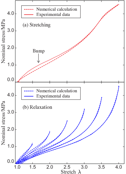
Figure 6: Stress-stretch relations for (a) stretching process and (b) de-stretching process.

IV Conclusion

To conclude, we have developed a physical model to understand the non-ideal Mullins effect ubiquitously observed in filled rubber elastomers, by incorporating both chain delamination from and chain reattachment to the filled aggregates. Good agreements can be obtained between the model calculation and experimental data. We believe this portable theory can be easily adapted to meet more practical needs and utilised in analysing mechanic properties of polymer nano-/micro-composites.

Appendix A Integration method

The integration in equation (11) extends to infinity and traditionally a large-n cutoff will be used in the integration so that the integration range covers 95% of the chains. In the actual computation, however, we observe that the chains assume the Gaussian behaviour at large $n$ and delamination only occurs for $n_{0}$ up to $n_{0}\sim\lambda_{\textmd{max}}^{2}\sim 16$, so the stress contribution becomes independent of $n_{0}$ and can be taken out of the integral.

Expanding $\mathcal{L}^{-1}(x)$ to third order we have $\mathcal{L}^{-1}(x)\approx 3x+0.1x^{2}+1.09x^{3}...$and since $x\sim 1/\sqrt{n}$, with a cut-off $n_{\mathrm{max}}=50$ and truncating the series to first order, the fractional error in $\mathcal{L}^{-1}(x)$ is $\sim(0.1x+x^{2})/3\sim 1.2\%$, similar to the accuracy achieved by the R. Jedynak approximation. The nominal stress calculation can then be written as

$$\begin{split}\sigma_{\textmd{total}}(\lambda)\approx&\int_{n_{0}^{\mathrm{min}}}^{50}P(n_{0})\sigma[\lambda,\eta(\lambda,n_{0}),n_{0}]\mathrm{d}n_{0}\\ +&Nk_{\textmd{B}}T\left(\lambda-\frac{1}{\lambda^{2}}\right)\cdot\int_{50}^{\infty}P(n_{0})\mathrm{d}n_{0},\end{split}$$ (21)

and the integration from $50$ to $\infty$ can be computed with Mathematica. The first integration has to be done numerically and 10,000 points are used in our simulation.

Appendix B Smoothening of $\eta$ evolution

The smoothening procedure for $\eta$ during delamination is similar to equation (18). We start by solving the following simplified model for $y(x)$ and $y_{\textmd{ideal}}(x)$

$$\begin{cases}y_{\textmd{ideal}}(x)=\alpha x\\ \frac{\mathrm{d}y(x)}{\mathrm{d}x}=\beta[y_{\textmd{ideal}}(x)-y(x)]\\ y(0)=0\end{cases}$$ (22)

which has solution $y(x)=\alpha x-\frac{\alpha}{\beta}(1-e^{-\beta x})$. Note that the solution asymptotically approaches $\alpha x-\frac{\alpha}{\beta}$ instead of $y_{\textmd{ideal}}(x)$, so $y_{\textmd{ideal}}(x)$ has to be shifted upwards by $\frac{\alpha}{\beta}$ for $y(x)$ to approach $\alpha x$. Going back to our $\eta-\lambda$ system we can make the identification $(x,y)=(0,0)\rightarrow(\lambda,\eta)=\left(\sqrt{\frac{n_{0}}{n^{\textmd{min}}_{0}}},1\right)$, $\alpha\rightarrow\sqrt{\frac{n^{\textmd{min}}_{0}}{n_{0}}}$ and $\beta\rightarrow k_{d}$, so the evolution law has the following form:

$$\begin{cases}\eta_{\textmd{ideal}}=\eta_{r}+\sqrt{\frac{n^{\textmd{min}}_{0}}{n_{0}}}/k_{\textmd{d}}\\ \mathrm{d}\eta/\mathrm{d}\lambda=0\qquad\qquad\qquad\qquad\qquad\ &\textmd{if}\ \eta>\eta_{\textmd{ideal}}\\ \mathrm{d}\eta/\mathrm{d}\lambda=k_{\textmd{d}}\cdot(\eta_{\textmd{ideal}}-\eta)&\textmd{if}\ \eta<\eta_{\textmd{ideal}}\\ \end{cases}$$ (23)

Appendix C Entanglement contribution

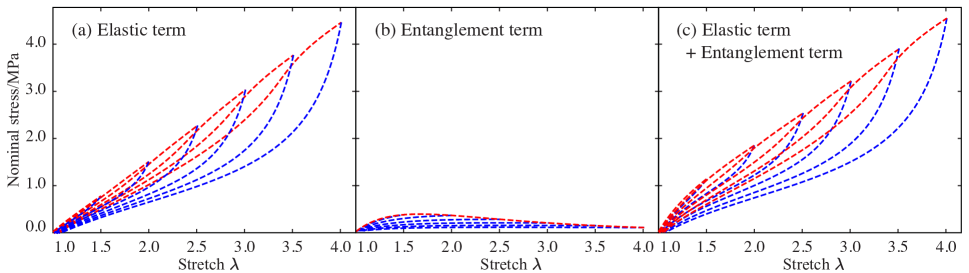
Figure 7: Stress-stretch relations for considering only (a) the elastic term and (b) the entanglement term. (c) Stress-stretch relations for adding the contributions of both the elastic term and the entanglement term. Red and blue lines denote the stress-stretch relations during the stretching process and the de-stretching process, respectively.

Figure 7 shows separately how the elastic term and entanglement term each contribute to the total stress. Although the fitting parameter for the elastic term is much smaller than the entanglement term, the rapidly-increasing inverse Langevin function meant that the elastic contribution still dominates. With only elastic term [Figure 7(a)] the initial stress-stretch response appears linear due to the averaging effect of integrating over all chain lengths, and the entanglement term [Figure 7(b)] adds a bump at the start to match the experimental observation.

References

- Vilgis et al. (2009) T. A. Vilgis, G. Heinrich, and M. Klüppel, Reinforcement of polymer nano-composites: theory, experiments and applications (Cambridge University Press, 2009).
- Saheb and Jog (1999) D. N. Saheb and J. P. Jog, Natural fiber polymer composites: a review, Advances in Polymer Technology: Journal of the Polymer Processing Institute 18, 351 (1999).
- Ku et al. (2011) H. Ku, H. Wang, N. Pattarachaiyakoop, and M. Trada, A review on the tensile properties of natural fiber reinforced polymer composites, Composites Part B: Engineering 42, 856 (2011).
- Sanjay et al. (2018) M. Sanjay, P. Madhu, M. Jawaid, P. Senthamaraikannan, S. Senthil, and S. Pradeep, Characterization and properties of natural fiber polymer composites: A comprehensive review, Journal of Cleaner Production 172, 566 (2018).
- Donnet (2003) J. Donnet, Nano and microcomposites of polymers elastomers and their reinforcement, Composites science and technology 63, 1085 (2003).
- Mohammed et al. (2015) L. Mohammed, M. N. Ansari, G. Pua, M. Jawaid, and M. S. Islam, A review on natural fiber reinforced polymer composite and its applications, International Journal of Polymer Science 2015 (2015).
- Sanjay et al. (2016) M. Sanjay, G. Arpitha, L. L. Naik, K. Gopalakrishna, and B. Yogesha, Applications of natural fibers and its composites: An overview, Natural Resources 7, 108 (2016).
- Mu et al. (2007) Q. Mu, S. Feng, and G. Diao, Thermal conductivity of silicone rubber filled with zno, Polymer composites 28, 125 (2007).
- Ramnath et al. (2014) B. V. Ramnath, C. Elanchezhian, M. Jaivignesh, S. Rajesh, C. Parswajinan, and A. S. A. Ghias, Evaluation of mechanical properties of aluminium alloy–alumina–boron carbide metal matrix composites, Materials & Design 58, 332 (2014).
- Ren and Cornish (2019) X. Ren and K. Cornish, Eggshell improves dynamic properties of durable guayule rubber composites co-reinforced with silanized silica, Industrial Crops and Products 138, 111440 (2019).
- Choi et al. (2018) S.-S. Choi, H.-M. Kwon, Y. Kim, E. Ko, and K.-S. Lee, Hybrid factors influencing wet grip and rolling resistance properties of solution styrene-butadiene rubber composites, Polymer International 67, 340 (2018).
- Kim et al. (2019) M. C. Kim, J. Adhikari, J. K. Kim, and P. Saha, Preparation of novel bio-elastomers with enhanced interaction with silica filler for low rolling resistance and improved wet grip, Journal of Cleaner Production 208, 1622 (2019).
- Mars and Fatemi (2002) W. Mars and A. Fatemi, A literature survey on fatigue analysis approaches for rubber, International Journal of fatigue 24, 949 (2002).
- Bathias (2006) C. Bathias, An engineering point of view about fatigue of polymer matrix composite materials, International journal of fatigue 28, 1094 (2006).
- Dong et al. (2014) B. Dong, C. Liu, and Y.-P. Wu, Fracture and fatigue of silica/carbon black/natural rubber composites, Polymer Testing 38, 40 (2014).
- Ramakrishna et al. (2001) S. Ramakrishna, J. Mayer, E. Wintermantel, and K. W. Leong, Biomedical applications of polymer-composite materials: a review, Composites science and technology 61, 1189 (2001).
- Diani et al. (2009) J. Diani, B. Fayolle, and P. Gilormini, A review on the mullins effect, European Polymer Journal 45, 601 (2009).
- Mullins (1948) L. Mullins, Effect of stretching on the properties of rubber, Rubber Chemistry and Technology 21, 281 (1948).
- Blanchard and Parkinson (1952) A. Blanchard and D. Parkinson, Breakage of carbon-rubber networks by applied stress, Rubber Chemistry and Technology 25, 808 (1952).
- Houwink (1956) R. Houwink, Slipping of molecules during the deformation of reinforced rubber, Rubber Chemistry and Technology 29, 888 (1956).
- Kraus et al. (1966) G. Kraus, C. Childers, and K. Rollmann, Stress softening in carbon black-reinforced vulcanizates. strain rate and temperature effects, Journal of Applied Polymer Science 10, 229 (1966).
- Hanson et al. (2005) D. E. Hanson, M. Hawley, R. Houlton, K. Chitanvis, P. Rae, E. B. Orler, and D. A. Wrobleski, Stress softening experiments in silica-filled polydimethylsiloxane provide insight into a mechanism for the mullins effect, Polymer 46, 10989 (2005).
- Varol et al. (2020) H. S. Varol, A. Srivastava, S. Kumar, M. Bonn, F. Meng, and S. H. Parekh, Bridging chains mediate nonlinear mechanics of polymer nanocomposites under cyclic deformation, Polymer , 122529 (2020).
- Boyce and Arruda (2000) M. C. Boyce and E. M. Arruda, Constitutive models of rubber elasticity: a review, Rubber chemistry and technology 73, 504 (2000).
- Wang and Guth (1952) M. C. Wang and E. Guth, Statistical theory of networks of non-gaussian flexible chains, The Journal of Chemical Physics 20, 1144 (1952).
- Meng and Terentjev (2017) F. Meng and E. M. Terentjev, Theory of semiflexible filaments and networks, Polymers 9, 52 (2017).
- Meng and Terentjev (2016) F. Meng and E. M. Terentjev, Nonlinear elasticity of semiflexible filament networks, Soft Matter 12, 6749 (2016).
- Andriyana et al. (2015) A. Andriyana, M. S. Loo, G. Chagnon, E. Verron, and S. Y. Ch’ng, Modeling the mullins effect in elastomers swollen by palm biodiesel, International Journal of Engineering Science 95, 1 (2015).
- Chagnon et al. (2004) G. Chagnon, E. Verron, L. Gornet, G. Marckmann, and P. Charrier, On the relevance of continuum damage mechanics as applied to the mullins effect in elastomers, Journal of the Mechanics and Physics of Solids 52, 1627 (2004).
- Dargazany and Itskov (2009) R. Dargazany and M. Itskov, A network evolution model for the anisotropic mullins effect in carbon black filled rubbers, International Journal of Solids and Structures 46, 2967 (2009).
- Kuhn and Grün (1942) W. Kuhn and F. Grün, Beziehungen zwischen elastischen konstanten und dehnungsdoppelbrechung hochelastischer stoffe, Kolloid-Zeitschrift 101, 248 (1942).
- Jedynak (2015) R. Jedynak, Approximation of the inverse langevin function revisited, Rheologica Acta 54, 29 (2015).
- Itskov and Knyazeva (2016) M. Itskov and A. Knyazeva, A rubber elasticity and softening model based on chain length statistics, International Journal of Solids and Structures 80, 512 (2016).
- Xiang et al. (2018) Y. Xiang, D. Zhong, P. Wang, G. Mao, H. Yu, and S. Qu, A general constitutive model of soft elastomers, Journal of the Mechanics and Physics of Solids 117, 110 (2018).
- Xiang et al. (2019) Y. Xiang, D. Zhong, P. Wang, T. Yin, H. Zhou, H. Yu, C. Baliga, S. Qu, and W. Yang, A physically based visco-hyperelastic constitutive model for soft materials, Journal of the Mechanics and Physics of Solids 128, 208 (2019).
- Zhong et al. (2019) D. Zhong, Y. Xiang, T. Yin, H. Yu, S. Qu, and W. Yang, A physically-based damage model for soft elastomeric materials with anisotropic mullins effect, International Journal of Solids and Structures 176, 121 (2019).
- Dargazany and Itskov (2013) R. Dargazany and M. Itskov, Constitutive modeling of the mullins effect and cyclic stress softening in filled elastomers, Physical Review E 88, 012602 (2013).