Abstract.

Through tropical normal idempotent matrices, we introduce isocanted alcoved polytopes, computing their $f$–vectors and checking the validity of the following five conjectures: Bárány, unimodality, $3^{d}$, flag and cubical lower bound (CLBC). Isocanted alcoved polytopes are centrally symmetric, almost simple cubical polytopes. They are zonotopes. We show that, for each dimension, there is a unique combinatorial type. In dimension $d$, an isocanted alcoved polytope has $2^{d+1}-2$ vertices, its face lattice is the lattice of proper subsets of $[d+1]$ and its diameter is $d+1$. They are realizations of $d$–elementary cubical polytopes. The $f$–vector of a $d$–dimensional isocanted alcoved polytope attains its maximum at the integer $\lfloor d/3\rfloor$.

Keywords: cubical polytope, isocanted, alcoved, centrally symmetric, almost simple, zonotope, $f$–vector, cubical $g$–vector, unimodal, flag, face lattice, log–concave sequence, tropical normal idempotent matrix, symmetric matrix.

MSC 2010: 52B12, 15A80

1. Introduction

This paper deals with $f$–vectors of isocanted alcoved polytopes. A polytope is the convex hull of a finite set of points in $\mathbb{R}^{d}$. A polytope is a box if its facets are only of one sort: $x_{i}=cnst$, $i\in[d]$. A polytope is alcoved if its facets are only of two sorts: $x_{i}=cnst$ and $x_{i}-x_{j}=cnst$, $i,j\in[d]$, $i\neq j$. Every alcoved polytope can be viewed as the perturbation of a box. In a box we distinguish two opposite vertices and the perturbation consists on canting (i.e., beveling, meaning producing a flat face upon something) some (perhaps all) of the $(d-2)$–faces of the box not meeting the distinguished vertices. When the perturbation happens for all such $(d-2)$–faces and with the same positive magnitude, we obtain as a result an isocanted alcoved polytope. The notion makes sense only for $d\geq 2$.

The $f$–vector of a $d$–polytope $\mathcal{P}$ is the tuple $(f_{0},f_{1},\ldots,f_{d-1})$, where $f_{j}$ is the number of $j$–dimensional faces in $\mathcal{P}$, for $j=0,1,2,\ldots,{d-1}$. The $f$–vector can be extended with $f_{d}=1$. It is well known that the $f$–vector of a $d$–box is

(1.1) $$B_{d,j}=2^{d-j}{d\choose j},\quad j=0,1,\ldots,d.$$

The quest for $f$–vectors is unrelenting. As Ziegler writes in [40] “on some fundamental problems embarrassingly little progress was made; one notable such problem concerns the shapes of $f$–vectors”and “new polytopes with interesting $f$–vectors should be produced”and also “it seems that overall, we are short of examples.”

The main result in this paper is that the $f$–vector of an isocanted $d$–alcoved polytope is given by

(1.2) $$I_{d,j}=(2^{d+1-j}-2){{d+1}\choose{j}},\ j=0,1,\ldots,d-1,\quad I_{d,d}=1.$$

The numbers $I_{d,j}$ are even, for $j\leq d-1$, because isocanted alcoved $d$–polytopes are centrally symmetric. We verify several conjectures for $f$–vectors, namely, unimodality, Bárány, Kalai $3^{d}$ and flag conjectures as well as CLCB. Further properties are proved, showing that isocanted alcoved polytopes are $d$–elementary cubical, almost simple and zonotopes.

The paper is organized as follows. In section 3 we give the definition and then, in Theorem 3.4, we prove a crucial characterization: isocanted alcoved polytopes are those alcoved polytopes having a unique vertex for each proper subset of $[d+1]$. Concrete examples are given in Example 3.5. It follows from Theorem 3.4 that the face lattice of an isocanted alcoved $d$–polytope is the lattice of proper subsets of $[d+1]$. It is proved that isocanted alcoved polytopes are cubical and are zonotopes. In section 4 we explain in detail the cases of dimensions 3 and 4, providing figures which help the reader visualize the many properties of these polytopes. We compute two invariants of 4–isocanted alcoved polytopes: fatness and $f_{03}$. In section 5 we prove that the five mentioned conjectures hold true for isocanted alcoved polytopes. Log–concavity provides a short proof of the unimodality of $I_{d,j}$, for fixed $d\geq 2$. We also prove that the maximum of $I_{d,j}$ is attained at the integer $\lfloor\frac{d}{3}\rfloor$. We show that the diameter is $d+1$.

This paper encompasses tropical matrices and classical polytopes, in the sense that tropical matrices are the means to describe certain polytopes. We use several sorts of special matrices, operated with tropical addition $\oplus=\max$ and tropical multiplication $\odot=+$, such as: normal idempotent (with respect to $\odot$), visualized normal idempotent matrices, symmetric normal idempotent matrices and, among these, box matrices, cube matrices and isocanted matrices.

Tropical linear algebra and tropical algebraic geometry are fascinating, new, fast growing areas of mathematics with new and important results. For our purposes we recommend [8, 9, 10, 11, 21, 22, 23, 27, 34] among many others. Alcoved polytopes have been first studied in [20, 37], then in [24, 26]. Cubical polytopes have been addressed in [1, 2, 5, 6, 17]. General references for polytopes are [3, 4, 13, 19, 29, 33, 39, 40]. Normal idempotent matrices have been used in [26, 38]. Idempotent matrices, also called Kleene stars, have been used in [24, 30, 36] in connection to polytopes.

2. Background and notations

Well–known definitions and facts are presented here. The set $\{1,2,\ldots,d+1\}$ is denoted $[d+1]$ and ${{[d+1]}\choose j}$ denotes the family of subsets of $[d+1]$ of cardinality $j$. The origin in $\mathbb{R}^{d}$ is denoted ${\bf{0}}$. Maximum and minimum are taken componentwise in $\mathbb{R}^{d}$. A polyhedron in $\mathbb{R}^{d}$ is the intersection of a finite number of halfspaces. It may be unbounded. A bounded polyhedron is called a polytope and every polytope is the convex hull of a finite set of points. A $d$–polyhedron is a polyhedron of dimension $d$. A $d$–polyhedron $\mathcal{P}$ is alcoved if its facets are only of two types: $x_{i}=cnst$ and $x_{i}-x_{j}=cnst$, $i,j\in[d]$, $i\neq j$. A double index notation is useful here because, in this way, we can gather the coefficients in a matrix over $\mathbb{R}\cup\{\pm\infty\}$: indeed, write

(2.1) $$a_{i,j}\leq x_{i}-x_{j}\leq-a_{j,i}$$

and, similarly,

(2.2) $$a_{i,d+1}\leq x_{i}\leq-a_{d+1,i}.$$

Then, setting $a_{i,j}=\pm\infty$ if one facet $x_{i}-x_{j}=cnst$ is not specified, and letting (by convention) $a_{i,i}=0$, for all $i\in[d+1]$, we get a square matrix $A=[a_{i,j}]\in M_{d+1}(\mathbb{R}\cup\{\pm\infty\})$ from $\mathcal{P}$. We write $\mathcal{P}=\operatorname{p}(A)$ to express the former relationship between the polyhedron $\mathcal{P}$ and the matrix $A$. In addition to $a_{i,i}=0,i\in[d+1]$, the entries of the matrix $A$ satisfy $-\infty\leq a_{i,j}\leq-a_{j,i}\leq+\infty$, for all $i,j\in[d+1]$. Different matrices $A$ may give rise to the same polyhedron.

Definition 2.1 (Alcoved polytope (AP)).

A $d$–polytope $\mathcal{P}\subset\mathbb{R}^{d}$ is alcoved if there exist constants $a_{i,j}\in\mathbb{R}$ such that $x\in\mathcal{P}$ if and only if $a_{i,d+1}\leq x_{i}\leq-a_{d+1,i}$, for all $i\in[d]$, and $a_{i,j}\leq x_{i}-x_{j}\leq-a_{j,i}$, for all $i,j\in[d+1]$. Letting $A=[a_{i,j}]\in M_{d+1}(\mathbb{R})$, we write $\mathcal{P}=\operatorname{p}(A)$.

Important particular cases provide special matrices as follows:

1. ${\bf{0}}\in\operatorname{p}(A)$ if and only if $A$ is normal (N) (meaning $a_{i,i}=0,a_{i,j}\leq 0,\forall i,j$), (see [10, 38])

2. if ${\bf{0}}\in\operatorname{p}(A)$, then $A$ describes $\operatorname{p}(A)$ optimally (or tightly) if and only if $A$ is normal idempotent (NI) (meaning that, in addition to normality, we have $A\odot A=A$, which requires that $a_{i,j}+a_{jk}\leq a_{ik},\forall i,j,k$) (see [24, 30, 36]).

3. for each alcoved polytope $\mathcal{P}$ containing ${\bf{0}}$ there exist a unique NI matrix $A$ such that $\mathcal{P}=\operatorname{p}(A)$ (see Lemma 2.6 in [24] and [30, 36]).

Combinatorial properties of polytopes are, by nature, translation invariant. Every translate of an alcoved polytope is alcoved. For each general alcoved polytope $\mathcal{P}$, infinitely many translates $\mathcal{P}^{\prime}$ of $\mathcal{P}$ exist such that ${\bf{0}}\in\mathcal{P}^{\prime}$. We can choose any such $\mathcal{P}^{\prime}$ to study $\mathcal{P}$, and we know that $\mathcal{P}^{\prime}=\operatorname{p}(A)$ for a unique NI matrix $A$. Often, we choose $\mathcal{P}^{\prime}$ in two special locations with respect to ${\bf{0}}$, each location corresponding to a subclass of NI matrices:

1. ${\bf{0}}=\max\operatorname{p}(A)$ if and only if $A$ is visualized normal idempotent (VNI) (in addition to NI, the entries of $A$ satisfy $a_{d+1,i}=0,\forall i$), (see [10, 24, 26])

2. $\operatorname{p}(A)=-\operatorname{p}(A)$ if and only if $A$ is symmetric normal idempotent (SNI) (in addition to NI, the entries of $A$ satisfy $a_{i,j}=a_{j,i},\forall i,j$), (see [16, 26]).

From [26], we know that translation of an alcoved polyhedron $\operatorname{p}(A)$ corresponds to conjugation of its matrix $A$ by a diagonal matrix (with null last diagonal entry).

Our aim is, after defining isocanted alcoved polytopes, to compute the $f$–vector of those. But, what is already known about vertices of an alcoved polytope $\operatorname{p}(A)$ in $\mathbb{R}^{d}$? First, the number of vertices of $\operatorname{p}(A)$ is bounded above by ${2d}\choose{d}$ and this bound is sharp (see [11, 34]). Which points are vertices of $\operatorname{p}(A)$? In order to answer this question we introduce (a) the auxiliary matrix $A_{0}$ and (b) the notion of tropical linear subspace (by linear, we mean affine linear.)

For $A=[a_{i,j}]$, the matrix $A_{0}=[\alpha_{i,j}]$ is defined by $\alpha_{i,j}:=a_{i,j}-a_{d+1,j}=a_{i,j}\odot(-a_{d+1,j})$. The columns in $A_{0}$ are scalar multiples (with respect to $\odot$) of the columns in $A$. The fact that $\operatorname{diag}(A)$ is zero implies that $\operatorname{row}(d+1,A_{0})$ is zero (and conversely), so that the columns in $A_{0}$ belong to the hyperplane $\{x\in\mathbb{R}^{d+1}:x_{d+1}=0\}$ which is identified with $\mathbb{R}^{d}$. Besides, if $A$ is NI, then $A=A_{0}$ if and only if $A$ is VNI.

Inequalities (2.2) are transformed into

(2.3) $$\alpha_{i,d+1}\leq x_{i}\leq\alpha_{i,i},\ \forall i\in[d]$$

which yield the following facts

(2.4) $$\min\operatorname{p}(A)=\operatorname{col}(d+1,A_{0}),\qquad\max\operatorname{p}(A)=\operatorname{diag}(A_{0}).$$

Besides, $\operatorname{p}(A)$ is the family of all tropical affine combinations of columns of $A_{0}$ (see Theorem 2.1[24], Proposition 12 [36])

(2.5) $$\operatorname{p}(A)=\{x\in\mathbb{R}^{d+1}:x_{d+1}=0,x=\lambda_{1}\odot\operatorname{col}(1,A_{0})\oplus\cdots\oplus\lambda_{d+1}\odot\operatorname{col}(d+1,A_{0}),\lambda_{j}\in\mathbb{R},0=\lambda_{1}\oplus\cdots\oplus\lambda_{d+1}\}.$$

$\operatorname{p}(A)$ is a proper subset of the unique linear subspace determined by the columns of $A_{0}$. In particular, the columns of $A_{0}$ are some of the vertices of $\operatorname{p}(A)$. They are called the generators of $\operatorname{p}(A)$. The rest of vertices of $\operatorname{p}(A)$ are tropical linear combinations of the generators, and are thus called generated vertices of $\operatorname{p}(A)$. In order to explain this, we must first define tropical linear subspaces. A tropical linear subspace is the tropicalization of a linear subspace of $K^{d}$, where $K:=\mathbb{C}\{\{t\}\}$ is the field of Puiseux series. If $L\subseteq K^{d}$ is a linear subspace and $I(L)\subseteq K[x_{1}^{\pm 1},x_{2}^{\pm 1},\ldots,x_{d}^{\pm 1}]$ is the ideal of all Laurent polynomials vanishing on $L$, consider $q\in I(L)$, $q=\sum_{s\in S}a_{s}\textbf{x}^{s}$, with $\textbf{x}=(x_{1},x_{2},\ldots,x_{d})$ variables, $s=(s_{1},s_{2},\ldots,s_{d})\in S$ exponents, $S\subset\mathbb{N}^{d}$ a finite set, $a_{s}\in K$ and $\textbf{x}^{s}=x_{1}^{s_{1}}x_{2}^{s_{2}}\cdots x_{d}^{s_{d}}$. Then, consider the tropicalization of $q$

(2.6) $$\operatorname{Trop}(q):=\bigoplus_{s\in S}-\operatorname{v}(a_{s})\odot x_{1}{s_{1}}\odot x_{2}{s_{2}}\odot\cdots\odot x_{d}{s_{d}}=\max_{s\in S}-\operatorname{v}(a_{s})+x_{1}{s_{1}}+x_{2}{s_{2}}+\cdots+x_{d}{s_{d}}$$

where tropical powers are transformed into products, $\operatorname{v}:K\setminus\{0\}\rightarrow\mathbb{Q}$ is the standard valuation (i.e., the order of vanishing of a series). The corner locus of $\operatorname{Trop}(q)$ is, by definition, the collection of points $x\in\mathbb{R}^{d}$ where the maximum in $\operatorname{Trop}(q)(x)$ is attained, at least, twice. Finally $\operatorname{Trop}(L)$ is, by definition, the closure of the intersection of corner loci, for all $q\in I(L)$. Since the corner locus of $\operatorname{Trop}(q)$ is piecewise linear, then tropical linear subspaces are polyhedral complexes.

Notice that a unique tropical linear subspace is determined by each subset of generators (i.e., of columns of $A_{0}$). A convenient notation is $L_{A}(W)$, for each $W\in{{[d+1]}\choose{j}}$ with $1\leq j\leq d$. We will write $L(W)$, when $A$ is understood. $L(W)$ is a $(j-1)$–dimensional tropical linear subspace and, being piecewise linear, the subspace $L(W)$ has a finite number of vertices (however, an upper bound on how many is not known in all cases; see [34]). Returning to the question of which points are vertices of $\operatorname{p}(A)$, the answer is that the vertices of $\operatorname{p}(A)$ are all the vertices of all subspaces $L(W)$, for $W\in{{[d+1]}\choose{j}}$. The case $j=1$ gives the $d+1$ generators of $\operatorname{p}(A)$.

The easiest alcoved polytopes are boxes and cubes, determined by equations $x_{i}=cnst$. We fix a convenient matrix notation for boxes with special matrices VNI and SNI (see Items 1 and 2 in p. 1). Recall that translation of an alcoved polyhedron $\operatorname{p}(A)$ is achieved by conjugation of matrix $A$.

Notation 2.2 (Box matrices).

Given real numbers $\ell_{i}>0$, $i\in[d]$, consider

1. $B^{VNI}(d+1;\ell_{1},\ell_{2},\ldots,\ell_{d})=[b_{i,j}]\in M_{d+1}(\mathbb{R})$ with $b_{i,j}=\begin{cases}-\ell_{i},&d+1\neq i\neq j,\\ 0,&\text{ otherwise,}\\ \end{cases}$. This matrix is VNI (easily checked) and called the VNI box matrix with edge–lengths $\ell_{j}$. In particular, we have the VNI cube matrix $Q^{VNI}(d+1;\ell):=B^{VNI}(d+1;\ell,\ldots,\ell)$.

2. The conjugate matrix $D\odot B^{VNI}(d+1;\ell_{1},\ell_{2},\ldots,\ell_{d})\odot D^{-1}$ is SNI (easily checked), where $D=\operatorname{diag}(\ell_{1}/2,\ell_{2}/2,\ldots,\ell_{d}/2,0)$. It is denoted $B^{SNI}(d+1;\ell_{1},\ell_{2},\ldots,\ell_{d})=[c_{i,j}]$ and we have $c_{i,j}=\begin{cases}-\ell_{i}/2,&j=d+1,\\ -\ell_{j}/2,&i=d+1,\\ 0,&i=j,\\ (-\ell_{i}-\ell_{j})/2,&\text{otherwise.}\\ \end{cases}$ Similarly we have the cube matrix $Q^{SNI}(d+1;\ell)$.

3. A box matrix is any diagonal conjugate of the above, i.e., $D^{\prime}\odot B\odot{D^{\prime}}^{-1}$, where $D^{\prime}=\operatorname{diag}(d^{\prime}_{1},d^{\prime}_{2},\ldots,d^{\prime}_{d},0)$ with $d^{\prime}_{j}\in\mathbb{R}$ and $B=B^{VNI}(d+1;\ell_{1},\ell_{2},\ldots,\ell_{d})$. It is NI (easily checked).

Definition 2.3 (from de la Puente [26]).

Any non–positive real matrix $E\in M_{d+1}(\mathbb{R})$ with null diagonal, last row and column is called perturbation matrix. In symbols, $E=[e_{i,j}]$ with $e_{i,i}=e_{d+1,i}=e_{i,d+1}=0$ and $e_{i,j}\leq 0,\forall i,j$.

In [26] it is proved that for any NI matrix $A\in M_{d+1}(\mathbb{R})$ (not necessarily VNI or SNI), there exists a unique decomposition $A=B-E$, where $B$ is a NI box matrix and $E$ is a perturbation matrix. The polytope $\operatorname{p}(B)$ is called the bounding box of the alcoved polytope $\operatorname{p}(A)$. It is also proved that $E$ is invariant under conjugation by diagonal matrices with zero last diagonal entry.

3. Definition, characterization and $f$–vector of IAPs

Definition 3.1 (Isocanted alcoved polytope (IAP)).

Let $A\in M_{d+1}(\mathbb{R})$ be a NI matrix with decomposition $A=B-E$. The alcoved polytope $\operatorname{p}(A)$ is isocanted if $E$ is a constant perturbation matrix, i.e., there exists $a>0$ such that $e_{i,j}=-a$, for all $i,j\in[d]$, $i\neq j$. The number $a$ is called cant parameter of $\operatorname{p}(A)$. We write $E=[-a]$, by abuse of notation.

Remark 3.2.

Every box in $\mathbb{R}^{d}$ is centrally symmetric and, by a translation, we can place its center of symmetry at the origin of $\mathbb{R}^{d}$. An IAP is a perturbed box with constant (whence symmetric) matrix $E$. Then, every IAP is centrally symmetric,by Item 2 in p. 2.

Notation 3.3 (Special matrices for visualized IAPs and symmetric IAPs, with cubic bounding boxes).

Given real numbers $a,\ell$, consider the constant perturbation matrix $E=[-a]\in M_{d+1}(\mathbb{R})$ as above and the matrices (as in Notation 2.2)

1. $I^{VNI}(d+1;\ell,a):=Q^{VNI}(d+1;\ell)-E$,

2. $I^{SNI}(d+1;\ell,a):=Q^{SNI}(d+1;\ell)-E$.

It is an easy computation to check that, for these matrices to be NI, it is necessary and sufficient that $0<a<\ell$.

The following is the crucial step of the paper. Its proof contains the only tropical computations in what follows.

Theorem 3.4 (Characterization of IAPs).

An alcoved $d$–polytope $\mathcal{P}=\operatorname{p}(A)$ is isocanted if and only if, for each ${1}\leq j\leq d$ and each $W\in{{[d+1]}\choose{j}}$ , the tropical linear subspace $L_{A}(W)$ has a unique vertex.

Proof.

Without loss of generality, we can assume that the bounding box of $\mathcal{P}$ is a cube (of edge–length $\ell>0$) since an affine bijection does not affect the result. We can also assume that $\mathcal{P}$ is located in $d$–space so that ${\bf{0}}=\max\mathcal{P}$, because a translation does not affect the result. Then $\mathcal{P}=\operatorname{p}(C)$, with $C=Q^{VNI}(d+1;\ell)-E$, for some positive $\ell$, as in in Notation 2.2 and Definition 2.3. For $W\subset[d+1]$, let $C(W)$ denote the $(d+1)\times j$ sized matrix whose columns are indexed by $W$ and taken from $C$.

$(\Rightarrow)$ Assume $\mathcal{P}$ is IAP. Then $E=[-a]$ is constant and then $C=I^{VNI}(d+1;\ell,a)=[c_{i,j}]$, as in Item 1 of Notation 3.3. In symbols, $c_{i,j}=\begin{cases}-\ell,&i\neq j=d+1,\\ 0,&i=j\text{ or }i=d+1,\\ -\ell+a,&\text{otherwise,}\\ \end{cases}$  with $0<a<\ell$. Note that the tropical rank of $C$ is $d+1$ (meaning that the maximum in the tropical permanent of $C$ is attained only once.) In particular, $\operatorname{rk}_{\operatorname{tr}}C(W)=j$, for each proper subset $W\in{{[d+1]}\choose{j}}$.

For $j=1$, $L(W)$ reduces to a point (a generator) and uniqueness is trivial. Consider a point $x\in\mathbb{R}^{d+1}$ with $x_{d+1}=0$, and let $C(W,x)$ be the matrix $C(W)$ extended with column $x$. It is well–known (see [27, 34, 35]) that $x\in L(W)$ if and only if $\operatorname{rk}_{\operatorname{tr}}C(W,x)\leq j$, (meaning that the maximum in each order $(j+1)$ tropical minor is attained, at least, twice). Besides, $x$ is a vertex in $L(W)$ if and only if the maximum in each order $(j+1)$ tropical minor of $C(W,x)$ is attained $(j+1)$ times. Indeed, the vertices of $L(W)$ are got by computing the corner locus of $L(W)$, then the corner locus of the corner locus, repeatedly. Each iteration reduces the dimension of the computed set, because points where the maxima are attained one more time than previously, are computed.

For each $2\leq j\leq d$ and each index family $1\leq i_{1}<i_{2}<\cdots<i_{j}\leq d+1$, let $m_{i_{1},i_{2},\ldots,i_{j}}$ (resp. $m_{i_{1},i_{2},\ldots,i_{j}}(x)$) denote the order $j$ minor of $C(W)$ (resp. $C(W,x)$) using rows $i_{1},i_{2},\ldots,i_{j}$. Two cases arise.

1. If $d+1\notin W$, then it can be seen that $m_{i_{1},i_{2},\ldots,i_{j}}=h(-\ell+a)$, where $h=|\{i_{1},i_{2},\ldots,i_{j}\}\setminus(W\cup\{d+1\})|$. In particular, $m_{i_{1},i_{2},\ldots,i_{j}}=0$, when $\{i_{1},i_{2},\ldots,i_{j}\}\subseteq W\cup\{d+1\}$.

2. If $d+1\in W$, then $m_{i_{1},i_{2},\ldots,i_{j}}=h_{1}(-\ell)+h_{2}(-\ell+a)$, where $h_{1}=\begin{cases}1,&i_{j}\neq d+1,\\ 0,&\text{\ otherwise,}\end{cases}$ and $h_{2}=|\{i_{1},i_{2},\ldots,i_{j-1}\}\setminus W|$. In particular, $m_{i_{1},i_{2},\ldots,i_{j}}=0$, when $\{i_{1},i_{2},\ldots,i_{j}\}\subseteq W$.

The order $(j+1)$ minors in $C(W,x)$, expanded by the last column by the tropical Laplace rule, are

(3.1) $$m_{i_{1},i_{2},\ldots,i_{j+1}}(x)=\max_{k\in[j+1]}\{x_{i_{k}}+m_{i_{1},\ldots,i_{k-1},i_{k+1},\ldots,i_{j+1}}\}$$

with $1\leq i_{1}<i_{2}<\cdots<i_{j+1}\leq d+1$, and the requirement that the maximum is attained $(j+1)$ times simply means that all the terms inside the maximum are equal, i.e.,

(3.2) $$x_{i_{k}}+m_{i_{1},\ldots,i_{k-1},i_{k+1},\ldots,i_{j+1}}=x_{i_{k^{\prime}}}+m_{i_{1},\ldots,i_{{k^{\prime}}-1},i_{{k^{\prime}}+1},\ldots,i_{j+1}},\ \forall k,k^{\prime}\in[j+1].$$

1. If $d+1\notin W$, then $x_{k}=-\ell+a=c_{kj}$, for all $k\notin W\cup\{d+1\}$ (because $\operatorname{rk}_{\operatorname{tr}}C(W,x)\leq j$ tells us that $x$ is a tropical affine combination of the columns in $C(W)$), and equalities (3.2) imply $x_{k}=0$, for all $k\in W\cup\{d+1\}$.

2. If $d+1\in W$, then $x_{k}=x_{k^{\prime}}$, for all $k,k^{\prime}\notin W$ (because $\operatorname{rk}_{\operatorname{tr}}C(W,x)\leq j$ tells us that $x$ is a tropical affine combination of the columns in $C(W)$), and equalities (3.2) imply $x_{k}=-a$, for all $d+1\neq k\in W$, $x_{k}=-l$, for all $k\notin W$, $x_{d+1}=0$.

$(\Leftarrow)$ We have $\mathcal{P}=\operatorname{p}(C)$, where $C=Q^{VNI}(d+1;\ell)-E$ is a NI matrix. Assume that, for each ${1}\leq j\leq d$ and each $W\in{{[d+1]}\choose j}$, the tropical linear subspace $L(W)$ has a unique vertex denoted $x_{W}^{*}$. We write $x^{*}$ whenever $W$ is understood. We have $x^{*}_{d+1}=0$.

Since $\mathcal{P}$ is centrally symmetric, then by Remark 3.2, the matrix $E$ is symmetric. We want to prove that $E$ is constant. Fix $w\in[d]$ and take $W=\{w,d+1\}$. Use that for each order 3 minor of the matrix $C(W,x^{*})$ (where $x^{*}$ depends on $w$) all terms in the maximum are equal. Considering those minors involving three different indices $i,w,d+1$, we get

(3.3) $$x^{*}_{i}+m_{w,d+1}=x^{*}_{w}+m_{i,d+1}=x^{*}_{d+1}+\begin{cases}m_{i,w}&\text{if\ }i<w\\ m_{w,i}&\text{otherwise\ }\end{cases}=0-\ell$$

whence

(3.4) $$x^{*}_{i}+0=x^{*}_{w}-\ell-e_{i,w}=-\ell,$$

and so $e_{w,i}=e_{i,w}=x^{*}_{w}$. Letting $i\in[d]$ vary in (3.4), we get that $E=[x^{*}_{w}]$ is constant. ∎

Example 3.5.

Let $d=5$. If $j=5$ and $W=[5]$, then the tropical Laplace expansion by the last column yields $\operatorname{per}_{tr}C(W,x)=\max\{x_{1},x_{2},x_{3},x_{4},x_{5},0\}$. This maximum is attained by all terms if and only if $x_{k}=0$, all $k\in[5]$, so the unique vertex of $L(W)$ is the origin.

If $j=3$ and $W=[3]$ then $C(W,x)=\left[\begin{array}[]{rrrr}0&-\ell+a&-\ell+a&x_{1}\\ -\ell+a&0&-\ell+a&x_{2}\\ -\ell+a&-\ell+a&0&x_{3}\\ -\ell+a&-\ell+a&-\ell+a&x_{4}\\ -\ell+a&-\ell+a&-\ell+a&x_{5}\\ 0&0&0&0\end{array}\right]$. Since $x$ is a tropical affine combination of the columns of $C(W)$, it follows that $x_{4}=x_{5}=-\ell+a$. Since the maximum

(3.5) $$m_{1234}(x)=\max\{x_{1}+m_{234},x_{2}+m_{134},x_{3}+m_{124},x_{4}+m_{123}\}=\max\{x_{1}-\ell+a,x_{2}-\ell+a,x_{3}-\ell+a,x_{4}\}$$

is attained by all terms, we get

(3.6) $$x_{1}-\ell+a=x_{2}-\ell+a=x_{3}-\ell+a=x_{4}=-\ell+a$$

whence $x_{1}=x_{2}=x_{3}=0$. The unique vertex of $L(W)$ is $[0,0,0,-\ell+a,-\ell+a]^{T}$.

If $j=3$ and $W=\{1,2,d+1\}$ then $C(W,x)=\left[\begin{array}[]{rrrr}0&-\ell+a&-\ell&x_{1}\\ -\ell+a&0&-\ell&x_{2}\\ -\ell+a&-\ell+a&-\ell&x_{3}\\ -\ell+a&-\ell+a&-\ell&x_{4}\\ -\ell+a&-\ell+a&-\ell&x_{5}\\ 0&0&0&0\end{array}\right]$. Since $x$ is a tropical affine combination of the columns of $C(W)$, it follows that $x_{3}=x_{4}=x_{5}$. Since the maximum

(3.7) $$m_{1236}(x)=\max\{x_{1}+m_{236},x_{2}+m_{136},x_{3}+m_{126},m_{123}\}=\max\{x_{1}-\ell+a,x_{2}-\ell+a,x_{3},-\ell\}$$

is attained by all terms, we get

(3.8) $$x_{1}-\ell+a=x_{2}-\ell+a=x_{3}=-\ell$$

whence $x_{1}=x_{2}=-a$ and $x_{3}=x_{4}=x_{5}=-\ell$. The unique vertex of $L(W)$ is $[-a,-a-\ell,-\ell,-\ell]^{T}$.

Remark 3.6.

We have $x_{W}^{*}=\bigoplus_{j\in W}\underline{j}$, whenever $d+1\notin W$.

Corollary 3.7 (Bijection on set of vertices of IAP).

Given any isocanted alcoved $d$–polytope $\mathcal{P}$, the vertices of $\mathcal{P}$ are in bijection with the proper subsets $W\subset[d+1]$.

Proof.

As a a set, a tropical line is a finite union of classical segments and halflines. As a set, a tropical segment is a finite union of classical segments. The tropical line strictly contains the tropical segment determined by two given points, and the difference set is a finite union of halflines; see [11, 25, 27]. For an alcoved polytope $\mathcal{P}$, this implies that the skeleton of $\mathcal{P}$ is contained in the 1–dimensional complex $\bigcup_{W\in{[d+1]\choose 2}}L(W)$. For each $W$ with $|W|=2$, the set $L(W)\setminus\mathcal{P}$ is a finite union of halflines. Every generated vertex of $\mathcal{P}$ is also a vertex of the complex $\bigcup_{W\in{{[d+1]}\choose 2}}L(W)$, and every edge of $\mathcal{P}$ is contained in an edge of $\bigcup_{W\in{{[d+1]}\choose 2}}L(W)$. The containment is strict exactly for those edges of $\mathcal{P}$ emanating from generators.

If $\mathcal{P}$ is IAP and $\underline{i},\underline{j}$ are two generators (with $i,j\in[d+1],i<j$), the tropical line determined by them has a unique vertex, which will be denoted $\underline{ij}$. If $i,j,k\in[d+1]$ with $i<j<k$, the tropical plane determined by them has a unique vertex, which will be denoted $\underline{ijk}$. It can be checked that $\underline{ijk}$ is the unique vertex of the tropical line determined by $\underline{ij}$ and $\underline{k}$. Recursively, vertices of $\mathcal{P}$ are labeled in this fashion. The stated bijection follows. ∎

Notation 3.8.

The label of the vertex corresponding to $W\subset[d+1]$ is $\underline{W}$ (underlined). The cardinality $|W|$ is called length of $\underline{W}$.

Notation 3.9 (Parent and child).

Assume $\mathcal{P}$ is an isocanted alcoved $d$–polytope. Two vertices in $\mathcal{P}$ are joined by an edge in $\mathcal{P}$ if and only if they are labeled $\underline{W}$ and $\underline{W^{\prime}}\subset[d+1]$ with $\emptyset\neq W\subset W^{\prime}$ and $|W|+1=|W^{\prime}|$. We say that $\underline{W}$ is a parent of $\underline{W}^{\prime}$ and $\underline{W^{\prime}}$ is a child of $\underline{W}$. A 2–face of $\mathcal{P}$ is determined by four vertices with labels $\underline{jW}$, $\underline{jkW}$, $\underline{jrW}$, $\underline{jkrW}$, with $W\subset[d+1]\setminus\{j,k,r\}$, for $j,k,r\in[d+1]$ pairwise different.

Theorem 3.10 ($f$–vector for IAP).

$I_{d,j}=(2^{d+1-j}-2){{d+1}\choose{j}},\quad 0\leq j\leq d-1$.

Proof.

First, $I_{d,0}=\left|\bigcup_{j=1}^{d}{{[d+1]}\choose{j}}\right|=2^{d+1}-2$ is the number of proper subsets of $[d+1]$.

Second, the number of facets is $I_{d,d-1}=(d+1)d$ by (2.1) and (2.2). Another proof is this: as we mentioned in p. 1, an alcoved polytope is obtained from a box, where we may cant only the $(d-2)$–faces not meeting two distinguished opposite vertices; thus, we may cant half of the $(d-2)$–faces of the box. In an IAP we do cant every cantable $(d-2)$–face, therefore $I_{d,d-1}=B_{d,d-1}+B_{d,d-2}/2=(d+1)d$.

For $1\leq j\leq d$, the number of vertices of length $j$ is ${d+1}\choose{j}$, by Theorem 3.4.

Assume $2\leq j\leq d$. A vertex of length $j$ has $j$ parents, by Notation 3.9. The total number of edges is $\sum_{j=2}^{d}{{d+1}\choose{j}}j=(d+1)\sum_{j=2}^{d}{d\choose{j-1}}=(d+1)\sum_{k=1}^{d-1}{d\choose{k}}=(d+1)(2^{d}-2)=I_{d,1}$, (where we have used the equalities ${{d+1}\choose{j}}j=(d+1){{d}\choose{j-1}}$ and $2^{d}=\sum_{j=0}^{d}{d\choose j}$).

Assume $3\leq j\leq d$. A vertex of length $j$ has ${{j}\choose{2}}$ grandparents (i.e., parent of parent). The total number of 2–faces is $\sum_{j=3}^{d}{{d+1}\choose{j}}{{j}\choose{2}}={{d+1}\choose{2}}\sum_{j=3}^{d}{{d-1}\choose{j-2}}={{d+1}\choose{2}}\sum_{k=1}^{d-2}{{d-1}\choose{k}}={{d+1}\choose{2}}(2^{d-1}-2)=I_{d,2}$ (where we have used the equality ${{d+1}\choose{j}}{{j}\choose{2}}={{d+1}\choose{2}}{{d-1}\choose{j-2}}$).

Similarly, the total number of $r$–faces is $\sum_{j=r+1}^{d}{{d+1}\choose{j}}{{j}\choose{r}}={{d+1}\choose{r}}\sum_{j=r+1}^{d}{{d+1-r}\choose{j-r}}={{d+1}\choose{r}}\sum_{k=1}^{d-r}{{d+1-r}\choose{k}}={{d+1}\choose{r}}(2^{d+1-r}-2)=I_{d,r}$ (where we have used the equality ${{d+1}\choose{j}}{{j}\choose{r}}={{d+1}\choose{r}}{{d+1-r}\choose{j-r}}$). ∎

Remark 3.11.

A $d$–IAP is a canted box where all cantable $(d-2)$–faces are canted. On the contrary, alcoved polytopes exist where some cantable $(d-2)$–faces of the bounding box remain uncanted. Among alcoved polytopes, IAPs are maximal in facets because in an IAP we cant every possible cantable $(d-2)$–face. Notice that IAPs are neither simplicial nor simple and far from being neighborly.

Remark 3.12.

Notice the coincidence of $I_{d,j}$ with the triangular sequence OEIS A259569 (collecting the number of $j$–dimensional faces on the polytope that is the convex hull of all permutations of the list $(0,1,\ldots,1,2)$, where there are $d-1$ ones). Also notice the coincidence of $I_{d,j}$ with the absolute values of the triangular sequence OEIS A138106 (collecting the coefficients of the Taylor expansion around the origin of the function of two variables $p(x,t)=e^{(x-2)t}-2e^{(x-1)t}$. Functions of similar appearance are called Morse potentials); see [31].

The study of cubical polytopes began in the late 1990’s in [5, 6]. Zonohedra were first considered by the crystallographer E.S. Fedorov, by the end of the XIX century. In the rest of this section, we prove that IAPs are cubical polytopes and zonohedra.

A $d$–cuboid is a polytope combinatorially equivalent to a $d$–cube. A $d$–cuboid is denoted $\mathcal{C}^{d}$. A polytope is cubical if every face in it is a cuboid (equivalently, if every facet in it is a cuboid). A $d$–polytope is almost simple if the valence of each vertex is $d$ or $d+1$. A $d$–polytope $\mathcal{P}$ is liftable (to a $(d+1)$–cuboid) if its boundary complex $\partial\mathcal{P}$ is combinatorially equivalent to a subcomplex of the complex $\partial\mathcal{C}^{d+1}$.

Take any vertex $V$ in a cuboid $\mathcal{C}^{d+1}$ and consider the subcomplex $\mathcal{F}^{d}_{V}$ of $\partial\mathcal{C}^{d+1}$ determined by the facets of $\mathcal{C}^{d+1}$ meeting $V$. Consider the subcomplex $\mathcal{C}^{d}_{V}$ of $\mathcal{F}^{d}_{V}$ determined by the outer faces of $\mathcal{F}^{d}_{V}$ (the underlying set of $\mathcal{C}^{d}_{V}$ is $\partial\mathcal{F}^{d}_{V}$). A polytope $\mathcal{P}$ is $d$–elementary if the complex $\partial\mathcal{P}$ is combinatorially equivalent to the subcomplex $\mathcal{C}^{d}_{V}$. We call $\mathcal{F}^{d}_{V}$ (cuboid) cask at $V$.

It is clear that $d$–elementary is more specific than liftable. Saying that $\mathcal{P}$ is $d$–elementary means that $\mathcal{P}$ is (combinatorially equivalent to) the pasting of $d+1$ $d$–cuboids all having a vertex $V$ in common. More generally, $k$–elementariness describes the property of $\mathcal{P}$ being combinatorially equivalent to the pasting of $k+1$ $d$–cuboids, all sharing a $(d-k)$–face. In particular, a $d$–cuboid is 0–elementary. A $k$–elementary $d$–polytope is obtained from a $(k-1)$–elementary polytope by pasting (combinatorially) a $d$–cuboid to it. A $k$–elementary $d$–polytope is denoted $\mathcal{C}^{d}_{k}$.

The main theorem in [5] states that if $d\geq 4$ and $\mathcal{P}$ is a cubical $d$–polytope, then $\mathcal{P}$ is $k$–elementary, for some $k$ with $0\leq k\leq d$. It is also proved that both $\mathcal{C}^{d}_{d-1}$ and $\mathcal{C}^{d}_{d}$ have $2^{d+1}-2$ vertices, while $\mathcal{C}^{d}_{k}$ has fewer than $2^{d+1}-2$ vertices, for other values of $k$. Corollary 1 in [6] states that, for $d\geq 4$, a $d$–polytope is liftable if and only if it is cubical, almost simple and has, at most, $2^{d+1}$ vertices.

Corollary 3.13.

For each $d\geq 2$,

1. the face lattice of a $d$–IAP is the lattice of proper subsets of $[d+1]$,

2. on the set of vertices of a $d$–IAP, the mapping $\underline{W}$ to $\underline{[d+1]\setminus W}$ is an involution,

3. there exists a unique combinatorial type of $d$–IAP,

4. every IAP is cubical and almost simple. ∎

Proof.

1. This is direct consequence of Corollary 3.7.

2. This is due to the lattice order–reversing isomorphism $W\mapsto[d+1]\setminus W$.

3. This is immediate from Item 1.

4. Let $\mathcal{P}$ be an IAP and $\mathcal{B}$ be the bounding box of $\mathcal{P}$ (defined in p. 2.3). The $(d-2)$–faces meeting the two distinguished vertices of $\mathcal{B}$ are not cantable and so, those two points are vertices of both $\mathcal{P}$ and $\mathcal{B}$, and they have the same valence in $\mathcal{P}$ and $\mathcal{B}$ (the valence is $d$ in $\mathcal{B}$). In $\mathcal{P}$ one of these vertices is the generator $\underline{d+1}$ and the other one has label $\underline{12\ldots d}$. All generators (resp. $d$–generated vertices) of $\mathcal{P}$ have the same valence. Generators do not have parents and vertices of length $d$ do not have children. Now, for $2\leq j\leq d-1$, the valence of a vertex of $\mathcal{P}$ of length $j$ is the sum of the number of parents and number of children, namely, $j+(d+1-j)=d+1$.

∎

For $d=2$, an IAP is a hexagon (with slopes 0,1,$\infty$) and every vertex in it has valence 2. For $d=3$, an IAP is combinatorially equivalent to a rhombic dodecahedron, whose $f$–vector is $(14,24,12)$.

Notation 3.14.

Since the combinatorial type is unique, we can fix a notation for a $d$–IAP: it is denoted $\mathcal{I}^{d}$ in what follows.

Corollary 3.15.

$\mathcal{I}^{d}$ is $d$–elementary, for $d\geq 2$.

Proof.

For $d\geq 4$, $k$–elementariness follows from the main theorem in [5], and $f_{0}(\mathcal{C}^{d}_{d-1})=f_{0}(\mathcal{C}^{d}_{d})=f_{0}(\mathcal{I}^{d})$ tell us that $k=d-1$ or $d$. The generator $\underline{d+1}$ (also the vertex $\underline{12\ldots d}$) plays the role of vertex $V$ in the definition above in p. 3.12, so that $k=d$ follows.

$2$–elementariness is easy for $d=2$: $\mathcal{I}^{2}$ is a hexagon, and it is combinatorially equivalent to $\mathcal{C}_{V}^{2}$, which is the border complex of a cube cask $\mathcal{F}^{2}_{V}$ at a vertex $V$ of the cube. For $d=3$, extended explanations are given in section 4. ∎

The $f$–vector of a cask $\mathcal{F}^{d}_{V}$ clearly is

(3.9) $$C_{d,j}=\left(2^{d-j}-1\right){{d}\choose{j}},\quad j=0,1,\ldots,d-2.$$

Since $\mathcal{I}^{d}$ is $d$–elementary, then (3.9) and (1.2) satisfy the following the relation

(3.10) $$I_{d,j}=2C_{d,j}+I_{d-1,j-1},$$

which has the practical application that, in order to understand $\partial\mathcal{I}^{d}$, it is enough that we look a two cube casks and one belt joining them. See section 4 for details in dimensions 3 and 4.

Recall that a zonotope is a (Minkowski) sum of segments. A known characterization of zonotope is that it is a polytope all whose 2–faces are centrally symmetric (see [15]), and this is satisfied by IAPs. A direct proof is given below.

Corollary 3.16.

Every IAP is a zonotope.

Proof.

$\mathcal{I}^{d}$ is obtained from a $d$–box $\mathcal{B}=\mathcal{B}(\ell_{1},\ell_{2},\ldots,\ell_{d})\subset\mathbb{R}^{d}$ with $\max\mathcal{B}$ at the origin, edge–lengths $\ell_{j}>0$ and cant parameter $a$ with $0<a<\min_{j}\ell_{j}$, and $\mathcal{I}^{d}=\mathcal{B}+[0,av_{d+1}]$ holds true, where $(v_{1},v_{2},\ldots,v_{d})$ is the standard basis in $\mathbb{R}^{d}$ and $v_{d+1}=v_{1}+v_{2}+\cdots+v_{d}$. ∎

4. Cases $d=3$ and $4$.

In this section we describe IAPs in the small dimensions, for a better understanding of results proved in the previous section. In addition, for $d=4$, we compute two well–known invariants (fatness and $f_{03}$).

Fix $d\geq 2$. Two opposite vertices in $\mathcal{I}^{d}$ are distinguished: $\mathcal{N}:=\max\mathcal{I}^{d}$, called the North Pole, and $\SS:=\min\mathcal{I}^{d}$ called the South Pole of $\mathcal{I}^{d}$. The label of $\mathcal{N}$ is $\underline{12\cdots d}$, and the label of $\SS$ is $\underline{d+1}$ ($\SS$ is a generator). The cask $\mathcal{F}^{d}_{\mathcal{N}}\subset\partial\mathcal{I}^{d}$ introduced in p. 3.12 (resp. $\mathcal{F}^{d}_{\SS}$) is called North Polar Cask (resp. South Polar Cask) of $\mathcal{I}^{d}$. Vertices included in the North (resp. South) Polar Cask are exactly those omitting (resp. including) digit $d+1$ in their label. The Equatorial Belt is, by definition, the subcomplex of $\partial\mathcal{I}^{d}$ determined by all faces of $\mathcal{I}^{d}$ not meeting the poles. The Equatorial Belt is the complex of all facets of $\mathcal{I}^{d}$ containing edges in the direction of vector $v_{d+1}=(1,1,\ldots,1)^{T}$. These are the edges joining vertices $\underline{W}$ and $\underline{Wd+1}$, for proper subsets $W\subset[d]$. The complex $\partial\mathcal{I}^{d}$ is the union of the Polar Casks and the Equatorial Belt.

A Polar Cask is homeomorphic to a closed $(d-1)$–disk. The Equatorial Belt is homeomorphic to a closed $(d-1)$–cylinder, i.e., $S^{d-2}\times[-1,1]$ (the Cartesian product of a $(d-2)$–sphere and a closed interval).

Case $d=3$: we have $\mathcal{N}=\underline{123}$ and the North Cask is homeomorphic to a 2–disk with one interior point labeled $\underline{123}$, points in the circumference labeled $\underline{1},\underline{12},\underline{2},\underline{23},\underline{3},\underline{13}$ and inner edges joining $\underline{12},\underline{23},\underline{13}$ to $\underline{123}$ (see figure 1). The South Pole is $\SS=\underline{4}$ and the South Cask is homeomorphic to a 2–disk with one interior point labeled $\underline{4}$, points in the circumference labeled $\underline{14},\underline{124},\underline{24},\underline{234},\underline{34},\underline{134}$ and inner edges joining $\underline{14},\underline{24},\underline{34}$ to $\underline{4}$ (see figure 2). The Equatorial Belt is homeomorphic to a cylindrical surface (see figure 3). Identification of borders of polar casks with border components of the cylinder is easily done by using vertex labels. The $f$–vector of a $2$–polar cask is the sum of the $f$–vector of the circumference complex $(6,6)$ and of the internal subdivision $(1,3)$, yielding $(7,9)$, which agrees with $(C_{3,0},C_{3,1})$ in (3.9).

Case $d=4$: the North Cask is homeomorphic to a solid 3–sphere with one interior point labeled $\mathcal{N}=\underline{1234}$, points on the surface labeled $\underline{i}$, $\underline{ij}$, and $\underline{ijk}$, with $i,j,k\in[4]$, pairwise different. Edges join parent and child (see Notation 3.9). Combinatorially, the cask is equivalent to a solid rhombic dodecahedron with an interior point labeled $\underline{1234}$ and six quadrangular inner 2–faces given by $\underline{ij}$, $\underline{ijk}$, $\underline{ijr}$, $\underline{1234}$, with $\{i,j,k,r\}=[4]$ (see figure 4).

The South Cask is homeomorphic to a solid 3–sphere with one interior point labeled $\SS=\underline{5}$, points on the surface labeled $\underline{i5}$, $\underline{ij5}$, and $\underline{ijk5}$, with $i,j,k\in[4]$, pairwise different. Edges are determined by Notation 3.9. Combinatorially, the cask is equivalent to a solid rhombic dodecahedron with an interior point labeled $\underline{5}$ and six quadrangular inner 2–faces given by $\underline{i5}$, $\underline{ij5}$, $\underline{ik5}$, $\underline{ijk5}$, with $i,j,k\in[4]$ pairwise different (see figure 5). The $f$–vector of a rhombic dodecahedron is $(14,24,12)$ and the internal subdivision adds $(1,4,6)$, so that the sum $(15,28,18)$ is the $f$–vector of a $3$–polar cask, which agrees with $(C_{4,0},C_{4,1},C_{4,2})$ in (3.9). The Equatorial Belt is homeomorphic to a 3–cylinder $S^{2}\times[-1,1]$. Identification of borders of polar casks with border components of cylinder is easily done by using vertex labels.

Researchers are deeply interested in 4–polytopes, due to the peculiar properties they show (from the classification of the regular ones obtained by Schläfli in the XIX century, to the Richter-Gebert’s Universality Theorem of 1996, which roughly says that the realization space of a 4–polytope can be “arbitrarily wild or ugly“, see [15]). Fatness is a convenient function to study the family ${\bf{F}}_{4}\subset\mathbb{N}^{4}$ of $f$–vectors of 4–polytopes. The set ${\bf{F}}_{4}$ is not well understood. The fatness of a 4–polytope $\mathcal{P}$ is defined as $F(\mathcal{P})=\frac{f_{1}+f_{2}-20}{f_{0}+f_{3}-10}$. It is known that $F(\mathcal{P})\in[\frac{5}{2},3)$, for all simplicial and all simple $\mathcal{P}$. It is also known that $F(\mathcal{P})\leq 5$, for all 4–zonotopes $\mathcal{P}$ (see [40]). According to Ziegler, “the existence/construction of 4–polytopes of high fatness”(greater than or equal to 9) “is a key problem.”

$f$–vectors have been generalized in a number of ways. Generalizations considered in this paper are: to count vertex–facet incidences (denoted $f_{03}$ below), to count flags (see Corollary 5.9) and the cubical $g$–vector (see Proposition 5.10).

Remark 4.1.

We have $I_{4}=(30,70,60,20)$ and

1. fatness of $\mathcal{I}^{4}$ is $\frac{f_{1}+f_{2}-20}{f_{0}+f_{3}-10}=\frac{11}{4}$,

2. in $\mathcal{I}^{4}$ we have $f_{03}=160$ (since there are $I_{4,3}=(d+1)d=20$ 3–cubes (with 8 vertices each) and no other 3–faces).

So fatness of IAPs will not surprise Ziegler!

Key to colors: blue dots are generators, yellow dots are vertices of length 2, magenta dots are vertices of length 3, green dots are vertices of length 4.

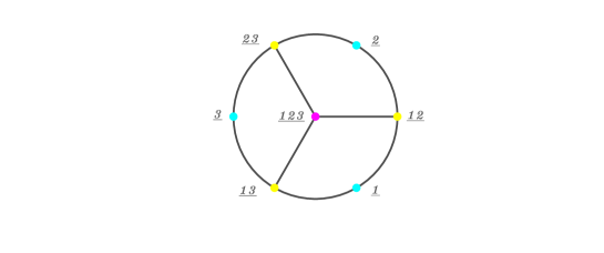
Figure 1. North Polar Cask for $d=3$.

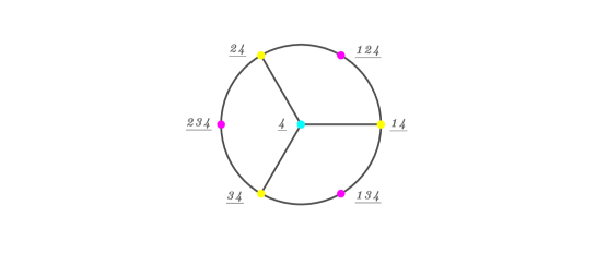
Figure 2. South Polar Cask for $d=3$.

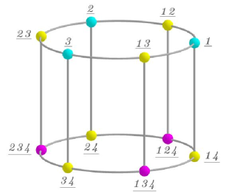
Figure 3. Ecuatorial Belt for $d=3$.

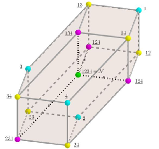
Figure 4. North Polar Cask for $d=4$.

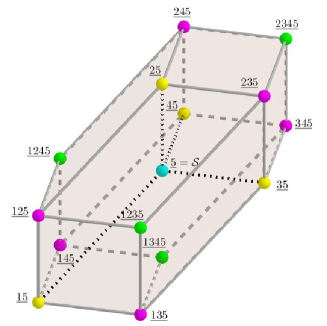
Figure 5. South Polar Cask for $d=4$.

5. Five conjectures proved for IAPs

Consider the set $\mathcal{M}$ of lower triangular infinite matrices with both entries and indices in $\mathbb{Z}_{\geq 0}$. Examples of matrices in $\mathcal{M}$ are the 2–power matrix, denoted $T$, defined by $T_{d,k}=\begin{cases}2^{d-k},&0\leq k\leq d,\\ 0,&\text{otherwise},\end{cases}$ and the Pascal matrix, denoted $P$, defined by $P_{d,k}=\begin{cases}{d\choose k},&0\leq k\leq d,\\ 0,&\text{otherwise.}\end{cases}$ With the Hadamard or entry–wise product, multiply the former matrices, obtaining $B:=T\circ P=P\circ T\in\mathcal{M}$ and notice that the $d$–th row of $B$ shows the $f$–vector of a $d$–box (padded with zeros), for $d\in\mathbb{Z}_{\geq 0}$; see (1.1). We call $B$ is the $f$–vector box matrix. Next, consider the matrix $H\in\mathcal{M}$ defined by

(5.1) $$H_{d,k}=\begin{cases}(2^{d-k}-1){{d+1}\choose k},&0\leq k\leq d-1,\\ 1/2,&k=d,\\ 0,&\text{otherwise.}\end{cases}$$

For fixed $d\geq 2$, we study the growth of the sequence $H_{d,k}$, with $0\leq k<k+1\leq d-1$.

Proposition 5.1.

For each $d\geq 0$, we have $H_{d,d-1}\leq H_{d,0}$ with equality only for $d=0,1,2$.

Proof.

The inequality $(d+1)d/2\leq 2^{d}-1$ is easily proved by induction on $d$ (degree 2 polynomials grow slower than 2–powers.) ∎

Recall that a sequence $a_{k}$ is log–concave if $a_{k+1}^{2}\geq a_{k}a_{k+2},\forall k$; see [7, 32].

Proposition 5.2.

For $d\geq 2$, the sequence $\{H_{d,k}:0\leq k\leq d-1\}$ is log–concave.

Proof.

For fixed $d$, the sequence $T_{d,k}-1=2^{d-k}-1$ is log–concave, because $(T_{d,k+1}-1)^{2}-(T_{d,k}-1)(T_{d,k+2}-1)=2^{d-k-2}>2>0$, for $0\leq k\leq d-3$. It is easy to check that any row of Pascal’s triangle is a log–concave sequence. Since the termwise product of two log–concave sequences (with the same number of terms) is log–concave, then the result follows for $H_{d,k}$. ∎

Notice $I_{d,k}=2H_{d,k}$, for $0\leq k{\leq}d$.

Corollary 5.3 (Unimodality holds for isocanted).

For each $d\geq 2$, the sequence $\{I_{d,k}:0\leq k\leq d-1\}$ is unimodal.

Proof.

It is easy to show that every log–concave sequence is unimodal (but not conversely). The sequence $H_{d,k}$ is unimodal and so is its double. ∎

Proposition 5.4.

For fixed $d\geq 2$, the maximum in the sequence $I_{d,k}$ is attained at the integer $\lfloor\frac{d}{3}\rfloor$.

Proof.

Cases $d=2$, 3 and 4 are checked directly (the $f$–vectors are $(6,6)$, $(14,24,12)$ and $(30,70,60,20)$). Assume $d\geq 5$ and $0\leq k\leq d-2$. Define the quotient

(5.2) $$Q_{d,k+1}:=\frac{I_{d,k+1}}{I_{d,k}}=\frac{(2^{d-k-1}-1)(d-k+1)}{(2^{d-k}-1)(k+1)}$$

and the terms

(5.3) $$L_{d,k+1}:=2^{d-k-1}(d-3k-1),\quad R_{d,k+1}:=d-2k.$$

We have $I_{d,k+1}\geq I_{d,k}$ if and only if $Q_{d,k+1}\geq 1$ if and only if $L_{d,k+1}\geq R_{d,k+1}$, because we have cleared the positive denominator in (5.2) and grouped terms. The exponent $d-k-1$ appearing in $L_{d,k+1}$ is at least 1. The sign of the factor $(d-3k-1)$ in $L_{d,k+1}$ is not constant. We have $\frac{d}{3}\leq\frac{2d-5}{3}$, since $d\geq 5$. We prove

1. if $k\leq\frac{d-2}{4}$, then $L_{d,k+1}\geq R_{d,k+1}$,

2. if $\frac{d-2}{4}\leq k\leq\frac{d-2}{3}$, then $L_{d,k+1}\geq R_{d,k+1}$,

3. if $\frac{d}{3}\leq k\leq\frac{2d-5}{3}$, then $L_{d,k+1}\leq R_{d,k+1}$,

4. if $\frac{2d-5}{3}\leq k$, then $L_{d,k+1}\leq R_{d,k+1}$,

and the result follows. Indeed,

1. the factor in $L_{d,k+1}$ is positive and so $L_{d,k+1}\geq 2(d-3k-1)\geq R_{d,k+1}$,

2. the factor in $L_{d,k+1}$ is at least 1, the exponent $d-k-1$ in $L_{d,k+1}$ is at least $\frac{d+2}{3}$ and $\frac{d+2}{2}\geq R_{d,k+1}$, so we have $L_{d,k+1}\geq 2^{\frac{d+2}{3}}(d-3k-1){\geq 2^{\frac{d+2}{3}}}\geq\frac{d+2}{2}\geq R_{d,k+1}$,

3. the factor in $L_{d,k+1}$ is no more than $-1$, the exponent $d-k-1$ in $L_{d,k+1}$ is at least $\frac{d+2}{3}$ and $R_{d,k+1}\geq\frac{-d+10}{3}$, so we get $R_{d,k+1}\geq\frac{-d+10}{3}\geq-2^{\frac{d+2}{3}}\geq 2^{\frac{d+2}{3}}(d-3k-1)\geq L_{d,k+1}$,

4. the factor in $L_{d,k+1}$ is non–positive and so $R_{d,k+1}\geq d-3k-1\geq L_{d,k+1}$.

It follows that the change in the monotonicity of the sequence $I_{d,k}$ occurs in the interval $\mathbb{Z}\cap[\frac{d-2}{3},\frac{d}{3}]$. For fixed $d\geq 2$, we have found the maximum in $I_{d,k}$ attained at $k=\lfloor\frac{d}{3}\rfloor=\begin{cases}\frac{d}{3},&d\equiv 0\mod 3,\\ \frac{d-1}{3},&d\equiv 1\mod 3,\\ \frac{d-2}{3},&d\equiv 2\mod 3.\end{cases}$ ∎

Corollary 5.5 (Bárány conjecture holds for isocanted).

If $d\geq{2}$ and $0\leq k<k+1\leq d-1$, then $I_{d,k}\geq\min\{I_{d,0},I_{d,d-1}\}=I_{d,d-1}=(d+1)d$.

Proof.

Use unimodality and Proposition 5.1. ∎

The $3^{d}$ conjecture and the flag conjecture were posed by Kalai in 1989, for centrally symmetric polytopes.

Corollary 5.6 ($3^{d}$ conjecture holds for isocanted).

For $d\geq 2$, it holds $\sum_{k=0}^{d}I_{d,k}=3^{d+1}-2^{d+2}+{2}$ and this is larger than $3^{d}$.

Proof.

The binomial theorem $(x+y)^{d}=\sum_{j=0}^{d}x^{j}y^{d-j}{d\choose j}$ with $x=1$ yields $2^{d}=\sum_{j=0}^{d}{d\choose j}$ and $3^{d}=\sum_{j=0}^{d}2^{d-j}{d\choose j}$. Then

(5.4) $$3^{d+1}-2\times 2^{d+1}=\sum_{j=0}^{d+1}2^{d+1-j}{{d+1}\choose j}-2\sum_{j=0}^{d+1}{{d+1}\choose j}=\sum_{j=0}^{d+1}(2^{d+1-j}-2){{d+1}\choose j}=\sum_{j=0}^{d-1}I_{d,j}+\text{two summands.}$$

Summand for $j=d$ is zero and for $j=d+1$ is ${-1}$, whence, using $I_{d,d}=1$, we get the claimed equality. Proof of the inequality: we have $2^{3}=8=3^{2}-1$ and $2^{d-2}<3^{d-2}$. Multiply termwise and get $2^{d+1}\leq 3^{d-2}(3^{2}-1)=3^{d}-3^{d-2}<3^{d}+1$ whence $2(2^{d+1}-1)<2\times 3^{d}=3^{d+1}-3^{d}$. ∎

Remark 5.7.

Recall that Stirling number of the second kind is the number of ways to partition $[d]$ into $k$ non–empty subsets, and it is denoted $S(d,k)$. We have $3^{d+1}-2^{d+2}+2=2S(d+2,3)+1$ (see Wikipedia and OEIS A101052, OEIS A028243 and OEIS A000392 in [31]).

Remark 5.8.

Recall that a Hanner polytope is obtained from closed intervals, by using two operations any finite number of times: Cartesian product and polar. They were studied by Hanner in 1956. Is $\mathcal{I}^{d}$ a Hanner polytope? Conversely, is some Hanner polytope an IAP? Since Hanner polytopes satisfy the $3^{d}$ conjecture and they attain the minimal conjectured value (see [28]), then the answer is NO in both cases.

Recall that a complete flag in a polytope $\mathcal{P}$ is a maximal chain of faces of $\mathcal{P}$ with increasing dimensions. Next, we count complete flags (and call them flags, for short). The number of flags in a $d$–box is $2^{d}d!$, because there are $2^{d}$ vertices and, at each one, there are $d!$ flags. The flag conjecture yields that boxes minimize flags among centrally symmetric polytopes; see [18, 28, 29].

Corollary 5.9 (Flag conjecture holds for isocanted).

The number of flags in $\mathcal{I}^{d}$ is $(d+1)(d-1)!(2^{d+1}-4)$ and it is larger than $2^{d}d!$, for $d\geq 2$.

Proof.

In $\mathcal{I}^{d}$ there are $2(d+1)$ vertices of valence $d$, and the remaining $2(2^{d}-d-2)$ vertices have valence $d+1$. Indeed, the vertices of length 1 or $d$ have valence $d$. A vertex of length $2\leq t\leq d-1$ has valence $d+1$, because it has $t$ parents and $d+1-t$ children. Reasoning as in boxes, we find $d!$ flags beginning at a vertex of valence $d$. Using Item 1 in Corollary 3.13, we find $(d+1)(d-1)!$ flags beginning at a vertex $V$ of valence $d+1$, because $\mathcal{I}^{d}$ is cubical and there are $d+1$ $(d-1)$–cuboids meeting at $V$. Thus, adding up, $2(d+1)\times d!+2(2^{d}-d-2)\times(d+1)(d-1)!=(d+1)(d-1)!(2^{d+1}-4)$ is the total number of flags. Further, we have $(2^{d-1}-1)(d+1)>2^{d-2}d$, for $d\geq 2$, whence the claimed inequality. ∎

The cubical lower bound conjecture (CLBC) was posed by Jockusch in 1993 and rephrased, in terms of the cubical $g$–vector $g^{c}$, by Adin et al. in 2019 as follows: is $g^{c}_{d,2}\geq 0$?; see [2, 17].

Proposition 5.10 (CLBC holds for isocanted).

$g^{c}_{d,2}\geq 0$ holds true for $\mathcal{I}^{d}$, for $d\geq 2$.

Proof.

We have computed the sequence $g^{c}_{d,2}$ for IAPs, obtaining $6,20,50,112,238,\ldots$; see OEIS A052515 in [31]. ∎

Recall that the distance between two vertices of a polytope is the minimum number of edges in a path joining them. The diameter of a polytope is the greatest distance between two vertices of the polytope.

Corollary 5.11 (Diameter of isocanted).

The diameter of $\mathcal{I}^{d}$ is $d+1$.

Proof.

Consider different proper subsets $W,W^{\prime}\subset[d+1]$ and assume $|W\cap W^{\prime}|=i$, $|W|=i+w$ ,$|W^{\prime}|=i+w^{\prime}$, with $i,w,w^{\prime}\geq 0$ and $i+w+w^{\prime}\leq d+1$. To go from vertex $\underline{W}$ to vertex $\underline{W^{\prime}}$ one must drop (one at a time) the $w$ digits in $W\setminus W^{\prime}$ and one must gain (one at a time) the $w^{\prime}$ digits in $W^{\prime}\setminus W$, whence $\operatorname{d}(\underline{W},\underline{W^{\prime}})=w+w^{\prime}$. In the particular case that $W^{\prime}$ is complementary to $W$, we get the greatest distance $\operatorname{d}(\underline{W},\underline{W^{\prime}})=d+1$. ∎

6. Future work

We would like to compute the $f$–vector of a general alcoved polytope.

Authors’ addresses: M.J. de la Puente, Universidad Complutense, Madrid, Spain, e-mail: mpuente@ucm.es. P.L. Clavería, Universidad de Zaragoza, Zaragoza, Spain, e-mail: plcv@unizar.es.

References

- [1] R.M. Adin: A new cubical h-vector, Proceedings of the 6th Conference on Formal Power Series and Algebraic Combinatorics (New Brunswick, NJ, 1994), 1996, 3 -14, MR1417283, Zbl 0861.52007, https://doi.org/10.1016/S0012-365X(96)83003-2
- [2] R.M. Adin, D. Kalmanovich and E. Nevo: On the cone of -vectors of cubical polytopes, Proc. Amer. Math. Soc. 147 (2019), 1851-1866, MR3937665, Zbl 07046511, DOI: https://doi.org/10.1090/proc/14380 Published electronically: January 18, 2019.
- [3] A. Barvinok: Integer points in polyhedra, Zurich Lectures in Advanced Mathematics, EMS, 2008, MR2455889, Zbl1154.52009.
- [4] T. Bisztriczky, P. McMullen, R. Schneider and I. Weiss (eds.): Polytopes: abstract, convex and computational, Kluwer Academic Pub., 1994, MR1322054, Zbl 0797.00016.
- [5] G. Blind and R. Blind: The cubical –polytopes with fewer than vertices, Discrete Comput. Geom. 13 (1995), no. 3-4, 321 345, MR 1318781, Zbl 0824.52013, https://doi.org/10.1007/BF02574048
- [6] G. Blind and R. Blind: The almost simple cubical polytopes, Discrete Math., 184, 25–48, (1998) DOI:10.1016/s0012-365x(97)00159-3, MR1609343, Zbl 0956.52008.
- [7] F. Brenti: Log–concave and unimodal sequences in algebra, combinatorics, and geometry: an update, Jerusalem combinatorics ’93, 71 89, Contemp. Math., 178, Amer. Math. Soc., Providence, RI, 1994, MR1310575, Zbl 0813.05007.
- [8] E. Brugallé: Un peu de géométrie tropicale, Quadrature, 74, (2009), 10–22, Zbl 1202.14055.
- [9] E. Brugallé: Some aspects of tropical geometry. Newsletter of the European Mathematical Society, 83, (2012), 23–28, MR2934649, Zbl 1285.14069.
- [10] P. Butkovič: Max–plus linear systems: theory and algorithms, Springer, 2010, MR2681232, Zbl 1202.15032 .
- [11] M. Develin and B. Sturmfels: Tropical convexity, Doc. Math. 9, 1–27, (2004) MR2054977 ; Erratum in Doc. Math. 9 (electronic), 205–206, (2004), MR2117413, Zbl 1054.52004.
- [12] M. Develin, F. Santos and B. Sturmfels: On the rank of a tropical matrix, in Discrete and Computational Geometry, E. Goodman, J. Pach and E. Welzl, eds., MSRI Publications, Cambridge Univ. Press, 2005, MR2178322, Zbl 1095.15001.
- [13] B. Grünbaum: Convex polytopes. With the cooperation of Victor Klee, M. A. Perles, and G. C. Shephard, , John Wyley and Sons, 1967, MR0226496, Zbl 0163.16603.
- [14] P. Guillon, Z. Izhakian, J. Mairesse and G. Merlet: The ultimate rank of tropical matrices, J. Algebra, 437, 222–248, 2015, MR3351964, Zbl 1316.15030.
- [15] M. Henk, J. Richter–Gebert and G.M. Ziegler: Basic properties of convex polytopes, Chapter 15 in Handbook of Discrete and Computational Geometry, J.E. Goodman, J. O’Rourke, and C.D. Tóth (editors), 3rd edition, CRC Press, Boca Raton, FL, 2017, MR1730169, Zbl 0911.52007.
- [16] A. Jiménez and M.J. de la Puente: Six combinatorial clases of maximal convex tropical polyhedra, prerint arXiv: 1205.4162v2, 2012.
- [17] W. Jockusch: The lower and upper bound problems for cubical polytopes, Discrete Comput. Geom. 9 (1993), no. 2, 159 163, MR1194033, Zbl 0771.52005, https://doi.org/10.1007/BF02189315
- [18] G. Kalai: The number of faces of centrally-symmetric polytopes, Graphs Comb. 5 (1989) 389–391, MR1554357, Zbl 1168.52303.
- [19] G. Kalai and M.G. Ziegler (eds.): Polytopes: combinatorics and computation, DMV Seminar 29, Birkhäuser, (2000), MR1785290, Zbl 0944.00089.
- [20] T. Lam and A. Postnikov: Alcoved polytopes I, Discrete Comput. Geom. 38 n.3, 453-478 (2007), MR2352704, Zbl 1134.52019.
- [21] G.L. Litvinov, V.P. Maslov, (eds.): Idempotent mathematics and mathematical physics, Proceedings Vienna 2003, American Mathematical Society, Contemp. Math. 377, (2005), MR2145152, Zbl 1069.00011.
- [22] G.L. Litvinov, S.N. Sergeev, (eds.): Tropical and idempotent mathematics, Proceedings Moscow 2007, American Mathematical Society, Contemp. Math. 495, (2009), MR2581510, Zbl 1172.00019.
- [23] G. Mikhalkin: What is a tropical curve?, Notices AMS, April 2007, 511–513, MR2305295, Zbl 1142.14300.
- [24] M.J. de la Puente: On tropical Kleene star matrices and alcoved polytopes, Kybernetika, 49, n.6, (2013) 897–910, MR3182647, Zbl 1297.15029.
- [25] M.J. de la Puente: Distances on the tropical line determined by two points, Kybernetika, 50, n.3, (2014) 408–335, MR3245538, Zbl 1321.14050.
- [26] M.J. de la Puente: Quasi–Euclidean classification of alcoved convex polyhedra, Linear Multilinear Algebra, 67 (2019), DOI 10.1080/03081087.2019.1572065.
- [27] J. Richter–Gebert, B. Sturmfels and T. Theobald: First steps in tropical geometry, in [21], 289–317, MR2149011, Zbl 1093.14080.
- [28] R. Sanyal, A. Werner and G.M. Ziegler: On Kalai s conjectures concerning centrally symmetric polytopes, Discrete Comput. Geom. (2009) 41, 183 -198, DOI 10.1007/s00454-008-9104-8, MR2471868, Zbl 1168.52013.
- [29] M. Senechal (ed.): Shaping Space: Exploring Polyhedra in Nature, Art, and the Geometrical Imagination, Springer, 2012, MR3087288, Zbl 1267.52002.
- [30] S. Sergeev: Multiorder, Kleene stars and cyclic projectors in the geometry of max cones, (2009) in [22], MR2581526, Zbl 1179.15033.
- [31] N.J. Sloane: The On–Line Encyclopedia of Integer Sequences, http://oeis.org/
- [32] R.P. Stanley: Log-concave and unimodal sequences in algebra, combinatorics and geometry, Graph theory and its applications: East and West (Jinan, 1986) Ann. New York Acad. Sci., vol. 576, New York Acad. Sci., New York, 1989, pp. 500 535, MR 1110850, Zbl 0792.05008.
- [33] M.W. Schmitt and G.M. Ziegler: Ten problems in geometry, in [29] (2012).
- [34] D. Speyer: Tropical linear spaces, SIAM J. Discrete Math. 22, no. 4, (2008) 1527 -1558, MR2448909, Zbl 1191.14076.
- [35] D. Speyer, B. Sturmfels: The tropical Grassmannian, Adv. Geom. 4, 389–411, (2004), MR2071813, Zbl 1065.14071.
- [36] N.M. Tran: Enumerating polytropes, J. Combin. Theory Ser. A, 151, (2017) 1–22, MR3663485, Zbl 06744864.
- [37] A. Werner and J. Yu: Symmetric alcoved polytopes, The Electronic Journal of Combinatorics 21 (1) (2014), Paper 1.20, 14 pp, arXiv: 1201.4378v1 (2012), MR3177515, Zbl 1302.52014.
- [38] B. Yu, X. Zhao and L. Zeng: A congruence on the semiring of normal tropical matrices, Linear Alg. Appl. 555, (2018), 321–335, https://doi.org/10.1016/j.laa.2018.06.027, MR3834207, Zbl 1396.15022.
- [39] G.M. Ziegler: Lectures on polytopes, GTM 152, Springer, 1995, MR1311028, Zbl 0823.52002.
- [40] G.M. Ziegler: Convex polytopes: extremal constructions and –vector shapes, IAS Park City Math. Series, 14, 2004, MR2383133, Zbl 1134.52018.