Distributed learning for optimal allocation of synchronous and converter-based generation

Abstract

Motivated by the penetration of converter-based generation into the electrical grid, we revisit the classical log-linear learning algorithm for optimal allocation of synchronous machines and converters for mixed power generation. The objective is to assign to each generator unit a type (either synchronous machine or DC/AC converter in closed-loop with droop control), while minimizing the steady state angle deviation relative to an optimum induced by unknown optimal configuration of synchronous and DC/AC converter-based generation. Additionally, we study the robustness of the learning algorithm against a uniform drop in the line susceptances and with respect to a well-defined feasibility region describing admissible power deviations. We show guaranteed probabilistic convergence to maximizers of the perturbed potential function with feasible power flows and demonstrate our theoretical findings via simulative examples of power network with six generation units.

I INTRODUCTION

With increased share of renewable energy resources (wind, solar, fuel cells, etc.) in the electrical grid, it is of uttermost importance to understand the ramification of penetration of converter-based generation on the operation and maintenance of normal grid conditions. Since a large percentage of power system generation will withdraw synchronous machines and replace these gradually by power converters [1]. This motivates the ongoing efforts to optimize the grid performance in mixed power generation, i.e., in the presence of synchronous machines and converters using tools from optimization theory [2].

In particular, the field of game theory has gained more and more attention over the years as it intersects several disciplines. Game theory offers a rich set of model elements, solution concepts, and evolutionary notions. Within the realm of engineering systems, a key element in the use of game theory is to design incentives to obtain desirable behaviors [3, 4]. A game theoretical model is more than just a dynamic feedback system, as each player learns the environment, which in turn learns the player [4].

Different game theoretic concepts have been previously applied to formulate and solve optimization problems in power systems. For example, in [5] a feedback controller is proposed based on population games to achieve frequency regulation and economic efficiency. The authors of [6, 7] design distributed control laws for decision process of individual sources in small-scale DC power systems and propose a proportional allocation mechanism using non-cooperative game theory, respectively. In [8], coalitional game approach allows consumers to cooperatively share storage with each other, while minimizing electricity consumption cost. Moreover, game theory has been leveraged for pricing and market mechanisms in power systems [9, 10, 11] as well as security assessment and mitigation of attacks [12, 13].

Learning in game theory provides a framework for designing, analyzing and controlling multi-agent systems [14] and is well-understood in the literature with guaranteed asymptotic results, for example, convergence to a Nash equilibrium. Learning algorithms have been extensively studied in potential games [15, 16] and are designed with the goal to implement a prescriptive control approach, where the guaranteed limiting behavior represents a desirable operating condition [17]. In particular, log-linear learning originally introduced in [18] is a learning algorithm that ensures that the action profiles that maximize the global objective of the multi-agent system coincide with the potential function maximizers. The inclusion of the noise function enables the players to occasionally make mistakes corresponding to sub-optimal actions. As the noise vanishes, the probability that a player selects a best response or an optimal action goes to one [17].

In this work, our contributions are put together as follows: First, we consider the log-linear learning algorithm in its classical formulation [18] through new lenses by applying it to an optimal allocation of synchronous and converter-based generation for radial power systems, where the goal is to assign a type (DC/AC converter in closed-loop with droop control or synchronous machine) to each generation unit, by minimizing steady state angle deviations with respect to an optimum. Our study aims to understand the ramifications of the penetration of converter-based generation on the construction of future microgrids, where synchronous machines are gradually withdrawn and replaced by DC/AC converters with suitable control [19]. Our analysis helps for e.g., making the decision on which synchronous machines to withdraw in the electrical grid, while gradually replacing these with converters at different penetration levels [20]. Second, we investigate the robustness of the learning algorithm against uniform drop in the line susceptances, representing uncertainty in the knowledge of their exact value, while steady state power deviations are confined to well-defined feasibility region. This is performed by determining an upper bound on the allowed line susceptance drop. Additionally, we show that the learning algorithm for optimal allocation of generation units converges, in the probabilistic sense, to an optimal configuration that corresponds to minimizers of the perturbed potential function representing the overall cost function of the potential game. Third, we validate our findings on a power system setup consisting of six generation units arranged according to a line graph. We simulate the power system with unperturbed as well as perturbed weight susceptances and discuss the convergence to an unknown optimal configuration for a susceptance perturbation within the derived theoretical bound.

The remainder of this paper unfurls as follows. Section II introduces the power systems model, as well as game-theoretic setup and formulates optimal allocation problem for radial power systems. In Section III, we study the robustness of the learning algorithm with respect to uniform drop in the line susceptances, provide interpretation to our results and link these to other well-studied optimization problems. Finally, Section IV illustrates our results by providing numerical simulations of the learning algorithm for optimal allocation on a network consisting of aligned six- generation units.

II Learning for optimal allocation in power systems

II-A Modeling of power systems

We consider a power network model, defined by a graph ${G}=(\mathcal{V},\mathcal{E})$ in radial (or acyclic) undirected network (see [21, 22]), where $\mathcal{V}$ is the set of $n$ (possibly) heterogeneous generation units, i.e., synchronous and converter-based generation. These can also be encountered for example in generation networks undergoing construction, where synchronous machines are gradually withdrawn or microgrids, where the converters have heterogeneous control parameters. Let $\mathcal{E}$ be the set of $m$ edges (purely inductive transmission lines) with susceptance weight $b_{e}>0,\,e\in\mathcal{E}$. The voltage magnitude $V_{i}$ at the $i$-th bus is assumed to be constant and equal to 1 per unit. We consider inductive loads with constant susceptances, absorbed in the lines. Define $\{1,\dots,n\}$ as the index set of all the generation units in the power system.

We denote by $\mathcal{I}\in{}^{n\times m}$ the incidence matrix of the graph ${G}$ and by $\mathcal{N}_{i}$ the neighbor set of the $i$-th generation unit (synchronous machine [23], or DC/AC converter in closed-loop with the droop control [22]). Under the assumption of quasi-stationary steady state, the swing equation of the $i$-th synchronous machine with known inertial constant $m_{i}>0$ and damping coefficient $d_{i}>0$ describes the $i$-th generation unit dynamics as follows,

$$m_{i}\ddot{\theta}_{i}(t) =-d_{i}\dot{\theta}_{i}(t)-\sum_{j\in\mathcal{N}_{i}}\,b_{ij}\sin(\theta_{i}(t)-\theta_{j}(t))+P_{0,i},$$ (1)

where $\theta_{i}(t)\in\real$ denotes the (virtual) voltage phase angle, $P_{0,i}\in\real$ is a constant power input that represents mechanical or DC side power input and $P_{i}=\sum_{j\in\mathcal{N}_{i}}b_{ij}\sin(\theta_{i}(t)-\theta_{j}(t))$ is the electrical power injected from the $i$-th generation into the neighbor set $\mathcal{N}_{i}$. The dynamics in (1) describes both DC/AC converters that are equipped with droop control, or the rotor dynamics of synchronous machines, where the difference between the two models lies in the parameter values of the damping $d_{i}$ and inertia $m_{i}$.

In the sequel, we denote the phase angles of the generation units at steady state by $\theta^{s}=\begin{bmatrix}\theta_{1}^{s},\dots,\theta_{n}^{s}\end{bmatrix}^{\top}$, induced by configuration (or arrangement) of the generation units $s=[s_{1},\dots,s_{n}]^{\top}$, where $s_{i}\in\mathcal{S}=\{M,C\}$ is the type (synchronous machine (M), or DC/AC converter (C)) of the $i$-th generation unit. The steady state angles are described by the following equation,

$$d_{i}\dot{\theta}_{i}^{s}=-\sum_{j\in\mathcal{N}_{i}}b_{ij}\sin(\theta^{s}_{ij})+P_{0,i},\;\theta^{s}_{ij}=\theta^{s}_{i}-\theta^{s}_{j}.$$ (2)

After defining the steady state power vector $P_{0}=\begin{bmatrix}P_{0,1},\dots,P_{0,n}\end{bmatrix}^{\top}$, the damping matrix $D=\text{diag}\{d_{i}\}_{i=1\dots n}$, as well as $\mathds{1}_{n}$ the vector of all ones, we make the following assumption.

Assumption 1 (Flow feasibility [22]).

Consider the power system model at steady state in (2). We assume that

$$||\mathrm{diag}(\{b_{ij}\}_{(i,j)\in\mathcal{E}})^{-1}\cdot\xi^{s}||_{\infty}<1,$$ (3)

for all configurations $s$, where $\xi^{s}\in{}^{m}$ is the vector of edge flows satisfying,

$$P_{0}-\omega_{0}\,D\,\mathds{1}_{n}=\mathcal{I}\,\xi^{s},$$ (4)

with $\omega_{0}=\sum_{i=1}^{n}P_{0,i}/\sum_{i=1}^{n}d_{i}$, and $\lVert\cdot\rVert_{\infty}$ denotes the supremum norm.

For a given configuration $s=[s_{1},\dots,s_{n}]^{\top}$ and damping matrix $D$, the steady state angle differences $\theta_{ij}^{s}$ are determined from,

$$\underline{\sin}(\mathcal{I}^{\top}\theta^{s})=\text{diag}(\{b_{ij}\}_{(i,j)\in\mathcal{E}})^{-1}\xi^{s},$$ (5)

with $\underline{\sin}(z)=[\sin(z_{1}),\dots,\sin(z_{m})]^{\top}$ and the edge flow vector $\xi^{s}$ is defined in (4).

It is important to mention that, the damping parameter of synchronous machines is considered to have higher value, than that of DC/AC converters in closed loop with droop control and enters the power balance equation (4) through the damping matrix $D$. The values of the damping coefficients are obtained from the design characteristics of synchronous machines or converters at hand and can be tuned via torque control for machines or proportional control on the DC side for converters. This establishes the link between a configuration $s=[s_{1},\dots,s_{n}]$ and the corresponding relative steady state angles $\theta^{s}_{ij}$. Physically, the parametric condition (3) in Assumption 1 states that the active power flow along each edge be feasible, i.e., less than the physical maximum. It is equivalent to the existence of unique and synchronized steady state angles $\theta^{s}=[\theta_{1}^{s},\dots,\theta_{n}^{s}]^{\top}$, that are phase cohesive, i.e., $\theta^{s}_{ij}<\gamma,\gamma\in[0,\pi/2[$ for all $i,j\in\mathcal{V}$ satisfying (5). For more details about the derivation of (4) and (5), we refer the interested reader to Theorem 2 in [22].

Let $\theta_{ij}^{s^{*}},(i,j)\in\mathcal{E}$ denote known optimal phase angle differences corresponding to an optimal, yet unknown configuration $[s^{\text{*}}_{1},\dots,s^{\text{*}}_{n}],\,s^{*}_{i}\in\mathcal{S}=\{M,C\}$. These can be obtained, for example, from historical records of the optimal power system operation of other microgrids or power generation under similar setups.

II-B Game-theoretic setup

Consider a game $(\mathcal{V},\mathcal{A},\{u_{i}\}_{i\in\mathcal{V}})$, where $\mathcal{V}$ is a finite set of players and $\mathcal{A}$ is a set of actions. Each player $i\in\{1,\dots,n\}$ has a utility function $u_{i}$ (a.k.a reward or payoff function), which associates with every action $x\in\mathcal{X}=\mathcal{A}^{\mathcal{V}}$ the utility $u_{i}(x)$ that player $i$ gets, when every other player $j\in\mathcal{N}_{i}$ is playing action $x_{j}\in\mathcal{A}$. Let $x_{-i}=(x_{1},x_{2},\dots,x_{i-1},x_{i+1},\dots,x_{n})$ denote the profile of all players’ actions, other than player $i$.

Definition II.1 (Potential game, [3]).

A game $(\mathcal{V},\mathcal{A},\{u_{i}\}_{i\in\mathcal{V}})$ is called a potential game, if there exists a function $U:\mathcal{X}\to\real$ (referred to as the potential function of the game), such that for any two configurations $x,y\in\mathcal{X}$ and a player $i\in\mathcal{V}$, we have that,

$$u_{i}(y_{i},x_{-i})-u_{i}(x_{i},x_{-i})=U(y_{i},x_{-i})-U(x_{i},x_{-i}).$$

A potential game as defined above requires perfect alignment between the global objective and the players’ local objective functions, so that the change in a player’s utility that results from a unilateral change in strategy equals the change in the global utility [3].

Definition II.2 (Pure strategy Nash equilibrium).

A (pure strategy) Nash equilibrium for the game $(\mathcal{V},\mathcal{A},\{u_{i}\}_{i\in\mathcal{V}})$ is an action configuration $x^{*}\in\mathcal{X}$, such that,

$$x^{*}_{i}\in\mathcal{B}_{i}(x^{*}_{-i}),\,i\in\mathcal{V},$$

where $\mathcal{B}_{i}(x_{-i})=\text{argmax}_{x_{i}\in\mathcal{A}}u_{i}(x_{i},x_{-i})$ is the best response function.

A pure Nash equilibrium as given in Definition II.2, represents a configuration, in which no player has a unilateral incentive to deviate from his current action.

Definition II.3 (Noisy best response).

Consider a game $(\mathcal{V},\mathcal{A},\{u_{i}\}_{i\in\mathcal{V}})$. The continuous-time asynchronous noisy best response dynamics is a Markov chain $X(t)$ with state space $\mathcal{X}=\mathcal{A}^{\mathcal{V}}$, where each player is equipped with an independent rate-1 Poisson clock. If the clock ticks at time $t$, the player $i$ updates his actions to $s$, chosen from a conditional probability:

$$P(X_{i}(t+1)=s|\,X_{i}(t))=\frac{e^{1/\tau(t)\cdot u_{i}(s,X_{-i})}}{\sum\limits_{X_{i}\in\mathcal{A}_{i}}e^{1/\tau(t)\cdot u_{i}(X_{i},X_{-i})}},$$ (6)

where $\tau(t)>0$ is the temperature or noise function that controls the smoothness of (6) and is a decreasing function of time [17].

Note that $\tau(t)$ determines how likely is player $i$ to select a sub-optimal action: As $\tau(t)\to\infty$, player $i$ will select any unit type $X_{i}$ with equal probability. As $\tau(t)\to 0$, the only stochastically stable states (see Definition 4, in [24]) of the Markov process are the joint actions that maximize the potential function. This shows the probabilistic convergence of the log-linear learning algorithm, and hence that of the learning algorithm for optimal allocation, to a Nash equilibrium that maximizes the potential function [25, 17].

The algorithm described in Definition II.3 is known as log-linear algorithm, and is well studied in game theory and classically described by the following rules [17]:

• Players’ utility functions constitute a potential game.

• Players update their strategies one at a time, which is referred to as asynchrony.

• At any stage, a player can select any action in the action set.

• Each player assesses the utility for alternative actions, assuming that the actions of all other players remain fixed.

II-C Optimal allocation problem

In this section, our goal is to assign a type $s_{i}\in\mathcal{S}=\{M,C\}$ to each generation unit $i\in\{1\dots n\}$, represented by a Markov chain $X(t)=[X_{1}(t),\dots,X_{n}(t)]^{\top}$ with $X_{i}(t)=s_{i}\in\mathcal{S}$ being the generation unit type of player $i$ at time $t$. This assignment is performed so that, the phase angles at each unit are the closest to their given optimal relative angles $\theta_{ij}^{s^{*}}$, derived from an unknown optimal configuration $s^{*}$ of the converters and synchronous machines. In other words, we aim to find a valid generation unit assignment $s=[s_{1},\dots,s_{n}]^{\top}$ by finding $X=[X_{1},\dots X_{n}]^{\top}$, so as to minimize the pairwise interaction cost,

$$c\,(X_{i}(t)=s_{i},\,X_{j}(t))=|\sin(\theta^{s}_{i{j}})-\sin(\theta^{s^{*}}_{ij})|,$$ (7)

where $\theta^{s}_{ij}=\theta^{s}_{i}-\theta^{s}_{j}$ and $\theta^{s^{*}}_{ij}=\theta^{s^{*}}_{i}-\theta^{s^{*}}_{j}$ are steady state angle relative differences, resulting from choosing the type $s_{i}$ for the $i$-th generation unit, given the generation types of the neighboring units $s_{j},j\neq i$.

The interaction cost in (7) depends implicitly on the configuration $X=s,\,s_{i}\in\mathcal{S},\,i=1\dots n$, through (4) and (5).

At every time instance $t$, one generation unit $g(t)\in\{1\dots n\}$ chosen uniformly at random wakes up and updates its type $s_{i}\in\mathcal{S}$. The conditional probability of updating the $i$-th generation unit to type $s_{i}$ is given by,

$$P(X_{i}(t+1) =s_{i}\;|\;X(t),\,g(t)=i)$$ (8)

$$=\!\frac{\!\!e^{-1/\tau(t)\sum_{j\in\mathcal{N}_{i}}b_{ij}\,c\,(s_{i},X_{j}(t))}}{\!\!\sum\limits_{k\in\mathcal{S}}e^{-1/\tau(t)\sum_{j\in\mathcal{N}_{i}}b_{ij}\,c\,(k,X_{j}(t))}},$$

where the temperature function $\tau(t)$ is defined as in (6).

We assign to each player an objective function that captures the player’s marginal contribution to the potential function. This translates to assigning to each player the following utility function,

$$u_{i}(X_{i},X_{-i})=-\sum\limits_{j\in\mathcal{N}_{i}}b_{ij}\,c\,(X_{i},X_{j}).$$ (9)

Next, we define the potential function given by,

$$U(X)=-\frac{1}{2}\sum\limits_{\begin{subarray}{c}i,j\in\mathcal{V},\\ (i,j)\in\mathcal{E}\end{subarray}}b_{ij}\,c\,(X_{i}(t),X_{j}(t)).$$ (10)

Following Assumption 1, the aforementioned potential function (10) achieves zero if and only if all generation units are aligned with an optimal configuration $s^{*}=[s_{1}^{*},\dots,s_{n}^{*}]^{\top}$ of converters and synchronous machines. This can be seen from,

$$|\sin(\theta^{s}_{i{j}})-\sin(\theta^{s^{*}}_{ij})|=0,$$

if and only if $\theta^{s}_{ij}=\theta^{s^{*}}_{ij}$, for all $i=1,\dots,n$. In fact, given optimal steady state angle $\theta^{s^{*}}$, we can write (4) as

$$D^{*}\,\mathds{1}_{n}=\frac{1}{\omega_{0}}\left[P_{0}-\mathcal{I}\,\text{diag}(\{b_{ij}\})\sin(\mathcal{I}^{\top}\theta^{s^{*}})\right]$$

and thus deduce from the optimal arrangement of damping coefficients $D^{*}\,\mathds{1}_{n}=[d^{*}_{1},\dots,d^{*}_{n}]^{\top}$, the corresponding optimal configuration $s^{*}$.

Note that an optimal configuration $s^{*}=[s_{1}^{*},\dots s_{n}^{*}]^{\top}$ is a Nash equilibrium of the game, given by the utility function (9), because it maximizes the potential function (10). However, a Nash equilibrium $X^{*}=[X^{*}_{1},\dots,X^{*}_{n}]^{\top}$ can be sub-optimal, i.e., $U(X^{*})<0$, and hence may fail to correspond to an optimal configuration and thus may not be a maximizer of the potential function (10).

III Robustness of optimal allocation problem

III-A Drop in transmission line susceptances

In this section, we investigate the implication of an additive unknown perturbation in transmission line susceptances on the probabilistic convergence of the log-linear algorithm and its robustness with respect to a well-defined feasibility region of admissible power flows.

Under these settings, we define the utility function for the $i$-th generation unit as follows,

$$\hat{u}_{i}(X)=-\sum\limits_{j\in\mathcal{N}_{i}}\hat{b}_{ij}(\delta)\,c(X_{i}(t),X_{j}(t)),$$ (11)

where $\hat{b}_{ij}(\delta)=b_{ij}-\delta,\,0\leq\delta<b_{ij}$, as well as the perturbed potential function,

$$\hat{U}(X)=-\frac{1}{2}\sum\limits_{\begin{subarray}{c}i,j\in\mathcal{V},\\ (i,j)\in\mathcal{E}\end{subarray}}\hat{b}_{ij}(\delta)\,c\,(X_{i}(t),X_{j}(t)).$$ (12)

Hence, $\delta$ represents a uniform drop in the line susceptances so that the perturbed weights are still positive [26]. A drop in the susceptance value models commonly encountered uncertainty in the knowledge about the exact values of line parameters in power systems [27, 28].

In the sequel, we assume that Assumption 1 holds with perturbed weights, for all $0\leq\delta<b_{ij},\,(i,j)\in\mathcal{E}$ and configurations $s$., i.e.,

$$\lVert\text{diag}(\hat{b}_{ij}(\delta))^{-1}\xi^{s}\rVert_{\infty}<1,$$ (13)

where $\xi^{s}$ represent edge flow vector that solves the power balance equations (5) with the perturbed weights $\hat{b}_{ij}>0$.

Let $\theta_{ij}^{s}$ denote the relative steady state angles resulting from solving for the power balance equations (4), (5) with the perturbed line susceptances $\hat{b}_{ij}$, for all $i,j\in\mathcal{V}$. Next, we introduce a set of steady state angles $\theta^{s}$, characterizing a feasibility region described by the maximal steady state power injected by each of the converters, relative to their optimal power output, i.e., corresponding to an optimal configuration $s^{*}$ of the unperturbed susceptances $b_{ij}$ as follows,

$$\mathcal{P}^{\alpha}(\theta^{s})=\left\{\theta^{s}\in{}^{n},\right.$$ (14)

$$\left.\max\limits_{i=1\dots n}|\sum\limits_{j\in\mathcal{N}_{i}}\hat{b}_{ij}(\delta)\sin(\theta^{s}_{ij})-\sum\limits_{j\in\mathcal{N}_{i}}b_{ij}\sin(\theta_{ij}^{s^{*}})|<\alpha\right\},$$

where $\sum_{j\in\mathcal{N}_{i}}\sin(\theta_{ij}^{s})>0$ for all $s$ (by phase angle cohesiveness of $\theta_{ij}^{s}$). We choose $\alpha>0$, so that, $\max\limits_{i=1\dots n}\left|\sum\limits_{j\in\mathcal{N}_{i}}b_{ij}\left(\sin(\theta_{ij}^{s})-\sin(\theta_{ij}^{s{{}^{*}}})\right)\right|<\alpha$, for all $s$. Thus, for the unperturbed susceptances ($\delta=0$), the steady state angles pertain to the feasibility region (14). In fact, for all feasible power flows (satisfying Assumption 1) the region $\mathcal{P}^{\alpha}$ in (14) can also be expressed in terms of the edge flows as $\{\xi^{s}\in{}^{m},\,||\mathcal{I}(\xi^{s}-\xi^{s^{*}})||_{\infty}<\alpha\}$.

Definition III.1.

The optimal allocation robustness margin is defined by,

$$\overline{R}^{s}=\inf\{\delta,\;\theta^{s}\not\in\mathcal{P}^{\alpha}(\theta^{s})\}.$$ (15)

This definition implies that the robustness margin is defined by the smallest susceptance drop $\delta$, that steers the steady state angles $\theta^{s}$, outside of their feasiblity region $\mathcal{P}^{\alpha}$. At this stage, we ask two fundamental questions:

• For $\tau(t)\to 0$, does the distributed learning algorithm for optimal allocation by means of the perturbed utility function (11), converge in probability towards maximizers of the perturbed potential function (12)?

• Can we identify the robustness margin $\overline{R}^{s}$ and determine its dependence on network parameters/configuration?

We provide answers to these questions in the following theorem.

Theorem III.2.

Let $\alpha>0$ be given as in (14). Consider the power system at steady state (2) with perturbed weights $\hat{b}_{ij}=b_{ij}-\delta$ and the utility function (11). Assume that (13) holds and define,

$$\overline{R}^{s} =\min_{i=1,\dots,n}\frac{\alpha+\sum\limits_{j\in\mathcal{N}_{i}}\left(b_{ij}(\sin(\theta^{s}_{ij})-\sin(\theta^{s^{*}}_{ij}))\right)}{\sum\limits_{j\in\mathcal{N}_{i}}\sin(\theta_{ij}^{s})}.$$ (16)

Additionally, consider the interaction cost (7) with optimal relative angles, corresponding to unknown configuration of the power system with perturbed weights $\hat{b}_{ij}$. Then, the following holds:

1. The distributed learning algorithm converges as $\tau(t)\to 0$, to the uniform probability over the set of best responses, which are maximizers of the perturbed potential function (12).

2. For every configuration $s$, the power system model is robust against uniform perturbations in the susceptances with a robustness margin given by $\overline{R}^{s}$ in (16), if and only if $\delta<\overline{R}^{s}$.

Proof.

Consider the cost function (7) with optimal steady state angles, that solve (4) and (5) with the perturbed weights $\hat{b}_{ij}=b_{ij}-\delta$. To prove the first statement, we follow the same lines of the proof of Proposition 3.1 from [17]. For this, we adopt the proof of Lemma 3.1 to our setup as follows: The perturbed learning algorithm for optimal allocation induces a finite, irreducible, aperiodic process over the state space. By introducing $\epsilon=e^{-1/\tau}$, we denote by $P^{\epsilon}$ the corresponding transition matrix.

By using the perturbed utility function in (11), we have

$$\lim_{\epsilon\to 0}\frac{P_{X\to X^{\prime}}^{\epsilon}}{\epsilon^{\max_{X_{i}}u_{i}(X)-\hat{u}_{i}(X^{\prime})}} =\frac{1}{n}\frac{1}{\sum\limits_{X_{i}\in\mathcal{A}_{i}}\epsilon^{\max_{X_{i}}u_{i}(X)-\hat{u}_{i}(X)}}<\infty,$$ (17)

with $X=(X_{i},X_{-i}),\,X^{\prime}=(X^{\prime}_{i},X_{-i})$, if and only if, $\max\limits_{X_{i}}u_{i}(X)-\hat{u}_{i}(X)\geq 0$. This means that, for all $X_{i}\notin\mathcal{B}_{i}(X_{-i})$, we have

$$\frac{u_{i}(X)-\max\limits_{X_{i}}u_{i}(X)}{\sum\limits_{j\in\mathcal{N}_{i}}c(X_{i},X_{j})}<\delta,$$ (18)

and taking the maximum, yields the lower bound,

$$\underline{R}^{s}=\max_{i=1,\dots,n}\frac{u_{i}(X)-\max\limits_{X_{i}}u_{i}(X)}{\sum\limits_{j\in\mathcal{N}_{i}}c_{i}(X_{i},X_{j})}<0.$$ (19)

Since $0\leq\delta$, this shows that $\underline{R}^{s}<\delta$. Hence, Lemma 3.1 holds with the resistance $r(X\to X^{{}^{\prime}})=\max_{X_{i}}u_{i}(X)-\hat{u}_{i}(X^{\prime})$. Together with Lemma 3.2, Proposition 3.1 in [17] implies that stochastically stable states are the set of perturbed potential function maximizers given in (12) .

To prove the second claim, we note that $\theta^{s}\notin\mathcal{P}^{\alpha}$ in (14), if and only if,

$$|\sum_{j\in\mathcal{N}_{i}}\hat{b}_{ij}(\delta)\sin(\theta^{s}_{ij})-\sum_{j\in\mathcal{N}_{i}}b_{ij}\sin(\theta^{\text{s}^{*}}_{ij})|\geq\alpha,$$

for some $i=1\dots n$. From $\hat{b}_{ij}=b_{ij}-\delta$, we solve for $\delta$, the resulting inequality,

$$|\sum_{j\in\mathcal{N}_{i}}b_{ij}(\sin(\theta^{s}_{ij})-\sin(\theta^{\text{s}^{*}}_{ij}))-\delta\sum_{j\in\mathcal{N}_{i}}\sin(\theta^{s}_{ij})|\geq\alpha.$$

This shows that,

$$\delta\geq\frac{\alpha+\sum\limits_{j\in\mathcal{N}_{i}}\left[b_{ij}(\sin(\theta^{s}_{ij})-\sin(\theta^{s^{*}}_{ij}))\right]}{\sum\limits_{j\in\mathcal{N}_{i}}\sin(\theta_{ij}^{s})},$$

or

$$\delta\leq\frac{-\alpha+\sum\limits_{j\in\mathcal{N}_{i}}\left[b_{ij}(\sin(\theta^{s}_{ij})-\sin(\theta^{s^{*}}_{ij}))\right]}{\sum\limits_{j\in\mathcal{N}_{i}}\sin(\theta_{ij}^{s})}.$$

By choice of $\alpha$ and definition of the robustness margin in (15), only the first inequality holds and we find the upper bound in (16) with $\overline{R}^{s}>0$. ∎

III-B Discussion

1. Theorem 1 establishes a robustness margin $\overline{R}^{s}$ with respect to a uniform drop in the line susceptance. The robustness margin $\overline{R}^{s}$ depends on the configuration $s$ and on admissible maximal deviation of steady state electrical power from its optimal value $\alpha$ described in (14). Note that, optimal steady state angles of the power system with perturbed susceptances are in general unknown. In this case, the learning algorithm with perturbed susceptances does not converge to a maximizer of $\hat{U}(t)$. See later Section IV.

2. A suitable choice of the temperature or noise function $\tau(t)$, as a decreasing function of time, is crucial for the improvement of the algorithm convergence properties. The function $\tau(t)$ determines the exploration rate of the learning algorithm [24].

3. The convergence in unperturbed (see Section II-B) as well as perturbed case (in Theorem III.2) is understood only in a probabilistic sense, that is, a Markov chain $X(t)$ itself can converge to a Nash equilibrium that is not a maximizer of the potential function $U(X)$. Hence, the potential function $U(X)$ is not always necessarily zero at the end of the learning algorithm.

4. The optimal allocation of synchronous and converter-based generation can be regarded in a broader perspective as a resource allocation problem [3], where the cost function (9) represents the welfare function. This can also be formulated as a task assignment [29, 30] for dynamic multi-agent networks, where each node selects its task, i.e., type from an admissible set and the cost function is interpreted as utility of an assignment profile for each node with a specific role.

IV Simulations

To illustrate the distributed learning for optimal allocation of synchronous and converter-based generation, we study an example of power systems represented by a line graph of six generation units and associated with power input vector (in p.u.) $P_{0}=[0.77778,0.7,0.798889,0.7,0.798889,0.7]^{\top}$. The susceptances $\{b_{ij}\}_{(i,j)\in\mathcal{E}}$ are given (in p.u.) by the matrix $\Gamma=\text{diag}\left\{[15.2631,4.2350,4.8156,15.2631,4.2350]\right\}$. The values are taken from the IEEE 14-bus system [31].

The goal is to assign a generation type $s_{i}\in\mathcal{S}$ to each generation unit $i\in\{1,\dots,6\}$. The optimal yet unknown configuration $s^{*}$, shown in Figure 1, is given by optimal steady state angles, which are minimizers of the potential function $U(t)$ in (10). The optimal relative angle differences $\{\theta^{s^{*}}_{ij}\}_{i,j\in\mathcal{V}}$ are given by $[-0.0157,-0.0354,0.0081,{0.0084},0.0750]^{\top}$. The distributed learning algorithm for optimal allocation aims to correctly assign a type (synchronous machine or DC/AC converter in closed-loop with droop control) and thus decide on which synchronous machine to withdraw and replace with DC/AC converter. The optimal configuration $s^{*}$, based on the given optimal angle differences $\{\theta^{s^{*}}_{ij}\}_{i,j\in\mathcal{V}}$.

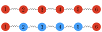
Figure 1: Top: Power system represented by a line graph consisting of six synchronous machines connected via inductive lines with susceptances $b_{ij}>~{}0$. Bottom: Unknown optimal configuration $s^{*}=[{M,C,C,C,C,M}]^{\top}$ corresponding to given optimal relative angles $\{\theta^{*}_{ij}\}_{i,j\in\mathcal{V}}$. The color red refers to a synchronous machine and blue to DC/AC converters (in closed-loop with droop control).

For this, we choose between two colors: red for synchronous machines $(M)$ and blue for DC/AC converters $(C)$ with respective damping values (in p.u.) $d_{C}=15$ and $d_{M}=25$. At initialization, all generation units are assumed to be synchronous machines, so that $X_{i}(t)=M,i=1,\dots,n$. We begin with the unperturbed ($\delta=0$) cost function (9). At each time $t>0$, a generation unit $i\in U(t)$ is chosen uniformly (at random) and updates its generation type $s_{i}$ (and hence color), according to the conditional probability (8). In Figure 2, we plot the time evolution of the potential function in (10), for two different realizations of the inverse of the temperature function $\eta(t)=1/\tau(t)$. Note that an increase in the slope of $\eta(t)$ is accompanied by an increase in the convergence rate to an optimal configuration.

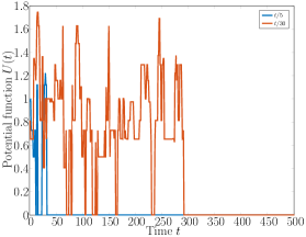
Figure 2: Evolution of the unperturbed potential function $U(t)$ in (10) corresponding to two different realizations of the inverse of the temperature function $\eta_{1}(t)=t/5$ and $\eta_{2}(t)=t/30$.

For $\eta(t)=t/5$, we consider the perturbed distributed learning algorithm. We calculate

$$\max_{\begin{subarray}{c}s_{i}\in\mathcal{S}\\ i=1\dots n\end{subarray}}\max\limits_{i=1\dots n}|\sum\limits_{j\in\mathcal{N}_{i}}b_{ij}(\sin(\theta^{s}_{ij})-\sin(\theta_{ij}^{s^{*}}))|=0.8142,$$

and hence pick $\alpha=1.5>0.8142$, so that $\theta^{s}\in\mathcal{P}^{\alpha}$ in (14), for all configurations $s$. This choice accounts for a large margin of admissible power deviations induced by bounded disturbances that might affect power system operation [23].

Next, we perturb the susceptance values given by $\hat{b}_{ij}=b_{ij}-\delta$, where $0\leq\delta<b_{ij}$ is a uniformly randomly generated perturbation. The upper bound on the susceptance drop $\delta$ from Theorem III.2 is given by $\min\limits_{\begin{subarray}{c}s,s_{i}\in\mathcal{S}\\ i=1,\dots,n\end{subarray}}\overline{R}^{s}=0.4723$. In this case, the resulting steady state angles remain inside the feasibility region $\mathcal{P}^{\alpha}$. Since the optimal configuration $s^{*}=[s_{1}^{*},\dots,s_{n}^{*}]$ in Figure 1, corresponds to steady state angles (4), (5) with unperturbed line susceptances $b_{ij}$, Figure 3 shows the perturbed potential function (12) (for $\delta=0.3065$) that does not converge to zero, that is a Nash equilibrium that is not a minimizer of the perturbed potential in (12).

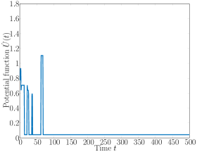
Figure 3: Convergence of the perturbed potential function $\hat{U}(t)$ in (12) for $\delta=0.3065$ to a non-zero value corresponding to a configuration of a Nash equilibrium, that is not a minimizer of the perturbed potential function.

V CONCLUSION

We revisited a distributed learning algorithm for optimal allocation of synchronous and converter-based generators in radial power systems based on log-linear learning with guaranteed probabilistic convergence to Nash equilibrium. Moreover, we investigated its robustness against drops in the line susceptances with respect to a feasible region of power deviations. Future investigations involve the study of general network topology for mixed power generation.

References

- [1] M. Paolone, T. Gaunt, X. Guillaud, M. Liserre, S. Meliopoulos, A. Monti, T. Van Cutsem, V. Vittal, and C. Vournas, “Fundamentals of power systems modelling in the presence of converter-interfaced generation,” Electric Power Systems Research, vol. 189, p. 106811, 2020.
- [2] T. Jouini and Z. Sun, “Performance analysis and optimization of power systems with spatially correlated noise,” IEEE Control Systems Letters, vol. 5, no. 1, pp. 361–366, 2021.
- [3] J. R. Marden and A. Wierman, “Distributed welfare games,” Operations Research, vol. 61, no. 1, pp. 155–168, 2013.
- [4] D. Bauso, Game theory with engineering applications. SIAM, 2016.
- [5] J. Barreiro-Gomez, F. Dörfler, and H. Tembine, “Distributed robust population games with applications to optimal frequency control in power systems,” in 2018 Annual American Control Conference (ACC). IEEE, 2018, pp. 5762–5767.
- [6] P. Chakraborty, E. Baeyens, and P. P. Khargonekar, “Distributed control of flexible demand using proportional allocation mechanism in a smart grid: Game theoretic interaction and price of anarchy,” Sustainable Energy, Grids and Networks, vol. 12, pp. 30–39, 2017.
- [7] W. W. Weaver and P. T. Krein, “Game-theoretic control of small-scale power systems,” IEEE Transactions on Power Delivery, vol. 24, no. 3, pp. 1560–1567, 2009.
- [8] P. Chakraborty, E. Baeyens, K. Poolla, P. P. Khargonekar, and P. Varaiya, “Sharing storage in a smart grid: A coalitional game approach,” IEEE Transactions on Smart Grid, vol. 10, no. 4, pp. 4379–4390, 2018.
- [9] Q. Xu, N. Zhang, C. Kang, Q. Xia, D. He, C. Liu, Y. Huang, L. Cheng, and J. Bai, “A game theoretical pricing mechanism for multi-area spinning reserve trading considering wind power uncertainty,” IEEE Transactions on Power Systems, vol. 31, no. 2, pp. 1084–1095, 2016.
- [10] B. K. Poolla, S. Bolognani, L. Na, and F. Dörfler, “A market mechanism for virtual inertia,” IEEE Transactions on Smart Grid, 2020.
- [11] N. Forouzandehmehr, Z. Han, and R. Zheng, “Stochastic dynamic game between hydropower plant and thermal power plant in smart grid networks,” IEEE Systems Journal, vol. 10, no. 1, pp. 88–96, 2014.
- [12] A. Farraj, E. Hammad, A. A. Daoud, and D. Kundur, “A game-theoretic analysis of cyber switching attacks and mitigation in smart grid systems,” IEEE Transactions on Smart Grid, vol. 7, no. 4, pp. 1846–1855, 2016.
- [13] T. Alpcan and T. Başar, Network security: A decision and game-theoretic approach. Cambridge University Press, 2010.
- [14] D. Fudenberg, F. Drew, D. K. Levine, and D. K. Levine, The theory of learning in games. MIT press, 1998, vol. 2.
- [15] D. Monderer and L. S. Shapley, “Potential games,” Games and economic behavior, vol. 14, no. 1, pp. 124–143, 1996.
- [16] J. R. Marden, G. Arslan, and J. S. Shamma, “Joint strategy fictitious play with inertia for potential games,” IEEE Transactions on Automatic Control, vol. 54, no. 2, pp. 208–220, 2009.
- [17] J. R. Marden and J. S. Shamma, “Revisiting log-linear learning: Asynchrony, completeness and payoff-based implementation,” Games and Economic Behavior, vol. 75, no. 2, pp. 788–808, 2012.
- [18] L. E. Blume et al., “The statistical mechanics of strategic interaction,” Games and economic behavior, vol. 5, no. 3, pp. 387–424, 1993.
- [19] R. Zhang, Y. Du, and L. Yuhong, “New challenges to power system planning and operation of smart grid development in china,” in 2010 International Conference on Power System Technology. IEEE, 2010, pp. 1–8.
- [20] U. Markovic, O. Stanojev, E. Vrettos, P. Aristidou, and G. Hug, “Understanding stability of low-inertia systems,” Feb 2019.
- [21] J. Schiffer, D. Efimov, and R. Ortega, “Almost global synchronization in radial multi-machine power systems,” in Proc. 57th IEEE Conference on Decision and Control (CDC), 2018.
- [22] J. W. Simpson-Porco, F. Dörfler, and F. Bullo, “Synchronization and power sharing for droop-controlled inverters in islanded microgrids,” Automatica, vol. 49, no. 9, pp. 2603–2611, 2013.
- [23] P. Kundur, N. J. Balu, and M. G. Lauby, Power system stability and control. McGraw-hill New York, 1994, vol. 7.
- [24] M. Hasanbeig and L. Pavel, “From game-theoretic multi-agent log linear learning to reinforcement learning,” arXiv preprint arXiv:1802.02277, 2018.
- [25] J. R. Marden, G. Arslan, and J. S. Shamma, “Cooperative control and potential games,” IEEE Transactions on Systems, Man, and Cybernetics, Part B (Cybernetics), vol. 39, no. 6, pp. 1393–1407, 2009.
- [26] T. Ding, R. Bo, Y. Yang, and F. Blaabjerg, “Impact of negative reactance on definiteness of b-matrix and feasibility of dc power flow,” IEEE Transactions on Smart Grid, vol. 10, no. 2, pp. 1725–1734, 2017.
- [27] D. Jones, “Estimation of power system parameters,” IEEE Transactions on Power Systems, vol. 19, no. 4, pp. 1980–1989, 2004.
- [28] S. Guo, S. Norris, and J. Bialek, “Adaptive parameter estimation of power system dynamic model using modal information,” IEEE Transactions on Power Systems, vol. 29, no. 6, pp. 2854–2861, 2014.
- [29] W. Gong, B. Zhang, and C. Li, “Task assignment in mobile crowdsensing: Present and future directions,” IEEE Network, vol. 32, no. 4, pp. 100–107, 2018.
- [30] G. Qu, D. Brown, and N. Li, “Distributed greedy algorithm for multi-agent task assignment problem with submodular utility functions,” Automatica, vol. 105, pp. 206–215, 2019.
- [31] W. Group, “Common format for exchange of solved load flow data,” IEEE Transactions on Power Apparatus and Systems, vol. PAS-92, no. 6, pp. 1916–1925, 1973.