An inverse random source problem for the one-dimensional Helmholtz equation with attenuation

Abstract.

This paper is concerned with an inverse random source problem for the one-dimensional stochastic Helmholtz equation with attenuation. The source is assumed to be a microlocally isotropic Gaussian random field with its covariance operator being a classical pseudo-differential operator. The random sources under consideration are equivalent to the generalized fractional Gaussian random fields which include rough fields and can be even rougher than the white noise, and hence should be interpreted as distributions. The well-posedness of the direct source scattering problem is established in the distribution sense. The micro-correlation strength of the random source, which appears to be the strength in the principal symbol of the covariance operator, is proved to be uniquely determined by the wave field in an open measurement set. Numerical experiments are presented for the white noise model to demonstrate the validity and effectiveness of the proposed method.

1. Introduction

Inverse source problems for wave propagation aim to determine the unknown sources by using supplementary information of the wave field. They arise naturally and have significant applications in diverse fields of science, which include particularly the area of medical and biomedical imaging such as magnetoencephalography [2, 12], optical molecular imaging [3], and fluorescence tomography [10]. Motivated by these applications, inverse source scattering problems have been extensively investigated, and many mathematical and numerical results are available [7, 8, 15, 16].

Recently, to characterize more precisely the uncertainties in unpredictable systems with incomplete knowledge, random sources are taken into consideration in mathematical modeling [4, 5, 11]. As is well known, classical inverse problems are already rather difficult to solve due to the nonlinearity and ill-posedness. Inverse problems with random sources would be more challenging since the ill-posedness is severer compared to their deterministic counterparts: (1) the random source, in some cases, is too rough to exist pointwisely and should be interpreted as distributions instead; (2) the wave field generated by the random source is also a random field. Random fields are determined by their statistics such as the mean and covariance functions. As a result, only statistics of the random source may be reconstructed based on the statistics of the wave field. It is worth pointing out that the statistics of the random source which can be determined and the statistics of the wave field which can be used as proper measurement data depend heavily on the form of the random source, which makes it hard to solve inverse random source problems.

In this paper, we consider the one-dimensional stochastic Helmholtz equation with attenuation

$$u^{\prime\prime}(x)+(k^{2}+{\rm i}k\sigma)u(x)=f(x),\quad x\in\mathbb{R},$$ (1.1)

where $k>0$ is the wave number, the attenuation coefficient $\sigma>0$ describes the electrical conductivity of the medium, $u$ denotes the scattered field, and $f$ represents the electric current density and is assumed to be a random field supported in $D=(0,1)$. In the one-dimensional case, the outgoing radiation condition imposed on $u$ is equivalent to the following boundary conditions:

$$u^{\prime}(0)+{\rm i}\kappa u(0)=0,\quad u^{\prime}(1)+{\rm i}\kappa u(1)=0,$$

which accounts for the left-going wave at $x=0$ and the right-going wave at $x=1$, respectively. Here $\kappa$ satisfies $\kappa^{2}=k^{2}+{\rm i}\sigma k$.

There has been much work on the study of inverse random source problems. When the source takes the form $f=g+h\dot{W}$, where $\dot{W}$ is the spatial white noise, $g$ and $h$ are smooth and compactly supported functions, the random source has independent increments. As a result, the Itô isometry can be used to derive reconstruction formulas which connect the statistics of the random source to those of the wave field, and the functions $g$ and $h$ can be determined based on the measurement data at multiple frequencies. We refer to [4, 6, 21] for the study on the stochastic Helmholtz equation without attenuation and to [5] for the study on the stochastic elastic wave equation.

More generally, another important class of random sources, known as the microlocally isotropic Gaussian random fields, is considered in [17, 18, 19, 20, 22, 23]. The covariance operators of the random fields are assumed to be pseudo-differential operators with principal symbol $\mu(x)|\xi|^{-m}$, where the nonnegative function $\mu\in C_{0}^{\infty}(D)$ is called the micro-correlation strength of the random source and is the statistics to be determined. It is shown in [22] that the microlocally isotropic Gaussian random field is equivalent to the generalized fractional Gaussian random field in the form

$$f=\sqrt{\mu}(-\Delta)^{-\frac{m}{4}}\dot{W},$$

which is a distribution in $W^{\frac{m-d}{2}-\epsilon,p}(\mathbb{R}^{d})$ for $m\in(-\infty,d]$ (cf. Lemma 2.1) and apparently degenerates to the white noise if $m=0$. In this case, the increments of the random source are not independent if $m\neq 0$, and thus the Itô isometry is not applicable any more. Instead, the microlocal analysis for large frequencies is applied to reconstruct the micro-correlation strength $\mu$ involved in the principal symbol of the covariance operator of $f$. In [22], the $d$-dimensional Helmholtz equation with attenuation is studied with $d=2,3$, $p\in(\frac{d}{2},2]$ and $m\in(d(\frac{2}{p}+1)-2,d]$. We refer to [18, 19] for the study on the Helmholtz equation without attenuation and the elastic wave equation, to [20] for the study on the Schrödinger equation, and to [23] for the study on Maxwell’s equations. In all of the existing results, the random source under consideration is smoother than the white noise, i.e., $m>0$, due to the singularity of Green’s functions of the considered models.

In this work, we consider the one-dimensional stochastic Helmholtz equation (1.1) with attenuation, where $f$ is assumed to be a microlocally isotropic Gaussian random field with $m\in(-\frac{2}{q},1]$ and $q\in(1,\infty)$. We point out that such a random source model includes the white noise case with $m=0$ and is even allowed to be rougher than the white noise for $m\in(-\frac{2}{q},0)$. The direct scattering problem is shown to be well-posed in the distribution sense and has a unique solution $u\in W^{\gamma,q}_{loc}(\mathbb{R})$ with $\gamma\in(\frac{1-m}{2},\frac{1}{2}+\frac{1}{q})$. For the inverse scattering problem, we prove that the strength $\mu$ of the random source is uniquely determined by the high frequency limit of the energy of the wave field $u$ on an bounded measurement interval $U\subset\mathbb{R}\backslash\overline{D}$. In particular, for the white noise case, the measurement data at a single frequency is enough to uniquely determine the strength $\mu$ by utilizing the Itô isometry. Numerical experiments are presented for the white noise model to demonstrate the validity and effectiveness of the proposed method.

The paper is organized as follows. In Section 2, the microlocally isotropic random source is introduced. The well-posedness of the direct scattering problem in the distribution sense is given based on the regularity of the fundamental solution. Section 3 concerns the inverse scattering problem. The uniqueness is addressed for the reconstruction of the strength of the random source. As a special case of the microlocally isotropic random source, the white noise model is studied in Section 4. Numerical experiments are presented in Section 5 to demonstrate the effectiveness of the proposed method. The paper is concluded with some general remarks in Section 6.

2. Direct scattering problem

In this section, we introduce the model of the random source and present the well-posedness and stability of the solution for the direct scattering problem.

2.1. Random sources

The source $f$ is assumed to be a microlocally isotropic Gaussian random field which satisfies the following conditions with dimension $d=1$.

Assumption 1.

Let $f$ be a real-valued centered microlocally isotropic Gaussian random field of order $-m$ compactly supported in $D\subset\mathbb{R}^{d}$, i.e., the covariance operator of $f$ is a pseudo-differential operator whose principal symbol has the form $\mu(x)|\xi|^{-m}$ with the micro-correlation strength $\mu\in C_{0}^{\infty}(D)$ and $\mu\geq 0$.

It is shown in [22, Proposition 2.5] that the generalized Gaussian random field

$$f(x)=\sqrt{\mu(x)}(-\Delta)^{-\frac{m}{4}}\dot{W}$$

satisfies Assumption 1 with order $-m$, where $\dot{W}$ is the white noise and $(-\Delta)^{-\frac{m}{4}}$ is a fractional Laplacian. Consequently, the regularity of random fields satisfying Assumption 1 can be obtained by investigating the regularity of the generalized Gaussian random fields, which is stated in the following lemma (cf. [22]).

Lemma 2.1.

Let $f$ be a microlocally isotropic Gaussian random field of order $-m$ compactly supported in $D\subset\mathbb{R}^{d}$.

• If $m\in(d,d+2)$, then $f\in C^{\alpha}(D)$ almost surely for all $\alpha\in(0,\frac{m-d}{2})$.

• If $m\in(-\infty,d]$, then $f\in W^{\frac{m-d}{2}-\epsilon,p}(D)$ almost surely for all $\epsilon>0$ and $p\in(1,\infty)$.

Let $\mathcal{D}$ be the space $C_{0}^{\infty}(\mathbb{R}^{d})$ equipped with a locally convex topology, and $\mathcal{D}^{\prime}$ be its dual space. Based on Lemma 2.1, if $m\leq d$, the random source $f$ should be interpreted as a distribution in $\mathcal{D}^{\prime}$. Its mean value function, denoted by $E_{f}$, and covariance operator, denoted by $Q_{f}$, are defined as follows:

$$\langle E_{f},\varphi\rangle: = \mathbb{E}\langle f,\varphi\rangle\quad\forall~{}\varphi\in\mathcal{D},$$

$$\langle\varphi,Q_{f}\psi\rangle: = \mathbb{E}[\langle f,\varphi\rangle\langle f,\psi\rangle]\quad\forall~{}\varphi,\psi\in\mathcal{D},$$

where $\langle\cdot,\cdot\rangle$ denotes the dual product. According to the Schwartz kernel theorem (cf. [13, Theorem 5.2.1]), there exists a unique kernel $K_{f}$ for $Q_{f}$ such that

$$\langle\varphi,Q_{f}\psi\rangle=\int_{\mathbb{R}^{d}}\int_{\mathbb{R}^{d}}K_{f}(x,y)\varphi(x)\psi(y)dxdy.$$ (2.1)

If $f$ satisfies Assumption 1, then its covariance operator $Q_{f}$ is a pseudo-differential operator with the principal symbol given by $\mu(x)|\xi|^{-m}$, and hence (cf. [14])

$$(Q_{f}\psi)(x)=\frac{1}{(2\pi)^{d}}\int_{\mathbb{R}^{d}}e^{{\rm i}x\cdot\xi}c(x,\xi)\hat{\psi}(\xi)d\xi,$$

where $c(x,\xi)$ is the symbol of $Q_{f}$ with the leading term $\mu(x)|\xi|^{-m}$ and

$$\hat{\psi}(\xi)=\mathcal{F}[\psi](\xi)=\int_{\mathbb{R}^{d}}e^{-{\rm i}x\cdot\xi}\psi(x)dx$$

is the Fourier transform of $\psi$. It then holds

$$\langle\varphi,Q_{f}\psi\rangle = \int_{{\mathbb{R}}^{d}}\varphi(x)\left[\frac{1}{(2\pi)^{d}}\int_{{\mathbb{R}}^{d}}e^{{\rm i}x\cdot\xi}c(x,\xi)\hat{\psi}(\xi)d\xi\right]dx$$

$$= \frac{1}{(2\pi)^{d}}\int_{{\mathbb{R}}^{d}}\varphi(x)\int_{{\mathbb{R}}^{d}}e^{{\mathbf{i}}x\cdot\xi}c(x,\xi)\left[\int_{{\mathbb{R}}^{d}}e^{-{\rm i}y\cdot\xi}\psi(y)dy\right]d\xi dx$$

$$= \int_{{\mathbb{R}}^{d}}\int_{{\mathbb{R}}^{d}}\left[\frac{1}{(2\pi)^{d}}\int_{{\mathbb{R}}^{d}}e^{{\rm i}(x-y)\cdot\xi}c(x,\xi)d\xi\right]\varphi(x)\psi(y)dxdy.$$

Comparing the above equation with (2.1), we get that the kernel $K_{f}$ is an oscillatory integral of the form

$$K_{f}(x,y)=\frac{1}{(2\pi)^{d}}\int_{{\mathbb{R}}^{d}}e^{{\rm i}(x-y)\cdot\xi}c(x,\xi)d\xi,$$ (2.2)

which is determined by the symbol $c(x,\xi)$.

2.2. The fundamental solution

Define the complex wave number $\kappa$ such that $\kappa^{2}=k^{2}+{\rm i}k\sigma$, whose real and imaginary parts $\kappa_{\rm r}$ and $\kappa_{\rm i}$ satisfy

$$\kappa_{\rm r}=\left(\frac{\sqrt{k^{4}+k^{2}\sigma^{2}}+k^{2}}{2}\right)^{\frac{1}{2}},\quad\kappa_{\rm i}=\left(\frac{\sqrt{k^{4}+k^{2}\sigma^{2}}-k^{2}}{2}\right)^{\frac{1}{2}}.$$

It is easy to verify that

$$\lim_{k\to\infty}\frac{\kappa_{\rm r}}{k}=1,\quad\lim_{k\to\infty}\kappa_{\rm i}=\frac{\sigma}{2}.$$ (2.3)

Before showing the well-posedness of the solution for the random equation (1.1), we recall that the equation

$$(\partial_{xx}+\kappa^{2})\Phi_{\kappa}(x,y)=-\delta(x-y),\quad x,y\in\mathbb{R}$$

admits a unique solution

$$\Phi_{\kappa}(x,y)=\frac{{\rm i}}{2\kappa}e^{{\rm i}\kappa|x-y|},$$

which is the fundamental solution for the one-dimensional Helmholtz equation.

For any $n\in\mathbb{N}$, denote by $W^{n,p}(\mathcal{O})$ the Sobolev space equipped with the norm

$$\|v\|_{W^{n,p}(\mathcal{O})}:=\left(\sum_{0\leq\alpha\leq n}\|\partial^{\alpha}v\|_{L^{p}(\mathcal{O})}^{p}\right)^{\frac{1}{p}}.$$

Let $W^{n,p}_{0}(\mathcal{O})$ be the closure of $C_{0}^{\infty}(\mathcal{O})$ in $W^{n,p}(\mathcal{O})$ and $W^{-n,q}(\mathcal{O})=(W^{n,p}_{0}(\mathcal{O}))^{\prime}$ be the dual space of $W^{n,p}_{0}(\mathcal{O})$ with $\frac{1}{p}+\frac{1}{q}=1$. We refer to [1] for more details on these Sobolev spaces.

The fundamental solution $\Phi_{\kappa}$ has the following regularity property.

Lemma 2.2.

For any given $x\in\mathbb{R}$ and $p\in(1,\infty)$, it holds $\Phi_{\kappa}(x,\cdot)\in W_{loc}^{1,p}(\mathbb{R}).$

Proof.

Let $\mathcal{O}\subset\mathbb{R}$ be any bounded interval with a finite Lebesgue measure which is denoted by $C_{\mathcal{O}}$. It suffices to show that $\Phi_{\kappa}(x,\cdot),\partial\Phi_{\kappa}(x,\cdot)\in L^{p}(\mathcal{O})$. A simple calculation gives

$$\|\Phi_{\kappa}(x,\cdot)\|_{L^{p}(\mathcal{O})}^{p} = \int_{\mathcal{O}}\left|\frac{{\rm i}}{2\kappa}e^{{\rm i}\kappa|x-y|}\right|^{p}dy=\int_{\mathcal{O}}\left(\frac{1}{2|\kappa|}\right)^{p}e^{-p\kappa_{\rm i}|x-y|}dy$$

$$\leq (2|\kappa|)^{-p}C_{\mathcal{O}}.$$

Since the classical partial derivative of $\Phi_{\kappa}(x,y)$ with respect to $y$ exists, we have

$$\partial_{y}\Phi_{\kappa}(x,y)=\frac{x-y}{2|x-y|}e^{{\rm i}\kappa|x-y|},\quad y\neq x.$$

It is clear to note

$$\|\partial\Phi_{\kappa}(x,\cdot)\|_{L^{p}(\mathcal{O})}^{p}=\frac{1}{2^{p}}\int_{\mathcal{O}}e^{-p\kappa_{\rm i}|x-y|}dy\leq 2^{-p}C_{\mathcal{O}},$$

which completes the proof. ∎

2.3. Well-posedness and regularity

Based on the fundamental solution $\Phi_{\kappa}$, the volume potential

$$(H_{\kappa}v)(x):=-\int_{\mathbb{R}}\Phi_{\kappa}(x,y)v(y)dy$$ (2.4)

defines a mollifier $H_{\kappa}$.

Lemma 2.3.

Let $\mathcal{O},\mathcal{V}\subset\mathbb{R}$ be any two bounded intervals. The operator $H_{\kappa}:H^{-\beta}(\mathcal{O})\to H^{\beta}(\mathcal{V})$ is bounded for $\beta\in(0,1]$.

Proof.

It follows from [9, Theorem 8.1] that $H_{\kappa}$ is bounded from $C(\mathcal{O})$ to $C^{2}(\mathcal{V})$ with respect to the norms

$$\|v\|_{C(\mathcal{O})}:=\sup_{x\in\mathbb{R}}|v(x)|\quad\forall~{}v\in C(\mathcal{O})$$

and

$$\|v\|_{C^{2}(\mathcal{V})}:=\sum_{m=0}^{2}\sup_{x\in\mathbb{R}}|v^{(m)}(x)|\quad\forall~{}v\in C^{2}(\mathcal{V}).$$

Define spaces $X:=C(\mathcal{O})$ and $Y:=C^{2}(\mathcal{V})$ with the scalar products given by

$$(g_{1},g_{2})_{X}:=(\tilde{g}_{1},\tilde{g}_{2})_{H^{\beta-2}(\mathbb{R})}\quad\forall\,g_{1},g_{2}\in X$$

and

$$(h_{1},h_{2})_{Y}:=(\tilde{h}_{1},\tilde{h}_{2})_{H^{\beta}(\mathbb{R})}\quad\forall\,h_{1},h_{2}\in Y,$$

respectively, where $\tilde{g}_{i}$ and $\tilde{h}_{i}$ are the zero extensions of $g_{i}$ and $h_{i}$ in $\mathbb{R}\setminus\overline{\mathcal{O}}$ and $\mathbb{R}\setminus\overline{\mathcal{V}}$, respectively. It is easy to verify that the products defined above satisfy

$$(g_{1},g_{2})_{X} = (J^{\beta-2}\tilde{g}_{1},J^{\beta-2}\tilde{g}_{2})_{L^{2}(\mathbb{R})}=\int_{\mathbb{R}}(1+\xi^{2})^{\beta-2}\hat{\tilde{g}}_{1}(\xi)\overline{\hat{\tilde{g}}_{2}(\xi)}d\xi$$

$$\lesssim \|\tilde{g}_{1}\|_{L^{2}(\mathbb{R})}\|\tilde{g}_{2}\|_{L^{2}(\mathbb{R})}\lesssim\|g_{1}\|_{C(\mathcal{O})}\|g_{2}\|_{C(\mathcal{O})}$$

and

$$(h_{1},h_{2})_{Y} = (J^{\beta}\tilde{h}_{1},J^{\beta}\tilde{h}_{2})_{L^{2}(\mathbb{R})}=\int_{\mathbb{R}}(1+\xi^{2})^{\beta}\hat{\tilde{h}}_{1}(\xi)\overline{\hat{\tilde{h}}_{2}(\xi)}d\xi$$

$$\lesssim \|\tilde{h}_{1}\|_{H^{\beta}(\mathbb{R})}\|\tilde{h}_{2}\|_{H^{\beta}(\mathbb{R})}\lesssim\|h_{1}\|_{C^{2}(\mathcal{V})}\|h_{2}\|_{C^{2}(\mathcal{V})}.$$

We claim that there exists a bounded operator $V:Y\to X$ defined by

$$V:=(I-\partial_{xx})\overline{H_{\kappa}}(I-\partial_{xx}),$$

where

$$(\overline{H_{\kappa}}v)(x):=-\int_{\mathbb{R}}\overline{\Phi_{\kappa}(x,y)}v(y)dy$$

and $\overline{H_{\kappa}}v=\overline{H_{\kappa}v}$ for any real valued function $v$, such that

$$(H_{\kappa}g,h)_{Y}=(g,Vh)_{X}\quad\forall\,g\in X,h\in Y.$$

In fact, for any $h\in Y$,

$$\|Vh\|_{C(\mathcal{O})} = \|(I-\partial_{xx})\overline{H_{\kappa}}(I-\partial_{xx})h\|_{C(\mathcal{O})}\lesssim\|H_{\kappa}(I-\partial_{xx})h\|_{C^{2}(\mathcal{O})}$$

$$\lesssim \|(I-\partial_{xx})h\|_{C(\mathcal{V})}\lesssim\|h\|_{C^{2}(\mathcal{V})}.$$

Furthermore,

$$(H_{\kappa}g,h)_{Y} = (J^{\beta}H_{\kappa}\tilde{g},J^{\beta}\tilde{h})_{L^{2}(\mathbb{R})}=(H_{\kappa}\tilde{g},J^{2\beta}\tilde{h})_{L^{2}(\mathbb{R})}$$

$$= (\widehat{H_{\kappa}\tilde{g}},\widehat{J^{\beta}\tilde{h}})_{L^{2}(\mathbb{R})}=\int_{\mathbb{R}}\hat{\Phi}_{\kappa}(\xi)\hat{\tilde{g}}(\xi)(1+\xi^{2})^{\beta}\overline{\hat{\tilde{h}}(\xi)}d\xi$$

$$= \int_{\mathbb{R}}\hat{\tilde{g}}(\xi)(1+\xi^{2})^{\beta-2}\overline{\left[(1+\xi^{2})\overline{\hat{\Phi}_{\kappa}(\xi)}(1+\xi^{2})\hat{\tilde{h}}(\xi)\right]}d\xi$$

$$= \int_{\mathbb{R}}\hat{\tilde{g}}(\xi)(1+\xi^{2})^{\beta-2}\overline{\widehat{V\tilde{h}}(\xi)}d\xi=(J^{\beta-2}\tilde{g},J^{\beta-2}V\tilde{h})_{L^{2}(\mathbb{R})}$$

$$= (g,Vh)_{X},$$

where $\hat{\Phi}_{\kappa}$ is the Fourier transform of $\Phi_{\kappa}(x,y)$ with respect to $x-y$ and satisfies $-\xi^{2}\hat{\Phi}_{\kappa}(\xi)+\kappa^{2}\hat{\Phi}_{\kappa}(\xi)=-1$. The claim is proved.

It follows from the claim and [9, Theorem 3.5] that $H_{\kappa}:X\to Y$ is bounded with respect to the norms induced by the scalar products on $X$ and $Y$. More precisely, we have

$$\|H_{\kappa}g\|_{Y}=\|H_{\kappa}g\|_{H^{\beta}(\mathcal{V})}\lesssim\|g\|_{X}=\|g\|_{H^{\beta-2}(\mathcal{O})}\leq\|g\|_{H^{-\beta}(\mathcal{O})}$$ (2.5)

for any $g\in X$ and $\beta\leq 1$. It then suffices to show that (2.5) also holds for any $g\in H^{-\beta}(\mathcal{O})$. Noting that the subspace $C_{0}^{\infty}(\mathcal{O})\subset X$ is dense in $L^{2}(\mathcal{O})$ (cf. [1, Section 2.30]) and $H^{-1}(\mathcal{O})=\overline{L^{2}(\mathcal{O})}^{\|\cdot\|_{H^{-1}(\mathcal{O})}}$ (cf. [1, Section 3.13]), we get that (2.5) holds for any $g\in H^{-1}(\mathcal{O})$, and hence for any $g\in H^{-\beta}(\mathcal{O})$ since $H^{-\beta}(\mathcal{O})\subset H^{-1}(\mathcal{O})$. ∎

Now we are able to show the well-posedness of (1.1) in the distribution sense.

Theorem 2.4.

Let $q\in(1,\infty)$ and Assumption 1 hold with $m\in(-\frac{2}{q},1]$. The scattering problem (1.1) has a unique solution

$$u(x)=-\int_{D}\Phi_{\kappa}(x,y)f(y)dy$$

in the distribution sense, and $u\in W^{\gamma,q}_{loc}(\mathbb{R})$ almost surely with $\gamma\in(\frac{1-m}{2},\frac{1}{2}+\frac{1}{q})$.

Proof.

We first show that the volume potential

$$u(x)=-\int_{D}\Phi_{\kappa}(x,y)f(y)dy=(H_{\kappa}f)(x)$$

is well-defined in $W^{\gamma,q}_{loc}(\mathbb{R})$, i.e., $u\in W^{\gamma,q}(K)$ for any compact subset $K\subset\mathbb{R}$. It follows from the Kondrachov embedding theorem that the following embeddings

$$W^{-\gamma,p}(D)\hookrightarrow H^{-\beta}(D),\quad H^{\beta}(K)\hookrightarrow W^{\gamma,q}(K)$$

with $\beta=1$ and $\frac{1}{p}+\frac{1}{q}=1$ are compact. Hence, $H_{\kappa}:W^{-\gamma,p}(D)\to W^{\gamma,q}(K)$ is bounded based on Lemma 2.3. By Lemma 2.1, it is clear to note that $f\in W^{\frac{m-1}{2}-\epsilon,p}(D)\subset W^{-\gamma,p}(D)$. As a result, $u=H_{\kappa}f\in W^{\gamma,q}(K)$.

Next, we prove that $u=H_{\kappa}f$ is a solution to (1.1) in the distribution sense. For any test function $v\in W^{\gamma,q}(\mathbb{R})$, it holds

$$\langle u^{\prime\prime}+\kappa^{2}u,v\rangle=-\langle u^{\prime},v^{\prime}\rangle+\kappa^{2}\langle u,v\rangle$$

$$= \int_{\mathbb{R}}\partial_{x}\Big{[}\int_{D}\Phi_{\kappa}(x,y)f(y)dy\Big{]}v^{\prime}(x)dx-\kappa^{2}\int_{\mathbb{R}}\Big{[}\int_{D}\Phi_{\kappa}(x,y)f(y)dy\Big{]}v(x)dx$$

$$= -\int_{D}\int_{\mathbb{R}}\partial_{xx}\Phi_{\kappa}(x,y)v(x)f(y)dxdy-\kappa^{2}\int_{\mathbb{R}}\Big{[}\int_{D}\Phi_{\kappa}(x,y)f(y)dy\Big{]}v(x)dx$$

$$= \int_{D}\int_{\mathbb{R}}\left(\kappa^{2}\Phi_{\kappa}(x,y)+\delta(x-y)\right)v(x)f(y)dxdy$$

$$-\kappa^{2}\int_{\mathbb{R}}\Big{[}\int_{D}\Phi_{\kappa}(x,y)f(y)dy\Big{]}v(x)dx$$

$$= \langle f,v\rangle.$$

The uniqueness of the solution of (1.1) can be proved by showing that (1.1) has only the zero solution if $f\equiv 0$. Let $u^{0}$ be any solution of (1.1) with $f\equiv 0$ in the distribution sense. Then $u^{0}$ satisfies

$$(u^{0})^{\prime\prime}+\kappa^{2}u^{0}=0$$

in the distribution sense. Denote $B_{r}=(-r,r)$. It is shown in Lemma 2.2 that $\Phi_{\kappa}(x,\cdot)\in W^{1,p^{\prime}}(B_{r})\hookrightarrow W^{\gamma,q}(B_{r})$ for some $p^{\prime}>1$ satisfying $\frac{1}{p^{\prime}}-(1-\gamma)<\frac{1}{q}$. It then indicates that $1_{B_{r}}\Phi_{\kappa}(x,\cdot)\in W^{\gamma,q}(\mathbb{R})$, where $1_{B_{r}}$ denotes the characteristic function. Hence, we get

$$\int_{\mathbb{R}}\Phi_{\kappa}(x,z)\left[(u^{0})^{\prime\prime}(z)+\kappa^{2}u^{0}(z)\right]dz=0.$$ (2.6)

Define the operator $T$ by

$$(T\psi)(x):=\int_{B_{r}}\Phi_{\kappa}(x,z)[\psi^{\prime\prime}(z)+\kappa^{2}\psi(z)]dz\quad\forall\,\psi\in\mathcal{D}.$$

Following the similar arguments as those in the proof of [18, Lemma 4.3] and using the integration by parts, we obtain

$$(T\psi)(x)=-\psi(x)+\left[\Phi_{\kappa}(x,z)\psi^{\prime}(z)-\partial_{z}\Phi_{\kappa}(x,z)\psi(z)\right]\big{|}_{z=-r}^{r}.$$

Then (2.6) leads to

$$-u^{0}(x)+\lim_{r\to\infty}\left[\Phi_{\kappa}(x,z)(u^{0})^{\prime}(z)-\partial_{z}\Phi_{\kappa}(x,z)u^{0}(z)\right]\big{|}_{z=-r}^{r}=0.$$

Applying the radiation condition, we get $u^{0}\equiv 0$, which completes the proof. ∎

3. Inverse scattering problem

By Theorem 2.4, the solution of (1.1) has the form

$$u(x)=\frac{1}{2{\rm i}\kappa}\int_{D}e^{{\rm i}\kappa|x-y|}f(y)dy.$$ (3.1)

We show that the micro-correlation strength $\mu$ is uniquely determined by the variance of the solution $u$.

Theorem 3.1.

Let $f$ be a random source satisfying Assumption 1 and $U\subset\mathbb{R}\setminus\overline{D}$ be a bounded open interval. Then for any$x\in U$,

$$\lim_{k\to\infty}4k^{m+2}{\mathbb{E}}|u(x)|^{2}=\int_{D}e^{-\sigma|x-y|}\mu(y)dy=:T(x).$$

Proof.

Since $U$ and $D$ are disjoint, we first consider the case $x>y$ for any $x\in U$ and $y\in D$. Using (3.1) and the fact that $f$ is compactly supported in $D$, we have for any $x\in U$ that

$${\mathbb{E}}|u(x)|^{2} = \frac{1}{4|\kappa|^{2}}\int_{D}\int_{D}e^{{\rm i}\kappa|x-y|-{\rm i}\bar{\kappa}|x-z|}{\mathbb{E}}[f(y)f(z)]dydz$$

$$= \frac{1}{4|\kappa|^{2}}\int_{D}\int_{D}e^{{\rm i}\kappa(x-y)-{\rm i}\bar{\kappa}(x-z)}K_{f}(y,z)\theta(x)dydz$$

$$= \frac{1}{4|\kappa|^{2}}\int_{\mathbb{R}}\int_{\mathbb{R}}e^{\kappa_{\rm i}(y+z-2x)-{\rm i}\kappa_{\rm r}(y-z)}C_{1}(y,z,x)dydz,$$

where $\theta\in C_{0}^{\infty}(\mathbb{R})$ such that $\theta|_{U}\equiv 1$ and supp$(\theta)\subset{\mathbb{R}}\backslash\overline{D}$,

$$C_{1}(y,z,x):=K_{f}(y,z)\theta(x)=\frac{1}{2\pi}\int_{{\mathbb{R}}}e^{{\rm i}(y-z)\xi}c_{1}(y,x,\xi)d\xi.$$

Here $c_{1}(y,x,\xi):=c(y,\xi)\theta(x)$ and $c(y,\xi)$ is the symbol of the covariance operator of $f$. Then according to Assumption 1, the principal symbol of $c_{1}$ has the form

$$c_{1}^{p}(y,x,\xi)=\mu(y)\theta(x)|\xi|^{-m}.$$

First we define an invertible transformation $\tau:{\mathbb{R}}^{3}\to{\mathbb{R}}^{3}$ by $\tau(y,z,x)=(g,h,x)$, where

$$g=y-z,\quad h=y+z.$$

It follows from a straightforward calculation that

$${\mathbb{E}}|u(x)|^{2}=\frac{1}{4|\kappa|^{2}}\int_{\mathbb{R}}\int_{\mathbb{R}}e^{\kappa_{\rm i}h-2\kappa_{\rm i}x-{\rm i}\kappa_{\rm r}g}C_{2}(g,h,x)dgdh,$$

where

$$C_{2}(g,h,x) = C_{1}(\tau^{-1}(g,h,x))|\det\left((\tau^{-1})^{\prime}(g,h,x)\right)|$$

$$= \frac{1}{2}C_{1}\left(\frac{g+h}{2},\frac{h-g}{2},x\right)$$

$$= \frac{1}{4\pi}\int_{\mathbb{R}}e^{{\rm i}g\xi}c_{1}\Big{(}\frac{g+h}{2},x,\xi\Big{)}d\xi$$

$$= \frac{1}{4\pi}\int_{\mathbb{R}}e^{{\rm i}g\xi}c_{2}\Big{(}h,x,\xi\Big{)}d\xi.$$

Here in the last step, we have used the following asymptotic expansion of symbols (cf. [14, Lemma 18.2.1]):

$$c_{2}(h,x,\xi) = e^{-{\rm i}\left\langle D_{g},D_{\xi}\right\rangle}c_{1}\Big{(}\frac{g+h}{2},x,\xi\Big{)}\Big{|}_{g=0}$$

$$= \sum_{j=0}^{\infty}\frac{\langle-{\rm i}D_{g},D_{\xi}\rangle^{j}}{j!}c_{1}\Big{(}\frac{g+h}{2},x,\xi\Big{)}\Big{|}_{g=0}.$$

Therefore, the principal symbol of $c_{2}$ has the form

$$c_{2}^{p}(h,x,\xi)=c_{1}^{p}\Big{(}\frac{g+h}{2},x,\xi\Big{)}\Big{|}_{g=0}=\mu\Big{(}\frac{h}{2}\Big{)}|\xi|^{-m}\theta(x),$$

and the residual $r_{2}=c_{2}-c_{2}^{p}\in S^{-m-1}$.

Combining the above equations leads to

$${\mathbb{E}}|u(x)|^{2} = \frac{1}{4|\kappa|^{2}}\int_{\mathbb{R}}\int_{\mathbb{R}}e^{\kappa_{\rm i}h-2\kappa_{\rm i}x-{\rm i}\kappa_{\rm r}g}C_{2}(g,h,x)dgdh$$

$$= \frac{1}{4|\kappa|^{2}}\int_{\mathbb{R}}\int_{\mathbb{R}}e^{\kappa_{\rm i}h-2\kappa_{\rm i}x-{\rm i}\kappa_{\rm r}g}\left[\frac{1}{4\pi}\int_{\mathbb{R}}e^{{\rm i}g\xi}c_{2}\Big{(}h,x,\xi\Big{)}d\xi\right]dgdh$$

$$= \frac{1}{8|\kappa|^{2}}\int_{\mathbb{R}}\int_{\mathbb{R}}e^{\kappa_{\rm i}h-2\kappa_{\rm i}x}\left[\frac{1}{2\pi}\int_{\mathbb{R}}e^{{\rm i}g(\xi-\kappa_{\rm r})}dg\right]c_{2}(h,x,\xi)d\xi dh$$

$$= \frac{1}{8|\kappa|^{2}}\int_{\mathbb{R}}e^{\kappa_{\rm i}h-2\kappa_{\rm i}x}c_{2}(h,x,\kappa_{\rm r})dh$$

$$= \frac{1}{8|\kappa|^{2}}\int_{\mathbb{R}}e^{\kappa_{\rm i}h-2\kappa_{\rm i}x}\bigg{[}\mu\Big{(}\frac{h}{2}\Big{)}\kappa_{\rm r}^{-m}\theta(x)+r_{2}(h,x,\kappa_{\rm r})\bigg{]}dh$$

$$= \frac{\theta(x)}{4|\kappa|^{2}\kappa_{\rm r}^{m}}\int_{\mathbb{R}}e^{2\kappa_{\rm i}(\zeta-x)}\mu(\zeta)d\zeta+O(\kappa_{\rm r}^{-m-1}|\kappa|^{-2}).$$

Finally, for any $x\in U$, we have from (2.3) that

$$\lim_{k\to\infty}4k^{m+2}{\mathbb{E}}|u(x)|^{2}=\lim_{k\to\infty}\left(\frac{k^{m+2}}{|\kappa|^{2}\kappa_{\rm r}^{m}}\right)\int_{D}e^{2\kappa_{\rm i}(\zeta-x)}\mu(\zeta)d\zeta=T(x).$$

On the other hand, if $x<y$ for any $x\in U$ and $y\in D$, we may repeat the same procedure as above and show that

$$\lim_{k\to\infty}4k^{m+2}{\mathbb{E}}|u(x)|^{2}=\lim_{k\to\infty}\left(\frac{k^{m+2}}{|\kappa|^{2}\kappa_{\rm r}^{m}}\right)\int_{D}e^{2\kappa_{\rm i}(x-\zeta)}\mu(\zeta)d\zeta=T(x),$$

which completes the proof. ∎

Now we are in the position to show that the strength $\mu$ of the covariance operator the random source is uniquely determined by the integral given in Theorem 3.1.

Theorem 3.2.

Let $\sigma>0$. The strength $\mu$ is uniquely determined by

$$T(x)=\int_{D}e^{-\sigma|x-y|}\mu(y)dy,\quad x\in U,$$

where $U\subset\mathbb{R}\backslash\overline{D}$ is a bounded interval containing points from both sides of the interval $D$.

Proof.

Let $g(x):=e^{-\sigma|x|}$. Then

$$T(x)=(g*\mu)(x),\quad x\in U,$$ (3.2)

and $T=g*\mu$ is a real analytic function. Hence, the value of $T$ can be obtained everywhere according to the analytic continuation. Taking the Fourier transform of (3.2) yields

$$\mathcal{F}[\mu](\xi)=\frac{\mathcal{F}[T](\xi)}{\mathcal{F}[g](\xi)}=\frac{\sigma^{2}+\xi^{2}}{2\sigma}\mathcal{F}[T](\xi),$$

which implies that $\mu$ can be uniquely determined by $T$. ∎

4. White noise

In this section, we study the inverse random source problem where the source is driven by a white noise. Specifically, we consider a centered random source given in the form

$$f=\sqrt{\mu}\dot{W},$$

where $\dot{W}$ is the real-valued spatial white noise. The diffusion function $\sqrt{\mu}$ is assumed to be a smooth function compactly supported in the interval $D:=(0,1)$. By Lemma 2.1, it holds $f\in W^{-\frac{1}{2}-\epsilon,p}(D)$ for any $\epsilon>0$ and $p\in(1,\infty)$, which has the same regularity as the microlocally isotropic Gaussian random field with $m=0$. Moreover, the covariance operator $Q_{f}$ of $f$ satisfies

$$\langle\varphi,Q_{f}\psi\rangle = \mathbb{E}[\langle\sqrt{\mu}\dot{W},\varphi\rangle\langle\sqrt{\mu}\dot{W},\psi\rangle]$$

$$= \int_{0}^{1}\mu(y)\varphi(y)\psi(y)dy,$$

which implies that

$$K_{f}(x,y)=\mu(y)\delta(x-y)=\frac{1}{2\pi}\int_{\mathbb{R}}e^{{\rm i}(x-y)\xi}\mu(x)d\xi$$

and hence the symbol of $Q_{f}$ is $c(x,\xi)=\mu(x)$ according to (2.2). As a result, $f=\sqrt{\mu}\dot{W}$ satisfies Assumption 1 with $m=0$.

In this case, the solution $u$ of (1.1) is expressed by

$$u(x)=(H_{\kappa}f)(x)=\frac{1}{2{\rm i}\kappa}\int_{0}^{1}e^{{\rm i}\kappa|x-y|}\sqrt{\mu(y)}dW(y).$$ (4.1)

By Itô’s formula, we get

$$\mathbb{E}|u(x)|^{2}=\frac{1}{4|\kappa|^{2}}\int_{0}^{1}e^{-2\kappa_{\rm i}|x-y|}\mu(y)dy,$$

which implies the uniqueness of determining the strength $\mu$ by following the same procedure as that in the proof of Theorem 3.2.

Corollary 4.1.

Let $D:=(0,1)$. If the random source $f$ has the form $f=\sqrt{\mu}\dot{W}$ with strength $\mu\in C_{0}^{\infty}(D)$ and $\mu\geq 0$, then the strength $\mu$ can be uniquely determined by the following data at any fixed wave number $k$:

$$4|\kappa|^{2}\mathbb{E}|u(x)|^{2}=\int_{0}^{1}e^{-2\kappa_{\rm i}|x-y|}\mu(y)dy,\quad x\in U,$$ (4.2)

where $U\subset\mathbb{R}\backslash\overline{D}$ is a bounded interval containing points from both sides of the interval $D$.

5. Numerical experiments

In this section, we present the algorithmic implementation for the direct and inverse scattering problems where the source is driven by the white noise, and show some numerical examples to demonstrate the validity and effectiveness of the proposed method.

5.1. The scattering data

The measurement interval is chosen as $U=[-1.2,-0.2]\cup[1.2,2.2]$ which satisfies $U\subset\mathbb{R}\backslash\overline{D}$ with $D=(0,1)$. The scattering data $u(x)$ for all $x\in U$ is obtained by using the integral equation (4.1). Numerically, we generate the synthetic data at discrete points $\{x_{m}\}_{m=0}^{M+1}\subset U$ defined by

$$x_{0}=-1.2,\quad x_{\frac{M}{2}+2}=1.2,\quad x_{m+1}=x_{m}+\Delta x$$

for $m=0,\cdots,\frac{M}{2},\frac{M}{2}+2,\cdots,M$ with $M=200$ and $\Delta x=2/M$, and approximate $u(x_{m})$ by

$$u(x_{m})\approx\frac{1}{2{\rm i}\kappa}\sum_{n=0}^{N-1}e^{{\rm i}\kappa|x_{m}-y_{n}|}\sqrt{\mu(y_{n})}\delta_{n}W,$$

where

$$y_{0}=0,\quad y_{n+1}=y_{n}+\Delta y,\quad\delta_{n}W=W(y_{n+1})-W(y_{n})$$

for $n=0,\cdots,N-1$ with $N=200$ and $\Delta y=1/N$. The increments $\delta_{n}W$ with $n=0,\cdots,N-1$ defined above are independent and identically distributed, and hence can be simulated by $\sqrt{\Delta y}\xi_{n}$, where $\xi_{n}\in N(0,1)$ are independent and identically distributed random variables obeying the standard normal distribution.

5.2. Reconstruction formula

According to Corollary 4.1, the micro-correlation strength $\mu$ can be uniquely recovered by the energy $\mathbb{E}|u(x)|^{2}$ for $x\in U$ at a fixed wave number $k$. However, the kernel $e^{-2\kappa_{\rm i}|x-y|}$ in the integral in (4.2) decays exponentially, which makes it difficult to recover the high frequency modes of the strength $\mu$ numerically. To overcome this difficulty, we use the following modified data instead in the numerical experiments. Moreover, the multi-frequency data is used to enhance the stability of the numerical solution.

Rewrite (4.1) as

$$2\kappa{\rm i}u(x)=\int_{0}^{1}e^{{\rm i}\kappa|x-y|}\sqrt{\mu(y)}dW(y),$$

which can be split into the real and imaginary parts

$$\Re[2\kappa{\rm i}u(x)] = \int_{0}^{1}e^{-\kappa_{\rm i}|x-y|}\cos(\kappa_{\rm r}|x-y|)\sqrt{\mu(y)}dW(y),$$

$$\Im[2\kappa{\rm i}u(x)] = \int_{0}^{1}e^{-\kappa_{\rm i}|x-y|}\sin(\kappa_{\rm r}|x-y|)\sqrt{\mu(y)}dW(y).$$

Define the modified data

$$\mathcal{M}(x,k):=\mathbb{E}(\Re[2\kappa{\rm i}u(x)])^{2}-\mathbb{E}(\Im[2\kappa{\rm i}u(x)])^{2}.$$ (5.1)

It can be verified that

$$\mathcal{M}(x,k) = \int_{0}^{1}e^{-2\kappa_{\rm i}|x-y|}\cos^{2}(\kappa_{\rm r}|x-y|)\mu(y)dy$$

$$-\int_{0}^{1}e^{-2\kappa_{\rm i}|x-y|}\sin^{2}(\kappa_{\rm r}|x-y|)\mu(y)dy$$

$$= \int_{0}^{1}e^{-2\kappa_{\rm i}|x-y|}\cos(2\kappa_{\rm r}|x-y|)\mu(y)dy,$$

whose evaluation at discrete points $\{x_{m}\}_{m=0}^{M+1}$ and wave number $k$ can be approximated by

$$\mathcal{M}(x_{m},k)\approx\Delta y\sum_{n=0}^{N-1}e^{-2\kappa_{\rm i}|x_{m}-y_{n}|}\cos(\kappa_{\rm r}|x_{m}-y_{n}|)\mu(y_{n}).$$ (5.2)

The value of the strength $\mu$ at discrete points $\{y_{n}\}_{n=0}^{N-1}$ can be numerically recovered by (5.2) based on the truncated singular value decomposition (SVD) with tolerance $\tau=10^{-3}$. Throughout the numerical experiments, we use the average of $P=10^{5}$ sample paths as an approximation of the expectation when calculating the data $\mathcal{M}$ in (5.1).

5.3. Numerical examples

We present three numerical examples to illustrate the performance of the method. The first example contains only one Fourier mode and the second example contains two Fourier modes. The third example contains more high Fourier modes and the strength is more difficult to be recovered.

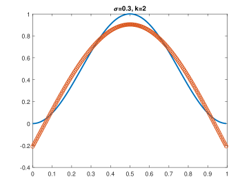
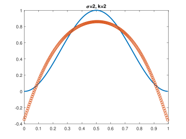
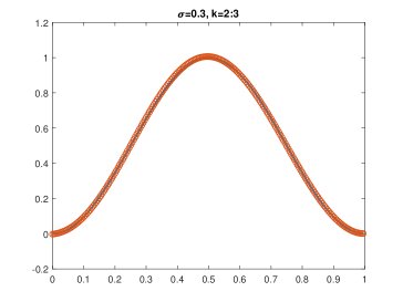
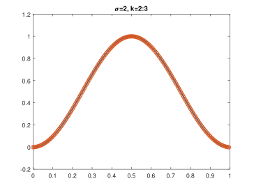
Figure 1. Reconstruction of the strength in Example 1. Solid blue line: exact strength; circled red line: reconstructed strength. For both $\sigma=0.3$ (left column) and $\sigma=2$ (right column), reconstructions based on data at two frequencies $k=2,3$ are better than the ones based on data at a single frequency $k=2$.

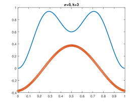
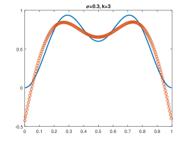
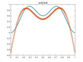
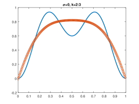
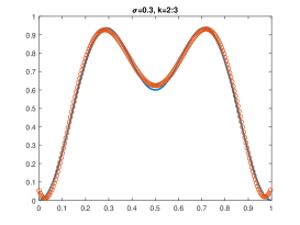
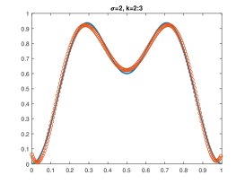
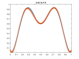
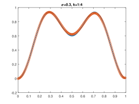
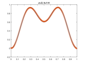
Figure 2. Reconstruction of the strength in Example 2. Solid blue line: exact strength; circled red line: reconstructed strength. For $\sigma=0$ (left column), $\sigma=0.3$ (middle column) and $\sigma=2$ (right column), reconstructions get better when data at more frequencies are used (top: $k=3$; middle: $k=2,3$; bottom: $k=1:4$).

Example 1.

Reconstruct the strength given by

$$\mu(x)=0.5(1-\cos(2\pi x))$$

inside the interval $(0,1)$. Figure 1 plots the reconstructed strength and the exact one based on the modified data $\mathcal{M}(x_{m},k)$ with different attenuation coefficients $\sigma=0.3,2$ at one frequency $k=2$ and two frequencies $k=2,3$. As expected, the better reconstruction can be obtained when data at more frequencies is used. The strength $\mu$ can be properly recovered by data at two frequencies $k=2,3$ since $\mu$ considered in this example contains one low frequency Fourier mode.

Example 2.

Reconstruct the strength given by

$$\mu(x)=0.6-0.3\cos(2\pi x)-0.3\cos(4\pi x)$$

inside the interval $(0,1)$. This example contains two Fourier modes and is a little harder than Example 1. Figure 2 shows the reconstructed strength and the exact one based on the modified data $\mathcal{M}(x_{m},k)$ with different attenuation coefficients $\sigma=0,0.3,2$ at one frequency $k=3$, two frequencies $k=2,3$ and four frequencies $k=1,2,3,4$. Note that if $\sigma=0$, then $\kappa_{\rm i}=0$ and the exponential kernel in (4.2) vanishes. Hence, only the average of the strength $\mu$ can be recovered, and the strength itself can not be uniquely determined based on the data at a single frequency in this case. To reconstruct the strength $\mu$ for the case $\sigma=0$, the multi-frequency data is required. We refer to [6, 21] for the details of inverse random source problem of the one-dimensional Helmholtz equation without attenuation. For $\sigma=0.3,2$, the strength $\mu$ can be properly recovered by using the data at a few frequencies.

Example 3.

Reconstruct the strength given by

$$\mu(x)=0.5e-0.3e^{\cos(4\pi x)}-0.2e^{\cos(6\pi x)}$$

inside the interval $(0,1)$. The strength $\mu$ in this example contains more higher Fourier modes than the two previous examples. Hence, it is expected that the data at more frequencies is required to reconstruct the strength. Figure 3 shows the reconstructed strength and the exact one based on data with $\sigma=0,0.3,2$ at one frequency $k=3$ or more frequencies $k=1,\cdots,8$ and $k=1,\cdots,16$, respectively. For $\sigma=0$, data at a single frequency can hardly recover the strength. For $\sigma=0.3,2$, data at a single frequency could roughly recover the strength, and the reconstructions get better when data at more frequencies is used.

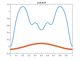
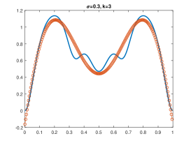
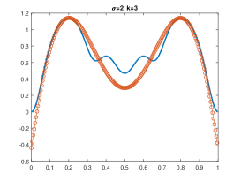
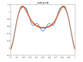
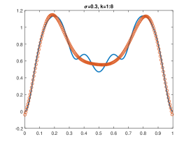
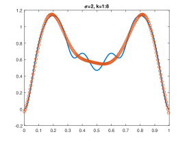
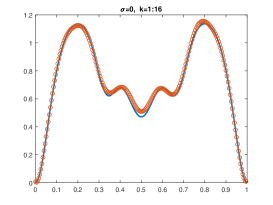
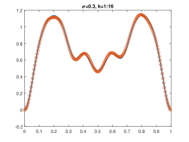
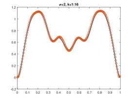
Figure 3. Reconstruction of the strength in Example 3. Solid blue line: exact strength; circled red line: reconstructed strength. For $\sigma=0$ (left column), $\sigma=0.3$ (middle column) and $\sigma=2$ (right column), reconstructions get better when data at more frequencies are used (top: $k=3$; middle: $k=1,\cdots,8$; bottom: $k=1,\cdots,16$), and more frequencies are required to properly reconstruct the strength which contains more higher frequency modes.

6. Conclusion

We have studied an inverse random source scattering problem for the one-dimensional Helmholtz equation with attenuation, which is to reconstruct the strength of the random source. Compared with higher dimensional cases studied in [22], the fundamental solution in the one-dimensional case is smooth, which makes it possible to deal with rougher random sources including the white noise. The strength is shown to be uniquely determined by the variance of the wave field in an open measurement set. The attenuation is essential in the model to get the strength reconstructed point-wisely.

It is open for the recovery of microlocally isotropic random sources for the one-dimensional Helmholtz equation without attenuation as well as the recovery of microlocally isotropic random media for the Helmholtz equation. For the one-dimensional Helmholtz equation without attenuation, only the average of the strength of the microlocally isotropic Gaussian random source over its support could be obtained from on the method presented in this work. For the higher dimensional Helmholtz equation in microlocally isotropic random media, the well-posedness of the direct scattering problem has been studied in [24]; for the inverse problem, however, it is difficult to get the convergence of the Born series generated by the Lippmann–Schwinger equation, which makes it difficult to get an explicit expression of the strength of the random media. Some other mathematical tools need to be explored to deal with these open problems.

References

- [1] R. Adams and J. Fournier, Sobolev Spaces, 2nd ed., Pure and Applied Mathematics 140, Elsevier/Academic Press, Amsterdam, 2003.
- [2] H. Ammari, G. Bao, and J. Fleming, An inverse source problem for Maxwell’s equations in magnetoencephalography, SIAM J. Appl. Math., 62 (2002), pp. 1369–1382.
- [3] G. Bal and A. Tamasan, Inverse source problems in transport equations, SIAM J. Math. Anal., 39 (2007), pp. 57–76.
- [4] G. Bao, C. Chen, and P. Li, Inverse random source scattering problems in several dimensions, SIAM/ASA J. Uncertain. Quantif., 4 (2016), pp. 1263–1287.
- [5] G. Bao, C. Chen, and P. Li, Inverse random source scattering for elastic waves, SIAM J. Numer. Anal., 55 (2017), pp. 2616–2643.
- [6] G. Bao, S.-N. Chow, P. Li, and H. Zhou, An inverse random source problem for the Helmholtz equation, Math. Comp., 83 (2014), pp. 215–233.
- [7] G. Bao, P. Li, and Y. Zhao, Stability for the inverse source problems in elastic and electromagnetic waves, J. Math. Pures Appl., 134 (2020), pp. 122–178.
- [8] G. Bao, J. Lin, and F. Triki, A multi-frequency inverse source problem, J. Differential Equations, 249 (2010), pp. 3443–3465.
- [9] D. Colton and R. Kress, Inverse Acoustic and Electromagnetic Scattering Theory, 3rd ed., Applied Mathematical Sciences 93, Springer, New York, 2013.
- [10] S.-N. Chow, K. Yin, H. Zhou, and A. Behrooz, Solving inverse source problems by the Orthogonal Solution and Kernel Correction Algorithm (OSKCA) with applications in fluorescence tomography, Inverse Probl. Imaging, 8 (2014), pp. 79–102.
- [11] A. Devaney, The inverse problem for random sources, J. Math. Phys., 20 (1979), pp. 1687–1691.
- [12] A. S. Fokas, Y. Kurylev, and V. Marinakis, The unique determination of neuronal currents in the brain via magnetoencephalography, Inverse Problems, 20 (2004), pp. 1067–1082.
- [13] L. Hörmander, The Analysis of Linear Partial Differential Operators I, Classics in Mathematics, Springer-Verlag, Berlin, 2003.
- [14] L. Hörmander, The Analysis of Linear Partial Differential Operators III, Classics in Mathematics, Springer, Berlin, 2007.
- [15] V. Isakov, Inverse Source Problems, Mathematical Surveys and Monographs, 34, American Mathematical Society, Providence, RI, 1990.
- [16] V. Isakov and S. Lu, Increasing stability in the inverse source problem with attenuation and many frequencies, SIAM J. Appl. Math., 78 (2018), pp. 1–18.
- [17] M. Lassas, L. Päivärinta, and E. Saksman, Inverse scattering problem for a two dimensional random potential, Commun. Math. Phys., 279 (2008), pp. 669–703.
- [18] J. Li, T. Helin, and P. Li, Inverse random source problems for time-harmonic acoustic and elastic waves, Commun. Part. Diff. Eqs., to appear.
- [19] J. Li and P. Li, Inverse elastic scattering for a random source, SIAM J. Math. Anal., 51 (2019), pp. 4570–4603.
- [20] J. Li, H. Liu, and S. Ma, Determining a random Schrödinger operator: both potential and source are random, arXiv:1906.01240.
- [21] P. Li, An inverse random source scattering problem in inhomogeneous media, Inverse Problems, 27 (2011), 035004.
- [22] P. Li and X. Wang, Inverse random source scattering for the Helmholtz equation with attenuation, arXiv:1911.11189.
- [23] P. Li and X. Wang, An inverse random source problem for Maxwell’s equations, arXiv:2002.08732.
- [24] P. Li and X. Wang, Regularity of distributional solutions to stochastic acoustic and elastic scattering problems, arXiv:2007.13210.
- [25] A. Lodhia, S. Sheffield, X. Sun, and S. Watson, Fractional Gaussian fields: a survey, Probab. Surv., 13 (2016), pp. 1–56.