Slit-strip Ising boundary conformal field theory 1:
Discrete and continuous function spaces

Abstract.

This is the first in a series of articles about recovering the full algebraic structure of a boundary conformal field theory (CFT) from the scaling limit of the critical Ising model in slit-strip geometry. Here, we introduce spaces of holomorphic functions in continuum domains as well as corresponding spaces of discrete holomorphic functions in lattice domains. We find distinguished sets of functions characterized by their singular behavior in the three infinite directions in the slit-strip domains, and note in particular that natural subsets of these functions span analogues of Hardy spaces. We prove convergence results of the distinguished discrete holomorphic functions to the continuum ones. In the subsequent articles, the discrete holomorphic functions will be used for the calculation of the Ising model fusion coefficients (as well as for the diagonalization of the Ising transfer matrix), and the convergence of the functions is used to prove the convergence of the fusion coefficients. It will also be shown that the vertex operator algebra of the boundary conformal field theory can be recovered from the limit of the fusion coefficients via geometric transformations involving the distinguished continuum functions.

1. Introduction

Conformal invariance results about the Ising model scaling limit

We have witnessed a breakthrough in the mathematically precise understanding of the conformal invariance properties of the critical planar Ising model, following the discrete complex analysis ideas pioneered by Smirnov [Smi06]. The conformal invariance properties arise in the scaling limit of the lattice model, upon zooming out so that the lattice mesh tends to zero.

One facet of the progress has been advances in the random geometry description of the scaling limit. It has been proven that interfaces arising with Dobrushin boundary conditions in both the Ising model and its random cluster model counterpart tend to conformally invariant random curves known as Schramm-Loewner evolutions (SLE)  [Smi10a, ChSm12, CDHKS14]. Generalizations of interface convergence results for boundary conditions other than Dobrushin type have been obtained in [HoKy13, Izy15, Izy17, KeSm19, KeSm17, BDH16, BPW18, PeWu18, Kar19]. The full collection of all interfaces in the Ising model and its random cluster model counterpart tend to processes known as conformal loop ensembles (CLE) [KeSm16, BeHo19].

Instead of the random geometry of interfaces, the physics tradition as well as the constructive quantum field theory tradition place focus on correlation functions. The existence of scaling limits of renormalized Ising model correlation functions, and the conformal covariance of these scaling limits, have been shown for energy [HoSm13, Hon10] and spin [CHI15]. Recently a similar conclusion has been obtained for mixed correlation functions of all primary fields including the spin and energy [CHI21]. It has even been shown that the set of all possible lattice local fields of the Ising model carries a representation of the Virasoro algebra [HKV17], a hallmark of conformal field theories (CFT), and that with generic renormalization local correlation functions of such fields have conformally covariant limits  [GHP19]. Building on the correlation function results, it has furthermore been proven that the collection of Ising spins viewed as a random field converges to a conformally covariant scaling limit [CGN15, CGN16].

The 100 year history of the Ising model contains a wealth of ingenious mathematical ideas that have enabled rigorous results, including transfer matrix methods [KrWa41, Ons44, Yan52] and their fermionic formulations [Kau49, SML64] and Toeplitz determinants [MPW63, Wu66, FiHa69], Kac-Ward matrices [KaWa52], dimer representations [Kas63, Fis66], discrete complex analysis [KaCe71, Mer01], commuting families of transfer matrices [StMi72], Yang-Baxter equations [BaEn78], non-linear differential equations (particularly Painlevé type) and difference equations  [WMTB76, Per80, JiMi80], and bosonization [Dub11]; for more on the various mathematical developments see, e.g., [McWu73, Bax82, Pal07] and [DIK13, CCK17]. The recent breakthrough mathematical progress on the conformal invariance of both random geometry and correlation functions of the Ising model, however, has been enabled mainly by novel notions of discrete complex analysis that apply particularly well to the Ising model: s-holomorphicity and specific Riemann boundary value problems [Smi10a, ChSm11, ChSm12].

The conformal field theory picture

The prediction of conformal invariance was made in theoretical physics research in the 1980’s, in a research field titled conformal field theory (CFT). Physicists predicted that, very generally, models of two-dimensional statistical physics at their critical points of continuous phase transitions should, in the scaling limit, be described by field theories with conformal symmetry [BPZ84b]. Such conformal field theories turn out to be algebraically very stringently constrained [BPZ84a] — in mathematical terms their chiral symmetry algebras are vertex operator algebras (VOA) [FLM88, Kac97, LeLi04, Hua12]. This prediction and the associated algebraic structure leads to absolutely remarkable, specific, exact predictions about the statistical physics models — including values of critical exponents, formulas for scaling limit correlation functions, modular invariance of renormalized scaling limit partition functions on tori, etc., see, e.g. [DMS97, Mus09].

The square lattice Ising model is an archetype of such statistical physics models, and known results about it lend very strong support to the predicted general picture. But although there is thus virtually no doubt that the conformal field theory picture for the scaling limit of the Ising model is correct in an exact sense without approximations, there is still no mathematical result establishing a complete conformal field theory as the scaling limit of the critical Ising model, and one even struggles to find a precisely stated mathematical conjecture about it in the literature!

The general goal of this series of articles is to remedy this situation by showing that the full algebraic structure of the conformal field theory generally conjectured to describe the scaling limit of the Ising model is indeed recovered in the scaling limit. More precisely, the combination of results proven in this series establishes that the fusion coefficients of the Ising model with locally monochromatic boundary conditions in slit-strip geometry (defined in [AKP21] as renormalized limits of boundary correlation functions in lattice slit-strips) converge in the scaling limit to the structure constants of the vertex operator algebra of the fermionic Ising boundary conformal field theory.

Slit-strip geometry and boundary conformal field theory

In this series of articles we consider the Ising model in lattice approximations of the strip and slit-strip geometries illustrated in Figures 2.1. Likewise, we extensively use spaces of holomorphic functions in the strip and the slit-strip, as well as discrete holomorphic functions in their lattice approximations. Let us briefly explain the role that these geometries play in boundary conformal field theory.

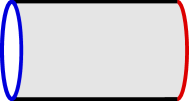
(a) Cylinder surface.

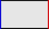
(b) Strip surface (truncated).

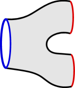
(c) Pair-of-pants surface.

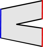
(d) Slit-strip surface (truncated).

Figure 1.1. The (truncated) strip and (truncated) slit-strip surfaces have the same role in boundary CFT as the cylinder and pair-of-pants surfaces have in bulk CFT.

The rough idea is that the strip and the slit-strip are for boundary conformal field theory what the cylinder (or annulus) and the pair-of-pants Riemann surfaces are for bulk conformal field theory. Let us begin with the more familiar setup of bulk conformal field theory. The role of geometry is most transparent in Segal’s axiomatization of conformal field theories [Seg88, Seg04], in which a CFT is defined as a (projective) functor — subject to certain axioms — from the category whose morphisms are bordered Riemann surfaces with parametrized boundary components to the category whose morphisms are trace-class operators between tensor products of a given Hilbert space. Segal’s approach is clearly motivated by the transfer matrix formalism in statistical mechanics: the operators associated to cylider surfaces (of different moduli) form a semigroup which is thought of as the scaling limit of the semigroup generated by the transfer matrix itself.

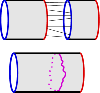
(a) Sewing together cylinders.

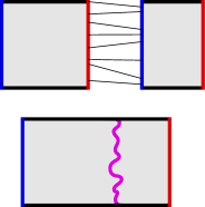
(b) Sewing together rectangles.

Figure 1.2. The sewing together of cylinders in bulk CFT and the sewing together of truncated strips (i.e., rectangles) in boundary CFT give rise to semigroups that correspond to the scaling limits of the transfer matrices.

Sewing together bordered Riemann surfaces along (parametrized) boundary components is the composition in the category. Cylinder surfaces alone can only be sewn with each other to form cylinders (sew together two cylinders) as in Figure 1.2(a) or tori (sew together the two ends of a cylinder). On the other hand, the pair-of-pants surfaces can be sewn together as in Figure 1.3 to form surfaces of arbitrary genus, and in this sense they are the building block of all Riemann surfaces. The use of the term vertex operator (and the symbol $Y$ used for it) originates from the picture of the pair-of pants surface (a vertex diagram in string theory) and the operator that is associated with this surface.

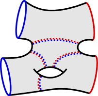
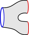
Figure 1.3. Sewing many pair-of-pants can produce arbitrary genus surfaces.

It is a natural change in the point of view [Hua12, RSS17] to equip the bordered Riemann surfaces with tubes (cylinders infinitely extended in one direction) attached to the boundary components so that the surfaces become punctured surfaces: the punctures correspond to the infinite extremities of the tubes (and thus there is one for each boundary component of the original bordered Riemann surface) and they become equipped with a choice of local coordinates. With this point of view, cylinders correspond to the Riemann sphere with two punctures, and the pair-of-pants corresponds to the the Riemann sphere with three punctures.

A rectangle, or equivalently a truncated strip, is the natural counterpart in boundary conformal field theory to a cylinder of finite modulus in bulk conformal field theory, whereas the doubly infinite strip is the counterpart of the cylinder with tubes attached to each end, i.e., the twice-punctured sphere. The transfer matrix is, indeed, simplest to use for calculations in rectangles and strips. Along with the main result of this series, we will of course also verify the familiar statement that the scaling limits of powers of transfer matrices form the semigroup generated by the energy operator $L_{0}$ in the vertex operator algebra, in agreement with the interpretation in Segal’s formulation.

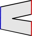
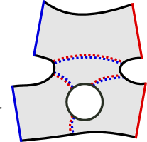
Figure 1.4. Sewing many truncated slit-strips can produce arbitrary multiply connected domains.

A truncated slit-strip is the natural counterpart in boundary conformal field theory for a pair-of-pants surface in bulk conformal field theory, whereas the infinite slit-strip (with three infinite extremities) is the counterpart of the pair-of-pants with tubes attached to each end, i.e., the thrice-punctured sphere. By sewing together boundary intervals of (surfaces conformally equivalent to) truncated slit-strips, it is possible to build general multiply connected planar domains with boundaries as in Figure 1.4. In this sense the slit-strip geometry is the building block of general domains in boundary conformal field theory in exactly the same way that the pair-of-pants surface is in bulk conformal field theory.

Our main result that the fusion coefficients of the Ising model with locally monochromatic boundary conditions in the lattice slit-strip tend, in the scaling limit, to the structure constants of the vertex operator algebra, therefore recover the clear boundary conformal field theory analogue of the role that vertex operators have in bulk conformal field theory as operators associated with the pair-of-pants geometry.

Overview of the series

This series of articles is divided into three parts.

Part 1: Discrete and continuous function spaces:

This first part concerns the function spaces needed in the analysis of the scaling limit of the Ising model fusion coefficients. We will consider spaces of holomorphic solutions to a Riemann boundary value problem in the strip and the slit-strip, as well as their discretized analogues: spaces of s-holomorphic solutions to a Riemann boundary value problem in a lattice strip and a lattice slit-strip. We will, in particular, study the restrictions of such functions to a cross-section of the strip or the slit-strip — much like in Segal’s CFT one would view cross-sections of surfaces as carrying physical states in the Hilbert space, which are then acted on by the operators associated to Riemann surfaces lying between different cross-sections. The Riemann boundary values (and s-holomorphicity) are real-linear conditions, and the function spaces here will all be real vector spaces. They will have the natural Hilbert space structure coming from square integrability of the functions on cross-sections. We will find and concretely describe distinguished bases of functions, which have prescribed singularities in one of the infinite extremities and which are regular in the other two. We prove the convergence of the distinguished functions on the lattices to the distinguished continuum functions, and the convergence of all corresponding inner products. The distinguished discrete functions in both the lattice strip and the lattice slit-strip will be crucially used in the calculations with the Ising model in the second part [AKP21]. The distinguished continuum functions in the slit-strip will be used as a more natural basis for calculations with the vertex operator algebra in the third part [KPR20].

Part 2: Scaling limits of fusion coefficients:

The second part of this series [AKP21] will focus on the Ising model itself, in the lattice strip and the lattice slit-strip and with locally monochromatic boundary conditions. It will be shown that there is a way to diagonalize the transfer matrices associated with the strip and the slit-strip using Clifford algebra valued discrete one-forms built from one set of distinguished discrete functions in the present article, and that s-holomorphicity and Riemann boundary values underlie the possibility to perform contour deformations in the integrals of these one-forms. The contour deformations are clearly analogous to boundary conformal field theory, and using them with the other set of distinguished discrete functions of the present article, we derive a recursive characterization of the fusion coefficients of the Ising model. The recursion involves inner products of the distinguished discrete functions, and by the present results on their convergence, we will be able to derive the convergence of the fusion coefficients in the scaling limit.

Part 3: The vertex operator algebra in the scaling limit:

In the third part of this series [KPR20] we arrive at the main statement: from the scaling limits of the fusion coefficients one can recover the structure constants of the vertex operator algebra of the fermionic conformal field theory that has been claimed to describe the Ising model, and conversely from the structure constants one can recover the scaling limits of the fusion coefficients. The recovery involves only changes of bases related to the choice of natural local coordinates at the three infinite extremities of the slit-strip; which again naturally involve the distinguished continuum functions of the present article.

Together, the series provides a fully rigorously worked out model case of a mathematically precise statement about the emergence of the full algebraic structure of a boundary conformal field theory in the scaling limit of a lattice model of statistical mechanics. Given the broad conjectured validity of the conformal field theory picture, this should be viewed as the prototype of a precise conjecture to be formulated about many other models. Some of our steps are inevitably specific to the Ising model (particularly the role of s-holomorphicity and Riemann boundary values), but certain steps could even offer technical insights into the cases of other models.

Organization of this article

This first article of the series is organized as follows.

Section 2:

We define the continuum function spaces and find the distinguished holomorphic solutions to the Riemann boundary value problems in the strip and the slit-strip. In the case of the strip, the distinguished functions are eigenfunctions of vertical translations, and their restrictions to horizontal cross-sections are simply certain Fourier modes with a quarter-of-a-full-turn phase difference between the two boundaries. In the slit-strip, the distinguished functions are constructed as linear combinations of pull-backs of certain monomial functions from the upper half-plane.

Section 3:

We define the discrete function spaces and find the distinguished s-holomorphic solutions to the Riemann boundary value problems in the lattice strip and the lattice slit-strip. The distinguished functions in the lattice slit-strip are again vertical translation eigenfunctions, whose restrictions to a cross-section turn out to be combinations of two discrete Fourier modes with opposite frequencies. The qualitative properties of the spectrum of the vertical translations of s-holomorphic solutions to the Riemann boundary value problem in the strip were observed in [HKZ14], but for our purposes we need both the spectrum and the eigenfuctions explicitly. This explicit calculation is essentially equivalent to the diagonalization of the induced rotation of the transfer matrix on the space of Clifford generators [Pal07], but we find the vertical translation eigenfunction problem for discrete holomorphic functions conceptually simpler, and we provide the details of the derivation also so that the series constitutes a self-contained proof of the main result. The distinguished functions in the lattice slit-strip can be constructed based on the invertibility of a finite-dimensional linear system of subspace projection equations.

Section 4:

The final section addresses the convergence of the distinguished discrete functions to the continuum ones. Having calculated the vertical translation eigenfunctions in the lattice strip explicitly, their convergence becomes a matter of straightforward inspection. The remaining results rely on the “imaginary part of the integral of the square” technique [Smi06, ChSm11, ChSm12]. We first of all use it to prove the invertibility of the linear system of subspace projections from the previous section. Moreover, the resulting regularity theory for s-holomorphic functions is used to prove the convergence of the distinguished discrete functions in the slit-strip.

Novelty

We do not claim essential novelty in any of the results concerning the strip geometry — this case is included mainly for coherent formulation of the whole: the definitions are needed in any case, and proofs are provided for self-containedness. All of our calculations in the lattice strip are fully explicit and in essence equivalent to the calculations needed to diagonalize the transfer matrix of the Ising model with locally monochromatic boundary conditions. The well known diagonalization of this transfer matrix [AbMa73, Pal07] in particular allows one to conclude without difficulty that the suitable powers of the transfer matrix converge to the exponentials of the energy operator $L_{0}$ in the vertex operator algebra of the fermionic Ising CFT, for example by realizing the VOA as an inductive limit of transfer state spaces.

Instead, the novelty of our work pertains almost exclusively to the slit-strip geometry. Key objects for us are the distinguished functions in the lattice slit-strip, whose asymptotics in one of the extremities matches the behavior of the explicit strip functions. Such globally defined discrete holomorphic functions are analogous to objects needed in Segal’s CFT for vertex operators; not merely the semigroup generated by the energy operator $L_{0}$. The fact that such globally defined s-holomorphic functions exist at all is crucial to our later contour deformation arguments, and their convergence is at the heart of the convergence of the Ising model fusion coefficients. For both of these, recently developed specific techniques of discrete complex analysis [Smi06, Smi10a, ChSm11, ChSm12] are indispensable. And it is precisely thus established convergence and recursion properties of the Ising model fusion coefficients which allow us to recover the vertex operator algebra in the scaling limit.

2. Continuum function spaces and decompositions

In this section, we introduce the function spaces which play a crucial role in our analysis of the continuum limit of the Ising model fusion coefficients. A key notion are certain Riemann boundary values for holomorphic functions [Smi06]. The notion has found some use in functional analysis [HoPh13], but it is the analogous notion in the lattice setup that has turned out particularly fruitful for the study of the Ising model [Smi10b, Che18]. The straightforward continuum problem considered in the current section provides an instructive blueprint for what to expect of the lattice discretizations of Section 3.

For our purposes, holomorphic functions with Riemann boundary values will be studied in two different geometries: the infinite strip ${\mathbb{S}}$ and the infinite slit-strip ${\mathbb{S}}_{\mathrm{slit}}$ of Figure 2.1. In the spirit of Segal’s geometric formulation of conformal field theories [Seg88, Seg04], we focus in particular on the restrictions of such functions to a crosscut of the strip or the slit-strip. In both cases, the crosscut is basically an interval, and the appropriate function space is a space of square-integrable complex valued functions on the crosscut interval. This space of complex valued functions is made into a real Hilbert space, because the Riemann boundary values are a real-linear condition. An obvious difference to Segal’s formulation is that we consider geometries with boundaries, analogous to open-string string theory rather than the more common closed-string version for which Segal’s formulation is directly suitable. Correspondingly the cross sections are not (disjoint unions of) circles as in Segal’s formulation, but rather (disjoint unions of) intervals.

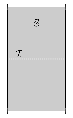
(a) The infinite vertical strip ${\mathbb{S}}$ and its horizontal cross-section $\mathcal{I}$.

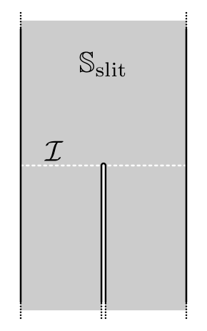
(b) The infinite slit-strip ${\mathbb{S}}_{\mathrm{slit}}$ and its horizontal cross-section $\mathcal{I}$.

Figure 2.1. The strip and slit-strip domains.

In Section 2.1 we define the Riemann boundary values, and introduce the appropriate function spaces for the strip and the slit-strip geometries. In Section 2.2 we introduce the basis of the function space corresponding to vertical translation eigenfunctions in the strip. These continuum functions are just Fourier modes with a quarter-integer phase difference between boundaries, but their discrete analogues will be a key to the diagonalization of the Ising transfer matrix. In Section 2.3 we introduce analogous functions in the slit-strip, defined locally near each of the three extremities of the slit-strip, as well as globally defined functions which have prescribed singularities at the three extremities. The latter will feature naturally in expressions for VOA matrix elements.

2.1. Functions in the strip and the slit-strip

Riemann boundary values for holomorphic functions

Let $\Omega\subset\mathbb{C}$ be a domain (open, connected subset). Suppose that $x_{0}\in\partial\Omega$ is a boundary point of the domain (more precisely a prime end) such that locally near $x_{0}$ the boundary $\partial\Omega$ is a smooth curve, and let $\tau(x_{0})$ be a unit complex number representing the direction of the counterclockwise oriented tangent to the boundary at $x_{0}$. A holomorphic function $F:\Omega\to\mathbb{C}$ which continuously extends to $x_{0}$ has Riemann boundary value at $x_{0}$ if

(2.1) $$F(x_{0})\in\mathbbm{i}\,\tau(x_{0})^{-1/2}\,\mathbb{R}.$$

The strip and the slit-strip

The two domains of interest to us will be the unit width vertical strip

(2.2) $${\mathbb{S}}:=\left\{z\in\mathbb{C}\;\bigg{|}\;-\frac{1}{2}<\Re\mathfrak{e}(z)<\frac{1}{2}\right\}$$

and the slit-strip

(2.3) $${\mathbb{S}}_{\mathrm{slit}}:={\mathbb{S}}\setminus\left\{\mathbbm{i}y\;\big{|}\;y\leq 0\right\}.$$

These domains are illustrated in Figure 2.1.

According to definition (2.1), a holomorphic function $F\colon{\mathbb{S}}\to\mathbb{C}$ in the strip has Riemann boundary values if for all $y\in\mathbb{R}$ we have

(2.4) $$F\Big{(}\frac{-1}{2}+\mathbbm{i}y\Big{)}\in e^{-\mathbbm{i}\pi/4}\,\mathbb{R}\qquad\text{ and }\qquad F\Big{(}\frac{+1}{2}+\mathbbm{i}y\Big{)}\in e^{+\mathbbm{i}\pi/4}\,\mathbb{R}.$$

For a holomorphic function $F\colon{\mathbb{S}}_{\mathrm{slit}}\to\mathbb{C}$ to have Riemann boundary values in the slit-strip, in addition to the above it is required that for any $y<0$, the left and right limits on the slit part of the boundary satisfy

(2.5) $$F\big{(}0^{-}+\mathbbm{i}y\big{)}\in e^{+\mathbbm{i}\pi/4}\,\mathbb{R}\qquad\text{ and }\qquad F\big{(}0^{+}+\mathbbm{i}y\big{)}\in e^{-\mathbbm{i}\pi/4}\,\mathbb{R}.$$

The horizontal cross-section

We study functions on the strip ${\mathbb{S}}$ and the slit-strip ${\mathbb{S}}_{\mathrm{slit}}$ domains through their restrictions to the horizontal cross-section at zero imaginary part

(2.6) $$\mathcal{I}:=\left[-\frac{1}{2},\frac{1}{2}\right],$$

and therefore consider appropriate spaces of complex valued functions on this interval. For this purpose, we use the real Hilbert space

(2.7) $$\mathscr{L}^{2}:=L^{2}_{\mathbb{R}}(\mathcal{I},\mathbb{C}),$$

of square-integrable complex valued functions on the cross section. The square-integrability requirement can be seen as imposing the Riemann bounday value also at the tip of the slit, in an appropriate (conformal) sense. The norm $\|f\|$ of $f\in\mathscr{L}^{2}$ is obtained from

$$\|f\|^{2}=\int_{-\frac{1}{2}}^{\frac{1}{2}}|f(x)|^{2}\;\mathrm{d}x,$$

as usual, but we emphasize that the inner product takes the form

(2.8) $$\langle f,g\rangle=\; \int_{-\frac{1}{2}}^{\frac{1}{2}}\Big{(}\Re\mathfrak{e}\big{(}f(x)\big{)}\,\Re\mathfrak{e}\big{(}g(x)\big{)}+\Im\mathfrak{m}\big{(}f(x)\big{)}\,\Im\mathfrak{m}\big{(}g(x)\big{)}\Big{)}\;\mathrm{d}x$$

$$=\; \int_{-\frac{1}{2}}^{\frac{1}{2}}\Re\mathfrak{e}\Big{(}f(x)\,\overline{g(x)}\Big{)}\;\mathrm{d}x,$$

since we view $\mathscr{L}^{2}$ as a Hilbert space over $\mathbb{R}$, not $\mathbb{C}$.

2.2. Decomposition into vertical translation eigenfunctions

First, consider functions in the vertical strip ${\mathbb{S}}$. We look for holomorphic functions $F\colon{\mathbb{S}}\to\mathbb{C}$ with Riemann boundary values (2.4), which are furthermore eigenfunctions for vertical translations, i.e.,

(2.9) $$F(z+\mathbbm{i}h)=\Lambda(h)F(z)\qquad\text{ for all $z\in{\mathbb{S}}$ and $h\in\mathbb{R}$.}$$

The vertical translation eigenfunction property (2.9) is clearly only possible if $\Lambda(h)=e^{ph}$ for some $p$, and it also implies that the function must factorize as ${F(x+\mathbbm{i}y)=f(x)\,e^{py}}$. Cauchy-Riemann equations then amount to $f^{\prime}(x)+\mathbbm{i}pf(x)=0$, which yields $f(x)\propto e^{-\mathbbm{i}px}$. The Riemann-boundary values (2.4) in turn can be satisfied only if $e^{\mathbbm{i}p}=f(\frac{-1}{2})/f(\frac{+1}{2})\in\mathbbm{i}\mathbb{R}$, i.e., $p\in\pi\mathbb{Z}+\frac{\pi}{2}$. The functions of interest to us are therefore basically the analytic continuations of quarter-integer Fourier modes on the cross-section $\mathcal{I}$ (the argument makes one quarter-turn plus any number of half-turns from one end of the interval $\mathcal{I}$ to the other).

For indexing the Fourier modes (as well as the fermion modes in the vertex operator algebra later on), we use the sets of positive half-integers and of all half-integers denoted in what follows by

(2.10) $$\mathcal{K}:=\; \big{[}0,+\infty\big{)}\cap\Big{(}\mathbb{Z}+\frac{1}{2}\Big{)}=\left\{\frac{1}{2},\frac{3}{2},\frac{5}{2},\ldots\right\},$$

$$\pm\mathcal{K}:=\; \mathcal{K}\cup(-\mathcal{K})=\mathbb{Z}+\frac{1}{2}=\left\{\pm\frac{1}{2},\pm\frac{3}{2},\ldots\right\}.$$

Then, for $k\in\pm\mathcal{K}$, we define the function

(2.11) $$E_{k}(x+\mathbbm{i}y):=C_{k}\;\exp\big{(}-\mathbbm{i}\pi kx+\pi ky\big{)},\qquad\text{ for }x+\mathbbm{i}y\in{\mathbb{S}},$$

and its restriction to the cross section

(2.12) $$e_{k}(x):=C_{k}\;e^{-\mathbbm{i}\pi kx}\qquad\text{ for }x\in\mathcal{I},$$

where the normalization constant is chosen as

(2.13) $$C_{k}:=\; e^{\mathbbm{i}\pi(-k/2-1/4)}$$

to ensure $E_{k}\big{(}\frac{-1}{2}+\mathbbm{i}y\big{)}\in e^{-\mathbbm{i}\pi/4}\,\mathbb{R}_{+}$ and $\|e_{k}\|=1$. These quarter-integer Fourier modes (2.12) are illustrated in Figure 2.2. Let us start by checking that they form an orthonormal basis of our function space $\mathscr{L}^{2}$.

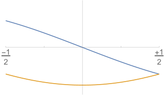
(a) The Fourier mode $e_{k}$ for $k=1/2$.

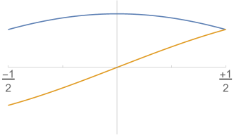
(b) The Fourier mode $e_{k}$ for $k=-1/2$.

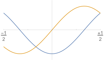
(c) The Fourier mode $e_{k}$ for $k=3/2$.

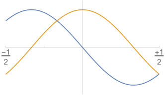
(d) The Fourier mode $e_{k}$ for $k=-3/2$.

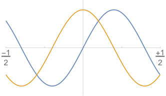
(e) The Fourier mode $e_{k}$ for $k=5/2$.

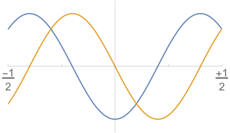
(f) The Fourier mode $e_{k}$ for $k=-5/2$.

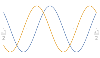
(g) The Fourier mode $e_{k}$ for $k=7/2$.

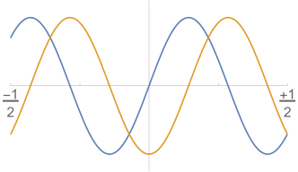
(h) The Fourier mode $e_{k}$ for $k=-7/2$.

Figure 2.2. Real and imaginary parts (blue and orange) of the restrictions $e_{k}$ of the vertical translation eigenfunctions $E_{k}$ to the cross section $\mathcal{I}=[\frac{-1}{2},\frac{1}{2}]$. Riemann boundary conditions (2.4) fix the ratio of the real and imaginary parts at the two endpoints, and our normalization (2.13) fixes the phase at the left endpoint.

Proposition 2.1.

The collection $(e_{k})_{k\in\pm\mathcal{K}}$ is an orthonormal basis for the real Hilbert space $\mathscr{L}^{2}$. In particular, for $k,k^{\prime}\in\pm\mathcal{K}$ we have

(2.14) $$\langle e_{k},e_{k^{\prime}}\rangle=\delta_{k,k^{\prime}}.$$

Proof.

Orthonormality (2.14) is shown by a routine trigonometric integral. It thus remains to show completeness of the collection $(e_{k})_{k\in\pm\mathcal{K}}$.

Given $f\in\mathscr{L}^{2}$, a square-integrable complex valued function on the interval $[-1/2,+1/2]$ of length $1$, define a period $4$ extension of $f$ to $\mathbb{R}$ as follows. First extend $f$ to $[-1/2,+3/2]$ by $f(1-x)=\mathbbm{i}\,\overline{f(x)}$, and then extend to $\mathbb{R}$ by the antiperiodicity condition $f(x+2)=-f(x)$. By ordinary Fourier series, we can write this extended square-integrable function on $[-2,2]$ as $f(x)=\sum_{n\in\mathbb{Z}}c_{n}\,e^{-\mathbbm{i}nx\pi/2}$, with some complex coefficients $c_{n}\in\mathbb{C}$. It follows from antiperiodicity that the even coefficients vanish, $c_{2m}=0$ for all $m\in\mathbb{Z}$. From the reflection property $f(1-x)=\mathbbm{i}\,\overline{f(x)}$ it follows that the odd coefficients satisfy $c_{2k}+\mathbbm{i}^{2k-1}\,\overline{c_{2k}}=0$ for all $k\in\pm\mathcal{K}$, i.e., that $c_{2k}$ lies on the line $\mathbb{R}C_{k}$ in the complex plane. The terms in this Fourier series are therefore real multiples of the basis functions $e_{k}$, $k\in\pm\mathcal{K}$. Completeness follows. ∎

Remark 2.2.

The functions obtained by imaginary multiplication $x\mapsto\mathbbm{i}\,e_{k}(x)$, and complex conjugation $x\mapsto\overline{e_{k}(x)}$ are obviously also square-integrable, and related by $\overline{e_{k}(x)}=\mathbbm{i}\,e_{-k}(x)$. Note that the expansions of both of these in the basis $(e_{k})_{k\in\pm\mathcal{K}}$ of  $\mathscr{L}^{2}$ (with real coefficients!) contain infinitely many terms. The combination of the two operations, however, amounts to simply changing the sign of the mode, $\overline{\mathbbm{i}\,e_{k}(x)}=e_{-k}(x)$, as is evident also in Figure 2.2.

The positive and negative modes form a splitting of the Hilbert space into two orthogonally complementary subspaces

$$\mathscr{L}^{2}=\; \mathscr{L}^{2}_{\mathrm{T};\mathrm{pole}}\oplus\mathscr{L}^{2}_{\mathrm{T};\mathrm{zero}},$$

where

(2.15) $$\mathscr{L}^{2}_{\mathrm{T};\mathrm{pole}}:=\; \overline{\mathrm{span}_{\mathbb{R}}\left\{e_{k}\;\big{|}\;k>0\right\}} \mathscr{L}^{2}_{\mathrm{T};\mathrm{zero}}:=\; \overline{\mathrm{span}_{\mathbb{R}}\left\{e_{k}\;\big{|}\;k<0\right\}}.$$

We denote the orthogonal projections to these two subspaces by

$$\Pi_{\mathrm{T};\mathrm{pole}}\colon\; \mathscr{L}^{2}\to\mathscr{L}^{2}_{\mathrm{T};\mathrm{pole}} \Pi_{\mathrm{T};\mathrm{pole}}(e_{k})=\begin{cases}0&\text{ if $k<0$}\\ e_{k}&\text{ if $k>0$}\end{cases}$$

$$\Pi_{\mathrm{T};\mathrm{zero}}\colon\; \mathscr{L}^{2}\to\mathscr{L}^{2}_{\mathrm{T};\mathrm{zero}} \Pi_{\mathrm{T};\mathrm{zero}}(e_{k})=\begin{cases}e_{k}&\text{ if $k<0$}\\ 0&\text{ if $k>0$}.\end{cases}$$

2.3. Decomposition of holomorphic functions in the slit-strip

With particularly the slit-strip ${\mathbb{S}}_{\mathrm{slit}}$ in mind we also use functions defined in the left and right halves of the strip,

(2.16) $${\mathbb{S}}^{\mathrm{L}}:= \left\{z\in\mathbb{C}\;\bigg{|}\;\frac{-1}{2}<\Re\mathfrak{e}(z)<0\right\}, {\mathbb{S}}^{\mathrm{R}}:= \left\{z\in\mathbb{C}\;\bigg{|}\;0<\Re\mathfrak{e}(z)<\frac{+1}{2}\right\},$$

and their restrictions to left and right halves of the cross sections

(2.17) $$\mathcal{I}^{\mathrm{L}}:=\; \Big{[}\frac{-1}{2},0\Big{]}, \mathcal{I}^{\mathrm{R}}:=\; \Big{[}0,\frac{+1}{2}\Big{]}.$$

The space of square-integrable functions has an orthogonal decomposition into functions with support in the left and right halves,

$$\mathscr{L}^{2}=\mathscr{L}^{2}_{\mathrm{L}}\oplus\mathscr{L}^{2}_{\mathrm{R}},$$

where we can interpret (modulo extension by zero to the other half)

$$\mathscr{L}^{2}_{\mathrm{L}}=\; L^{2}_{\mathbb{R}}(\mathcal{I}^{\mathrm{L}},\mathbb{C}), \mathscr{L}^{2}_{\mathrm{R}}=\; L^{2}_{\mathbb{R}}(\mathcal{I}^{\mathrm{R}},\mathbb{C}).$$

The quarter-integer Fourier modes for the left and right halves are defined by

(2.18) $$E^{\mathrm{L}}_{k}(x+\mathbbm{i}y)=\; C^{\mathrm{L}}_{k}\;\exp\big{(}-\mathbbm{i}2\pi kx+2\pi ky\big{)}, e^{\mathrm{L}}_{k}(x)=\; C^{\mathrm{L}}_{k}\,e^{-\mathbbm{i}2\pi kx}$$

(2.19) $$E^{\mathrm{R}}_{k}(x+\mathbbm{i}y)=\; C^{\mathrm{R}}_{k}\;\exp\big{(}-\mathbbm{i}2\pi kx+2\pi ky\big{)}, e^{\mathrm{R}}_{k}(x)=\; C^{\mathrm{R}}_{k}\,e^{-\mathbbm{i}2\pi kx},$$

for $k\in\pm\mathcal{K}$, where we choose $C^{\mathrm{L}}_{k}=\sqrt{2}\,e^{\mathbbm{i}\pi(-k-1/4)}$ and $C^{\mathrm{R}}_{k}=\sqrt{2}\,e^{-\mathbbm{i}\pi/4}$ to ensure ${E^{\mathrm{L}}_{k}\big{(}\frac{-1}{2}+\mathbbm{i}y\big{)}}\in e^{-\mathbbm{i}\pi/4}\,\mathbb{R}_{+}$ and $\|e^{\mathrm{L}}_{k}\|=1$, and ${E^{\mathrm{R}}_{k}\big{(}0+\mathbbm{i}y\big{)}}\in e^{-\mathbbm{i}\pi/4}\,\mathbb{R}_{+}$ and $\|e^{\mathrm{R}}_{k}\|=1$, respectively.

The following orthonormal basis properties follow easily from Proposition 2.1 again.

Proposition 2.3.

The collections $(e^{\mathrm{L}}_{k})_{k\in\pm\mathcal{K}}$ and $(e^{\mathrm{R}}_{k})_{k\in\pm\mathcal{K}}$ are orthonormal bases for the real Hilbert spaces $\mathscr{L}^{2}_{\mathrm{L}}$ and $\mathscr{L}^{2}_{\mathrm{R}}$, respectively. These two collections combined form a basis for the real Hilbert space $\mathscr{L}^{2}=\mathscr{L}^{2}_{\mathrm{L}}\oplus\mathscr{L}^{2}_{\mathrm{R}}$.

We can further split the functions with support on one of the two halves to those with negative or positive modes in the corresponding half, i.e., write

$$\mathscr{L}^{2}_{\mathrm{L}}=\; \mathscr{L}^{2}_{\mathrm{L};\mathrm{pole}}\oplus\mathscr{L}^{2}_{\mathrm{L};\mathrm{zero}}, \mathscr{L}^{2}_{\mathrm{R}}=\; \mathscr{L}^{2}_{\mathrm{R};\mathrm{pole}}\oplus\mathscr{L}^{2}_{\mathrm{R};\mathrm{zero}},$$

where

(2.20) $$\mathscr{L}^{2}_{\mathrm{L};\mathrm{pole}}:=\; \overline{\mathrm{span}_{\mathbb{R}}\left\{e^{\mathrm{L}}_{k}\;\big{|}\;k<0\right\}} \mathscr{L}^{2}_{\mathrm{R};\mathrm{pole}}:=\; \overline{\mathrm{span}_{\mathbb{R}}\left\{e^{\mathrm{R}}_{k}\;\big{|}\;k<0\right\}}$$

$$\mathscr{L}^{2}_{\mathrm{L};\mathrm{zero}}:=\; \overline{\mathrm{span}_{\mathbb{R}}\left\{e^{\mathrm{L}}_{k}\;\big{|}\;k>0\right\}} \mathscr{L}^{2}_{\mathrm{R};\mathrm{zero}}:=\; \overline{\mathrm{span}_{\mathbb{R}}\left\{e^{\mathrm{R}}_{k}\;\big{|}\;k>0\right\}}.$$

Remark 2.4.

In (2.15), the poles corresponded to positive indices $k>0$ and zeros to negative indices $k<0$; the former Fourier modes are tending to infinity in the top extremity of the strip, and the latter to zero. Here in (2.20) we instead care about the asymptotics in the left and right downwards extremities of the slit-strip, where it is the modes with negative indices that tend to infinity and modes with positive indices that tend to zero — hence the opposite convention for the correspondence between labels and indices.

We have thus introduced two decompositions of the function space $\mathscr{L}^{2}$:

(2.21) $$\mathscr{L}^{2}=\; \mathscr{L}^{2}_{\mathrm{T};\mathrm{pole}}\oplus\mathscr{L}^{2}_{\mathrm{T};\mathrm{zero}},$$

and

(2.22) $$\mathscr{L}^{2}=\; \mathscr{L}^{2}_{\mathrm{L};\mathrm{pole}}\oplus\mathscr{L}^{2}_{\mathrm{L};\mathrm{zero}}\oplus\mathscr{L}^{2}_{\mathrm{R};\mathrm{pole}}\oplus\mathscr{L}^{2}_{\mathrm{R};\mathrm{zero}}.$$

The orthogonal projections to the two subspaces in decomposition (2.21) are denoted by $\Pi_{\mathrm{T};\mathrm{pole}}\colon\mathscr{L}^{2}\to\mathscr{L}^{2}_{\mathrm{T};\mathrm{pole}}$ and $\Pi_{\mathrm{T};\mathrm{zero}}\colon\mathscr{L}^{2}\to\mathscr{L}^{2}_{\mathrm{T};\mathrm{zero}}$. We denote the orthogonal projections onto the four subspaces in decomposition (2.22) by

$$\Pi_{\mathrm{L};\mathrm{pole}}\colon\; \mathscr{L}^{2}\to\mathscr{L}^{2}_{\mathrm{L};\mathrm{pole}}, \Pi_{\mathrm{R};\mathrm{pole}}\colon\; \mathscr{L}^{2}\to\mathscr{L}^{2}_{\mathrm{R};\mathrm{pole}},$$

$$\Pi_{\mathrm{L};\mathrm{zero}}\colon\; \mathscr{L}^{2}\to\mathscr{L}^{2}_{\mathrm{L};\mathrm{zero}}, \Pi_{\mathrm{R};\mathrm{zero}}\colon\; \mathscr{L}^{2}\to\mathscr{L}^{2}_{\mathrm{R};\mathrm{zero}}.$$

Singular parts of a function in the three extremities of the slit-strip

For a function $f\in\mathscr{L}^{2}$, we call

$$\Pi_{\mathrm{T};\mathrm{pole}}(f)\in\; \mathscr{L}^{2}_{\mathrm{T};\mathrm{pole}}$$ its singular part at the top,

(2.23) $$\Pi_{\mathrm{L};\mathrm{pole}}(f)\in\; \mathscr{L}^{2}_{\mathrm{L};\mathrm{pole}}$$ its singular part in the left leg,

$$\Pi_{\mathrm{R};\mathrm{pole}}(f)\in\; \mathscr{L}^{2}_{\mathrm{R};\mathrm{pole}}$$ its singular part in the right leg.

If $\Pi_{\mathrm{T};\mathrm{pole}}(f)=0$ (resp. $\Pi_{\mathrm{L};\mathrm{pole}}(f)=0$ or $\Pi_{\mathrm{R};\mathrm{pole}}(f)=0$), we say that the function $f$ admits a regular extension to the top (resp. regular extension to the left leg or regular extension to the right leg).

The following result shows that a function is uniquely characterized by its singular parts. It is the analogue of the result that in bounded domains holomorphic functions with Riemann boundary values must vanish identically, see [Hon10]. In our unbounded domains the additional requirement is just regular extension to the three infinite extremities. The proof technique is a simple continuum version of the main tool we will use in the discrete setup with s-holomorphic functions: the (harmonic conjugate of the imaginary part of the) integral of the square of the holomorphic function with Riemann boundary values.

Lemma 2.5.

If a function $f\in\mathscr{L}^{2}$ admits regular extensions to the top, to the left leg, and to the right leg, then $f\equiv 0$.

Proof.

First we will show that $\Re\mathfrak{e}\int_{-\frac{1}{2}}^{\frac{1}{2}}f(x)^{2}\,\mathrm{d}x=0$. By the assumption $\Pi_{\mathrm{T};\mathrm{pole}}(f)=0$, we can write $f=\sum_{k^{\prime}<0}c_{k^{\prime}}e_{k^{\prime}}$ with real coefficients $c_{k^{\prime}}$ which are square summable, ${\sum_{k^{\prime}<0}c_{k^{\prime}}^{2}<\infty}$. To obtain smooth approximations, for $N\in\mathbb{N}$ define the partial sum

$$f_{N}:= \sum_{-N<k^{\prime}<0}c_{k^{\prime}}e_{k^{\prime}}, F_{N}:= \sum_{-N<k^{\prime}<0}c_{k^{\prime}}E_{k^{\prime}},$$

so that $f_{N}\to f$ in $\mathscr{L}^{2}$ and $F_{N}$ is a holomorphic function in the top half

$${\mathbb{S}}^{\mathrm{T}}:=\left\{z\in{\mathbb{S}}\;\big{|}\;\Im\mathfrak{m}(w)>0\right\}$$

which extends smoothly to the boundary $\partial{\mathbb{S}}^{\mathrm{T}}$, coincides with $f_{N}$ on the cross-section $\mathcal{I}\subset\partial{\mathbb{S}}^{\mathrm{T}}$, and has Riemann boundary values (2.4) on the left and right boundaries. Moreover, $F_{N}(x+\mathbbm{i}y)$ decays exponentially as $y\to+\infty$. By Cauchy’s integral theorem for $F_{N}^{2}$ along $\partial{\mathbb{S}}^{\mathrm{T}}$ with Riemann boundary values $F_{N}(\pm\frac{1}{2}+\mathbbm{i}y)^{2}=\pm\mathbbm{i}\,\big{|}F_{N}(\pm\frac{1}{2}+\mathbbm{i}y)\big{|}^{2}$, we get

$$\int_{-\frac{1}{2}}^{\frac{1}{2}}f_{N}(x)^{2}\,\mathrm{d}x\;=\; +\mathbbm{i}\int_{0}^{+\infty}F_{N}\big{(}-\frac{1}{2}+\mathbbm{i}y\big{)}^{2}\;\mathrm{d}y-\mathbbm{i}\int_{0}^{+\infty}F_{N}\big{(}+\frac{1}{2}+\mathbbm{i}y\big{)}^{2}\;\mathrm{d}y$$

$$=\; \int_{0}^{+\infty}\big{|}F_{N}(-\frac{1}{2}+\mathbbm{i}y)\big{|}^{2}\;\mathrm{d}y+\int_{0}^{+\infty}\big{|}F_{N}(+\frac{1}{2}+\mathbbm{i}y)\big{|}^{2}\;\mathrm{d}y\;\geq\;0.$$

Since $f_{N}\to f$ in $\mathscr{L}^{2}$ as $N\to\infty$, we conclude

$$\int_{-\frac{1}{2}}^{\frac{1}{2}}f(x)^{2}\,\mathrm{d}x\geq 0.$$

Entirely similar arguments in the left and the right legs yield

$$\int_{-\frac{1}{2}}^{0}f(x)^{2}\,\mathrm{d}x\leq 0,\qquad\int_{0}^{\frac{1}{2}}f(x)^{2}\,\mathrm{d}x\leq 0.$$

Together these observations imply that $\int_{-\frac{1}{2}}^{\frac{1}{2}}f(x)^{2}\,\mathrm{d}x=0$, and in particular also

$$\int_{0}^{+\infty}\Big{|}F_{N}\big{(}\frac{1}{2}+\mathbbm{i}y\big{)}\Big{|}^{2}\;\mathrm{d}y\;\longrightarrow\;0\qquad\text{ as }N\to\infty.$$

Then consider $F\colon{\mathbb{S}}^{\mathrm{T}}\to\mathbb{C}$ defined as $F=\sum_{k^{\prime}<0}c_{k^{\prime}}E_{k^{\prime}}$. Since $\left|E_{k^{\prime}}(x+iy)\right|\leq e^{-k^{\prime}\pi y}$, we have $F_{N}\to F$ uniformly on $\left\{z\in{\mathbb{S}}\;\big{|}\;\Im\mathfrak{m}(z)>\varepsilon\right\}$ for any $\varepsilon>0$, and $F$ is holomorphic in ${\mathbb{S}}^{\mathrm{T}}$ and smooth in $\overline{{\mathbb{S}}^{\mathrm{T}}}\setminus\mathcal{I}$. But we now have

$$\int_{\varepsilon}^{+\infty}\Big{|}F\big{(}\frac{1}{2}+\mathbbm{i}y\big{)}\Big{|}^{2}\;\mathrm{d}y=\lim_{N\to\infty}\int_{\varepsilon}^{+\infty}\Big{|}F_{N}\big{(}\frac{1}{2}+\mathbbm{i}y\big{)}\Big{|}^{2}\;\mathrm{d}y=0$$

for any $\varepsilon>0$, so $F$ vanishes identically on the right boundary vertical line (similarly for left). Vanishing on a line segment implies $F\equiv 0$, and therefore we get that $c_{k^{\prime}}=0$ for all $k^{\prime}$, and also $f\equiv 0$. ∎

Pulled-back monomials

By Lemma 2.5 above, the singular parts (3.17) uniquely characterize a function $f\in\mathscr{L}^{2}$. It is therefore natural to introduce basis functions, which have exactly one singular Fourier mode of a given order in one of the three extremities of the slit-strip, and which are regular in the other two extremities. It is easier to first construct functions which are a mixture with finitely many singular Fourier modes, and to then recursively extract the ones with a single singular Fourier mode.

In the upper half plane

$$\mathbb{H}=\left\{w\in\mathbb{C}\;\Big{|}\;\Im\mathfrak{m}(w)>0\right\},$$

the Riemann boundary values (2.1) amount to the requirement that the functions are purely imaginary on the real axis. Therefore imaginary constant multiples of Laurent monomial functions centered on the real axis, $w\mapsto\mathbbm{i}\,(w-c)^{n}$, $n\in\mathbb{Z}$, $c\in\mathbb{R}$, are appropriate singular modes in the half-plane. Conformal transformation as $\frac{1}{2}$-forms preserves the Riemann boundary values (2.1). This guides the construction below.

Consider the conformal map

(2.24) $$\varphi\colon\; {\mathbb{S}}_{\mathrm{slit}}\to\mathbb{H} \varphi(z)=\; \frac{1}{2}\,\sqrt{1-e^{-2\mathbbm{i}\pi z}}$$

from the slit-strip to the upper half-plane, where the branch of the square root is such that it always has a positive imaginary part. It maps the top extremity of the slit-strip to $+\mathbbm{i}\cdot\infty$, and the left and right downwards extremities to $-\frac{1}{2}$ and $+\frac{1}{2}$, respectively.

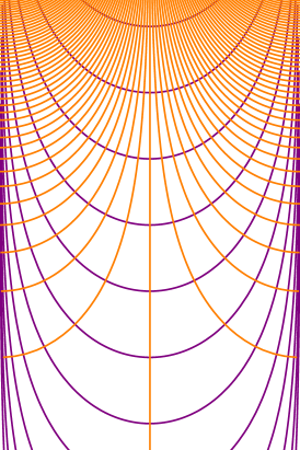
(a) The mapping $z\mapsto\mathbbm{i}\,e^{-\mathbbm{i}\pi z}$ is conformal from the the strip ${\mathbb{S}}$ to the half plane $\mathbb{H}$: the level lines of its real and imaginary parts are shown here.

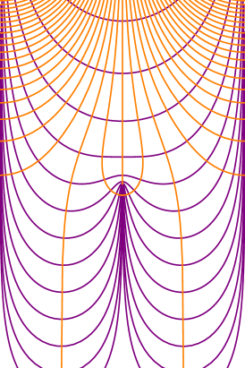
(b) The mapping $z\mapsto\varphi(z)$ is conformal from the the slit-strip ${\mathbb{S}}_{\mathrm{slit}}$ to the half plane $\mathbb{H}$: the level lines of its real and imaginary parts are shown here.

Figure 2.3. Illustrations of conformal maps to the strip and the slit-strip.

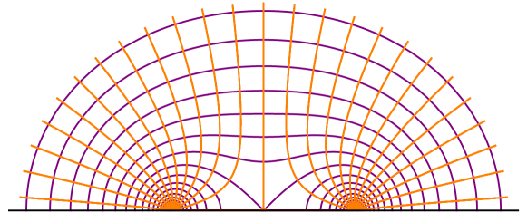
Figure 2.4. Illustration of the conformal map $\varphi\colon{\mathbb{S}}_{\mathrm{slit}}\to\mathbb{H}$ from the slit-strip to the half-plane: the images in the half-plane of horizontal and vertical lines in the slit-strip are shown here.

Illustrations of this conformal map (2.24) are given in Figures 2.3 and 2.4. Note the asymptotics in the three extremities of the slit-strip

$$\varphi(z)=\; \frac{\mathbbm{i}}{2}\,e^{-\pi\mathbbm{i}z}+\mathcal{O}(e^{\pi\mathbbm{i}z}), \varphi^{\prime}(z)=\; \frac{\pi}{2}\,e^{-\pi\mathbbm{i}z}+\mathcal{O}(e^{\pi\mathbbm{i}z})$$ in the top,

$$\varphi(z)=\; \frac{-1}{2}+\frac{1}{4}\,e^{-2\pi\mathbbm{i}z}+\mathcal{O}(e^{-4\pi\mathbbm{i}z}), \varphi^{\prime}(z)=\; \frac{-\pi\mathbbm{i}}{2}e^{-2\pi\mathbbm{i}z}+\mathcal{O}(e^{-4\pi\mathbbm{i}z})$$ in the left leg,

$$\varphi(z)=\; \frac{+1}{2}-\frac{1}{4}\,e^{-2\pi\mathbbm{i}z}+\mathcal{O}(e^{-4\pi\mathbbm{i}z}), \varphi^{\prime}(z)=\; \frac{+\pi\mathbbm{i}}{2}e^{-2\pi\mathbbm{i}z}+\mathcal{O}(e^{-4\pi\mathbbm{i}z})$$ in the right leg.

To use the conformal map $\varphi$ for unique pull-backs of $\frac{1}{2}$-forms, let us fix a branch of the square root of the derivative

$$\sqrt{\varphi^{\prime}}\,\colon{\mathbb{S}}_{\mathrm{slit}}\to\mathbb{C}\setminus\left\{0\right\}$$

so that $\sqrt{\varphi^{\prime}(x^{\mathrm{L}}_{0})}\in e^{\mathbbm{i}\pi/4}\,\mathbb{R}_{+}$ for boundary points $x^{\mathrm{L}}_{0}$ on the left boundaries and $\sqrt{\varphi^{\prime}(x^{\mathrm{R}}_{0})}\in e^{-\mathbbm{i}\pi/4}\,\mathbb{R}_{+}$ for boundary points $x^{\mathrm{R}}_{0}$ on the right boundaries. With this branch choice the asymptotics in the three extremities of the slit-strip are

$$\sqrt{\varphi^{\prime}(z)}=\; \sqrt{\frac{\pi}{2}}\,e^{-\mathbbm{i}\pi z/2}+\mathcal{O}(e^{\mathbbm{i}3\pi z/2})$$ in the top,

$$\sqrt{\varphi^{\prime}(z)}=\; \sqrt{\frac{\pi}{2}}\,e^{-\mathbbm{i}\pi(z+\frac{1}{4})}+\mathcal{O}(e^{-\mathbbm{i}3\pi z})$$ in the left leg,

$$\sqrt{\varphi^{\prime}(z)}=\; \sqrt{\frac{\pi}{2}}\,e^{-\mathbbm{i}\pi(z-\frac{1}{4})}+\mathcal{O}(e^{-\mathbbm{i}3\pi z})$$ in the right leg.

Define, for $k\in\pm\mathcal{K}$ (although we will primarily use the case of positive half-integer $k\in\mathcal{K}$), functions $\tilde{{P}}^{\mathrm{T}}_{k},\tilde{{P}}^{\mathrm{L}}_{k},\tilde{{P}}^{\mathrm{R}}_{k}\colon{\mathbb{S}}_{\mathrm{slit}}\to\mathbb{C}$ by the formulas

$$\tilde{{P}}^{\mathrm{T}}_{k}(z):=\; \mathbbm{i}\;\varphi(z)^{k-\frac{1}{2}}\;\sqrt{\varphi^{\prime}(z)}$$

(2.25) $$\tilde{{P}}^{\mathrm{L}}_{k}(z):=\; \mathbbm{i}\;\big{(}\varphi(z)+\frac{1}{2}\big{)}^{-k-\frac{1}{2}}\;\sqrt{\varphi^{\prime}(z)}$$

$$\tilde{{P}}^{\mathrm{R}}_{k}(z):=\; \mathbbm{i}\;\big{(}\varphi(z)-\frac{1}{2}\big{)}^{-k-\frac{1}{2}}\;\sqrt{\varphi^{\prime}(z)}.$$

The functions (2.25) are holomorphic and have Riemann boundary values (2.5) in the slit-strip ${\mathbb{S}}_{\mathrm{slit}}$. Their asymptotics in the corresponding extremities are given by

$$\tilde{{P}}^{\mathrm{T}}_{k}(z)=\; \mathbbm{i}\,\sqrt{\frac{\pi}{2}}\,\Big{(}\frac{\mathbbm{i}}{2}\Big{)}^{k-\frac{1}{2}}\,e^{-\mathbbm{i}\pi kz}+\mathcal{O}(e^{-\mathbbm{i}\pi(k-2)z})$$ in the top,

$$\tilde{{P}}^{\mathrm{L}}_{k}(z)=\; e^{\mathbbm{i}\pi/4}\,\sqrt{\frac{\pi}{2}}\;4^{k+\frac{1}{2}}\;e^{\mathbbm{i}2\pi kz}+\mathcal{O}(e^{\mathbbm{i}2\pi(k-1)z})$$ in the left leg,

$$\tilde{{P}}^{\mathrm{R}}_{k}(z)=\; -e^{-\mathbbm{i}\pi/4}\sqrt{\frac{\pi}{2}}\,(-4)^{k+\frac{1}{2}}\,e^{\mathbbm{i}2\pi kz}+\mathcal{O}(e^{\mathbbm{i}2\pi(k-1)z})$$ in the right leg.

In particular, for any positive half-integer $k\in\mathcal{K}$, the singular parts of $\tilde{{P}}^{\mathrm{T}}_{k},\tilde{{P}}^{\mathrm{L}}_{k},\tilde{{P}}^{\mathrm{R}}_{k}$ in the corresponding extremities contain finitely many singular Fourier modes. Moreover, it is easy to see that these functions are regular in the other two extremities.

Pure pole functions in the slit-strip

From the pulled-back monomials above, through a simple upper triangular transformation, we can construct functions characterized by a single Fourier mode as their singular parts. The functions are illustrated in Figure 2.5.

Proposition 2.6.

For all positive half-integers $k\in\mathcal{K}$, there exist functions

$${p}^{\mathrm{T}}_{k},\;{p}^{\mathrm{L}}_{k},\;{p}^{\mathrm{R}}_{k}\;\in\;\mathscr{L}^{2}$$

characterized by the following singular parts:

$$\Pi_{\mathrm{T};\mathrm{pole}}({p}^{\mathrm{T}}_{k})=\; e_{k}, \Pi_{\mathrm{L};\mathrm{pole}}({p}^{\mathrm{T}}_{k})=\; 0, \Pi_{\mathrm{R};\mathrm{pole}}({p}^{\mathrm{T}}_{k})=\; 0,$$

(2.26) $$\Pi_{\mathrm{T};\mathrm{pole}}({p}^{\mathrm{L}}_{k})=\; 0, \Pi_{\mathrm{L};\mathrm{pole}}({p}^{\mathrm{L}}_{k})=\; e^{\mathrm{L}}_{-k}, \Pi_{\mathrm{R};\mathrm{pole}}({p}^{\mathrm{L}}_{k})=\; 0,$$

$$\Pi_{\mathrm{T};\mathrm{pole}}({p}^{\mathrm{R}}_{k})=\; 0, \Pi_{\mathrm{L};\mathrm{pole}}({p}^{\mathrm{R}}_{k})=\; 0, \Pi_{\mathrm{R};\mathrm{pole}}({p}^{\mathrm{R}}_{k})=\; e^{\mathrm{R}}_{-k}.$$

The functions ${p}^{\mathrm{T}}_{k},{p}^{\mathrm{L}}_{k},{p}^{\mathrm{R}}_{k}$ are the restrictions to the cross-section $\mathcal{I}$ of globally defined holomorphic functions ${P}^{\mathrm{T}}_{k},{P}^{\mathrm{L}}_{k},{P}^{\mathrm{R}}_{k}\colon{\mathbb{S}}_{\mathrm{slit}}\to\mathbb{C}$ with Riemann boundary values on the slit-strip, which we call the pure pole functions. We can express these pure pole functions as finite linear combinations of the pulled-back monomials (2.25) and vice versa,

$${P}^{\mathrm{T}}_{k}=\; \sum_{0<k^{\prime}\leq k}A^{\mathrm{T}}_{k,k^{\prime}}\,\tilde{{P}}^{\mathrm{T}}_{k^{\prime}}, {P}^{\mathrm{L}}_{k}=\; \sum_{0<k^{\prime}\leq k}A^{\mathrm{L}}_{k,k^{\prime}}\,\tilde{{P}}^{\mathrm{L}}_{k^{\prime}}, {P}^{\mathrm{R}}_{k}=\; \sum_{0<k^{\prime}\leq k}A^{\mathrm{R}}_{k,k^{\prime}}\,\tilde{{P}}^{\mathrm{R}}_{k^{\prime}},$$

$$\tilde{{P}}^{\mathrm{T}}_{k}=\; \sum_{0<k^{\prime}\leq k}B^{\mathrm{T}}_{k,k^{\prime}}\,{P}^{\mathrm{T}}_{k^{\prime}}, \tilde{{P}}^{\mathrm{L}}_{k}=\; \sum_{0<k^{\prime}\leq k}B^{\mathrm{L}}_{k,k^{\prime}}\,{P}^{\mathrm{L}}_{k^{\prime}}, \tilde{{P}}^{\mathrm{R}}_{k}=\; \sum_{0<k^{\prime}\leq k}B^{\mathrm{R}}_{k,k^{\prime}}\,{P}^{\mathrm{R}}_{k^{\prime}},$$

with certain real coefficients $A^{\mathrm{T}}_{k,k^{\prime}},A^{\mathrm{L}}_{k,k^{\prime}},A^{\mathrm{R}}_{k,k^{\prime}},B^{\mathrm{T}}_{k,k^{\prime}},B^{\mathrm{L}}_{k,k^{\prime}},B^{\mathrm{R}}_{k,k^{\prime}}$.

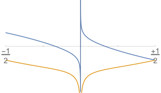
(a) The pole function ${p}^{\mathrm{T}}_{k}$ for $k=1/2$.

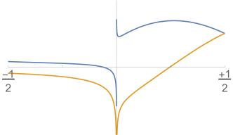
(b) The pole function ${p}^{\mathrm{R}}_{k}$ for $k=1/2$.

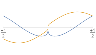
(c) The pole function ${p}^{\mathrm{T}}_{k}$ for $k=3/2$.

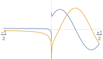
(d) The pole function ${p}^{\mathrm{R}}_{k}$ for $k=3/2$.

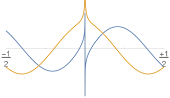
(e) The pole function ${p}^{\mathrm{T}}_{k}$ for $k=5/2$.

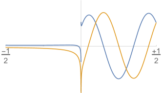
(f) The pole function ${p}^{\mathrm{R}}_{k}$ for $k=5/2$.

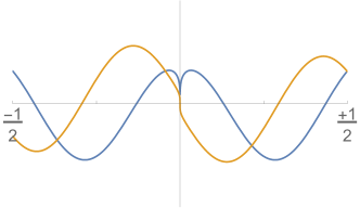
(g) The pole function ${p}^{\mathrm{T}}_{k}$ for $k=7/2$.

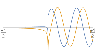
(h) The pole function ${p}^{\mathrm{R}}_{k}$ for $k=7/2$.

Figure 2.5. Real and imaginary parts (blue and orange) of the restrictions ${p}^{\mathrm{T}}_{k},{p}^{\mathrm{R}}_{k}$ to $\mathcal{I}$ of the pure pole functions ${P}^{\mathrm{T}}_{k},{P}^{\mathrm{R}}_{k}$ for the top and right extremities. (The pure pole functions ${P}^{\mathrm{L}}_{k}$ for the left leg, and their restrictions ${p}^{\mathrm{L}}_{k}$, are similar to the ones for the right leg.)

Proof.

We sketch the recursive construction of ${P}^{\mathrm{T}}_{k}$ in terms of pulled-back monomials; the other cases are analogous, and the resulting functions are uniquely characterized by (2.26) from Lemma 2.5.

First, note that we may define ${P}^{\mathrm{T}}_{1/2}=-\sqrt{\frac{2}{\pi}}\tilde{{P}}^{\mathrm{T}}_{1/2}$. If ${P}^{\mathrm{T}}_{k}$ for $k=1/2,\ldots,k^{\prime}$ are already constructed, we may define

$${P}^{\mathrm{T}}_{k^{\prime}+1}=\; \frac{(-1)^{k+\frac{1}{2}}2^{k}}{\sqrt{\pi}}\,\tilde{{P}}^{\mathrm{T}}_{k^{\prime}+1}-\sum_{0<k\leq k^{\prime}}\langle e_{k},\tilde{\mathfrak{q}}_{\mathrm{T};k^{\prime}+1}\rangle\,{P}^{\mathrm{T}}_{k},$$

where $\tilde{\mathfrak{q}}_{\mathrm{T};k}$ is the restriction of $\tilde{{P}}^{\mathrm{T}}_{k}$ to the real line.

Given the existence of pure pole functions, we may express the pulled-back monomials in terms of them as follows. By definition, there exist real coefficients $a_{-k^{\prime}}$ such that

$${P}^{\mathrm{T}}_{k}(z)=\; E_{k}(z)+\sum_{k^{\prime}>0}a_{-k^{\prime}}\,E_{-k^{\prime}}(z)\qquad\text{ for }z\in{\mathbb{S}}_{\mathrm{slit}}\cap\mathbb{H}.$$

Consider the conformal map $\tilde{w}=\mathbbm{i}\,e^{-\pi\mathbbm{i}z}$ from the slit-strip to the slit upper half-plane ${\mathbb{H}\setminus[0,\mathbbm{i}]}$. Under a change of variable analogous to (2.25),

$$E_{k}(z(\tilde{w}))\cdot\left[\frac{dz}{d\tilde{w}}\right]^{\frac{1}{2}} =\frac{e^{-\mathbbm{i}\pi k}}{\sqrt{\pi}}\tilde{w}^{k-\frac{1}{2}};$$

and thus

$${P}^{\mathrm{T}}_{k}(z(\tilde{w}))\cdot\left[\frac{dz}{d\tilde{w}}\right]^{\frac{1}{2}} =\frac{e^{-\mathbbm{i}\pi k}}{\sqrt{\pi}}\tilde{w}^{k-\frac{1}{2}}+\sum_{k^{\prime}>0}\frac{e^{\mathbbm{i}\pi k^{\prime}}a_{-k^{\prime}}}{\sqrt{\pi}}\tilde{w}^{-k^{\prime}-\frac{1}{2}}.$$

Since $\varphi(z)=\frac{1}{2}\sqrt{1+\tilde{w}(z)^{2}}$ and $\tilde{{P}}^{\mathrm{T}}_{k}$ is defined precisely as pullbacks of half-plane monomials,

$$\tilde{{P}}^{\mathrm{T}}_{k}(z(\tilde{w}))\cdot\left[\frac{dz}{d\tilde{w}}\right]^{\frac{1}{2}}=\; \mathbbm{i}\left(\frac{\sqrt{1+\tilde{w}^{2}}}{2}\right)^{k-\frac{1}{2}}\left[\frac{\tilde{w}}{2\sqrt{1+\tilde{w}^{2}}}\right]^{\frac{1}{2}}=\frac{\mathbbm{i}\sqrt{\tilde{w}}}{2^{k}}\left(1+\tilde{w}^{2}\right)^{\frac{k-1}{2}}$$

$$=\; \frac{\mathbbm{i}\tilde{w}^{k-\frac{1}{2}}}{2^{k}}\left(1+{\frac{k-1}{2}\choose{1}}\tilde{w}^{-2}+\cdots\right)\mbox{ as }\tilde{w}\to\infty.$$

The above binomial expansion only has finitely many terms with nonnegative powers of $w$, and their coefficients are precisely the coefficients in the expansion of $\tilde{{P}}^{\mathrm{T}}_{k}$ in terms of the pure pole functions:

$$\tilde{{P}}^{\mathrm{T}}_{k}=\; \sum_{0<k^{\prime}\leq k}\frac{\sqrt{\pi}e^{\mathbbm{i}\pi k^{\prime}}\mathbbm{i}}{2^{k}}{\frac{k-1}{2}\choose{\frac{k-k^{\prime}}{2}}}{P}^{\mathrm{T}}_{k^{\prime}},$$

where the binomial coefficient is taken as zero when $\frac{k-k^{\prime}}{2}$ is not an integer. The other cases are similar. ∎

Remark 2.7.

The coefficients in Proposition 2.6 implement a change of basis, which reflects the relationship of the geometry of the slit-strip ${\mathbb{S}}_{\mathrm{slit}}$ and the half-plane $\mathbb{H}$ via the conformal map (2.24) between them. These constants of geometric origin appear in our main result, which reconstructs the structure constants of the vertex operator algebra (the Ising conformal field theory) from the scaling limits of the fusion coefficients of the Ising model in lattice slit-strips.

Given that these constants thus account for the most nontrivial geometric input to our main result, we note that explicit expressions for them can be obtained similarly to the above proof by expanding monomials of the map (between the slit half-plane and the half-plane) $\psi(\tilde{w})=\frac{\sqrt{1+\tilde{w}^{2}}}{2}$ and its inverse. In the following, we will write $w$ for the variable in the half-plane, and $\tilde{w}$ for the slit half-plane; the boundary point $0$ in the slit half-plane corresponds to two prime ends $0_{-},0_{+}$, approached from left and right respectively.

Also note that we are considering holomorphic functions in a neighborhood of a boundary pole where they have Riemann boundary values. Using a pull-back to the half-plane, we may define their Schwarz reflection, which may be uniquely expanded in a Laurent series: this guarantees the existence and uniqueness of the expansions.

The constants can then be expressed as follows:

(2.27) $$A^{\mathrm{T}}_{k,k^{\prime}} =\mbox{ $(-\mathbbm{i})\cdot$(coefficient of $w^{k^{\prime}-\frac{1}{2}}$ of $\frac{e^{-\mathbbm{i}\pi k}}{\sqrt{\pi}}{\left(\sqrt{4w^{2}-1}\right)^{k-\frac{1}{2}}}\left[\frac{4w}{\sqrt{4w^{2}-1}}\right]^{\frac{1}{2}}$ around ${w}=\infty$)},$$

$$A^{\mathrm{L}}_{k,k^{\prime}} =\mbox{ $(-\mathbbm{i})\cdot$(coefficient of $(w+\frac{1}{2})^{-k^{\prime}-\frac{1}{2}}$ of $\sqrt{2}\mathbbm{i}\left({\sqrt{4w^{2}-1}}\right)^{-2k-\frac{1}{2}}\left[\frac{4w}{\sqrt{4w^{2}-1}}\right]^{\frac{1}{2}}$ around ${w}=-\frac{1}{2}$)},$$

$$A^{\mathrm{R}}_{k,k^{\prime}} =\mbox{ $(-\mathbbm{i})\cdot$(coefficient of $(w-\frac{1}{2})^{-k^{\prime}-\frac{1}{2}}$ of $\sqrt{2}e^{-\pi\mathbbm{i}k}\left({\sqrt{4w^{2}-1}}\right)^{-2k-\frac{1}{2}}\left[\frac{4w}{\sqrt{4w^{2}-1}}\right]^{\frac{1}{2}}$ around ${w}=\frac{1}{2}$)},$$

$$B^{\mathrm{T}}_{k,k^{\prime}} =\mbox{ $e^{\mathbbm{i}\pi k^{\prime}}\sqrt{\pi}\cdot$ (coefficient of $\tilde{w}^{k^{\prime}-\frac{1}{2}}$ of $\mathbbm{i}\left(\frac{\sqrt{1+\tilde{w}^{2}}}{2}\right)^{k-\frac{1}{2}}\left[\frac{\tilde{w}}{2\sqrt{1+\tilde{w}^{2}}}\right]^{\frac{1}{2}}$ around $\tilde{w}=\infty$)},$$

$$B^{\mathrm{L}}_{k,k^{\prime}} =\mbox{ $\frac{1}{\sqrt{2}\mathbbm{i}}\cdot$(coefficient of $\tilde{w}^{2k^{\prime}-\frac{1}{2}}$ of $\mathbbm{i}\left(\frac{\sqrt{1+\tilde{w}^{2}}}{2}+\frac{1}{2}\right)^{-k-\frac{1}{2}}\left[\frac{\tilde{w}}{2\sqrt{1+\tilde{w}^{2}}}\right]^{\frac{1}{2}}$ around $\tilde{w}=0_{-}$)},$$

$$B^{\mathrm{R}}_{k,k^{\prime}} =\mbox{ $\frac{e^{\pi\mathbbm{i}k^{\prime}}}{\sqrt{2}}\cdot$(coefficient of $\tilde{w}^{2k^{\prime}-\frac{1}{2}}$ of $\mathbbm{i}\left(\frac{\sqrt{1+\tilde{w}^{2}}}{2}-\frac{1}{2}\right)^{-k-\frac{1}{2}}\left[\frac{\tilde{w}}{2\sqrt{1+\tilde{w}^{2}}}\right]^{\frac{1}{2}}$ around $\tilde{w}=0_{+}$)}.$$

In particular, we have

$$A^{\mathrm{T}}_{k,k^{\prime}} =\left(\frac{-1}{4}\right)^{\frac{k-k^{\prime}}{2}}{{\frac{k-1}{2}}\choose{\frac{k-k^{\prime}}{2}}}, B^{\mathrm{T}}_{k,k^{\prime}} =\frac{\sqrt{\pi}e^{\mathbbm{i}\pi k^{\prime}}\mathbbm{i}}{2^{k}}{\frac{k-1}{2}\choose{\frac{k-k^{\prime}}{2}}}.$$

3. Discrete function spaces and decompositions

In this section we study functions on discretized domains, which have the properties analogous to holomorphicity and Riemann boundary values. We introduce the spaces of functions analogous to the continuum case, and find analogous distinguished functions: vertical translation eigenfunctions in the lattice strip, and functions with prescribed singularities in the extremities of the lattice slit-strip.

As the appropriate notion of discrete holomorphicity we use s-holomorphicity. This notion and its powerful uses together with Riemann boundary values were pioneered by Smirnov [Smi06, Smi10a], and have been developed into an extremely powerful tool for the study of the Ising model [ChSm11, ChSm12]. We have chosen a route to the main result of this series which avoids entirely the use of the notions of s-holomorphic poles [HoSm13, Hon10] and s-holomorphic spinors [Izy11, ChIz13, CHI15] and square root singularities. The quintessential trick for s-holomorphic solutions to Riemann boundary value problem is the “imaginary part of the integral of the square”, and we will be able to employ it largely in its most standard incarnation in Section 4.

In Section 3.1 we introduce the discrete domains, and in Section 3.2 give the definitions of the needed notions of discrete complex analysis and of the space of functions of interest to us. In Section 3.4 we study the vertical translation eigenfunctions in the strip, and the associated decomposition of the function space. In Section 3.4 we find the distinguished functions in the lattice slit-strip, which have prescribed singularities in the extremities.

3.1. The lattice strip and the lattice slit-strip

The lattice analogues of the continuum strip and slit-strip domains ${\mathbb{S}}$ and ${\mathbb{S}}_{\mathrm{slit}}$ will be certain square grid discretizations of these domains.

Fix two integers

$$a,b\in\mathbb{Z},\qquad a<0<b,$$

which represent the (horizontal) positions of the left and right boundaries. The slit will always be placed at the horizontal position $0$. The width of the strip (in lattice units) is

(3.1) $$0pt:=b-a\;\in\,\mathbb{N}.$$

For simplicity of notation, we only carry the superscript label for width $0pt$ in the notation to indicate the discretization, although information about $a$ and $b$ is in fact important as well. We mostly care about a symmetric situation (equal widths for the left and right substrip) in which $b=-a=\frac{1}{2}0pt$ and the limit of large even integer widths $0pt\to\infty$, but more general choices are possible and at times in fact clearer.

The lattice strip

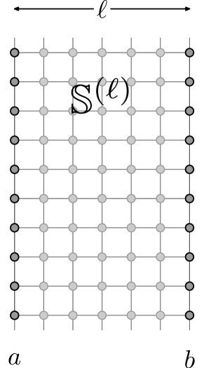
(a) The square grid strip ${{\mathbb{S}}^{(0pt)}}$.

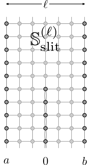
(b) The square grid slit-strip ${{\mathbb{S}}_{\mathrm{slit}}^{(0pt)}}$.

Figure 3.1. The discrete strip and slit-strip graphs.

A discretized version of the cross-section $\mathcal{I}$ is the integer interval

(3.2) $$I:=\; \left\{a,a+1,a+2,\ldots,b-1,b\right\}=:\llbracket a,b\rrbracket.$$

The lattice strip is then defined as the graph with vertex set

(3.3) $${{\mathbb{S}}^{(0pt)}}:=\; \left\{x+\mathbbm{i}y\;\Big{|}\;x\in I,\;y\in\mathbb{Z}\right\}=\llbracket a,b\rrbracket\times\mathbb{Z},$$

and with nearest neighbor edges as in Figure 3.1(a) — in other words, the lattice strip is seen as an induced subgraph ${{\mathbb{S}}^{(0pt)}}\subset\mathbb{Z}^{2}$ of the ordinary square lattice.

The set of all edges of the lattice strip is denoted by $\mathrm{E}({{\mathbb{S}}^{(0pt)}})$. We will identify edges with their midpoints, so that vertical edges are of the form $x+\mathbbm{i}y^{\prime}\in\mathrm{E}({{\mathbb{S}}^{(0pt)}})$ with $x\in I$ and $y^{\prime}\in\mathbb{Z}+\frac{1}{2}$, and horizontal edges are of the form $x^{\prime}+\mathbbm{i}y\in\mathrm{E}({{\mathbb{S}}^{(0pt)}})$ with $y\in\mathbb{Z}$ and $x^{\prime}\in I^{*}$ in the half-integer interval defined by

(3.4) $$I^{*}:=\; \left\{a+\frac{1}{2},a+\frac{3}{2},\ldots,b-\frac{3}{2},b-\frac{1}{2}\right\}=:\llbracket a,b\rrbracket^{*}.$$

In fact, it is this half-integer interval $I^{*}$ on which our functions will be defined.

Lattice slit-strip

The lattice slit-strip will be the (multi-)graph with the same set of vertices

(3.5) $${{\mathbb{S}}_{\mathrm{slit}}^{(0pt)}}:=\; \left\{x+\mathbbm{i}y\;\Big{|}\;x\in I,\;y\in\mathbb{Z}\right\}=\llbracket a,b\rrbracket\times\mathbb{Z}$$

as the lattice strip, and otherwise also the same set of edges, except that there are double edges between nearest neighbors $0+\mathbbm{i}y$ and $0+\mathbbm{i}(y-1)$ for $y\leq 0$, i.e., along the slit. This is illustrated in Figure 3.1(b). The two different edges between nearest neighbors on the slit part have exactly the same roles as the two different prime-ends corresponding to the same boundary point on the slit in the continuum slit-strip ${\mathbb{S}}_{\mathrm{slit}}$ of Figure 2.1(b): one is thought to belong to (the boundary of) the left substrip and the other to (the boundary of) the right substrip.

The set of all edges of the lattice slit-strip is denoted by $\mathrm{E}({{\mathbb{S}}_{\mathrm{slit}}^{(0pt)}})$. Despite the presence of multi-edges, we continue to abuse the notation and usually label edges of the lattice slit-strip by their midpoints. For any pair of edges along the slit which have coinciding midpoints, we trust that it will always be sufficiently clear from the context which one of the two edges is meant (it should be clear whether we are considering the left or the right substrip).

3.2. S-holomorphicity, Riemann boundary values, and function spaces

In this discrete setting, functions will be defined on the edges of the graph. We allow for functions defined on subgraphs as well, so let $\mathrm{V}$ denote the relevant (sub)set of vertices ($\mathrm{V}\subset{{\mathbb{S}}^{(0pt)}}={{\mathbb{S}}_{\mathrm{slit}}^{(0pt)}}$) and $\mathrm{E}$ the relevant (sub)set of edges ($\mathrm{E}\subset\mathrm{E}({{\mathbb{S}}^{(0pt)}})$ or $\mathrm{E}\subset\mathrm{E}({{\mathbb{S}}_{\mathrm{slit}}^{(0pt)}})$). We consider functions

$$F\colon\mathrm{E}\to\mathbb{C}.$$

S-holomorphicity

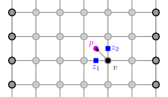
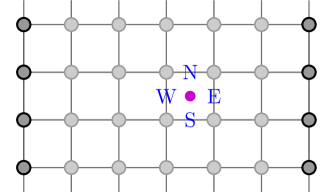
Figure 3.2. S-holomorphicity is a condition for the values of a function on pairs of edges $z_{1},z_{2}$ adjacent to the same face $p$ and vertex $v$.

A function $F\colon\mathrm{E}\to\mathbb{C}$ is said to be s-holomorphic, if for all pairs of edges $z_{1},z_{2}\in\mathrm{E}$ which are adjacent, in the sense that both are adjacent to the same face $p$ and the same vertex $v$, we have

(3.6) $$F(z_{1})+\frac{\mathbbm{i}\,|v-p|}{v-p}\,\overline{F(z_{1})}=F(z_{2})+\frac{\mathbbm{i}\,|v-p|}{v-p}\,\overline{F(z_{2})}.$$

Equivalently, the values of $F$ at $z_{1}$ and $z_{2}$ have the same projections to the line $\sqrt{\mathbbm{i}/(v-p)}\,\mathbb{R}$ in the complex plane. Depending on the position of the adjacent edges $z_{1},z_{2}$ with respect to the face, this line is one among four possibilities. In view of this, yet another explicit way of writing the s-holomorphicity condition is the following. Define the constant

$$\lambda=e^{\mathbbm{i}\pi/4}=\frac{1+\mathbbm{i}}{\sqrt{2}}$$

that we will keep using throughout, as is common in related literature. The s-holomorphicity condition is equivalent to requiring that when $\mathrm{N},\mathrm{E},\mathrm{S},\mathrm{W}$ are the four edges surrounding a face as in Figure 3.2, then

$$F(\mathrm{N})+\lambda^{-1}\overline{F(\mathrm{N})} =F(\mathrm{W})+\lambda^{-1}\overline{F(\mathrm{W})},\quad F(\mathrm{N})+\lambda\overline{F(\mathrm{N})} =F(\mathrm{E})+\lambda\overline{F(\mathrm{E})},$$

$$F(\mathrm{S})+\lambda^{-3}\overline{F(\mathrm{S})} =F(\mathrm{W})+\lambda^{-3}\overline{F(\mathrm{W})},\quad F(\mathrm{S})+\lambda^{3}\overline{F(\mathrm{S})} =F(\mathrm{E})+\lambda^{3}\overline{F(\mathrm{E})}.$$

S-holomorphicity implies (but is not implied by) the usual discretized Cauchy-Riemann equations

$$F(z+\frac{1}{2})-F(z-\frac{1}{2})=-\mathbbm{i}\,\Big{(}F(z+\frac{\mathbbm{i}}{2})-F(z-\frac{\mathbbm{i}}{2})\Big{)}$$

around any face or vertex $z$ where all the needed values are defined. This at least gives the interpretation for s-holomorphicity as a notion of discrete holomorphicity, which may not have been apparent directly from definition (3.6). Note, however, that s-holomorphicity is an $\mathbb{R}$-linear condition for the complex-valued function $F$ — not $\mathbb{C}$-linear!

Riemann boundary values

The discrete version of Riemann boundary values is defined very analogously to the continuum version. If $z\in\mathrm{E}$ is a boundary edge, and $\tau(z)$ denotes the unit complex number in the direction of the tangent to the boundary oriented counterwlockwise (i.e., so that the face to the left of the oriented edge is a part of the discrete domain), then $F$ is said to have a Riemann boundary value at $z$ if

(3.7) $$F(z)\in\mathbbm{i}\,\tau(z)^{-1/2}\,\mathbb{R}.$$

We will only use Riemann boundary values on the boundaries of the lattice strip and lattice slit-strip. These boundaries are taken to consist of the vertical edges on the left and on the right as well as on the slit. The vertical edges on the left boundary are of the form $z=a+\mathbbm{i}y^{\prime}$ with $y^{\prime}\in\mathbb{Z}+\frac{1}{2}$ and their counterclockwise tangent points downwards, $\tau(z)=-\mathbbm{i}$. The vertical edges on the right boundary are of the form $z=b+\mathbbm{i}y^{\prime}$ with $y^{\prime}\in\mathbb{Z}+\frac{1}{2}$ and their counterclockwise tangent points upwards, $\tau(z)=+\mathbbm{i}$. The requirement of Riemann boundary values for functions in the lattice strip ${{\mathbb{S}}^{(0pt)}}$ are thus

(3.8) $$F\big{(}a+\mathbbm{i}y^{\prime}\big{)}\in e^{-\mathbbm{i}\pi/4}\,\mathbb{R}\qquad\text{ and }\qquad F\big{(}b+\mathbbm{i}y^{\prime}\big{)}\in e^{+\mathbbm{i}\pi/4}\,\mathbb{R}$$

for $y^{\prime}\in\mathbb{Z}+\frac{1}{2}$.

The slit part of the boundary has doubled edges, one for the left side of the slit (which acts as a right boundary for the left substrip) and one for the right side (which acts as a left boundary to the right substrip). Denoting these edges respectively by $z=0^{-}+\mathbbm{i}y^{\prime}$ and $z=0^{+}+\mathbbm{i}y^{\prime}$, the Riemann boundary values on the slit part are

(3.9) $$F\big{(}0^{-}+\mathbbm{i}y^{\prime}\big{)}\in e^{+\mathbbm{i}\pi/4}\,\mathbb{R}\qquad\text{ and }\qquad F\big{(}0^{+}+\mathbbm{i}y^{\prime}\big{)}\in e^{-\mathbbm{i}\pi/4}\,\mathbb{R}$$

for $y^{\prime}\in\mathbb{Z}+\frac{1}{2}$, $y^{\prime}<0$.

Note the analogy of (3.8) and (3.9) with (2.4) and (2.5), and note once more that Riemann boundary values are $\mathbb{R}$-linear conditions for the complex-valued function $F$.

Functions on the discrete cross-section

Analogously to the continuum approach in Section 2.1, we study s-holomorphic functions with Riemann boundary values on the lattice strip ${{\mathbb{S}}^{(0pt)}}$ and lattice slit-strip ${{\mathbb{S}}_{\mathrm{slit}}^{(0pt)}}$ through their restrictions to the horizontal cross-sections at height zero. These cross-sections consist of the $0pt$ horizontal edges whose midpoints are $x^{\prime}\in I^{*}$ as in (3.4).

The space

(3.10) $$\mathscr{F}^{(0pt)}:=\; \mathbb{C}^{I^{*}}$$

is thought of as the space of all complex valued functions $f\colon I^{*}\to\mathbb{C}$ on the discrete cross-section $I^{*}$. Because the main operations we consider are $\mathbb{R}$-linear, we interpret $\mathscr{F}^{(0pt)}$ as a real vector space of dimension

$$\mathrm{dim}_{\mathbb{R}}(\mathscr{F}^{(0pt)})=20pt.$$

We equip it with the inner product defined by the formula

(3.11) $$\langle f,g\rangle=\sum_{x^{\prime}\in I^{*}}\Big{(}\Re\mathfrak{e}\big{(}f(x^{\prime})\big{)}\,\Re\mathfrak{e}\big{(}g(x^{\prime})\big{)}+\Im\mathfrak{m}\big{(}f(x^{\prime})\big{)}\,\Im\mathfrak{m}\big{(}g(x^{\prime})\big{)}\Big{)}$$

for $f,g\in\mathscr{F}^{(0pt)}$. This inner product induces the familiar norm

$$\|f\|=\Big{(}\sum_{x^{\prime}\in I^{*}}|f(x^{\prime})|^{2}\Big{)}^{1/2}.$$

3.3. Vertical translation eigenfunctions in the lattice strip

In Section 2.2 we saw that among the holomorphic functions with Riemann boundary values in the strip, the vertical translation eigenfunctions were exactly the extensions of quarter integer Fourier modes on the cross-section. Here we address the analogous discrete question.

Discrete analytic continuation by one vertical step

The operation of discrete analytic continuation by one vertical step was considered in [HKZ14]. We take from there the following result, whose proof is a straightforward calculation from definitions (3.6) and (3.8).

Proposition 3.1 ([HKZ14, Lemmas 4 and 6]).

For any $f\in\mathscr{F}^{(0pt)}$, there exists a unique function $F\colon\mathrm{E}({{\mathbb{S}}^{(0pt)}})\to\mathbb{C}$ which is s-holomorphic and has Riemann boundary values in the lattice strip ${{\mathbb{S}}^{(0pt)}}$, and whose restriction to the discrete cross-section coincides with $f$:

$$F(x^{\prime})=f(x^{\prime})\qquad\text{for all }x^{\prime}\in I^{*}\subset\mathrm{E}({{\mathbb{S}}^{(0pt)}}).$$

If we define a new function $\mathsf{A}f\colon I^{*}\to\mathbb{C}$ in terms of this extension $F$ by

$$\big{(}\mathsf{A}f\big{)}(x^{\prime}):=F(x^{\prime}+\mathbbm{i})\qquad\text{for }x^{\prime}\in I^{*},$$

then $\mathsf{A}f$ is explicitly given by

$$\big{(}\mathsf{A}f\big{)}(x^{\prime})=\; 2\,f(x^{\prime})+\frac{\lambda^{3}}{\sqrt{2}}\,f(x^{\prime}+1)+\frac{\lambda^{-3}}{\sqrt{2}}\,f(x^{\prime}-1)$$

$$-\sqrt{2}\;\overline{f(x^{\prime})}+\frac{1}{\sqrt{2}}\,\overline{f(x^{\prime}+1)}+\frac{1}{\sqrt{2}}\,\overline{f(x^{\prime}-1)}\qquad x^{\prime}\neq a+\frac{1}{2},b-\frac{1}{2}$$ for ,

$$\big{(}\mathsf{A}f\big{)}(x^{\prime}_{\mathrm{L}})=\; \Big{(}1+\frac{1}{\sqrt{2}}\Big{)}\,f(x^{\prime}_{\mathrm{L}})+\frac{\lambda^{3}}{\sqrt{2}}\,f(x^{\prime}_{\mathrm{L}}+1)$$

$$+\Big{(}\lambda^{3}+\frac{\lambda^{-3}}{\sqrt{2}}\Big{)}\,\overline{f(x^{\prime}_{\mathrm{L}})}+\frac{1}{\sqrt{2}}\,\overline{f(x^{\prime}_{\mathrm{L}}+1)}\qquad x^{\prime}_{\mathrm{L}}=a+\frac{1}{2}$$ for ,

$$\big{(}\mathsf{A}f\big{)}(x^{\prime}_{\mathrm{R}})=\; \Big{(}1+\frac{1}{\sqrt{2}}\Big{)}\,f(x^{\prime}_{\mathrm{R}})+\frac{\lambda^{-3}}{\sqrt{2}}\,f(x^{\prime}_{\mathrm{R}}-1)$$

$$+\Big{(}\lambda^{-3}+\frac{\lambda^{3}}{\sqrt{2}}\Big{)}\,\overline{f(x^{\prime}_{\mathrm{R}})}+\frac{1}{\sqrt{2}}\,\overline{f(x^{\prime}_{\mathrm{R}}-1)}\qquad x^{\prime}_{\mathrm{R}}=b-\frac{1}{2}$$ for ,

where $\lambda=e^{\mathbbm{i}\pi/4}$. The mapping $f\mapsto\mathsf{A}f$ defines a linear operator

$$\mathsf{A}\colon\mathscr{F}^{(0pt)}\to\mathscr{F}^{(0pt)}.$$

By the above it is clear that $F\colon\mathrm{E}({{\mathbb{S}}^{(0pt)}})\to\mathbb{C}$ is a vertical translation eigenfunction if and only if its restriction $f=F\big{|}_{I^{*}}$ to the discrete cross-section is an eigenfunction of the operator $\mathsf{A}$. More precisely for any $\Lambda\neq 0$, the property

$$F(z+\mathbbm{i}h)=\Lambda^{h}\;F(z)\qquad\text{ for all }z\in\mathrm{E}({{\mathbb{S}}^{(0pt)}})\text{ and }h\in\mathbb{Z}$$

is equivalent to

$$\mathsf{A}f=\Lambda\,f.$$

In [HKZ14] many qualitative properties of the spectrum of $\mathsf{A}$ were proven directly: it is symmetric, invertible, conjugate to its own inverse, all eigenvalues have multiplicity one, and $1$ is not an eigenvalue. Moreover, the complexification of $\mathsf{A}$ was shown to be conjugate to the induced rotation of the Ising transfer matrix with locally monochromatic boundary conditions, whose spectrum is well-known [AbMa73, Pal07]. We will need the eigenvectors and eigenvalues explicitly, and we thus rederive such properties via a direct calculation below.

The following qualitative property related to reflections across the cross-section is, however, instructive and useful to note first.

Remark 3.2.

For any vertical translation eigenfunction that is exponentially growing in the upwards direction, there is a corresponding vertical translation eigenfunction that is exponentially growing in the downwards direction. Namely if $F\colon\mathrm{E}({{\mathbb{S}}^{(0pt)}})\to\mathbb{C}$ is s-holomorphic and has Riemann boundary values, then also $\widetilde{F}\colon\mathrm{E}({{\mathbb{S}}^{(0pt)}})\to\mathbb{C}$ defined by

$$\widetilde{F}(x+\mathbbm{i}y)=-\mathbbm{i}\,\overline{F(x-\mathbbm{i}y)}$$

is s-holomorphic and has Riemann boundary values. If $F$ satisfies $F(z+\mathbbm{i}h)=\Lambda^{h}\,F(z)$ with $\Lambda\in\mathbb{R}\setminus\left\{0\right\}$, then $\widetilde{F}$ satisfies $\widetilde{F}(z+\mathbbm{i}h)=(1/\Lambda)^{h}\,\widetilde{F}(z)$.

In the function space $\mathscr{F}^{(0pt)}$, the corresponding operation

$$f\mapsto\tilde{f}=\mathsf{R}f,\qquad(\mathsf{R}f)(x^{\prime}):=-\mathbbm{i}\,\overline{f(x^{\prime})}$$

is a unitary involution $\mathsf{R}\colon\mathscr{F}^{(0pt)}\to\mathscr{F}^{(0pt)}$ by which $\mathsf{A}$ is conjugate to its inverse $\mathsf{A}^{-1}$.

A dispersion relation

The vertical translation eigenfunctions in the continuum strip are essentially the quarter-integer Fourier modes. The vertical translation eigenfunctions in the lattice strip turn out to be mixtures of two discrete Fourier modes with opposite frequencies. Which frequencies can appear is ultimately determined by the boundary conditions. Before addressing that, let us observe that a relation between the vertical translation eigenvalue and the frequency of the Fourier mode is obtained from the first of the formulas of Proposition 3.1, which governs the discrete analytic continuation away from boundaries.

Lemma 3.3.

Let $\omega\in\mathbb{R}\setminus 2\pi\mathbb{Z}$, and let $\Lambda$ be a solution to the equation

(3.12) $$\Lambda^{2}+\big{(}2\cos(\omega)-4\big{)}\,\Lambda+1=0.$$

Define

$$f(x^{\prime})=C^{+}\,e^{+\mathbbm{i}\omega x^{\prime}}+C^{-}\,e^{-\mathbbm{i}\omega x^{\prime}},\qquad\text{for }x^{\prime}\in I^{*},$$

where the constants $C^{+},C^{-}\in\mathbb{C}$ are related by

$$C^{-}=\frac{2+\sqrt{2}\,\cos(\frac{3\pi}{4}+\omega)-\Lambda}{\sqrt{2}\big{(}1-\cos(\omega)\big{)}}\;\overline{C^{+}}.$$

Then for any $x^{\prime}\in I^{*}\setminus\{a+\frac{1}{2},b-\frac{1}{2}\}$, we have $\big{(}\mathsf{A}f\big{)}(x^{\prime})=\Lambda\,f(x^{\prime})$.

Proof.

Inserting the defining formula of $f(x^{\prime})$ into the the explicit expression for $\big{(}\mathsf{A}f\big{)}(x^{\prime})$ from Proposition 3.1, a straightforward calculation yields

$$\big{(}\mathsf{A}f\big{)}(x^{\prime})-\Lambda\,f(x^{\prime})=\; \phantom{+}e^{+\mathbbm{i}\omega x^{\prime}}\left(C^{+}\Big{(}2+\sqrt{2}\cos\big{(}\frac{3\pi}{4}+\omega\big{)}-\Lambda\Big{)}+\overline{C^{-}}\Big{(}\sqrt{2}\cos(\omega)-\sqrt{2}\Big{)}\right)$$

$$+e^{-\mathbbm{i}\omega x^{\prime}}\left(C^{-}\Big{(}2+\sqrt{2}\cos\big{(}\frac{3\pi}{4}-\omega\big{)}-\Lambda\Big{)}+\overline{C^{+}}\Big{(}\sqrt{2}\cos(\omega)-\sqrt{2}\Big{)}\right).$$

Using the relationship between the constants $C^{+},C^{-}$, the coefficient of $e^{+\mathbbm{i}\omega x^{\prime}}$ above vanishes immediately. It remains to check the vanishing of the coefficient of $e^{-\mathbbm{i}\omega x^{\prime}}$.

For this purpose, observe that using the trigonometric identities $\cos\big{(}\frac{3\pi}{4}+\omega\big{)}+\cos\big{(}\frac{3\pi}{4}-\omega\big{)}=-\sqrt{2}\,\cos(\omega)$ and $\cos\big{(}\frac{3\pi}{4}+\omega\big{)}\cos\big{(}\frac{3\pi}{4}-\omega\big{)}=\frac{1}{2}\cos(2\omega)$ we can write

$$\Big{(}2+\sqrt{2}\,\cos(\frac{3\pi}{4}+\omega)-\Lambda\Big{)}\Big{(}2+\sqrt{2}\,\cos(\frac{3\pi}{4}-\omega)-\Lambda\Big{)}$$

$$=\; \Lambda^{2}-\big{(}4-2\cos(\omega)\big{)}\Lambda+4+\cos(2\omega)-4\cos(\omega).$$

When $\Lambda$ is a solution to (3.12), this expression further simplifies to

$$3+\cos(2\omega)-4\cos(\omega)=2\big{(}1-\cos(\omega)\big{)}^{2}.$$

We thus see that an alternative equivalent form of the relationship between the constants $C^{+},C^{-}$ is

$$C^{-}=\frac{\sqrt{2}\big{(}1-\cos(\omega)\big{)}}{2+\sqrt{2}\,\cos(\frac{3\pi}{4}-\omega)-\Lambda}\;\overline{C^{+}}.$$

From this relationship we immediately see the desired vanishing of the coefficient of $e^{-\mathbbm{i}\omega x^{\prime}}$, so the proof is complete. ∎

Remark 3.4.

For a given $\omega$, Equation (3.12) has two roots, which are positive real numbers and inverses of each other. This reflects the observation from Remark 3.2 by which vertical translation eigenfunctions can be reflected to produce eigenfunctions with the inverse eigenvalue. Indeed for functions of the form $f(x^{\prime})=C^{+}\,e^{+\mathbbm{i}\omega x^{\prime}}+C^{-}\,e^{-\mathbbm{i}\omega x^{\prime}}$ as above, $(\mathsf{R}f)(x^{\prime})=-\mathbbm{i}\overline{f(x^{\prime})}$ is also of the same form (with different coefficients), and it has the inverse eigenvalue for $\mathsf{A}$.

Boundary conditions and equation on frequencies

By the above calculation, the discrete Fourier modes of any frequency $\omega\in\mathbb{R}$ and its opposite can be combined to satisfy the equation $(\mathsf{A}f)(x^{\prime})=\Lambda\,f(x^{\prime})$ for $x^{\prime}$ not adjacent to the boundaries, provided that $\omega$ and $\Lambda$ are related by (3.12). However, such functions can satisfy the equation $(\mathsf{A}f)(x^{\prime})=\Lambda\,f(x^{\prime})$ near the boundaries only if the frequency is chosen judiciously. It is sufficient for us to prove that under a certain hypothesis on the frequency $\omega$, an eigenfunction exists; simple counting afterwards will show that all eigenfunctions are thus found.

Lemma 3.5.

Suppose that $\omega\in\mathbb{R}$ is a solution to

(3.13) $$\frac{\cos\big{(}(0pt+\frac{1}{2})\,\omega\big{)}}{\cos\big{(}(0pt-\frac{1}{2})\,\omega\big{)}}=3-2\sqrt{2},$$

and let $\Lambda$ be a solution to (3.12). Then there exists non-zero $f\in\mathscr{F}^{(0pt)}$ such that $\mathsf{A}f=\Lambda\,f$.

Proof.

Let us denote by

$$R=R(\omega,\Lambda)=\frac{2+\sqrt{2}\,\cos(\frac{3\pi}{4}+\omega)-\Lambda}{\sqrt{2}\big{(}1-\cos(\omega)\big{)}}.$$

the ratio in Lemma 3.3 which relates the coefficient of one Fourier mode to the complex conjugate of the coefficient of the opposite one. We will show that $f\in\mathscr{F}^{(0pt)}$ of the form

$$f(x^{\prime})=C\,e^{+\mathbbm{i}\omega x^{\prime}}+R\overline{C}\,e^{-\mathbbm{i}\omega x^{\prime}}$$

works, with suitably chosen $C\neq 0$.

Given the result of Lemma 3.3, the only remaining properties to verify are $(\mathsf{A}f)(x^{\prime}_{\mathrm{L}})=\Lambda\,f(x^{\prime}_{\mathrm{L}})$ and $(\mathsf{A}f)(x^{\prime}_{\mathrm{R}})=\Lambda\,f(x^{\prime}_{\mathrm{R}})$, where $x^{\prime}_{\mathrm{L}}=a+\frac{1}{2}$ and $x^{\prime}_{\mathrm{R}}=b-\frac{1}{2}$. In view of Proposition 3.1, these amount to the equations

$$0=\; C\,e^{\mathbbm{i}\omega x^{\prime}_{\mathrm{L}}}\Big{(}A^{+}+RB^{+}\Big{)}+\overline{C}\,e^{-\mathbbm{i}\omega x^{\prime}_{\mathrm{L}}}\Big{(}B^{-}+RA^{-}\Big{)}$$

$$0=\; C\,e^{\mathbbm{i}\omega x^{\prime}_{\mathrm{R}}}\Big{(}\overline{A^{+}}+R\overline{B^{+}}\Big{)}+\overline{C}\,e^{-\mathbbm{i}\omega x^{\prime}_{\mathrm{R}}}\Big{(}\overline{B^{-}}+R\overline{A^{-}}\Big{)},$$

where

$$A^{\pm}=A^{\pm}(\omega,\Lambda):=\; 1+\frac{1}{\sqrt{2}}+\frac{\lambda^{3}}{\sqrt{2}}e^{\pm\mathbbm{i}\omega}-\Lambda,$$

$$B^{\pm}=B^{\pm}(\omega):=\; \lambda^{3}+\frac{\lambda^{-3}}{\sqrt{2}}+\frac{1}{\sqrt{2}}e^{\pm\mathbbm{i}\omega}.$$

Either one of the two equations fixes the argument of $C$ modulo $\pi$, in that one can solve for $C/\overline{C}$ from them. The former equation requires

$$C/\overline{C}\,=\; -e^{-\mathbbm{i}2\omega x^{\prime}_{\mathrm{L}}}\;\frac{B^{-}+RA^{-}}{A^{+}+RB^{+}},$$

and after first taking complex conjugates, the second requires

$$C/\overline{C}\,=\; -e^{-\mathbbm{i}2\omega x^{\prime}_{\mathrm{R}}}\;\frac{A^{+}+RB^{+}}{B^{-}+RA^{-}}.$$

Evidently the modulus of these expressions are the inverses of each other, so when we have the equality of the two, the existence of nonzero $C\in\mathbb{C}$ satisfying the eigenfunction requirements follows. The equality of the two expressions simply reads

$$\frac{\big{(}A^{+}+RB^{+}\big{)}^{2}}{\big{(}B^{-}+RA^{-}\big{)}^{2}}=e^{\mathbbm{i}2(0pt-1)\omega}.$$

Our goal is therefore to show that this equality follows from our assumption (3.13) (in fact the two are equivalent). The numerator and denominator on the left hand side are by construction expressed as polynomials in $\Lambda$ of degrees $2$ and $4$, but since by assumption $\Lambda$ satisfies the quadratic equation (3.12), we can reduce both to first order polynomials in $\Lambda$. This is straightforward but slightly tedious. We first simplify the numerator and denominator before taking the squares

$$A^{+}(\omega,\Lambda)+R(\omega,\Lambda)\,B^{+}(\omega)=\; \frac{(1-\sqrt{2})\lambda\,\Lambda+e^{-\mathbbm{i}\omega}\,\Lambda+\lambda^{3}\,e^{-\mathbbm{i}\omega}+\mathbbm{i}(1-\sqrt{2})}{2(1-\cos(\omega))},$$

$$B^{-}(\omega)+R(\omega,\Lambda)\,A^{-}(\omega,\Lambda)=\; \frac{(\sqrt{2}-1)\,\Lambda-\lambda e^{\mathbbm{i}\omega}\,\Lambda+\mathbbm{i}\,e^{\mathbbm{i}\omega}+(\sqrt{2}-1)\lambda^{3}}{2(1-\cos(\omega))}.$$

and then take the squares and simplify further to

$$\big{(}A^{+}+RB^{+}\big{)}^{2}=\; \frac{(e^{\mathbbm{i}\omega}-1)\,e^{-\mathbbm{i}3\omega}}{4(1-\cos(\omega))^{2}}\,\Big{(}\big{(}1+\mathbbm{i}\,e^{\mathbbm{i}2\omega}-2\sqrt{2}\lambda e^{\mathbbm{i}\omega}\big{)}\Lambda+\sqrt{2}\lambda\,e^{\mathbbm{i}\omega}\Big{)}\,\big{(}1-(3-2\sqrt{2})e^{\mathbbm{i}\omega}\big{)}$$

$$\big{(}B^{-}+R\,A^{-}\big{)}^{2}=\; \frac{(e^{\mathbbm{i}\omega}-1)\,e^{-\mathbbm{i}\omega}}{4(1-\cos(\omega))^{2}}\,\Big{(}\big{(}1+\mathbbm{i}\,e^{\mathbbm{i}2\omega}-2\sqrt{2}\lambda e^{\mathbbm{i}\omega}\big{)}\Lambda+\sqrt{2}\lambda\,e^{\mathbbm{i}\omega}\Big{)}\,\big{(}(3-2\sqrt{2})-e^{\mathbbm{i}\omega}\big{)}.$$

Cancellations in the ratio of these two yield

$$\frac{\big{(}A^{+}+RB^{+}\big{)}^{2}}{\big{(}B^{-}+RA^{-}\big{)}^{2}}=\frac{\left(3-2\sqrt{2}\right)e^{\mathbbm{i}\omega}-1}{e^{\mathbbm{i}\omega}-(3-2\sqrt{2})}\;e^{-2\mathbbm{i}\omega}.$$

The desired equality of the expressions thus ultimately amounts to

$$\frac{\left(3-2\sqrt{2}\right)e^{\mathbbm{i}\omega}-1}{e^{\mathbbm{i}\omega}-(3-2\sqrt{2})}=e^{\mathbbm{i}20pt\omega},$$

which is easily seen to be equivalent to (3.13). This finishes the proof. ∎

Allowed frequencies

In the continuum, vertical translation eigenfunctions were associated to all quarter-integer Fourier modes. By contrast, in the discrete setup there are only finitely many possible frequencies, and these are only approximately quarter integers (in the appropriate units). We consider the strip width $0pt\in\mathbb{N}$ in lattice units fixed, and to display the parallel with the continuum, we use positive half-integers $k$ to index the allowed positive frequencies. Finite-dimensionality now restricts the index set to

(3.14) $$\mathcal{K}^{(0pt)}:=\big{[}0,0pt\big{]}\cap\Big{(}\mathbb{Z}+\frac{1}{2}\Big{)}=\left\{\frac{1}{2},\frac{3}{2},\ldots,0pt-\frac{1}{2}\right\}.$$

The following lemma describes the positive frequencies which satisfy (3.13).

Lemma 3.6.

For any $k\in\mathcal{K}^{(0pt)}$, the equation (3.13),

$$\frac{\cos\big{(}(0pt+\frac{1}{2})\,\omega\big{)}}{\cos\big{(}(0pt-\frac{1}{2})\,\omega\big{)}}=3-2\sqrt{2},$$

has a unique solution $\omega=\omega_{k}^{(0pt)}$ on the interval $\big{(}(k-\frac{1}{2})\pi/0pt,\,k\pi/0pt\big{)}$.

Proof.

Using the trigonometric formula for $\cos(\alpha+\beta)$ in both the numerator and the denominator, we can rewrite the left hand side of (3.13) as

$$\frac{\cos\big{(}(0pt+\frac{1}{2})\,\omega\big{)}}{\cos\big{(}(0pt-\frac{1}{2})\,\omega\big{)}}=\; \frac{\cos(\omega/2)\,\cos(0pt\omega)-\sin(\omega/2)\,\sin(0pt\omega)}{\cos(\omega/2)\,\cos(0pt\omega)+\sin(\omega/2)\,\sin(0pt\omega)}$$

$$=\; \frac{1-\tan(\omega/2)\,\tan(0pt\omega)}{1+\tan(\omega/2)\,\tan(0pt\omega)}.$$

On the interval $\omega\in\big{[}(k-\frac{1}{2})\pi/0pt,\,k\pi/0pt\big{)}$, the expression $\tan(\omega/2)\tan(0pt\omega)$ increases from $0$ to $+\infty$, so there is a unique $\omega\in\big{(}(k-\frac{1}{2})\pi/0pt,\,k\pi/0pt\big{)}$ such that $\tan(\omega/2)\tan(0pt\omega)=\frac{1}{\sqrt{2}}$. This is the desired unique solution. ∎

Explicit eigenfunctions and eigenvalues

We can now describe the eigenvalues and eigenfunctions of vertical translations explicitly. We use positive and negative indices $k$ for eigenfunctions that are growing in the downwards and upwards directions.

Proposition 3.7.

For $k\in\mathcal{K}^{(0pt)}$, denote by

$$\omega_{k}^{(0pt)}\in\Big{(}(k-\frac{1}{2})\pi/0pt,\;k\pi/0pt\Big{)}$$

the unique solution to (3.13) on this interval. Denote by

$$\Lambda_{k}^{(0pt)}:=2-\cos(\omega_{k}^{(0pt)})+\sqrt{\big{(}3-\cos(\omega_{k}^{(0pt)})\big{)}\big{(}1-\cos(\omega_{k}^{(0pt)})\big{)}}$$

the corresponding solution to (3.12) with $\Lambda_{k}^{(0pt)}>1$, and by $\Lambda_{-k}^{(0pt)}:=1/\Lambda_{k}^{(0pt)}<1$ the other solution. Then there exists non-zero functions

$$\mathfrak{F}_{k},\mathfrak{F}_{-k}\colon\mathrm{E}({{\mathbb{S}}^{(0pt)}})\to\mathbb{C}$$

which are s-holomorphic and have Riemann boundary values and satisfy

$$\mathfrak{F}_{\pm k}(z+\mathbbm{i}h)=(\Lambda_{\pm k}^{(0pt)})^{h}\;\mathfrak{F}_{\pm k}(z)\qquad\text{ for all }z\in\mathrm{E}({{\mathbb{S}}^{(0pt)}})\text{ and }h\in\mathbb{Z},$$

and these are uniquely determined by the normalization conditions that the argument on the left boundary is $\mathfrak{F}_{\pm k}(a+\mathbbm{i}y^{\prime})\in e^{-\mathbbm{i}\pi/4}\,\mathbb{R}_{+}$, for $y^{\prime}\in\mathbb{Z}+\frac{1}{2}$, and that their restrictions

$$\mathfrak{f}_{\pm k}=\mathfrak{F}_{\pm k}\big{|}_{I^{*}}\;\in\mathscr{F}^{(0pt)}$$

to the cross-section have unit norm $\|\mathfrak{f}_{\pm k}\|=1$.

The following relations hold for the normalized eigenfunctions with opposite indices:

$$\mathfrak{f}_{-k}(x^{\prime})=\; -\mathbbm{i}\;\overline{\mathfrak{f}_{k}(x^{\prime})}, \mathfrak{F}_{-k}(x+\mathbbm{i}y)=\; -\mathbbm{i}\;\overline{\mathfrak{F}_{k}(x-\mathbbm{i}y)}.$$

The functions $\mathfrak{f}_{k}$, $k\in\pm\mathcal{K}^{(0pt)}$, form an orthonormal basis of $\mathscr{F}^{(0pt)}$.

Proof.

Lemma 3.5 gives the existence of non-zero eigenfunctions $\mathfrak{f}_{\pm k}$ of $\mathsf{A}$ with the desired eigenvalues $\Lambda_{\pm k}^{(0pt)}$, and it is clear that unit norm $\|\mathfrak{f}_{\pm k}\|=1$ fixes these up to a sign in the real vector space $\mathscr{F}^{(0pt)}$, and the argument on the left boundary fixes the remaining sign.

The relation between $\mathfrak{f}_{k}$ and $\mathfrak{f}_{-k}$ as well as between $\mathfrak{F}_{k}$ and $\mathfrak{F}_{-k}$ are straightforward from Remark 3.2, since the reflected function $\widetilde{F}(x+\mathbbm{i}y)=-\mathbbm{i}\,F(x-\mathbbm{i}y)$ has the same argument as $F$ on the left boundary (which we used for normalization purposes).

Among $\mathfrak{f}_{k}$, $k\in\pm\mathcal{K}^{(0pt)}$, we have $2\,\#\mathcal{K}^{(0pt)}$ normalized eigenfunctions of the symmetric operator $\mathsf{A}$ with distinct eigenvalues. In view of $2\,\#\mathcal{K}^{(0pt)}=20pt=\mathrm{dim}\,\mathscr{F}^{(0pt)}$, these form an orthonormal basis. ∎

In particular, all the earlier qualitative statements about the spectrum of $\mathsf{A}$ can of course be verified from the above explicit diagonalization of it.

Decomposition of the function space

Analogously to the continuous case, we split $\mathscr{F}^{(0pt)}$ into orthogonally complementary subspaces

$$\mathscr{F}^{(0pt)}=\; \mathscr{F}_{\mathrm{T};\mathrm{pole}}^{(0pt)}\oplus\mathscr{F}_{\mathrm{T};\mathrm{zero}}^{(0pt)},$$

where

(3.15) $$\mathscr{F}_{\mathrm{T};\mathrm{pole}}^{(0pt)}:=\; {\mathrm{span}_{\mathbb{R}}\left\{\mathfrak{f}_{k}\;\big{|}\;k\in\mathcal{K}^{(0pt)}\right\}} \mathscr{F}_{\mathrm{T};\mathrm{zero}}^{(0pt)}:=\; {\mathrm{span}_{\mathbb{R}}\left\{\mathfrak{f}_{-k}\;\big{|}\;k\in\mathcal{K}^{(0pt)}\right\}},$$

with associated orthogonal projection operators

$$\Pi_{\mathrm{T};\mathrm{pole}}^{(0pt)}\colon\; \mathscr{F}^{(0pt)}\to\mathscr{F}_{\mathrm{T};\mathrm{pole}}^{(0pt)}, \Pi_{\mathrm{T};\mathrm{zero}}^{(0pt)}\colon\; \mathscr{F}^{(0pt)}\to\mathscr{F}_{\mathrm{T};\mathrm{zero}}^{(0pt)}.$$

The subspace $\mathscr{F}_{\mathrm{T};\mathrm{pole}}^{(0pt)}$ consists of functions whose s-holomorphic extensions with Riemann boundary values in the lattice strip grow exponentially fast in the upwards direction, and $\mathscr{F}_{\mathrm{T};\mathrm{zero}}^{(0pt)}$ of functions whose extensions grows exponentially fast in the downwards direction.

3.4. Functions in the lattice slit-strip

We now consider functions in the lattice slit-strip ${{\mathbb{S}}_{\mathrm{slit}}^{(0pt)}}$ of Figure 3. 1(b). We use three subgraphs

$${{\mathbb{S}}_{\mathrm{slit}}^{\mathrm{T};(0pt)}},\;{{\mathbb{S}}_{\mathrm{slit}}^{\mathrm{L};(0pt)}},\;{{\mathbb{S}}_{\mathrm{slit}}^{\mathrm{R};(0pt)}}\;\subset\;{{\mathbb{S}}_{\mathrm{slit}}^{(0pt)}}$$

of the lattice slit-strip. The top part ${{\mathbb{S}}_{\mathrm{slit}}^{\mathrm{T};(0pt)}}$ is taken to consist of all vertices and edges of ${{\mathbb{S}}_{\mathrm{slit}}^{(0pt)}}$ with non-negative imaginary part. The left leg part ${{\mathbb{S}}_{\mathrm{slit}}^{\mathrm{L};(0pt)}}$ is taken to consist of vertices and edges with non-positive imaginary part and non-positive real part, except for those of the doubled edges along the slit which are considered to form the left boundary of the right substrip. The right leg part ${{\mathbb{S}}_{\mathrm{slit}}^{\mathrm{R};(0pt)}}$ is defined similarly. Note that these three subgraphs of ${{\mathbb{S}}_{\mathrm{slit}}^{(0pt)}}$ have otherwise disjoint edge sets except that each horizontal edge in the cross-section $I^{*}$ belongs to both the top part and either the left or the right leg. We correspondingly partition the cross-section $I_{\mathrm{R}}^{*}=\llbracket a,b\rrbracket^{*}$ into the left and right halves, $I_{\mathrm{L}}^{*}=\llbracket a,0\rrbracket^{*}$ and $I_{\mathrm{R}}^{*}=\llbracket 0,b\rrbracket^{*}$, and decompose the discrete function space to functions with support on the left and right halves,

$$\mathscr{F}^{(0pt)}=\mathscr{F}^{(0pt)}_{\mathrm{L}}\oplus\mathscr{F}^{(0pt)}_{\mathrm{R}},$$

where we define $\mathscr{F}^{(0pt)}_{\mathrm{L}}=\mathbb{C}^{I_{\mathrm{L}}^{*}}$ and $\mathscr{F}^{(0pt)}_{\mathrm{R}}=\mathbb{C}^{I_{\mathrm{R}}^{*}}$, and interpret both as subspaces in $\mathbb{C}^{I^{*}}=\mathscr{F}^{(0pt)}$.

The strip ${{\mathbb{S}}^{(0pt)}}$ and the slit-strip ${{\mathbb{S}}_{\mathrm{slit}}^{(0pt)}}$ graphs coincide exactly in the top part ${{\mathbb{S}}_{\mathrm{slit}}^{\mathrm{T};(0pt)}}$, and in particular s-holomorphic functions $F\colon\mathrm{E}({{\mathbb{S}}_{\mathrm{slit}}^{\mathrm{T};(0pt)}})\to\mathbb{C}$ with Riemann boundary values in the top part are as in the strip: the discrete analytic continuation upwards from the cross-section $I^{*}$ is achieved by the same operator $\mathsf{A}\colon\mathscr{F}^{(0pt)}\to\mathscr{F}^{(0pt)}$.

Downwards from the cross-section, on the other hand, the lattice slit-strip ${{\mathbb{S}}_{\mathrm{slit}}^{(0pt)}}$ has separate left and right halves ${{\mathbb{S}}_{\mathrm{slit}}^{\mathrm{L};(0pt)}}$ and ${{\mathbb{S}}_{\mathrm{slit}}^{\mathrm{R};(0pt)}}$, which coincide with lower halves of lattice strips of smaller widths $\ell^{\mathrm{L}}=-a$ and $\ell^{\mathrm{R}}=b$. Note that due to the double edges on the slit, the left and right halves have their own sets of edges on which functions are defined, and the Riemann boundary values (3.9) are exactly what one would require in the smaller width substrips. Therefore the discrete analytic continuation downwards from the cross-section $I^{*}$ in the lattice slit-strip is then simply the direct sum $(\mathsf{A}^{(\ell^{\mathrm{L}})})^{-1}\oplus(\mathsf{A}^{(\ell^{\mathrm{R}})})^{-1}$ of inverses of operators defined as in Section 3.4 but in substrips of widths $\ell^{\mathrm{L}},\ell^{\mathrm{R}}$.

Decompositions of the function space

The decomposition $\mathscr{F}^{(0pt)}=\mathscr{F}^{(0pt)}_{\mathrm{L}}\oplus\mathscr{F}^{(0pt)}_{\mathrm{R}}$ is clearly an orthogonal direct sum, and in each summand we get an orthonormal basis in the same way as for the lattice strip. Instead of (3.14), the indexing sets for the (positive) modes are now

$$\mathcal{K}^{(\ell^{\mathrm{L}})}:= \left\{\frac{1}{2},\frac{3}{2},\ldots,\ell^{\mathrm{L}}-\frac{1}{2}\right\}, \mathcal{K}^{(\ell^{\mathrm{R}})}:= \left\{\frac{1}{2},\frac{3}{2},\ldots,\ell^{\mathrm{R}}-\frac{1}{2}\right\}.$$

In the same way as in Proposition 3.7, for each $k\in\pm\mathcal{K}^{(\ell^{\mathrm{L}})}$ we define the normalized eigenvector $\mathfrak{f}_{\mathrm{L};k}\in\mathscr{F}^{(0pt)}_{\mathrm{L}}$ of $\mathsf{A}^{(\ell^{\mathrm{L}})}$ with eigenvalue $\Lambda_{k}^{(\ell^{\mathrm{L}})}$ and the extension

$$\mathfrak{F}_{\mathrm{L};k}\colon\mathrm{E}({{\mathbb{S}}_{\mathrm{slit}}^{\mathrm{L};(0pt)}})\to\mathbb{C},$$

and for each $k\in\pm\mathcal{K}^{(\ell^{\mathrm{R}})}$ the normalized eigenvector $\mathfrak{f}_{\mathrm{R};k}\in\mathscr{F}^{(0pt)}_{\mathrm{R}}$ of $\mathsf{A}^{(\ell^{\mathrm{R}})}$ with eigenvalue $\Lambda_{k}^{(\ell^{\mathrm{R}})}$ and the extension

$$\mathfrak{F}_{\mathrm{R};k}\colon\mathrm{E}({{\mathbb{S}}_{\mathrm{slit}}^{\mathrm{R};(0pt)}})\to\mathbb{C},$$

Together, $(\mathfrak{f}_{\mathrm{L};k})_{k\in\pm\mathcal{K}^{(\ell^{\mathrm{L}})}}$ and $(\mathfrak{f}_{\mathrm{R};k})_{k\in\pm\mathcal{K}^{(\ell^{\mathrm{R}})}}$ form an othonormal basis of $\mathscr{F}^{(0pt)}$.

Given these bases, we may decompose

$$\mathscr{F}^{(0pt)}_{\mathrm{L}}=\; \mathscr{F}_{\mathrm{L};\mathrm{pole}}^{(0pt)}\oplus\mathscr{F}_{\mathrm{L};\mathrm{zero}}^{(0pt)}, \mathscr{F}^{(0pt)}_{\mathrm{R}}=\; \mathscr{F}_{\mathrm{R};\mathrm{pole}}^{(0pt)}\oplus\mathscr{F}_{\mathrm{R};\mathrm{zero}}^{(0pt)},$$

where

(3.16) $$\mathscr{F}_{\mathrm{L};\mathrm{pole}}^{(0pt)}:=\; {\mathrm{span}_{\mathbb{R}}\left\{\mathfrak{f}_{\mathrm{L};k}\;\big{|}\;k<0\right\}} \mathscr{F}_{\mathrm{R};\mathrm{pole}}^{(0pt)}:=\; {\mathrm{span}_{\mathbb{R}}\left\{\mathfrak{f}_{\mathrm{R};k}\;\big{|}\;k<0\right\}}$$

$$\mathscr{F}_{\mathrm{L};\mathrm{zero}}^{(0pt)}:=\; {\mathrm{span}_{\mathbb{R}}\left\{\mathfrak{f}_{\mathrm{L};k}\;\big{|}\;k>0\right\}} \mathscr{F}_{\mathrm{R};\mathrm{zero}}^{(0pt)}:=\; {\mathrm{span}_{\mathbb{R}}\left\{\mathfrak{f}_{\mathrm{R};k}\;\big{|}\;k>0\right\}},$$

with respective orthogonal projection operators $\Pi_{\mathrm{L};\mathrm{pole}}^{(0pt)},\Pi_{\mathrm{R};\mathrm{pole}}^{(0pt)},\Pi_{\mathrm{L};\mathrm{zero}}^{(0pt)},\Pi_{\mathrm{R};\mathrm{zero}}^{(0pt)}$.

We have thus introduced the decompositions of $\mathscr{F}^{(0pt)}$

$$\mathscr{F}^{(0pt)}=\; \mathscr{F}_{\mathrm{T};\mathrm{pole}}^{(0pt)}\oplus\mathscr{F}_{\mathrm{T};\mathrm{zero}}^{(0pt)},$$

and

$$\mathscr{F}^{(0pt)}=\; \mathscr{F}_{\mathrm{L};\mathrm{pole}}^{(0pt)}\oplus\mathscr{F}_{\mathrm{L};\mathrm{zero}}^{(0pt)}\oplus\mathscr{F}_{\mathrm{R};\mathrm{pole}}^{(0pt)}\oplus\mathscr{F}_{\mathrm{R};\mathrm{zero}}^{(0pt)}.$$

Singular parts

As in the continuous case, for a function $f\in\mathscr{F}^{(0pt)}$, we call

$$\Pi_{\mathrm{T};\mathrm{pole}}^{(0pt)}(f)\in\; \mathscr{F}_{\mathrm{T};\mathrm{pole}}^{(0pt)}$$ its singular part at the top,

(3.17) $$\Pi_{\mathrm{L};\mathrm{pole}}^{(0pt)}(f)\in\; \mathscr{L}^{2}_{\mathrm{L};\mathrm{pole}}$$ its singular part in the left leg,

$$\Pi_{\mathrm{R};\mathrm{pole}}^{(0pt)}(f)\in\; \mathscr{F}_{\mathrm{R};\mathrm{pole}}^{(0pt)}$$ its singular part in the right leg.

If $\Pi_{\mathrm{T};\mathrm{pole}}^{(0pt)}(f)=0$ (resp. $\Pi_{\mathrm{L};\mathrm{pole}}^{(0pt)}(f)=0$ or $\Pi_{\mathrm{R};\mathrm{pole}}^{(0pt)}(f)=0$), we say that the function $f$ admits a regular extension to the top (resp. regular extension to the left leg or regular extension to the right leg).

The following result shows that a function is uniquely characterized by its singular parts.

Lemma 3.8.

If a function $f\in\mathscr{F}^{(0pt)}$ admits regular extensions to the top, to the left leg, and to the right leg, then $f\equiv 0$.

We postpone the proof of this lemma to Section 4.2, where we have at our disposal the necessary discrete complex analysis tools needed to carry out the proof analogous to the continuum.

Functions with prescribed singular parts

In the discrete setting, the construction of the functions with prescribed singular parts can now be achieved simply by finite-dimensional linear algebra.

Lemma 3.9.

For any $g_{\mathrm{T}}\in\mathscr{F}_{\mathrm{T};\mathrm{pole}}^{(0pt)}$, $g_{\mathrm{L}}\in\mathscr{F}_{\mathrm{L};\mathrm{pole}}^{(0pt)}$, $g_{\mathrm{R}}\in\mathscr{F}_{\mathrm{R};\mathrm{pole}}^{(0pt)}$, there exists a unique function $f\in\mathscr{F}^{(0pt)}$ such that

$$\Pi_{\mathrm{T};\mathrm{pole}}^{(0pt)}(f)=\; g_{\mathrm{T}}, \Pi_{\mathrm{L};\mathrm{pole}}^{(0pt)}(f)=\; g_{\mathrm{L}}, \Pi_{\mathrm{R};\mathrm{pole}}^{(0pt)}(f)=\; g_{\mathrm{R}}.$$

Proof.

Consider the linear map

$$f\mapsto\big{(}\Pi_{\mathrm{T};\mathrm{pole}}^{(0pt)}(f),\,\Pi_{\mathrm{L};\mathrm{pole}}^{(0pt)}(f),\,\Pi_{\mathrm{R};\mathrm{pole}}^{(0pt)}(f)\big{)}$$

on the function space $\mathscr{F}^{(0pt)}$. It maps the space $\mathscr{F}^{(0pt)}$ of dimension $\mathrm{dim}_{\mathbb{R}}(\mathscr{F}^{(0pt)})=20pt$ to the external direct sum $\mathscr{F}_{\mathrm{T};\mathrm{pole}}^{(0pt)}\oplus\mathscr{F}_{\mathrm{L};\mathrm{pole}}^{(0pt)}\oplus\mathscr{F}_{\mathrm{R};\mathrm{pole}}^{(0pt)}$, which is a space of dimension

$$\mathrm{dim}_{\mathbb{R}}(\mathscr{F}_{\mathrm{T};\mathrm{pole}}^{(0pt)})+\mathrm{dim}_{\mathbb{R}}(\mathscr{F}_{\mathrm{T};\mathrm{pole}}^{(0pt)})+\mathrm{dim}_{\mathbb{R}}(\mathscr{F}_{\mathrm{T};\mathrm{pole}}^{(0pt)})=\; 0pt+\ell^{\mathrm{L}}+\ell^{\mathrm{R}}=20pt.$$

Its injectivity follows from Lemma 3.8, so bijectivity follows by the equality of the dimensions. ∎

By the above, in analogy with (2.26) we define

$$\mathfrak{p}_{\mathrm{T};k}\in\; \mathscr{F}^{(0pt)}\;\text{ for }k\in\mathcal{K}^{(0pt)}, \mathfrak{p}_{\mathrm{L};k}\in\; \mathscr{F}^{(0pt)}\;\text{ for }k\in\mathcal{K}^{(\ell^{\mathrm{L}})}, \mathfrak{p}_{\mathrm{R};k}\in\; \mathscr{F}^{(0pt)}\;\text{ for }k\in\mathcal{K}^{(\ell^{\mathrm{R}})},$$

as the functions whose singular parts are

$$\Pi_{\mathrm{T};\mathrm{pole}}^{(0pt)}(\mathfrak{p}_{\mathrm{T};k})=\; \mathfrak{f}_{+k}, \Pi_{\mathrm{L};\mathrm{pole}}^{(0pt)}(\mathfrak{p}_{\mathrm{T};k})=\; 0, \Pi_{\mathrm{R};\mathrm{pole}}^{(0pt)}(\mathfrak{p}_{\mathrm{T};k})=\; 0,$$

(3.18) $$\Pi_{\mathrm{T};\mathrm{pole}}^{(0pt)}(\mathfrak{p}_{\mathrm{L};k})=\; 0, \Pi_{\mathrm{L};\mathrm{pole}}^{(0pt)}(\mathfrak{p}_{\mathrm{L};k})=\; \mathfrak{f}_{\mathrm{L};-k}, \Pi_{\mathrm{R};\mathrm{pole}}^{(0pt)}(\mathfrak{p}_{\mathrm{L};k})=\; 0,$$

$$\Pi_{\mathrm{T};\mathrm{pole}}^{(0pt)}(\mathfrak{p}_{\mathrm{R};k})=\; 0, \Pi_{\mathrm{L};\mathrm{pole}}^{(0pt)}(\mathfrak{p}_{\mathrm{R};k})=\; 0, \Pi_{\mathrm{R};\mathrm{pole}}^{(0pt)}(\mathfrak{p}_{\mathrm{R};k})=\; \mathfrak{f}_{\mathrm{R};-k}.$$

These are functions which are singular under s-holomorphic propagation in one direction, while admitting regular extensions in the remaining two directions. Denote the corresponding s-holomorphic functions with Riemann boundary values in the lattice slit-strip by

$$\mathfrak{P}_{\mathrm{T};k}\colon\mathrm{E}({{\mathbb{S}}_{\mathrm{slit}}^{(0pt)}})\to\mathbb{C},\qquad\mathfrak{P}_{\mathrm{L};k}\colon\mathrm{E}({{\mathbb{S}}_{\mathrm{slit}}^{(0pt)}})\to\mathbb{C},\qquad\mathfrak{P}_{\mathrm{R};k}\colon\mathrm{E}({{\mathbb{S}}_{\mathrm{slit}}^{(0pt)}})\to\mathbb{C}$$

We call these the discrete pole functions. Note that these are defined globally in the lattice slit-strip, unlike for example $\mathfrak{F}_{\mathrm{L};k}$, $\mathfrak{F}_{\mathrm{R};k}$, and $\mathfrak{F}_{k}$ (each of these is globally defined in a suitable lattice strip which only coincides with the lattice slit-strip in one of the three subgraphs).

These functions have asympotics analogous to (2.26):

$$\mathfrak{P}_{\mathrm{T};k}(x+\mathbbm{i}y)-\mathfrak{F}_{k}(x+\mathbbm{i}y)=\; o(1)\qquad\text{ as $y\to+\infty$ and $x+\mathbbm{i}y\in{{\mathbb{S}}_{\mathrm{slit}}^{\mathrm{T};(0pt)}}$},$$

(3.19) $$\mathfrak{P}_{\mathrm{L};k}(x+\mathbbm{i}y)-\mathfrak{F}_{\mathrm{L};-k}(x+\mathbbm{i}y)=\; o(1)\qquad\text{ as $y\to-\infty$ and $x+\mathbbm{i}y\in{{\mathbb{S}}_{\mathrm{slit}}^{\mathrm{L};(0pt)}}$},$$

$$\mathfrak{P}_{\mathrm{R};k}(x+\mathbbm{i}y)-\mathfrak{F}_{\mathrm{R};-k}(x+\mathbbm{i}y)=\; o(1)\qquad\text{ as $y\to-\infty$ and $x+\mathbbm{i}y\in{{\mathbb{S}}_{\mathrm{slit}}^{\mathrm{R};(0pt)}}$}.$$

Together with the regular extension to the other two extremities in each case, the asymptotics (3.19) characterize the discrete pole functions.

4. Discrete complex analysis and scaling limit results

In Sections 2 and 3 we introduced spaces of functions in continuum and discrete settings, respectively, and distinguished functions adapted to the strip and the slit-strip geometries in each case. In this section, we prove convergence of the discrete functions to the continuum ones, as the lattice width increasese, $0pt\to\infty$. We must require ${a/0pt\to\frac{-1}{2}}$ and ${b/0pt\to\frac{+1}{2}}$ as $0pt\to\infty$, and in order for the functions $\mathfrak{f}_{k}$ defined on the discrete cross-section $I^{*}=\llbracket a,b\rrbracket^{*}$ to approximate the functions $e_{k}$ defined on $\mathcal{I}=[\frac{-1}{2},\frac{+1}{2}]$, their arguments must be rescaled by a factor $0pt^{-1}$. Because of the norms induced by (3.11) and (2.8) for discrete and continuous functions, also the values of the discrete functions must be rescaled by $0pt^{1/2}$ (the norm-squared of the constant function $1$ in the discrete is $0pt$). Similarly for functions on the discrete strip and slit-strip (both with vertex sets $\llbracket a,b\rrbracket\times\mathbb{Z}$), we rescale arguments by $0pt^{-1}$ and values by $0pt^{1/2}$. In order to discuss convergence (typically uniformly over compact subsets), we will interpret the discrete functions being interpolated to the continuum in any reasonable manner without explicit mention.

In Section 4.1 we first prove the convergence in the scaling limit of the discrete vertical translation eigenfunctions in the strip. The formulas we have in this case are sufficiently explicit for the proof to be done without analytical tools. In Sections 4.2 –  4.4 we introduce the regularity theory for s-holomorphic functions as it is needed for the remaining main results. The key tool is the “imaginary part of the integral of the square” of an s-holomorphic function introduced by Smirnov [Smi06]: a function defined on both vertices and faces which behaves almost like a harmonic function and has constant boundary values on any part of the boundary on which the s-holomorphic function had Riemann boundary values. This will be introduced in Section 4.2. Notably, the almost harmonicity implies suitable versions of maximum principles, Beurling-type estimates, and equicontinuity results. In Section 4.3, the maximum principle will be used to prove that an s-holomorphic function on the discrete slit-strip admitting regular extensions to all three directions is zero, and therefore any s-holomorphic function is uniquely characterized by its singular parts. In Section 4.4, the Beurling-type estimates and equicontinuity results will be used to prove the convergence of the discrete pole functions in the slit-strip to the continuum ones.

4.1. Convergence of vertical translation eigenfunctions

We start from the distinguished functions in the strip geometry, i.e., the vertical translation eigenfunctions of Sections 2.2 and 3.4. The convergence of these can be proven directly from the explicit formulas we have obtained.

Auxiliary asymptotics

Let us record auxiliary observations about the explicit formulas for the functions $\mathfrak{f}_{\pm k}\in\mathscr{F}^{(0pt)}$ and the involved frequencies $\omega^{(0pt)}_{k}$ and eigenvalues $\Lambda_{\pm k}^{(0pt)}$. In the scaling limit setup, we consider the index $k\in\mathcal{K}$ fixed, and consider the limit ${0pt\to\infty}$ of infinite width (in lattice units).

So let $k\in\mathcal{K}$ be fixed. For $0pt\in\mathbb{N}$, $0pt>k$, let $\omega^{(0pt)}_{k}\in\big{(}(k-\frac{1}{2})\pi/0pt,\;k\pi/0pt\big{)}$ be the unique solution to (3.13) as in Lemma 3.6, and let $\Lambda_{k}^{(0pt)}:=2-\cos(\omega_{k}^{(0pt)})+\sqrt{\big{(}3-\cos(\omega_{k}^{(0pt)})\big{)}\big{(}1-\cos(\omega_{k}^{(0pt)})\big{)}}$ be the corresponding solution to (3.12) with $\Lambda_{k}^{(0pt)}>1$.

Lemma 4.1.

As $0pt\to\infty$, we have

(4.1) $$\omega^{(0pt)}_{k}=\; \frac{\pi}{0pt}k+\mathcal{O}(0pt^{-2}),$$

(4.2) $$\Lambda_{k}^{(0pt)}=\; 1+\frac{\pi}{0pt}k+\mathcal{O}(0pt^{-2}).$$

Proof.

For the first formula, it is simple to use the method of proof of Lemma 3.6. Since $0<\omega^{(0pt)}_{k}<k\pi 0pt^{-1}$, we have $0<\tan\omega^{(0pt)}_{k}/2<c0pt^{-1}$ for some $c>0$. Therefore the equation $\tan\big{(}\omega^{(0pt)}_{k}/2\big{)}\,\tan\big{(}0pt\omega^{(0pt)}_{k}\big{)}=\frac{1}{\sqrt{2}}$ implies $\tan\big{(}0pt\omega^{(0pt)}_{k}\big{)}>c^{\prime}\,0pt$ for some $c^{\prime}>0$, and the first order pole of $\tan$ at $k\pi$ then requires $k\pi 0pt^{-1}-c^{\prime\prime}\,0pt^{-2}<\omega^{(0pt)}_{k}<k\pi 0pt^{-1}$ for some $c^{\prime\prime}>0$, which gives (4.1).

For the second formula, let $\Lambda(\omega)=2-\cos(\omega)+\sqrt{\big{(}3-\cos(\omega)\big{)}\big{(}1-\cos(\omega)\big{)}}$ for $\omega\geq 0$. This has a power series representation on $\omega\in(0,\pi)$ with initial terms $\Lambda(\omega)=1+\omega+\mathcal{O}(\omega^{2})$. The second formula (4.2) thus follows from the first (4.1) in view of ${\Lambda_{k}^{(0pt)}=\Lambda(\omega^{(0pt)}_{k})}$. ∎

Lemma 4.2.

Let $k\in\mathcal{K}$, and let $C_{\pm k}^{(0pt);+},C_{\pm k}^{(0pt);-}\in\mathbb{C}$ denote the coefficients in

$$\mathfrak{f}_{\pm k}(x^{\prime})=\; C_{\pm k}^{(0pt);+}\,\exp\big{(}+\mathbbm{i}\omega^{(0pt)}_{k}x^{\prime}\big{)}+C_{\pm k}^{(0pt);-}\,\exp\big{(}-\mathbbm{i}\omega^{(0pt)}_{k}x^{\prime}\big{)}.$$

Then as $0pt\to\infty$, we have

$$\big{|}C_{+k}^{(0pt);+}\big{|}=\; \mathcal{O}(0pt^{-3/2}), \big{|}C_{+k}^{(0pt);-}\big{|}=\; 0pt^{-1/2}+\mathcal{O}(0pt^{-3/2}),$$

$$\big{|}C_{-k}^{(0pt);+}\big{|}=\; 0pt^{-1/2}+\mathcal{O}(0pt^{-3/2}), \big{|}C_{-k}^{(0pt);-}\big{|}=\; \mathcal{O}(0pt^{-3/2}).$$

Proof.

Consider the case of positive index $k\in\mathcal{K}$. Recall from Lemma 3.3 that we have $C_{+k}^{(0pt);-}=R(\omega^{(0pt)}_{k})\,\overline{C_{+k}^{(0pt);+}}$, where $R(\omega)=\frac{2+\sqrt{2}\,\cos(\frac{3\pi}{4}+\omega)-\Lambda(\omega)}{\sqrt{2}\big{(}1-\cos(\omega)\big{)}}$. A calculation shows $R(\omega)=-\frac{2\sqrt{2}}{\omega}+\mathcal{O}(\omega)$, and since $\omega^{(0pt)}_{k}=\mathcal{O}(0pt^{-1})$, we see that $|R(\omega^{(0pt)}_{k})|>c\,0pt$ for some $c>0$, i.e.,

$$\big{|}C_{+k}^{(0pt);+}\big{|}\leq\frac{1}{c\,0pt}\,\big{|}C_{+k}^{(0pt);-}\big{|}.$$

Therefore for the values of the eigenfunction $\mathfrak{f}_{k}$, we have

$$\mathfrak{f}_{k}(x^{\prime})=\; C_{+k}^{(0pt);-}\Big{(}\exp\big{(}-\mathbbm{i}\omega^{(0pt)}_{k}x^{\prime}\big{)}+\mathcal{O}(0pt^{-1})\Big{)}.$$

The unit norm normalization condition $\|\mathfrak{f}_{k}\|=1$ gives

$$1=\|\mathfrak{f}_{k}\|^{2}=\sum_{x^{\prime}\in I^{*}}|\mathfrak{f}_{k}(x^{\prime})|^{2}=0pt\,\big{|}C_{+k}^{(0pt);-}\big{|}^{2}\,\big{(}1+\mathcal{O}(0pt^{-1})\big{)}.$$

We conclude that $\big{|}C_{+k}^{(0pt);-}\big{|}=\frac{1}{\sqrt{0pt}}+\mathcal{O}(0pt^{-3/2})$ and $\big{|}C_{+k}^{(0pt);+}\big{|}=\mathcal{O}(0pt^{-3/2})$. The case of negative indices can be done similarly, but it also follows from the above using Remark 3.2. ∎

Limit result for the strip functions

We can now state and straightforwardly verify the scaling limit result for vertical translation eigenfunctions.

Theorem 4.3.

Choose sequences $(a_{n})_{n\in\mathbb{N}}$, $(b_{n})_{n\in\mathbb{N}}$ of integers $a_{n},b_{n}\in\mathbb{Z}$ such that

• $a_{n}<0<b_{n}$ for all $n$;

• $0pt_{n}:=b_{n}-a_{n}\to+\infty$ as $n\to\infty$;

• $a_{n}/0pt_{n}\to-\frac{1}{2}$ and $b_{n}/0pt_{n}\to+\frac{1}{2}$ as $n\to\infty$.

Let $\mathfrak{f}_{k}^{(0pt_{n})}$ and $\mathfrak{F}_{k}^{(0pt_{n})}$ denote the functions of Proposition 3.7 in the lattice strips with $a=a_{n}$ and $b=b_{n}$. Then for any $k\in\pm\mathcal{K}$, as $n\to\infty$ we have

$$\sqrt{0pt_{n}}\;\mathfrak{f}_{k}^{(0pt_{n})}\big{(}x0pt_{n}\big{)}\to\; e_{k}(x) \mathcal{I}\ni x$$ uniformly on ,

$$\sqrt{0pt_{n}}\;\mathfrak{F}_{k}^{(0pt_{n})}\big{(}z0pt_{n}\big{)}\to\; E_{k}(z) \text{ uniformly on compact subsets of\leavevmode\nobreak\ ${\mathbb{S}}\ni z$}.$$

Proof.

Consider $k\in\mathcal{K}$. We will use the normalization constant $C_{k}$ of the quarter-integer Fourier mode $e_{k}$ given by (2.13), and the normalization constants $C_{+k}^{(0pt_{n});\pm}$ as in the previous lemma but in lattice strip with $a=a_{n}$ and $b=b_{n}$. Let us denote

$$\xi_{n}:=\frac{C_{+k}^{(0pt_{n});-}}{\big{|}C_{+k}^{(0pt_{n});-}\big{|}\,C_{k}}.$$

Then $|\xi_{n}|=1$, so $\xi_{n}$ is a phase factor, and we will first factor it out. In view of ${0pt_{n}\,\omega_{k}^{(0pt_{n})}\to k\pi}$ and ${\sqrt{0pt_{n}}\,\big{|}C_{+k}^{(0pt_{n});-}\big{|}\to 1}$ (two previous lemmas) and the asymptotics for $\mathfrak{f}_{k}$ from the previous lemma, we get

$$\frac{\sqrt{0pt_{n}}}{\xi_{n}}\;\mathfrak{f}_{k}^{(0pt_{n})}\big{(}x0pt_{n}\big{)}=\; \frac{\sqrt{0pt_{n}}\,C_{+k}^{(0pt_{n});-}}{\xi_{n}}\;\Big{(}\exp\big{(}-\mathbbm{i}\omega^{(0pt_{n})}_{k}x0pt_{n}\big{)}+\mathcal{O}(0pt_{n}^{-1})\Big{)}$$

$$\longrightarrow\; C_{k}\;\exp\big{(}-\mathbbm{i}k\pi x\big{)}\;=\;e_{k}(x)$$

uniformly over $x\in\mathcal{I}$. Since

$$\big{(}\Lambda_{k}^{(0pt_{n})}\big{)}^{y\,0pt_{n}}=\big{(}1+\pi k/0pt_{n}+\mathcal{O}(0pt_{n}^{-2})\big{)}^{y\,0pt_{n}}\;\longrightarrow\;e^{\pi ky},$$

and $\mathfrak{F}_{k}^{(0pt_{n})}(x+\mathbbm{i}y)=\big{(}\Lambda_{k}^{(0pt_{n})}\big{)}^{y}\,\mathfrak{f}_{k}(x)$, we also have

$$\frac{\sqrt{0pt_{n}}}{\xi_{n}}\;\mathfrak{F}_{k}^{(0pt_{n})}\big{(}(x+\mathbbm{i}y)0pt_{n}\big{)}\longrightarrow\; e^{\pi ky}\,e_{k}(x)\;=\;E_{k}(x)$$

uniformly on compact subsets of $\overline{{\mathbb{S}}}=\mathcal{I}\times\mathbb{R}$. To finish the proof of the convergence assertions, it only remains to show that the phase factor is asymptotically correct, $\xi_{n}\to 1$. This is indeed a consequence of the chosen normalizations. We have defined $C_{+k}^{(0pt_{n});-}$ and $C_{k}$ so that ${\arg\big{(}\mathfrak{F}_{k}\big{)}=-\pi/4}$ and ${\arg\big{(}E_{k}\big{)}=-\pi/4}$ on the left boundaries of the lattice strip and continuum strip, respectively, so the uniform convergence on compacts that we established above is only possible if also $\xi_{n}\to 1$.

The case of negative indices can be done similarly, but it also follows from the above using Remark 3.2. ∎

4.2. The imaginary part of the integral of the square

In the remaining part, Sections 4.2  – 4.4, we recall the regularity theory for s-holomorphic functions, and apply it to prove the main results. Analogous to the continuous case, the lattice discretization of Cauchy-Riemann equations are equivalent to the existence of the line integral of $F$, i.e., the closedness of the (discretization of the) $1$-form $F(z)\,\mathrm{d}z$. S-holomorphicity is a strictly stronger notion which also implies closedness of (the discretization of) another form, $\Im\mathfrak{m}\left[F(z)^{2}\,\mathrm{d}z\right]$ [ChSm12], so that the “imaginary part of the integral of the square” becomes well-defined. We remark that the literature contains a few different conventions about s-holomorphicity. Our conventions coincide with those of [ChSm11, ChSm12] presented in the general context of isoradial graphs, but they differ by a multiplicative factor and the orientation of the square grid from most of the literature specific to the square lattice such as [CHI15].

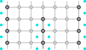
Figure 4.1. The boundary faces with reduced weight are marked. The marked faces next to the slit are virtual faces accessed across the slit from an interior face.

Refinements to the lattice domains

Since we use discrete complex analysis only in the lattice strip ${{\mathbb{S}}^{(0pt)}}$ and lattice slit-strip ${{\mathbb{S}}_{\mathrm{slit}}^{(0pt)}}$, we will present the tools in the simplest form that applies to these cases. Moreover, since our main objective is to show convergence results in the scaling limit framework, where the lattice variables are rescaled by a factor $0pt^{-1}$, we will present the key notions in the context of the rescaled square lattice $\delta\mathbb{Z}^{2}$ for $\delta>0$: the choice $\delta=1$ corresponds to the original lattice setup, and the choice $\delta=0pt^{-1}$ will be used for scaling limit results.

The following graph notations will be needed. We denote the set of vertices by $\mathrm{V}=\delta\,{{\mathbb{S}}^{(0pt)}}=\delta\,{{\mathbb{S}}_{\mathrm{slit}}^{(0pt)}}$, and the set of edges by $\mathrm{E}$; so $\mathrm{E}=\delta\mathrm{E}({{\mathbb{S}}^{(0pt)}})$ or $\mathrm{E}=\delta\mathrm{E}({{\mathbb{S}}_{\mathrm{slit}}^{(0pt)}})$. We moreover use the notation $\mathrm{V}^{*}$ for the set of faces. The “imaginary part of the integral of the square” will be defined on $\mathrm{V}\cup\mathrm{V}^{*}$. For the treatment of boundary values, we also introduce boundary faces, which are imagined faces across the boundary edges as in Figure 4.1. The set of boundary faces is denoted by $\partial\mathrm{V}^{*}$, and it is by definition in bijective correspondence with the set of boundary edges.

Let us also define a corner of our graph to be a pair $c=(v,p)$ consisting of a vertex $v\in\mathrm{V}$ and a face $p\in\mathrm{V}^{*}$ which are adjacent to each other.

S-holomophicity and the imaginary part of the integral of the square

The definition (3.6) of s-holomorphicity of a function $F\colon\mathrm{E}\to\mathbb{C}$ can be reinterpreted as follows. For any corner $c=(v,p)$, the values $F(z_{1})$ and $F(z_{2})$ on both edges $z_{1},z_{2}\in\mathrm{E}$ adjacent to $v$ and $p$ have the same projection to the line $\sqrt{\mathbbm{i}/(v-p)}\,\mathbb{R}$ in the complex plane, i.e., we may associate a well-defined value to the function $F$ at the corner $c=(v,p)$ by

$$F(c):=\; \mathrm{pr}_{\sqrt{\mathbbm{i}/(v-p)}\,\mathbb{R}}\big{(}F(z_{j})\big{)}\,=\,\frac{1}{2}\Big{(}F(z_{j})+\frac{\mathbbm{i}\,|v-p|}{v-p}\,\overline{F(z_{j})}\Big{)},\qquad\text{ for $j=1,2$.}$$

For any s-holomophic function

$$F\colon\mathrm{E}\to\mathbb{C}$$

there exists a function

$$H\colon\mathrm{V}\cup\mathrm{V}^{*}\to\mathbb{R},$$

defined uniquely up to an additive real constant by the condition that for any vertex $v$ and adjacent face $p$, with $c=(v,p)$ the associated corner, we have

(4.3) $$H(v)-H(p):=\; \Im\mathfrak{m}\Big{(}2\,F(c)^{2}\;(v-p)\Big{)}=\sqrt{2}\,\delta\,\left|F(c)\right|^{2}\geq 0;$$

see [ChSm12, Proposition 3.6(i)]. The factor two in front of the squared value is included because of the definition of the values on corners: if $u,u^{\prime}$ are two adjacent vertices of faces and $z=\frac{u+u^{\prime}}{2}\in\mathrm{E}$ the edge between them, then a calculation [ChSm12, Proposition 3.6(ii)] from (4.3) shows

(4.4) $$H(u^{\prime})-H(u)=\; \Im\mathfrak{m}\Big{(}F(z)^{2}\;(u^{\prime}-u)\Big{)}.$$

We denote

$$H=\Im\mathfrak{m}\left(\int_{\times}{F}^{2}\right),$$

and call $H$ the “imaginary part of the integral of the square” of $F$. Note that from the definition (4.3) it is clear that for a vertex $v\in\mathrm{V}$ and an adjacent face $p\in\mathrm{V}^{*}$, we always have $H(v)\geq H(p)$.

When $F$ has Riemann boundary value (3.7) on a boundary edge $z$ between adjacent boundary vertices $v,v^{\prime}$, we see from (4.4) that $H(v)=H(v^{\prime})$. Therefore Riemann boundary values for an s-holomorphic function $F$ imply that $H=\Im\mathfrak{m}\left(\int_{\times}{F}^{2}\right)$ is constant on the boundary vertices of each boundary part. We then extend the definition to the boundary faces by the same constant, and obtain a function

$$H\colon\mathrm{V}\cup\mathrm{V}^{*}\cup\partial\mathrm{V}^{*}\to\mathbb{R}.$$

4.3. Sub- and superharmonicity and the maximum principle

Unlike in the continuous case, the “imaginary part of the integral of the square” $H=\Im\mathfrak{m}\left(\int_{\times}{F}^{2}\right)$ of an s-holomorphic function $F$ is not (discrete) harmonic. The remarkable observation is that it nevertheless mimics the behavior of harmonic functions extremely well: its restriction $H|_{\mathrm{V}}$ to vertices is superharmonic, and its restriction $H|_{\mathrm{V}^{*}}$ to faces is subharmonic, and because of the boundary values, the values on vertices and faces are suitably close. The first incarnation of this almost harmonicity of $H$ is the following version of the maximum principle.

Lemma 4.4 ([ChSm12, Proposition 3.6(iii) and Lemma 3.14]).

Let $F\colon\mathrm{E}\to\mathbb{C}$ be s-holomorphic with Riemann boundary values, and let $H=\Im\mathfrak{m}\left(\int_{\times}{F}^{2}\right)$, ${H\colon\mathrm{V}\cup\mathrm{V}^{*}\cup\partial\mathrm{V}^{*}\to\mathbb{R}}$ be defined as above. Then we have:

• At any interior vertex $v$, the value of $H$ is at most the simple arithmetic average of the values at the four neighboring vertices,

  $$H(v)\leq\frac{1}{4}\Big{(}H(v+\delta)+H(v+\mathbbm{i}\delta)+H(v-\delta)+H(v-\mathbbm{i}\delta)\Big{)}.$$

  In particular $H$ can not have a strict local maximum at an interior vertex.

• At any interior face $p$, the value of $H$ is at least the weighted average of the values at the four neighboring faces,

  $$H(p)\geq\frac{\sum_{s\in\left\{\delta,\mathbbm{i}\delta,-\delta,-\mathbbm{i}\delta\right\}}\mathbf{w}(p+s)\,H(p+s)}{\sum_{s\in\left\{\delta,\mathbbm{i}\delta,-\delta,-\mathbbm{i}\delta\right\}}\mathbf{w}(p+s)},$$

  where $\mathbf{w}(p^{\prime})=1$ for $p^{\prime}\in\mathrm{V}^{*}$, and $\mathbf{w}(p^{\prime})=2(\sqrt{2}-1)$ for $p^{\prime}\in\partial\mathrm{V}^{*}$. In particular $H$ can not have a strict local minimum at an interior face.

With this version of the maximum principle we can give the proof of Lemma 3.8: If a function $f\in\mathscr{F}^{(0pt)}$ admits regular extensions to the top, to the left leg, and to the right leg, then $f\equiv 0$.

Proof of Lemma 3.8.

Suppose $f\in\mathscr{F}^{(0pt)}$ admits regular extensions to all three extremities of the slit-strip.

Consider the s-holomorphic extension $F\colon\mathrm{E}({{\mathbb{S}}_{\mathrm{slit}}^{(0pt)}})\to\mathbb{C}$ of $f$ to the lattice slit-strip, with Riemann boundary values. The regular extensions assumption implies that $F$ decays exponentially in all three extremities: the norm of its restrictions to horizontal cross-sections decreases by at least a factor $\Lambda_{-1/2}^{(0pt)}<1$ (resp. $\max\{\Lambda_{-1/2}^{(\ell^{\mathrm{L}})},\Lambda_{-1/2}^{(\ell^{\mathrm{R}})}\}<1$) on each vertical step in the upwards direction (resp. downwards direction). It follows that on horizontal lines in the top part, the differences of all values of $H=\Im\mathfrak{m}\left(\int_{\times}{F}^{2}\right)$ to the boundary values tend to zero:

$$\begin{cases}\max_{x\in I^{*}}\big{|}H(x+\mathbbm{i}y)-H(a+\mathbbm{i}y)\big{|}\to 0\\ \max_{x\in I^{*}}\big{|}H(x+\mathbbm{i}y)-H(b+\mathbbm{i}y)\big{|}\to 0\end{cases}\qquad\text{ as $y\to+\infty$.}$$

Recalling that the boundary values $H(a+\mathbbm{i}y),H(b+\mathbbm{i}y)$ are constant (independent of $y$), it follows first of all that the values on the two boundaries are equal, ${H(a+\mathbbm{i}y)=H(b+\mathbbm{i}y)=:M}$, and furthermore that $H(x+\mathbbm{i}y)$ approaches these boundary values $M$ as $y\to+\infty$. Similarly, the values in the horizontal cross-sections of the left and right legs are tending to the same constant $M$, and in particular the boundary values on the slit part are also equal to $M$.

It then follows from the maximum principle on vertices, Lemma 4.4(i), that $H|_{\mathrm{V}}\leq M$. Similarly by the minimum principle on faces, Lemma 4.4(ii), we get $H|_{\mathrm{V}^{*}}\geq M$. But as the values on vertices are at least the values on adjacent faces, we get $H\equiv M$. We thus conclude that $F\equiv 0$ and in particular $f\equiv 0$. ∎

4.4. Convergence of the distinguished functions in the slit-strip

Besides the maximum principle, we need more quantitative tools of the regularity theory of s-holomorphic functions to prove the scaling limit result for the distinguished functions in the slit-strip.

Beurling-type estimates

We will need the following weak Beurling-type estimates (meaning that the exponent $\beta$ does not have to be optimal) for discrete harmonic measures on vertices and faces from [ChSm11].

Proposition 4.5 ([ChSm11, Proposition 2.11]).

There exists absolute constants ${\beta,\mathrm{const.}>0}$ such that the following holds. Let $\partial\mathrm{V}$ denote the set of boundary vertices, and $\partial\mathrm{V}_{0}\subset\partial\mathrm{V}$ a subset. Then the discrete harmonic function $\omega_{\circ}\colon\mathrm{V}\to[0,1]$ on vertices, with boundary values $0$ on $\partial\mathrm{V}_{0}$ and $1$ on $\partial\mathrm{V}\setminus\partial\mathrm{V}_{0}$, satisfies

$$\omega_{\circ}(v)\leq\mathrm{const.}\cdot\Big{(}\frac{\mathrm{dist}(v,\;\partial\mathrm{V})}{\mathrm{dist}(v,\;\partial\mathrm{V}\setminus\partial\mathrm{V}_{0})}\Big{)}^{\beta}.$$

Similarly, let $\partial\mathrm{V}^{*}$ denote the set of boundary faces, and $\partial\mathrm{V}^{*}_{0}\subset\partial\mathrm{V}^{*}$ a subset. Then the discrete harmonic function (w.r.t. modified boundary face weights as in Lemma 4.4) $\omega_{\bullet}\colon\mathrm{V}^{*}\to[0,1]$ on faces with boundary values $0$ on $\partial\mathrm{V}^{*}_{0}$ and $1$ on $\partial\mathrm{V}^{*}\setminus\partial\mathrm{V}^{*}_{0}$, satisfies

$$\omega_{\bullet}(p)\leq\mathrm{const.}\cdot\Big{(}\frac{\mathrm{dist}(p,\;\partial\mathrm{V}^{*})}{\mathrm{dist}(p,\;\partial\mathrm{V}^{*}\setminus\partial\mathrm{V}^{*}_{0})}\Big{)}^{\beta}.$$

Precompactness estimates

The following result from [ChSm12] yields uniform boundedness and equicontinuity (i.e., precompactness in the Arzelà-Ascoli sense) for both $F$ and $H$, given control on $|H|$.

Theorem 4.6 ([ChSm12, Theorem 3.12]).

There exists absolute constants (independent of lattice mesh $\delta$ and lattice domains) such that the following estimates hold. Let $F\colon\mathrm{E}\to\mathbb{C}$ be s-holomorphic with Riemann boundary values, and let $H=\Im\mathfrak{m}\left(\int_{\times}{F}^{2}\right)$, $H\colon\mathrm{V}\cup\mathrm{V}^{*}\to\mathbb{R}$ be defined as above. Suppose that the ball $B_{r}(x_{0})$, with $r\geq\mathrm{const.}\cdot\delta$, is contained in the lattice domain and does not intersect its boundary. Then for $z,z^{\prime}\in\mathrm{E}$ adjacent edges contained in the smaller ball $B_{r/2}(x_{0})$, we have

(4.5) $$\left|F(z)\right|\leq\; \mathrm{const.}\cdot\sqrt{\frac{\max_{B_{r}(x_{0})}\left|H\right|}{r}},$$

$$\frac{\left|F(z^{\prime})-F(z)\right|}{\delta}\leq\; \mathrm{const.}\cdot\sqrt{\frac{\max_{B_{r}(x_{0})}\left|H\right|}{r^{3}}}.$$

Limit result for the slit-strip functions

With the above tools, we can prove the scaling limit result for the pole functions.

Theorem 4.7.

Choose sequences $(a_{n})_{n\in\mathbb{N}}$, $(b_{n})_{n\in\mathbb{N}}$ of integers $a_{n},b_{n}\in\mathbb{Z}$ such that

• $a_{n}<0<b_{n}$ for all $n$;

• $0pt_{n}:=b_{n}-a_{n}\to+\infty$ as $n\to\infty$;

• $a_{n}/0pt_{n}\to-\frac{1}{2}$ and $b_{n}/0pt_{n}\to+\frac{1}{2}$ as $n\to\infty$.

For $k\in\mathcal{K}$, let $\mathfrak{P}_{\mathrm{T};k}^{(0pt_{n})},\mathfrak{P}_{\mathrm{L};k}^{(0pt_{n})},\mathfrak{P}_{\mathrm{R};k}^{(0pt_{n})}$ denote the functions of Section 3.4 in the lattice strips with $a=a_{n}$ and $b=b_{n}$, and let ${P}^{\mathrm{T}}_{k},{P}^{\mathrm{L}}_{k},{P}^{\mathrm{R}}_{k}\colon{\mathbb{S}}_{\mathrm{slit}}\to\mathbb{C}$ denote the pure pole functions of Proposition 2.6. Then, as $n\to\infty$, we have

$$\sqrt{0pt_{n}}\;\mathfrak{P}_{\mathrm{T};k}^{(0pt_{n})}\big{(}z0pt_{n}\big{)}\to\; {P}^{\mathrm{T}}_{k}(z) {\mathbb{S}}_{\mathrm{slit}}\ni z$$ uniformly on compact subsets of 

$$\sqrt{0pt_{n}}\;\mathfrak{P}_{\mathrm{L};k}^{(0pt_{n})}\big{(}z0pt_{n}\big{)}\to\; {P}^{\mathrm{L}}_{k}(z) {\mathbb{S}}_{\mathrm{slit}}\ni z$$ uniformly on compact subsets of 

$$\sqrt{0pt_{n}}\;\mathfrak{P}_{\mathrm{R};k}^{(0pt_{n})}\big{(}z0pt_{n}\big{)}\to\; {P}^{\mathrm{R}}_{k}(z) \text{ uniformly on compact subsets of\leavevmode\nobreak\ ${\mathbb{S}}_{\mathrm{slit}}\ni z$}.$$

Proof.

Let us consider the convergence of the left leg pole functions — the other cases are similar. Including the rescalings in the definition, let us define functions $F^{(n)}$ on $\frac{1}{0pt_{n}}{{\mathbb{S}}_{\mathrm{slit}}^{(0pt_{n})}}$ by the formula $F^{(n)}(z)=\sqrt{0pt_{n}}\;\mathfrak{P}_{\mathrm{L};k}^{(0pt_{n})}\big{(}z0pt_{n}\big{)}$. Define also $H^{(n)}=\Im\mathfrak{m}\left(\int_{\times}{F^{(n)}}^{2}\right)$, with the additive constant chosen so that this function vanishes at the tip of the slit, $H^{(n)}(0)=0$. Then $H^{(n)}$ vanishes on the entire slit (it is constant on boundary components), and since $F^{(n)}$ decays exponentially in the top and the right leg extremities, the same argument as in the proof of Lemma 3.8 shows that the boundary values of $H^{(n)}$ also on the left and right boundaries are zero, and that $H^{(n)}$ tends to zero in the top and right extremities.

For $K>0$, consider a horizontal cross-cut $L_{K}^{(n)}$ of the left leg of $\frac{1}{0pt_{n}}{{\mathbb{S}}_{\mathrm{slit}}^{(0pt_{n})}}$ at imaginary part $-K$ (more precisely, the horizontal line of the lattice $\frac{1}{0pt_{n}}{{\mathbb{S}}_{\mathrm{slit}}^{(0pt_{n})}}$ with largest imaginary part below $-K$), and consider the truncated slit-strip $S_{K}^{(n)}\subset\frac{1}{0pt_{n}}{{\mathbb{S}}_{\mathrm{slit}}^{(0pt_{n})}}$ defined as the component of the complement of this cross-section which contains the top and right extremities. Define $M^{(n)}_{K}:=\max_{L_{K}^{(n)}}\big{|}H^{(n)}\big{|}$, where $L_{K}^{(n)}$ is interpreted to consist of both the vertices on the horizontal line and the faces just below that horizontal line. By the maximum principle, Lemma 4.4, we have $M^{(n)}_{K}=\max_{S_{K}^{(n)}}\big{|}H^{(n)}\big{|}$, so in view of $S_{K}^{(n)}\subset S_{K^{\prime}}^{(n)}$ for $K<K^{\prime}$ we have that $M^{(n)}_{K}$ is increasing in $K$.

We will later prove that for any $K>0$, the sequence $(M^{(n)}_{K})_{n\in\mathbb{N}}$ is bounded, i.e., we have $M_{K}:=\sup_{n\in\mathbb{N}}M^{(n)}_{K}<\infty$. We now first prove the convergence of $F^{(n)}$ to ${P}^{\mathrm{L}}_{k}$ assuming this. Denote by $L_{K}$ the horizontal cross-cut of the left leg of the continuum slit-strip ${\mathbb{S}}_{\mathrm{slit}}$ at imaginary part $-K$, and by $S_{K}\subset{\mathbb{S}}_{\mathrm{slit}}$ the component of ${\mathbb{S}}_{\mathrm{slit}}\setminus L_{K}$ which contains the top and right extremities. Then by the boundedness of $(M^{(n)}_{K})_{n\in\mathbb{N}}$, the functions $H^{(n)}$ restricted to the part $S_{K}$ are uniformly bounded, and therefore as a consequence of Theorem 4.6, both $H^{(n)}$ and $F^{(n)}$ are equicontinuous and uniformly bounded on compact subsets of $S_{K}$. By the Arzelà-Ascoli theorem, along a subsequence we have uniform convergence of $H^{(n)}$ and $F^{(n)}$ on compact subsets of $S_{K}$, and since this holds for any $K>0$, by diagonal extraction there exists a subsequence along which $H^{(n)}$ and $F^{(n)}$ converge uniformly on compact subsets of the whole slit-strip ${\mathbb{S}}_{\mathrm{slit}}$. We must show that in any such subsequential limit $(H,F)$ we in fact have $F={P}^{\mathrm{L}}_{k}$.

Note that in such a subsequential limit we have $H=\Im\mathfrak{m}\Big{(}\int F(z)^{2}\,\mathrm{d}z\Big{)}$, and as a locally uniform limit of both subharmonic and superharmonic functions ($H^{(n)}$ on vertices and faces), $H$ is harmonic. It follows that $F^{2}=2\mathbbm{i}\,\partial_{z}H$ is holomorphic, and thus $F$ is also holomorphic. By Lemma 4.4, $H^{(n)}$ is bounded above by $M_{K}\,\omega_{\circ}^{(n)}$, where $\omega_{\circ}^{(n)}$ is the discrete harmonic measure on the vertices of $S_{K}^{(n)}$ of the cross-cut $L_{K}^{(n)}$. Similarly $H^{(n)}$ is bounded below by $-M_{K}\,\omega_{\bullet}^{(n)}$, where $\omega_{\bullet}^{(n)}$ is the discrete harmonic measure on the faces of $S_{K}^{(n)}$ just below the cross-cut $L_{K}^{(n)}$ (with the modified boundary weights). By Beurling estimates, Proposition 4.5, these harmonic measures decay at the top and right extremities uniformly in $n$, so the subsequential limit $H$ of the $H^{(n)}$ decays at the at the top and right extremities. On $S_{K-\varepsilon}$, for any $\varepsilon>0$, these harmonic measures also decay uniformly upon approaching the boundaries of the slit-strip, again by virtue of the Beurling estimates. We conclude that $H$ also tends to zero on the boundary. Then also $F$ decays at top and right extremities, by Theorem 4.6, and $F$ has Riemann boundary values by [ChSm12, Remark 6.3]. In order to conclude that $F={P}^{\mathrm{L}}_{k}$, it remains to show that $F-E^{\mathrm{L}}_{-k}$ decays in the left leg extremity.

By definition of the discrete pole function $\mathfrak{P}_{\mathrm{L};k}$, in the left leg we can write

$$F^{(n)}(z)=F_{0}^{(n)}(z)+\sqrt{0pt_{n}}\,\mathfrak{F}_{\mathrm{L};-k}(z0pt_{n}),$$

where $F_{0}^{(n)}$ decays in the left leg extremity. From Theorem 4.3, we already know that the second term on the right hand side above converges to $E^{\mathrm{L}}_{-k}$, uniformly on compact subsets. To control $F_{0}^{(n)}$, consider $H_{0}^{(n)}=\Im\mathfrak{m}\left(\int_{\times}{F_{0}^{(n)}}^{2}\right)$. By similar arguments as above for $H^{(n)}$, one shows that one can extract subsequences from $(H_{0}^{(n)},F_{0}^{(n)})$ which converge uniformly on compacts in the left leg, and that for any subsequential limit $(H_{0},F_{0})$ we have that $F_{0}$ decays in the left leg extremity. But such an $F_{0}(z)$ is, as the limit of $F^{(n)}(z)-\sqrt{0pt_{n}}\,\mathfrak{F}_{\mathrm{L};-k}(z0pt_{n})$, equal to $F(z)-E^{\mathrm{L}}_{-k}(z)$. We have thus seen that $F$ is holomorphic with Riemann boundary values in the slit-strip, $F$ decays at the top and right leg extremities, and $F-E^{\mathrm{L}}_{-k}$ decays at the left leg extremity. We conclude that $F={P}^{\mathrm{L}}_{k}$.

To finish the proof, we must still show the boundedness of $(M^{(n)}_{K})_{n\in\mathbb{N}}$. Suppose that instead $M^{(n)}_{K}\to\infty$ along some subsequence, for some $K>0$ and therefore by monotonicity for all large enough $K$. Now $(M^{(n)}_{K})^{-1}\,\big{|}H^{(n)}\big{|}$ is bounded by $1$ on $L_{K}^{(n)}$, and by selecting a large enough $K$ we get by Beurling estimates as before that $(M^{(n)}_{K})^{-1}\,\big{|}H^{(n)}\big{|}\leq\frac{1}{5}$ on $L_{0}^{(n)}$. Again decompose $F^{(n)}(z)=F_{0}^{(n)}(z)+\sqrt{0pt_{n}}\,\mathfrak{F}_{\mathrm{L};-k}(z0pt_{n})$ in the left leg, and denote by $H_{0}^{(n)}$ the imaginary part of the integral of the square of $F_{0}^{(n)}$. Noting that as $n\to\infty$ along the subsequence, we have $(M^{(n)}_{K})^{-1/2}\,\sqrt{0pt_{n}}\,\big{|}\mathfrak{F}_{\mathrm{L};-k}(z0pt_{n})\big{|}\to 0$ uniformly on $S_{K+1}\ni z$, we see that $(M^{(n)}_{K})^{-1}\,\big{|}H_{0}^{(n)}\big{|}\leq\frac{2}{5}$ on $L_{0}^{(n)}$ for large enough $n$. By the decay in the left leg and the maximum principle, $H_{0}^{(n)}$ is bounded by its values on $L_{0}^{(n)}$, so $(M^{(n)}_{K})^{-1}\,\big{|}H_{0}^{(n)}\big{|}\leq\frac{2}{5}$ everywhere. But similarly by the smallness of $(M^{(n)}_{K})^{-1/2}\,\sqrt{0pt_{n}}\,\big{|}\mathfrak{F}_{\mathrm{L};-k}(z0pt_{n})\big{|}$ on $S_{K+1}\ni z$, we see that the difference $H^{(n)}-H_{0}^{(n)}$ is small, to that in particular $(M^{(n)}_{K})^{-1}\,\big{|}H^{(n)}\big{|}\leq\frac{3}{5}$ on $L_{K}^{(n)}$, for large $n$ in the subsequence. This is a contradiction with the definition of $M^{(n)}_{K}$, so indeed $(M^{(n)}_{K})_{n\in\mathbb{N}}$ had to be bounded and the proof is complete. ∎

Convergence of inner products

For applications to the convergence of the Ising model fusion coefficients, it is not enough for us to have the uniform convergence on compacts of the distinguished discrete functions to the distinguished continuum ones. We need the convergence of the inner products of their restrictions to the cross-section as well.

Corollary 4.8.

Choose sequences $(a_{n})_{n\in\mathbb{N}}$, $(b_{n})_{n\in\mathbb{N}}$ of integers $a_{n},b_{n}\in\mathbb{Z}$ such that

• $a_{n}<0<b_{n}$ for all $n$;

• $0pt_{n}:=b_{n}-a_{n}\to+\infty$ as $n\to\infty$;

• $a_{n}/0pt_{n}\to-\frac{1}{2}$ and $b_{n}/0pt_{n}\to+\frac{1}{2}$ as $n\to\infty$.

For $k\in\mathcal{K}$, let

$$\mathfrak{p}_{\mathrm{T};k}^{(0pt_{n})},\;\mathfrak{p}_{\mathrm{L};k}^{(0pt_{n})},\;\mathfrak{p}_{\mathrm{R};k}^{(0pt_{n})},\;\mathfrak{f}_{\pm k}^{(0pt_{n})},\;\mathfrak{f}_{\mathrm{L};\pm k}^{(0pt_{n})},\;\mathfrak{f}_{\mathrm{R};\pm k}^{(0pt_{n})}\;\in\;\mathscr{F}^{(0pt_{n})}$$

denote the functions defined before in the lattice strips with $a=a_{n}$ and $b=b_{n}$. Correspondingly, let

$${p}^{\mathrm{T}}_{k},\;{p}^{\mathrm{L}}_{k},\;{p}^{\mathrm{R}}_{k},\;e_{\pm k},\;e^{\mathrm{L}}_{\pm k},\;e^{\mathrm{R}}_{\pm k}\;\in\;\mathscr{L}^{2}$$

be the continuum functions defined before.

Then as $n\to\infty$, we have the convergence of all inner products in $\mathscr{F}^{(0pt_{n})}$ to the corresponding ones in $\mathscr{L}^{2}$:

$$\langle\mathfrak{f}_{{\star};k}^{(0pt_{n})},\mathfrak{f}_{{\star^{\prime}};k^{\prime}}^{(0pt_{n})}\rangle\to\; \langle e^{{\star}}_{k},e^{{\star^{\prime}}}_{k^{\prime}}\rangle \star,\star^{\prime}\in\left\{\mathrm{T},\mathrm{L},\mathrm{R}\right\} k,k^{\prime}\in\pm\mathcal{K}$$ for and ,

$$\langle\mathfrak{p}_{{\star};k}^{(0pt_{n})},\mathfrak{f}_{{\star^{\prime}};k^{\prime}}^{(0pt_{n})}\rangle\to\; \langle{p}^{{\star}}_{k},e^{{\star^{\prime}}}_{k^{\prime}}\rangle \star,\star^{\prime}\in\left\{\mathrm{T},\mathrm{L},\mathrm{R}\right\} k\in\mathcal{K} k^{\prime}\in\pm\mathcal{K}$$ for and , ,

$$\langle\mathfrak{p}_{{\star};k}^{(0pt_{n})},\mathfrak{p}_{{\star^{\prime}};k^{\prime}}^{(0pt_{n})}\rangle\to\; \langle{p}^{{\star}}_{k},{p}^{{\star^{\prime}}}_{k^{\prime}}\rangle \star,\star^{\prime}\in\left\{\mathrm{T},\mathrm{L},\mathrm{R}\right\} k,k^{\prime}\in\mathcal{K}$$ for and

(where the hitherto undefined notations are interpreted so that $\mathfrak{f}_{\mathrm{T};k}=\mathfrak{f}_{k}$ and $e^{\mathrm{T}}_{k}=e_{k}$).

Proof.

The proofs of all cases are similar, so we will only consider in detail a typical one,

$$\langle\mathfrak{p}_{\mathrm{L};k},\mathfrak{f}_{k^{\prime}}\rangle\to\langle{p}^{\mathrm{L}}_{k},e_{k^{\prime}}\rangle.$$

We again work in the rescaled slit-strip $\frac{1}{0pt_{n}}{{\mathbb{S}}_{\mathrm{slit}}^{(0pt)}}$, and now use the functions $x\mapsto\sqrt{0pt_{n}}\,\mathfrak{p}_{\mathrm{L};k}^{(0pt_{n})}(x0pt_{n})$, ${x\mapsto{\sqrt{0pt_{n}}\,\mathfrak{f}_{k^{\prime}}^{(0pt_{n})}(x0pt_{n})}}$ with piecewise constant interpolation for convenience (by the equicontinuity estimates, this does not change the convergence statements). The discrete inner product can be written as the integral of the piecewise constant interpolation

$$\langle\mathfrak{p}_{\mathrm{L};k}^{(0pt_{n})},\mathfrak{f}_{k^{\prime}}^{(0pt_{n})}\rangle=\; \Re\mathfrak{e}\left(\sum_{x^{\prime}\in\llbracket a_{n},b_{n}\rrbracket^{*}}\mathfrak{p}_{\mathrm{L};k}^{(0pt_{n})}(x^{\prime})\;\overline{\mathfrak{f}_{k^{\prime}}^{(0pt_{n})}(x^{\prime})}\right)$$

$$=\; \Re\mathfrak{e}\left(\int_{a_{n}/0pt_{n}}^{b_{n}/0pt_{n}}\sqrt{0pt_{n}}\,\mathfrak{p}_{\mathrm{L};k}^{(0pt_{n})}(x0pt_{n})\;\overline{\sqrt{0pt_{n}}\,\mathfrak{f}_{k^{\prime}}^{(0pt_{n})}(x0pt_{n})}\;\mathrm{d}x\right).$$

For small $\epsilon>0$, let $\mathcal{I}^{\epsilon}:=[-\frac{1}{2}+\epsilon,-\epsilon]\cup[\epsilon,\frac{1}{2}-\epsilon]$. By Theorem 4.3, we have

$$\sqrt{0pt_{n}}\,\mathfrak{f}_{k^{\prime}}^{(0pt_{n})}(x0pt_{n})\to\; e_{k^{\prime}}(x) \mathcal{I}=\Big{[}-\frac{1}{2},\frac{1}{2}\Big{]}\ni x$$ uniformly on ,

and by Theorem 4.7, we have

$$\sqrt{0pt_{n}}\,\mathfrak{p}_{\mathrm{L};k}^{(0pt_{n})}(x0pt_{n})\to\; {p}^{\mathrm{L}}_{k}(x) \mathcal{I}^{\epsilon}\ni x$$ uniformly on .

Comparing the discrete inner product with the continuum inner product

$$\langle{p}^{\mathrm{L}}_{k},e_{k^{\prime}}\rangle=\; \Re\mathfrak{e}\left(\int_{-1/2}^{+1/2}{p}^{\mathrm{L}}_{k}(x)\;\overline{e_{k^{\prime}}(x)}\;\mathrm{d}x\right)$$

the uniform convergence shows that the contributions to the integrals from $\mathcal{I}^{\varepsilon}$ converge to the desired ones for any $\epsilon>0$, and it remains to show that the contributions from within distance $\epsilon$ to the points $-\frac{1}{2},0,\frac{1}{2}$ are negligible in the limit $\epsilon\to 0$.

Note that $|e_{k^{\prime}}(x)|\leq 1$ for all $x\in\mathcal{I}$, and its discrete counterpart $\sqrt{0pt_{n}}\,\mathfrak{f}_{k^{\prime}}^{(0pt_{n})}(x0pt_{n})$ is bounded by an absolute constant, too. It therefore remains to control the discrete pole functions $\sqrt{0pt_{n}}\;\mathfrak{p}_{\mathrm{L};k}^{(0pt_{n})}\big{(}x0pt_{n}\big{)}$ and their continuous counterparts. But in the proof of Theorem 4.7 we saw by Beurling estimates that the imaginary part of the integral of the square $H^{(n)}=\Im\mathfrak{m}\left(\int_{\times}{F^{(n)}}^{2}\right)$ of the pole function $F^{(n)}(z)=\sqrt{0pt_{n}}\;\mathfrak{P}_{\mathrm{L};k}^{(0pt_{n})}\big{(}z0pt_{n}\big{)}$ tends to zero near the boundaries. Combined with (4.5), we get $\big{|}\sqrt{0pt_{n}}\;\mathfrak{p}_{\mathrm{L};k}^{(0pt_{n})}\big{(}x0pt_{n}\big{)}\big{|}=\mathcal{O}(|x-c|^{(\beta-1)/2})$ for $c\in\left\{-\frac{1}{2},0,\frac{1}{2}\right\}$. With these estimates of the two types of functions to be integrated, we see that the contribution to the integrals from within distance $\epsilon$ to the points $-\frac{1}{2},0,\frac{1}{2}$ is in this case $\mathcal{O}(\epsilon^{(1+\beta)/2})$. This proves the desired convergence $\langle\mathfrak{p}_{\mathrm{L};k},\mathfrak{f}_{k^{\prime}}\rangle\to\langle{p}^{\mathrm{L}}_{k},e_{k^{\prime}}\rangle$.

Note that among the many cases in the statement, the above type of reasoning results in the worst bounds for two pole type functions (no a priori bounds besides the Beurling estimates are available for either factors). But even in that case the product in the integrand is $\mathcal{O}(|x-c|^{\beta-1})$ for $c\in\left\{-\frac{1}{2},0,\frac{1}{2}\right\}$, and the contributions to the integrals from within distance $\epsilon$ to the points $-\frac{1}{2},0,\frac{1}{2}$ are $\mathcal{O}(\epsilon^{\beta})$ as $\epsilon\to 0$, which is sufficient for the convergence of the inner products. ∎

Acknowledgments: S.P. is supported by a KIAS Individual Grant (MG077201) at Korea Institute for Advanced Study. T.A. was affiliated with the Department of Mathematics and Statistics at the American University of Sharjah, and recognizes their financial support.

References

- [AbMa73] D. B. Abraham and A. Martin-Löf. The Transfer Matrix for a Pure Phase in the Two-dimensional Ising Model. Comm. Math. Phys., 1973, 32, 245-268
- [AKP21] T. Ameen, K. Kytölä, and S. C. Park. Slit-strip Ising boundary conformal field theory 2: Scaling limits of fusion coefficients. Preprint: https://arxiv.org/abs/2108.05105, 2021.
- [Bax82] R. J. Baxter. Exactly solved models in statistical mechanics. Academic Press, 1982.
- [BaEn78] R. J. Baxter and I. G. Enting. 399th solution of the Ising model. J. Phys. A: Math. Gen. 11, 1978.
- [BPW18] V. Beffara, E. Peltola, and H. Wu. On the uniqueness of global multiple SLEs, https://arxiv.org/pdf/1801.07699, 2018.
- [BPZ84a] A. A. Belavin, A. M. Polyakov, and A. B. Zamolodchikov. Infinite conformal symmetry in two-dimensional quantum field theory. Nucl. Phys. B, 241(2):333–380, 1984.
- [BPZ84b] A. A. Belavin, A. M. Polyakov, and A. B. Zamolodchikov. Infinite conformal symmetry of critical fluctuations in two dimensions. J. Stat. Phys., 34(5-6):763–774, 1984.
- [BeHo19] S. Benoist and C. Hongler. The scaling limit of critical Ising interfaces is CLE(3). Ann. Probab. 47:2049–2086, 2019.
- [BDH16] S. Benoist H. Duminil-Copin, and C. Hongler. Conformal invariance of crossing probabilities for the Ising model with free boundary conditions. Ann. Inst. H. Poincaré Probab. Statist. 52:1784–1798, 2016.
- [CGN15] F. Camia, C. Garban, and C. M. Newman. Planar Ising magnetization field I. Uniqueness of the critical scaling limit. Ann. Probab. 43:528–571, 2015.
- [CGN16] F. Camia, C. Garban, and C. M. Newman. Planar Ising magnetization field II. Properties of the critical and near-critical scaling limits. Ann. Inst. Henri Poincarᅵ, Probab. Stat., 2016, 52, 146-161
- [Che18] D. Chelkak. Planar Ising model at criticality: state-of-the-art and perspectives. Proceedings of the International Congress of Mathematicians 2018 3:2789–2816. World Scientific Publishing Company Inc., 2018.
- [CCK17] D. Chelkak, D. Cimasoni, and A. Kassel. Revisiting the combinatorics of the 2D Ising model. Ann. Inst. Henri Poincaré (D) 4(3):309–385, 2017.
- [CDHKS14] D. Chelkak, H. Duminil-Copin, C. Hongler, A. Kemppainen, and S. Smirnov. Convergence of Ising interfaces to Schramm’s SLE curves. C. R. Acad. Sci. Paris Ser. I 352:157–161, 2014.
- [CHI15] D. Chelkak, C. Hongler, and K. Izyurov. Conformal invariance of spin correlations in the planar Ising model. Annals of Math., 181(3):1087–1138, 2015.
- [CHI21] D. Chelkak, C. Hongler, and K. Izyurov. Correlations of primary fields in the critical Ising model. Preprint https://arxiv.org/abs/2103.10263, 2021.
- [ChIz13] D. Chelkak and K. Izyurov. Holomorphic Spinor Observables in the Critical Ising Model. Comm. Math. Phys. 322:303–332, 2013.
- [ChSm11] D. Chelkak and S. Smirnov. Discrete complex analysis on isoradial graphs. Advances in Mathematics, 228:1590–1630, 2011.
- [ChSm12] D. Chelkak, S. Smirnov. Universality in the 2D Ising model and conformal invariance of fermionic observables. Invent math., 189(3):515–580, 2012.
- [DIK13] P. Deift, A. Its, and I. Krasovsky. Toeplitz matrices and Toeplitz determinants under the impetus of the Ising model. Some history and some recent results Comm. Pure Appl. Math. 66:1360–1438, 2013.
- [DMS97] P. Di Francesco, P. Mathieu and D. Sénéchal. Conformal Field Theory. Graduate texts in contemporary physics. Springer-Verlag New York, 1997.
- [Dub11] J. Dubédat. Exact bosonizboson of the Ising model. https://arxiv.org/abs/1112.4399, 2011.
- [Fis66] M. E. Fisher. On the dimer solution of planar Ising models. J. Math. Phys. 7:1776–1781, 1966.
- [FiHa69] M. E. Fisher and R. E. Hartwig. Toeplitz Determinants: Some Applications, Theorems, and Conjectures. Adv. Chem. Phys 15:333–353, 1969.
- [FLM88] I. B. Frenkel, J. Lepowsky, and A. Meurman. Vertex Operator Algebras and the Monster, Academic Press, 1988.
- [GHP19] R. Gheissari, C. Hongler, S. C. Park. Ising Model: Local Spin Correlations and Conformal Invariance. Comm. Math. Phys. 367(3):771–833, 2019.
- [Hon10] C. Hongler. Conformal Invariance of Ising Model Correlations, Ph.D. thesis, Université de Genève, https://archive-ouverte.unige.ch/unige:18163, 2010.
- [HoKy13] C. Hongler and . Kytölä. Ising Interfaces and Free Boundary Conditions. J. Amer. Math. Soc. 26:1107–1189, 2013.
- [HKV17] C. Hongler, K. Kytölä, and F. Viklund. Conformal Field Theory at the Lattice Level: Discrete Complex Analysis and Virasoro Structure. https://arxiv.org/abs/1307.4104.
- [HKZ14] C. Hongler, K. Kytölä, and A. Zahabi. Discrete Holomorphicity and Ising model Operator Formalism. Analysis, Complex Geometry, and Mathematical Physics: A Conference in Honor of Duong H. Phong, Columbia, NYC, USA, 2014.
- [HoSm13] C. Hongler and S. Smirnov The energy density in the planar Ising model. Acta Math. 211:191–225, 2013.
- [HoPh13] C. Hongler and D. H. Phong. Hardy spaces and boundary conditions from the Ising model. Mathematische Zeitschrift 274(1-2):209-224, 2013.
- [Hua12] Y.-Z. Huang. Two-dimensional conformal geometry and vertex operator algebras. Springer, 2012.
- [Izy11] K. Izyurov. Holomorphic spinor observables and interfaces in the critical Ising model. PhD thesis, Université de Genève, 2011.
- [Izy15] K. Izyurov. Smirnov’s observable for free boundary conditions, interfaces and crossing probabilities. Comm. Math. Phys. 337:225-252, 2015.
- [Izy17] K. Izyurov. Critical Ising interfaces in multiply-connected domains. Probab. Th. Rel. Fields 167:379–415, 2017.
- [JiMi80] M. Jimbo and T. Miwa. Studies on Holonomic Quantum Fields. XVII Proc. Japan Acad. Ser A 56:405–410, 1980, 57:347 (1981).
- [Kac97] V. Kac Vertex algebras for beginners American Mathematical Society, 1997, 10, viii+141
- [KaWa52] M. Kac and J. C. Ward. A combinatorial solution of the two-dimensional Ising model. Phys. Rev. 88:1332, 1952.
- [KaCe71] L. Kadanoff and H. Ceva. Determination of an operator algebra for the two-dimensional Ising model. Phys. Rev. B3:3918–3939, 1971.
- [Kar19] A. Karrila. Multiple SLE type scaling limits: from local to global. https://arxiv.org/pdf/1903.10354, 2019.
- [Kas63] P. W. Kasteleyn. Dimer statistics and phase transitions. J. Math. Phys. 4:287–293, 1963.
- [Kau49] B. Kaufman. Crystal statistics II. Partition function evaluated by spinor analysis. Phys. Rev., II. Ser. 76:1232–1243, 1949.
- [KeSm19] A. Kemppainen and S. Smirnov. Conformal invariance of boundary touching loops of FK Ising model. Comm. Math. Phys. 369:49–98, 2019.
- [KeSm16] A. Kemppainen and S. Smirnov. Conformal invariance in random cluster models. II. Full scaling limit as a branching SLE. https://arxiv.org/pdf/1609.08527, 2016.
- [KeSm17] A. Kemppainen and S. Smirnov. Configurations of FK Ising interfaces and hypergeometric SLE. https://arxiv.org/pdf/1704.02823, 2017.
- [KrWa41] H. A. Kramers, and G. H. Wannier. Statistics of the two-dimensional ferromagnet . Phys. Rev. 60:252–262, 1941.
- [KPR20] K. Kytölä, S. C. Park, and D. Radnell. Slit-strip Ising boundary conformal field theory 3: The vertex operator algebra in the scaling limit. In preparation, 2020.
- [LeLi04] J. Lepowsky and H. Li. Introduction to Vertex Operator Algebras and their Representations. Birkhäuser, Boston, 2004.
- [McWu73] B. M. McCoy and T. T. Wu. The two-dimensional Ising model. Harvard Univ. Press, 1973.
- [Mer01] C. Mercat. Discrete Riemann Surfaces and the Ising Model. Comm. Math. Phys. 218:177–216, 2001.
- [MPW63] E. W. Montroll, R. B. Potts, and J. C. Ward. Correlations and Spontaneous Magnetization of the Two-Dimensional Ising Model. J. Math. Phys., 4:308–322, 1963.
- [Mus09] G. Mussardo. Statistical Field Theory: An Introduction to Exactly Solved Models in Statistical Physics. Oxford University Press, 2009.
- [Ons44] L. Onsager. Crystal statistics. I. A two-dimensional model with order-disorder transition. Phys. Rev. 65:117–149, 1944.
- [Pal07] J. Palmer. Planar Ising correlations. Birkhäuser, 2007.
- [PeWu18] E. Peltola and H. Wu. Crossing probabilities of multiple Ising interfaces. https://arxiv.org/pdf/1808.09438, 2018.
- [Per80] J. H. H. Perk. Quadratic identities for Ising model correlations. Phys. Lett. 79A:3–5, 1980.
- [RSS17] D. Radnell, E. Schippers, and W. Staubach. Quasiconformal Teichmüller theory as an analytical foundation for two dimensional conformal field theory. Contemp. Math. 695:205-238, 2017.
- [SML64] T. D. Schultz, D. C. Mattis, and E. H. Lieb. Two-dimensional Ising model as a soluble problem of many fermions. Rev. Mod. Phys. 36:856–871, 1964.
- [Seg88] G. Segal. The definition of conformal field theory. Differential geometrical methods in theoretical physics 250:165–171, 1988.
- [Seg04] G. Segal. The definition of conformal field theory. Topology, geometry and quantum field theory, Cambridge University Press, 308:421–577, 2004.
- [Smi06] S. Smirnov. Towards conformal invariance of 2D lattice models. Proceedings of the international congress of mathematicians (ICM), Madrid, Spain, August 22–30, 2006. Vol. II: Invited lectures, 1421–1451. Zï¿œrich: European Mathematical Society (EMS), 2006.
- [Smi10a] S. Smirnov. Conformal invariance in random cluster models. I. Holomorphic fermions in the Ising model. Ann. Math. 172(2):1435-1467, 2010.
- [Smi10b] S. Smirnov. Discrete complex analysis and probability. Proceedings of the international congress of mathematicians (ICM), Hyderabad, India, 2010.
- [StMi72] M. Stephen and L. Mittag. A new representation of the solution of the Ising model. J. Math. Phys. 13:1944–1951, 1972.
- [Wu66] T. T. Wu. Theory of Toeplitz determinants and the spin correlations of the two-dimensional Ising model I. Phys. Rev. 149:380–401, 1966.
- [WMTB76] T. T. Wu, B. M. McCoy, C. A. Tracy, E. Barouch. Spin-spin correlation functions for the two-dimensional Ising model: exact theory in the scaling region. Phys. Rev. B 13:316–374, 1976.
- [Yan52] C. N. Yang. The spontaneous magnetization of a two-dimensional Ising model. Phys. Rev. 85:808–816, 1952.