Intrusion of MeV-TeV Cosmic Rays into Molecular Clouds Studied by Ionization, the Neutral Iron Line, and Gamma Rays

Abstract

Low-energy ($\sim$ MeV) cosmic rays (CRs) ionize molecular clouds and create the neutral iron line (Fe I K$\alpha$) at 6.4 keV. On the other hand, high-energy ($\gtrsim$ GeV) CRs interact with the dense cloud gas and produce gamma rays. Based on a one-dimensional model, we study the spatial correlation among ionization rates of gas, 6.4 keV line fluxes, and gamma-ray emissions from a molecular cloud illuminated by CRs accelerated at an adjacent supernova remnant. We find that the spatial distributions of these three observables depend on how CRs intrude the cloud and on the internal structure of the cloud. If the intrusion is represented by slow diffusion, the 6.4 keV line should be detected around the cloud edge where ionization rates are high. On the other hand, if CRs freely stream in the cloud, the 6.4 keV line should be observed where gamma rays are emitted. In the former, the cooling time of the CRs responsible for the 6.4 keV line is shorter than their cloud crossing time, and it is opposite in the latter. Although we compare the results with observations, we cannot conclude whether the diffusion or the free-streaming is dominantly realized. Our predictions can be checked in more detail with future X-ray missions such as XRISM and Athena and by observations of ionization rates that cover wider fields.

1 Introduction

Supernova remnants (SNRs) are considered a main source of cosmic rays (CRs) in the Milky way. Some SNRs are surrounded by molecular clouds and are even interacting with them. Gamma-ray emissions have been observed from such molecular clouds (e.g. Albert et al., 2007; Aharonian et al., 2008; Acciari et al., 2009; Abdo et al., 2010a; Tavani et al., 2010; Ackermann et al., 2013), which probably means that CRs have escaped from the SNRs and are producing the gamma rays through interaction with the dense gas. However, the gamma-ray observations do not detect all the CRs accelerated at the SNRs. While the gamma rays are created via $pp$-interaction, only CRs with energies of $E\gtrsim$ GeV can exceed the threshold of the interaction. This means that CRs with $E\sim$ MeV cannot be observed in gamma rays.

MeV CRs are expected to be around SNRs because they should have been accelerated at the SNR shocks as with the gamma-ray emitting CRs with higher energies. Their existence has been indicated by previous studies. First, the ionization rates of dense clouds around SNRs are higher than those in the general Galactic interstellar medium (Indriolo et al., 2010; Ceccarelli et al., 2011; Vaupré et al., 2014). Second, the 6.4 keV neutral iron line (Fe I K$\alpha$) has been detected for several SNRs (Sato et al., 2014, 2016; Nobukawa et al., 2018; Okon et al., 2018; Bamba et al., 2018; Saji et al., 2018; Nobukawa et al., 2019). Both the ionization and the 6.4 keV line can be attributed to the interaction of MeV CRs with dense gas.

Recently, Makino et al. (2019) and Nobukawa et al. (2019) showed that both the 6.4 keV line flux and gamma rays from a few SNRs can be explained by the CRs that were accelerated at the SNRs. Phan et al. (2020) indicated that the MeV CRs that ionize dense gas around the SNR W 28 belong to the same CR population that is also generating gamma-ray emissions. These studies suggest that we can discuss broad CR spectra from MeV to TeV by combining the three observables (6.4 keV line fluxes, ionization rates, and gamma rays).

Based on this fact, we show in this paper that the three observables can be used to study the propagation of CRs in molecular clouds. Some previous studies (e.g. Morlino & Gabici, 2015; Phan et al., 2018) assumed that CRs stream freely inside clouds because Alfvén waves that scatter CRs are dumped due to ion-neutral friction (Zweibel & Shull, 1982). Using numerical simulations, on the other hand, Inoue (2019) showed that CR streaming generates Alfvén waves and makes the CR propagation diffusive (see also Ivlev et al., 2018; Dogiel et al., 2018; Silsbee & Ivlev, 2019). Since CR propagation in dense clouds depends on complicated microphysics, observational work is an important means to test and anchor theoretical predictions on which type of propagation (free-streaming or diffusion) is being realized. We show that this issue can be addressed using the above three observables. We focus on a molecular cloud illuminated by CRs accelerated at an adjacent SNR.

This paper is organized as follows. In section 2, we describe our models for CR propagation and ionization in a dense cloud, and emissions from the cloud. In section 3, we discuss the profiles of the 6.4 keV line flux, ionization rates, and gamma-ray emissions from the cloud and argue their dependence on the CR propagation models. In section 4, we compare our predictions with observations. The conclusion of this paper is presented in section 5.

2 Models

2.1 CR Propagation

We consider two possibilities for the propagation of CRs: a diffusive case and a free-streaming case.

2.1.1 Diffusive Case

If MHD turbulence and/or waves are developed in molecular clouds, CR prorogation may be diffusive. In this case, we can study the intrusion of CRs into clouds by solving a one-dimensional (1D) diffusion-advection equation.

$$\frac{\partial f}{\partial t}=\frac{\partial}{\partial x}\left(D\frac{\partial f}{\partial x}\right)-v\frac{\partial f}{\partial x}-\frac{1}{p^{2}}\frac{\partial}{\partial p}(\dot{p}p^{2}f)\>,$$ (1)

where $f=f(t,x,p)$ is the CR particle distribution function, $t$ is the time, $x$ is the inward distance from the surface of the molecular cloud, $v$ is the bulk velocity of the CR particles, $p$ is the particle momentum, $D=D(p)$ is the diffusion coefficient, and $\dot{p}$ is the rate of momentum loss of CRs due to interaction with gas. The diffusion coefficient is assumed to be a simple power-law form and is defined based on a standard value in the Milky way:

$$D(p)=1\times 10^{28}\chi\frac{v_{p}}{c}\left(\frac{pc}{\rm 10~{}GeV}\right)^{\delta}\left(\frac{B}{3\>\rm\mu G}\right)^{-\delta}\>\rm cm^{2}\>s^{-1}\>,$$ (2)

where $v_{p}$ is the particle velocity corresponding to a momentum $p$, $c$ is the light speed, and $B$ is the magnetic field (e.g. Gabici et al., 2009). We assume Kolmogorov type turbulence ($\delta=1/3$), unless otherwise mentioned. We introduce the reduction factor $\chi(<1)$ because the coefficient around SNRs can be reduced by waves and/or turbulence generated through the stream of escaping CRs (Kulsrud & Pearce, 1969; Wentzel, 1969; Ptuskin et al., 2008; Fujita et al., 2010, 2011). For the momentum loss of CRs ($\dot{p}$), we consider ionization loss and pion production (Mannheim & Schlickeiser, 1994). The cooling is particularly effective for CRs with lower energies (see Figure 2 in Phan et al. 2018). The edges of the cloud are at $x=0$ and $x_{\rm max}$, and we solve equation (1) at $0<x<x_{\rm max}$. CRs are injected at $x=0$. For the sake of simplicity, we assume that CRs are confined in the cloud and thus we adopt a reflective boundary condition, $\partial f/\partial x=0$, at $x=x_{\rm max}$. The actual boundary condition may depend on the CRs and/or magnetic fields outside the cloud ($x\geq x_{\rm max}$), which are beyond the scope of this paper. We take the advection velocity of $v=300\rm\>km\>s^{-1}$, which was used as an expansion velocity of SNRs in Makino et al. (2019). The results are not sensitive to $v$, as long as it is small enough.

2.1.2 Free-Streaming Case

If MHD turbulence and waves are damped in molecular clouds, CRs may freely stream along magnetic field lines. For the sake of simplicity, we assume that magnetic fields are parallel to the $x$-direction and CRs move along them with the speed of $v_{p}$. If CRs are continuously injected at $x=0$ for $t>0$ and if the cooling can be ignored, CRs with a momentum $p$ reach the boundary $x=x_{\rm max}$ at $t\sim x_{\rm max}/v_{p}$. Moreover, if a reflective boundary is assumed at $x=x_{\rm max}$, the CRs are almost uniformly distributed in the cloud at $t\gtrsim x_{\rm max}/v_{p}$. This evolution can be mimicked using equation (1) by setting the diffusion coefficient as

$$D(x,p)=v_{p}x/2\>.$$ (3)

This is because while CRs injected at $t=0$ should reach $x\sim v_{p}t$ at time $t$, the 1D diffusion velocity at $x$ is given by

$$v_{\rm diff}=\frac{\sqrt{2D(x,p)t}}{t}=\frac{\sqrt{v_{p}xt}}{t}\sim v_{p}$$ (4)

for $t\lesssim x_{\rm max}/v_{p}$. The advantage of this formulation is that the CR distribution at $t\lesssim x_{\rm max}/v_{p}$ is smoothly transformed into that at $t\gtrsim x_{\rm max}/v_{p}$.

2.2 Molecular Cloud and CR Injection

We construct a model of a molecular cloud and CR injection into it so that the results of calculations are roughly consistent with the observations of the northeastern cloud close to the SNR W 28. The age of W 28 is $\sim 3\times 10^{4}$–$4\times 10^{4}$ yr (Rho & Borkowski, 2002; Velázquez et al., 2002; Cui et al., 2018). We emphasize that the model may not be the only solution to explain the observations for W 28 considering the simplicity of the model and the uncertainties of observations.

We assume that the cloud is a cube 8 pc on each side, and it is in contact with an SNR with a volume of $V_{\rm SNR}=4\pi(10~{}{\rm pc})^{3}/3$. The directions of the sides are defined as $x$, $y$, and $z$ (Figure 1), although we solve equation (1) only in the $x$-direction ($0<x<x_{\rm max}=8$ pc). We assume that $x_{\rm max}=y_{\rm max}=z_{\rm max}$. The hydrogen number density is given by

$$n_{\rm H}=n_{\rm H0}\exp\left[-\frac{(x-x_{0})^{2}}{x_{\rm core}^{2}}\right]\>.$$ (5)

We assume that $x_{0}=x_{\rm max}/2=4$ pc, $x_{\rm core}=2$ pc, and $n_{\rm H0}=1\times 10^{4}\rm\>cm^{-3}$, which gives the total cloud mass of $M_{\rm mol}=5.6\times 10^{4}\>M_{\sun}$. This mass is close to the observed one ($M_{\rm mol}\sim 5\times 10^{4}\>M_{\sun}$; Aharonian et al. 2008). At $x=0$ and $x=x_{\rm max}$, the density is $n_{\rm H}=183\rm\>cm^{-3}$.

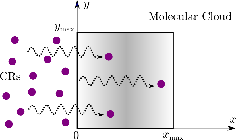
Figure 1: Schematic figure of CRs and a molecular cloud. CRs at $x<0$ intrude the molecular cloud at $0<x<x_{\rm max}$. The gas density of the cloud reaches the maximum at $x=x_{\rm max}/2$ as is shown by the gray shading.

At $t=0$, the cloud does not contain CRs. At $t>0$, CRs are injected at $x=0$. The CR spectrum at $x=0$ is represented as a broken power law:

$$f_{0}(p)=\left\{\begin{array}[]{ll}C\left(\frac{pc}{\rm GeV}\right)^{-\alpha}&(pc>1~{}{\rm GeV})\\ C\left(\frac{pc}{\rm GeV}\right)^{-2}&(pc<1~{}{\rm GeV})\end{array}\right.\>,\vspace{2mm}$$ (6)

where $\alpha~{}(>2)$ is a parameter. The normalization $C$ is given so that the total energy density of CRs at $pc>1$ GeV is $E_{\rm CR,tot}/V_{\rm SNR}$, where $E_{\rm CR,tot}$ is the total energy of CRs with $pc>1$ GeV accelerated at the SNR. The reason we adopt the broken power-law form is that if we assume a single power-law form with the index of $\alpha$, overabundant low-energy CRs ionize the cloud excessively and produce an overly bright 6.4 keV line for a given gamma-ray luminosity. This suggests that the low-energy CRs are injected somewhat differently from the higher-energy CRs. In the scenario proposed by Makino et al. (2019), the higher-energy CRs ($\gtrsim 1$ GeV) once escaped from the SNR when it was much younger and smaller. Then they diffuse in the interstellar space and enter the cloud. On the other hand, lower-energy CRs ($\lesssim 1$ GeV) are directly injected into the cloud from the SNR. This steepens the CR spectrum at $\gtrsim 1$ GeV because the CRs in the interstellar space are affected by energy-dependent diffusion in such a way that CRs with higher energies diffuse faster. Although the momentum-dependent escape process of the CRs must be considered in order to precisely derive the form of $f_{0}(p)$ (e.g. Li & Chen, 2010; Ohira et al., 2011), we here adopt the simplified model (equation (6)). It is to be noted that Phan et al. (2020) introduced a lower-energy limit in their CR spectrum instead of a broken power law.

We assume that the injection (equation (6)) is time-independent at $t>0$ for the sake of simplicity. We consider the intrusion of CRs on time-scales of $\leq 1\times 10^{4}$ yr, which is much smaller than the age of the SNR ($\sim 3\times 10^{4}$–$4\times 10^{4}$ yr). Thus, the injection may not change much during that period after the contact with the SNR.

2.3 Ionization Rates and Emissions

We consider the ionization of H₂, and the 6.4 keV line and gamma-ray emissions by CR protons. We ignore CR electrons because their contribution is subdominant for the 6.4 keV line and gamma-ray emissions for molecular clouds around SNRs (Nobukawa et al., 2018; Phan et al., 2020). The ionization of molecular clouds can also be explained by protons (Phan et al., 2020).

The ionization rate is given by

$$\zeta_{p}({\rm H}_{2}) = \int_{I({\rm H}_{2})}^{E_{\rm max}}n_{\rm CR}(E)v_{p}[1+\phi_{p}(E)]\sigma^{p}_{\rm ion}(E)dE$$ (7)

$$+\int_{0}^{E_{\rm max}}n_{\rm CR}(E)v_{p}\sigma_{\rm ec}(E)dE\>,$$

where $E$ is the kinetic energy of a particle corresponding to a momentum $p$, which means that $E=\sqrt{p^{2}c^{2}+m_{p}^{2}c^{4}}-m_{p}c^{2}$, where $m_{p}$ is the proton mass. For given $t$ and $x$, the CR density has a relation of $n_{\rm CR}(E)dE=4\pi p^{2}f(t,x,p)dp$. In equation (7), $I({\rm H}_{2})=15.603$ eV is the ionization potential of H₂, $E_{\rm max}~{}(=300~{}\rm TeV)$ is the maximum energy considered, and $\phi_{p}(E)$ is a correction factor accounting for the ionization of H₂ by secondary electrons (Padovani et al., 2009; Phan et al., 2018). For $\phi_{p}(E)$, we adopted the one derived by Krause et al. (2015). The quantities $\sigma^{p}_{\rm ion}$ and $\sigma_{\rm ec}$ are the proton ionization cross-section and the electron capture cross-section, respectively, and we use those obtained by Rudd et al. (1983) and Rudd et al. (1985).

The photon number intensity of the 6.4 keV neutral iron line is given by

$$I_{{\rm 6.4keV}}=\frac{1}{4\pi}\int dE\>\sigma_{\rm 6.4keV}(E)v_{p}\int d\ell\>n_{\rm H}(\ell)n_{{\rm CR}}(E,\ell)\>,$$ (8)

where $\sigma_{\rm 6.4keV}(E)$, $n_{\rm H}(\ell)$, and $\ell$ are the cross-section to produce the iron line at 6.4 keV, the number density of hydrogens in the molecular cloud, and the coordinate along the line of sight, respectively. Since the direction of $\ell$ is not necessarily perpendicular to that of $x$, the CR density $n_{{\rm CR}}$ includes the dependence on $\ell$ in equation (8). We derive gamma-ray spectra using the models by Kamae et al. (2006), Kelner et al. (2006), and Karlsson & Kamae (2008) based on $n_{\rm H}(\ell)$ and $n_{\rm CR}(E,\ell)$.

3 Results

We solve equation (1) using a standard implicit method. We adopt 200 unequally spaced meshes in the $x$-direction that cover the cloud. The mesh at $x\sim 0$ has a width of $\sim 3\times 10^{-4}$ pc, and the width of the mesh at $x\sim x_{\rm max}$ is $\sim 0.3$ pc. In this section, we show the results of our calculations for both the diffusive and free-streaming cases. We do not intend to precisely reproduce observations, but we rather focus on how results vary when parameters are changed. In particular, we study the profiles of $\zeta_{p}({\rm H}_{2})$, $I_{{\rm 6.4keV}}$, and gamma-ray surface brightness $I_{\gamma}$.

3.1 Diffusive Case

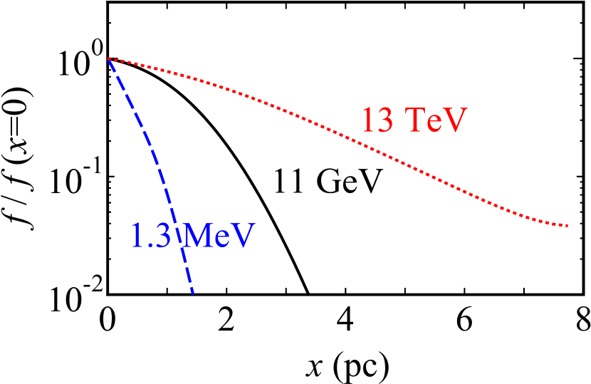
Figure 2: Distributions of CRs as functions of $x$ at $t=3000$ yr for the diffusive case: $E=1.3$ MeV (blue dashed line), $11$ GeV (black solid line), and 13 TeV (red dotted line)

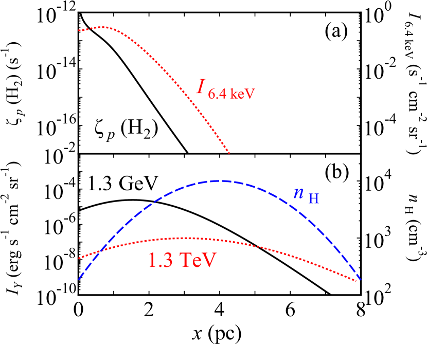
Figure 3: (a) Ionization rate ($\zeta_{p}({\rm H}_{2})$; black solid line) and surface brightness of the 6.4 keV line ($I_{{\rm 6.4keV}}$; red dotted line) as functions of $x$ at $t=3000$ yr for the diffusive case. (b) Gamma-ray surface brightness ($I_{\gamma}$) profiles at $E_{\gamma}=1.3$ GeV (black solid line) and $E_{\gamma}=1.3$ TeV (red dotted line) at $t=3000$ yr for the diffusive case. Hydrogen density profile (equation (5)) is also shown (blue dashed line).

Here, we assume that the line of sight ($\ell$) is parallel to the $y$-axis and it is perpendicular to the $x$-axis (Figure 1). In equation (2), we adopt a reduction factor of $\chi=0.01$, which is a typical value around SNRs (Fujita et al., 2009). The total energy of CRs with $pc>1$ GeV is $E_{\rm CR,tot}=1\times 10^{50}$ erg and the index is $\alpha=3.0$ (equation (6)), which are chosen so that the results are consistent with the observed gamma-ray luminosity of W 28. Figure 2 shows the distribution of CRs at $t=3000$ yr; CRs with higher energies can penetrate deeper inside the cloud because the diffusion coefficient is larger for them (equation (2)). On the other hand, lower-energy CRs ($\lesssim$ MeV) remain around $x\sim 0$ because they are affected by rapid cooling as well as the smaller diffusion coefficient. In Figure 3a, we present the profiles of the ionization rate $\zeta_{p}({\rm H}_{2})$ and the 6.4 keV line flux $I_{{\rm 6.4keV}}$. The former is a decreasing function of $x$ because lower-energy CRs, which ionize the gas, are concentrated around $x\sim 0$ (Figure 2). The 6.4 keV line emission is produced from slightly deeper in the cloud compared with the region of large $\zeta_{p}({\rm H}_{2})$ (Figure 3a). This is because while the ionization is mainly caused by CR protons with $E\sim 0.01$ MeV (Figure 1 in Padovani et al. 2009), the 6.4 keV line is attributed to those with $E\sim 10$ MeV (Figure 5 in Tatischeff et al. 2012). The latter CRs are less affected by cooling and diffuse more inside the cloud. The line intensity $I_{{\rm 6.4keV}}$ has a peak at $x\sim 0.7$ pc, because it reflects not only the CR density $n_{\rm CR}$ but also the hydrogen density $n_{\rm H}$ (equation (8) and Figure 3b). We note that the large values of $\zeta_{p}({\rm H}_{2})$ and $I_{{\rm 6.4keV}}$ at $x\sim 0$ should be regarded as the upper limits because it is unlikely that actual clouds are perfectly uniform along the line of sight.

Contrary to the large $\zeta_{p}({\rm H}_{2})$ and $I_{{\rm 6.4keV}}$ regions that are limited to $x\sim 0$, gamma-ray emissions are produced from almost the entire cloud especially for TeV gamma rays (Figure 3b). This is because CRs with higher energies ($\gtrsim$ TeV) can penetrate the cloud (Figure 2). Since the gamma-ray emissivity is proportional to $n_{\rm H}$, the gamma-ray profiles are subject to equation (5) that peaks at $x=4$ pc. The gamma-ray fluxes from the whole cloud are $F_{\gamma}=1.1\times 10^{-10}\rm\>erg\>cm^{-2}\>s^{-1}$ at $E_{\gamma}=1.3$ GeV, and $F_{\gamma}=1.1\times 10^{-12}\rm\>erg\>cm^{-2}\>s^{-1}$ at $E_{\gamma}=1.3$ TeV, which are close to the observed values for W 28 (Aharonian et al., 2008; Abdo et al., 2010b; Cui et al., 2018). It is to be noted that CRs with an energy of $E$ produce gamma rays with an energy of $E_{\gamma}\sim 0.1\>E$. In summary, the high $\zeta_{p}({\rm H}_{2})$ region should be observed close to the edge of the cloud, and $I_{{\rm 6.4keV}}$ has a similar distribution. On the other hand, the peak of the gamma-ray surface brightness is located deeper in the cloud. In particular, the profile of TeV gamma rays rather follows that of $n_{\rm H}$.

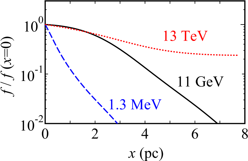
Figure 4: Same as Figure 2 but for $t=1\times 10^{4}$ yr.

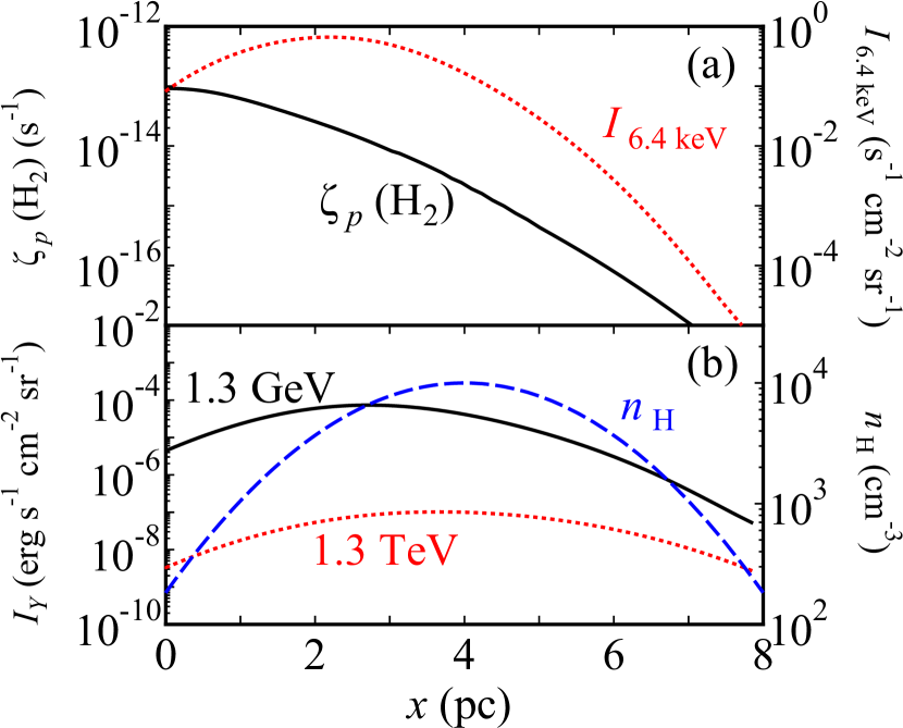
Figure 5: Same as Figure 3 but for $t=1\times 10^{4}$ yr.

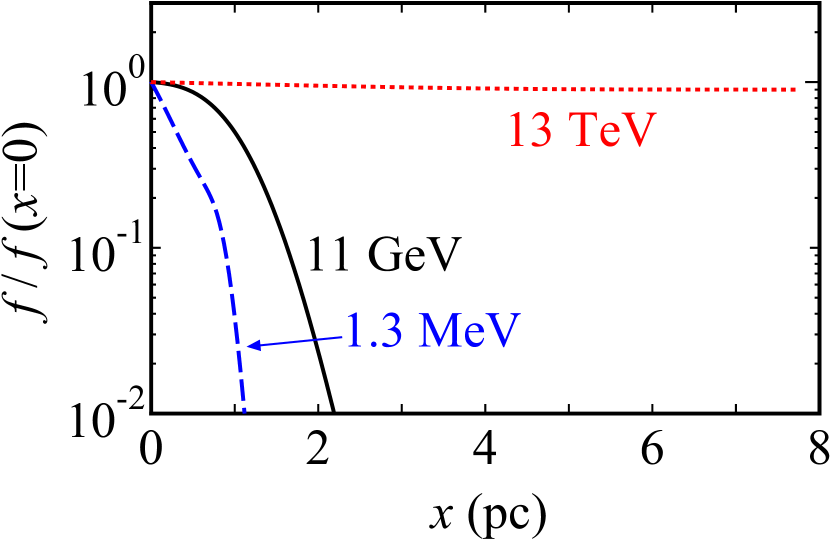
Figure 6: Same as Figure 2 ($t=3000$ yr) but in the case where the index of the diffusion coefficient is $\delta=1$.

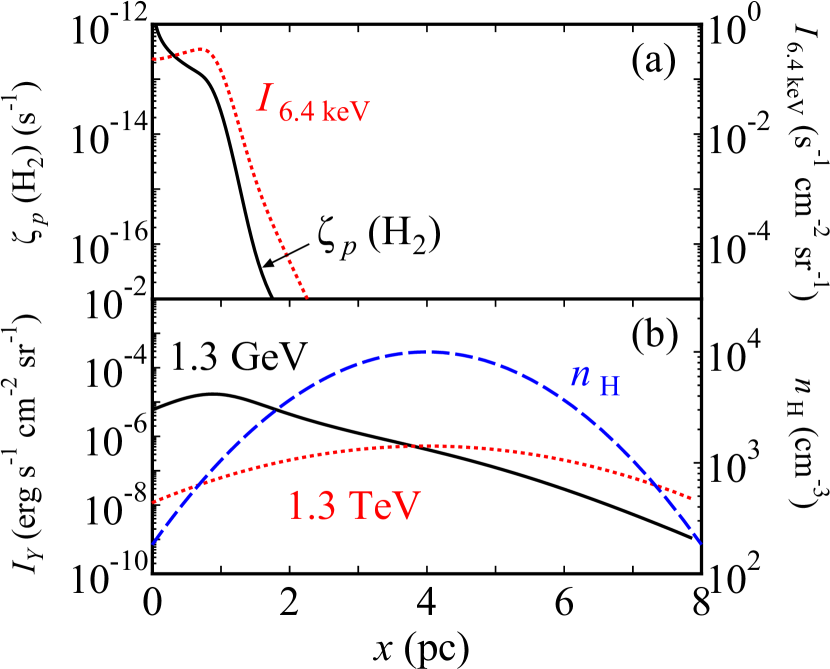
Figure 7: Same as Figure 3 ($t=3000$ yr) but in the case where the index of the diffusion coefficient is $\delta=1$.

If the line of sight is parallel to the $x$-axis (Figure 1), the flux of the observed 6.4 keV line is expected to be the volume-weighted summation along the $x$-axis because the 6.4 keV line is optically thin. In the case of Figure 3a, the flux along the $x$-axis is $\langle I_{{\rm 6.4keV}}\rangle=5.1\times 10^{-2}\rm\>photons\>s^{-1}\>cm^{-2}\>sr^{-1}$, which is consistent with the value observed for W 28 ($0.10^{+0.05}_{-0.05}\rm\>photons\>s^{-1}\>cm^{-2}\>sr^{-1}$; Nobukawa et al. 2018). If it is weighted by $n_{\rm H}$, the ionization rate averaged along the $x$-axis is $\langle\zeta_{p}({\rm H}_{2})\rangle=3.8\times 10^{-15}\rm\>s^{-1}$, which is roughly consistent with the ones for W 28 obtained by Vaupré et al. (2014) using DCO${}^{+}/$HCO⁺ abundance ratios. However, we note that if a molecular cloud is not uniform along the line of sight, the comparison of $\langle\zeta_{p}({\rm H}_{2})\rangle$ with the observed ionization rate is not trivial, because the observed rate also depends on the temperature structure of the cloud and the abundances of molecules (see also Padovani et al., 2009; Indriolo et al., 2010; Ceccarelli et al., 2011).

Figures 4 and 5 show the results for $t=1\times 10^{4}$ yr. Compared with Figures 2 and 3 ($t=3000$ yr), CRs enter further inside the cloud and gamma rays are produced there. While the peak of $\zeta_{p}({\rm H}_{2})$ is at $x=0$, that of TeV gamma rays is at $x\sim 4$ pc, where $n_{\rm H}$ reaches the maximum. The peaks of $I_{{\rm 6.4keV}}$ and GeV gamma rays are between them.

Figures 6 and 7 show the results when the index of the diffusion coefficient $D(p)$ is $\delta=1$ (equation (2)); other parameters are the same as those of the model of $\delta=1/3$. We consider this case because there are observations of CR transport in the heliosphere that suggest $D(p)\propto p$ at low energies (Bieber et al. 1994; Schlickeiser et al. 2010 and references therein). Compared with the case of $\delta=1/3$, $D(p)$ is much smaller (larger) at $pc\ll 10$ GeV ($pc\gg 10$ GeV). Thus, the lower-energy CRs cannot penetrate deep inside the cloud, while the higher-energy CRs can prevail in the cloud (Figure 6). This explains why the tendencies shown in Figure 3 are strengthened in Figure 7 in which large $\zeta_{p}({\rm H}_{2})$ and $I_{{\rm 6.4keV}}$ regions are more confined at $x\sim 0$, while TeV gamma-ray emissions come from the entire cloud.

3.2 Free-streaming Case

Figures 8 and 9 show the results for the free-streaming case. While most parameters are the same as those for the diffusive case, we need to reduce the total CR energy to $E_{\rm CR,tot}=5\times 10^{48}$ erg (or increase $V_{\rm SNR}$ by 20 times) and adopt $\alpha=2.8$ (equation (6)) to reproduce the observed total gamma-ray fluxes. This is because in this model both GeV and TeV CRs freely penetrate into the cloud without cooling (Figure 8) and effectively produce gamma rays through interaction with high-density gas at $x\sim 4$ pc (Figure 9b). The total gamma-ray fluxes are $F_{\gamma}=1.3\times 10^{-10}\rm\>erg\>cm^{-2}\>s^{-1}$ at $E_{\gamma}=1.3$ GeV, and $F_{\gamma}=1.0\times 10^{-12}\rm\>erg\>cm^{-2}\>s^{-1}$ at $E_{\gamma}=1.3$ TeV. Since GeV-TeV CRs are uniformly distributed in the cloud (Figure 8), the gamma-ray profiles simply reflect the gas density $n_{\rm H}$ (Figure 9b).

Contrary to the high-energy CRs, lower-energy CRs ($E\lesssim 10$ MeV) cool before they traverse the cloud and reach $x=x_{\rm max}$. Thus, their number density decreases as $x$ increases (blue dashed line in Figure 8) and the ionization rate $\zeta_{p}({\rm H}_{2})$ simply reflects that profile when the line of sight ($\ell$) is parallel to the $y$-axis (Figure 9a). On the other hand, the energy of the CRs that most contribute to the 6.4 keV line is $E\sim 10$ MeV (Figure 5 in Tatischeff et al. 2012). These CRs are marginally immune to the rapid cooling and are distributed almost uniformly in the cloud. Thus, the profile of $I_{{\rm 6.4keV}}$ follows that of $n_{\rm H}$ (equation (8)), which is the same as the gamma-ray profiles (Figure 9). This presents a contrast to the the diffusive case (section 3.1). When the line of sight is parallel to the $x$-axis, the mass-averaged ionization rate is $\langle\zeta_{p}({\rm H}_{2})\rangle=7.5\times 10^{-15}\rm\>s^{-1}$, and the 6.4 keV line flux is $\langle I_{{\rm 6.4keV}}\rangle=0.22\rm\;photons\;s^{-1}\>cm^{-2}\>sr^{-1}$. The results for $t=1\times 10^{4}$ yr are almost the same as those for $t=3000$ yr.

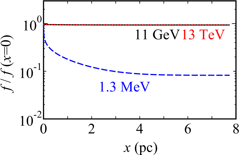
Figure 8: Same as Figure 2 ($t=3000$ yr) but for the free-streaming case.

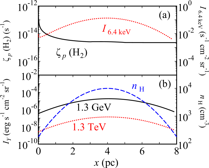
Figure 9: Same as Figure 3 ($t=3000$ yr) but for the free-streaming case.

4 Discussion

We have obtained the profiles of the ionization rate $\zeta_{p}({\rm H}_{2})$, the 6.4 keV line intensity $I_{{\rm 6.4keV}}$, and the gamma-ray surface brightness $I_{\gamma}$ for a molecular cloud exposed to CRs. We found that for both the diffusive and free-streaming CR propagation cases, large $\zeta_{p}({\rm H}_{2})$ regions are limited to the edge of the cloud due to the rapid cooling of low-energy CRs that are responsible for the ionization. In both cases, TeV gamma rays come from the dense core of the cloud because high-energy CRs associated with the radiation can penetrate deep into the cloud. In the diffusive case, $I_{{\rm 6.4keV}}$ has a profile similar to that of $\zeta_{p}({\rm H}_{2})$, although the peak is located slightly inside the cloud. The GeV gamma-ray profile has a shape that is intermediate between $I_{{\rm 6.4keV}}$ and TeV gamma-ray profiles. In the free-streaming case, both $I_{{\rm 6.4keV}}$ and GeV gamma rays have profiles similar to that of TeV gamma rays. This is because CRs with $E\gtrsim 10$ MeV are uniformly distributed in the cloud with being less affected by cooling and their profiles reflect the gas density profile of the cloud.

While many SNRs have been observed in gamma rays, the number of SNRs for which ionization rates, 6.4 keV line and gamma-ray fluxes are all obtained is limited. The exceptions are W 28, IC 443, and W 51C. Since our model is rather simple, we here qualitatively compare our predictions with the observations. For W 28, ionization rates have been obtained through DCO⁺/HCO⁺ abundance ratios (Vaupré et al., 2014) and 6.4 keV line fluxes have been measured with Suzaku (Nobukawa et al., 2018; Okon et al., 2018). Nobukawa et al. (2018) indicated that the 6.4 keV line emitting region is shifted from the center of the northeastern molecular cloud and the TeV gamma-ray emitting region (Aharonian et al., 2008), while Okon et al. (2018) detected the 6.4 keV line in the gamma-ray emitting region. The former and the latter favor the diffusive case (section 3.1) and the free-streaming case (section 3.2), respectively. Nobukawa et al. (2018) analyzed X-ray spectra for regions selected based on an X-ray image in a narrow band including the 6.4 keV line, while Okon et al. (2018) performed spectral analysis for a few specific regions irrespective of the narrow band image. The apparent discrepancy of the position of the line emitting region may indicate some uncertainty in current X-ray observations. High ionization rates are discovered at the tip of the cloud (Figure 1 in Phan et al., 2020). Unfortunately, ionization rates are studied only for limited areas and they are not obtained for the regions where the 6.4 keV line is detected by Nobukawa et al. (2018). If the diffusive case is correct, the ionization rates should be high there.

For W 28, we examine the possibility that the 6.4 keV line is created by X-rays rather than CRs. Figure 5 in Okon et al. (2018) shows that the X-ray radiation at the energy of $E_{X}>7$ keV, which is responsible for the 6.4 keV line, is dominated by background emissions. The intensity of the 6.4 keV line created by the emissions is estimated as

$$I_{\rm 6.4keV}=\epsilon\int_{E_{\rm Ked}}^{\infty}[1-\exp{(-N_{\rm H}Z_{\rm Fe}\sigma_{\rm Fe}(E_{X}))}]I_{b}(E_{X})dE_{X}\>,$$ (9)

where $\epsilon=0.34$ (Bambynek et al., 1972) is the iron fluorescence yield, $E_{\rm Ked}=7.1$ keV is the energy of the iron K-edge, $N_{\rm H}$ is the hydrogen column density of the molecular cloud, $Z_{\rm Fe}$ is the iron abundance, $\sigma_{\rm Fe}(E_{X})$ is the cross-section of the iron photoionization, and $I_{b}(E_{X})$ is the flux of the X-ray background. Here, we adopt $\sigma_{\rm Fe}(E_{X})\approx 6.0\times 10^{-18}E_{X}^{-2.6}\rm\>cm^{2}$ (Henke et al., 1982). The background flux is estimated from that in the reference region studied by Nobukawa et al. (2018) and it is represented by $I_{b}(E_{X})\approx 1.2\times 10^{-5}\>E^{-2.3}\rm\>photons\>keV^{-1}\>cm^{-2}\>s^{-1}\>arcmin^{-2}$. If we assume that $N_{H}=3\times 10^{22}\rm\>cm^{-2}$ and $Z_{\rm Fe}=3\times 10^{-5}$ (solar abundance; Lodders 2003), we obtain $I_{\rm 6.4keV}=3.0\times 10^{-9}\rm\>photons\>cm^{-2}\>s^{-1}\>arcmin^{-2}$, which is 1 order of magnitude smaller than those observationally obtained by Nobukawa et al. (2018) and Okon et al. (2018). If the value of $N_{\rm H}$ is smaller around the cloud edge (see equation (5)), $I_{\rm 6.4keV}$ becomes even smaller. Thus, we conclude that the contribution of X-rays to the observed 6.4 keV line intensity is minor.

For IC 443, one of the regions that are emitting the 6.4 keV line (Reg 2 in Figure 1 of Nobukawa et al., 2019) is close to the centroids of GeV–TeV gamma-ray sources (Albert et al., 2007; Acciari et al., 2009; Abdo et al., 2010c), which favors the free-streaming case (Figure 9). Another region from which the 6.4 keV line is detected (Reg 1 in Figure 1 of Nobukawa et al., 2019) is shifted from the gamma-ray centroids. Ionization rates have been measured for several points around the SNR (Indriolo et al., 2010). Two of the points (ALS 8828 and HD 254577) show high ionization rates. We found that ALS 8828 is very close to Reg 1. Thus, Reg 1 may be described by the diffusive case (Figure 3). HD 254577 is not associated with gamma rays. There is no report about the 6.4 keV line at HD 254577 and there is no measurement of ionization rates in Reg 2.

For W 51C, it has been indicated that a high ionization point coincides with a gamma-ray source (Ceccarelli et al. 2011; see also Abdo et al. 2009; Aleksić et al. 2012). Suzaku X-ray observations also suggest that the 6.4 keV line emission comes from the same region (Shimaguchi et al. in preparation). However, the relatively small angular size of the SNR does not allow us to discuss their relative positions in detail.

We note that in the above discussions we implicitly assumed that the line of sight is perpendicular to the direction of CR diffusion or stream ($x$-axis in Figure 1). If the line of sight is parallel to the $x$-axis, high ionization rates could be measured where both the 6.4 keV line and gamma-ray emissions are detected, regardless of the diffusive and free-streaming cases. Reg 2 in IC 443 could be such an example because it is apparently located well inside the the SNR (Nobukawa et al., 2019) and three-dimensionally it could be behind or in front of the SNR. Statistical studies with more samples may be required to investigate the three-dimensional effect. In summary, so far there is no strong evidence that either of the diffusive or free-streaming intrusion is dominant considering observational uncertainties.

In the near future, the advent of XRISM and Athena will make it possible to measure the spectral profile of the 6.4 keV line in more detail. Recently, Okon et al. (2020) indicated that the iron line substructures generated by the multiple ionization process can be direct evidence that the line is produced by CRs rather than X-rays. Those satellites will be able to resolve the substructures. For ionization rates, it is desirable to make intensive observations that cover wide fields around SNRs using radio telescopes such as Nobeyama 45 m and ALMA.

5 Conclusion

Using an 1D model, we have studied the spatial correlation among the ionization rates of dense gas, the 6.4 keV line intensity, and the gamma-ray emissions from a molecular cloud illuminated by CRs accelerated at an adjacent SNR. We found that the profiles of the three observables depend on how CRs intrude the cloud and on the internal structure of the cloud. If the CRs diffusively enter the cloud and the diffusion coefficient is relatively small, the 6.4 keV line should be detected in the cloud outskirts where ionization rates are high. This is because the 6.4 keV line and the ionization are attributed to CRs with energies of $\lesssim 10$ MeV. Those CRs cool before they penetrate the cloud. On the other hand, if CRs freely move in the cloud, the 6.4 keV line profiles should be similar to gamma-ray profiles. The energies of the CRs associated with the 6.4 keV line ($\sim 10$ MeV) are higher than those associated with the ionization ($\sim 0.01$ MeV). Thus, the former can traverse the cloud before cooling in the same way as gamma-ray emitting CRs with higher energies. Both the 6.4 keV line flux and gamma-ray profiles follow the gas profiles of the cloud. We compared the results with observations and argued whether the diffusive or the free-streaming intrusion is realized. However, we could not draw an unambiguous conclusion mostly because of observational uncertainties.

References

- Abdo et al. (2009) Abdo, A. A., Ackermann, M., Ajello, M., et al. 2009, ApJ, 706, L1, doi: 10.1088/0004-637X/706/1/L1
- Abdo et al. (2010a) —. 2010a, Science, 327, 1103, doi: 10.1126/science.1182787
- Abdo et al. (2010b) —. 2010b, ApJ, 718, 348, doi: 10.1088/0004-637X/718/1/348
- Abdo et al. (2010c) —. 2010c, ApJ, 712, 459, doi: 10.1088/0004-637X/712/1/459
- Acciari et al. (2009) Acciari, V. A., Aliu, E., Arlen, T., et al. 2009, ApJ, 698, L133, doi: 10.1088/0004-637X/698/2/L133
- Ackermann et al. (2013) Ackermann, M., Ajello, M., Allafort, A., et al. 2013, Science, 339, 807, doi: 10.1126/science.1231160
- Aharonian et al. (2008) Aharonian, F., Akhperjanian, A. G., Bazer-Bachi, A. R., et al. 2008, A&A, 481, 401, doi: 10.1051/0004-6361:20077765
- Albert et al. (2007) Albert, J., Aliu, E., Anderhub, H., et al. 2007, ApJ, 664, L87, doi: 10.1086/520957
- Aleksić et al. (2012) Aleksić, J., Alvarez, E. A., Antonelli, L. A., et al. 2012, A&A, 541, A13, doi: 10.1051/0004-6361/201218846
- Bamba et al. (2018) Bamba, A., Ohira, Y., Yamazaki, R., et al. 2018, ApJ, 854, 71, doi: 10.3847/1538-4357/aaa5a0
- Bambynek et al. (1972) Bambynek, W., Crasemann, B., Fink, R. W., et al. 1972, Reviews of Modern Physics, 44, 716, doi: 10.1103/RevModPhys.44.716
- Bieber et al. (1994) Bieber, J. W., Matthaeus, W. H., Smith, C. W., et al. 1994, ApJ, 420, 294, doi: 10.1086/173559
- Ceccarelli et al. (2011) Ceccarelli, C., Hily-Blant, P., Montmerle, T., et al. 2011, ApJ, 740, L4, doi: 10.1088/2041-8205/740/1/L4
- Cui et al. (2018) Cui, Y., Yeung, P. K. H., Tam, P. H. T., & Pühlhofer, G. 2018, ApJ, 860, 69, doi: 10.3847/1538-4357/aac37b
- Dogiel et al. (2018) Dogiel, V. A., Chernyshov, D. O., Ivlev, A. V., et al. 2018, ApJ, 868, 114, doi: 10.3847/1538-4357/aae827
- Fujita et al. (2010) Fujita, Y., Ohira, Y., & Takahara, F. 2010, ApJ, 712, L153, doi: 10.1088/2041-8205/712/2/L153
- Fujita et al. (2009) Fujita, Y., Ohira, Y., Tanaka, S. J., & Takahara, F. 2009, ApJ, 707, L179, doi: 10.1088/0004-637X/707/2/L179
- Fujita et al. (2011) Fujita, Y., Takahara, F., Ohira, Y., & Iwasaki, K. 2011, MNRAS, 415, 3434, doi: 10.1111/j.1365-2966.2011.18980.x
- Gabici et al. (2009) Gabici, S., Aharonian, F. A., & Casanova, S. 2009, MNRAS, 396, 1629, doi: 10.1111/j.1365-2966.2009.14832.x
- Henke et al. (1982) Henke, B. L., Lee, P., Tanaka, T. J., Shimabukuro, R. L., & Fujikawa, B. K. 1982, Atomic Data and Nuclear Data Tables, 27, 1, doi: 10.1016/0092-640X(82)90002-X
- Indriolo et al. (2010) Indriolo, N., Blake, G. A., Goto, M., et al. 2010, ApJ, 724, 1357, doi: 10.1088/0004-637X/724/2/1357
- Inoue (2019) Inoue, T. 2019, ApJ, 872, 46, doi: 10.3847/1538-4357/aafb70
- Ivlev et al. (2018) Ivlev, A. V., Dogiel, V. A., Chernyshov, D. O., et al. 2018, ApJ, 855, 23, doi: 10.3847/1538-4357/aaadb9
- Kamae et al. (2006) Kamae, T., Karlsson, N., Mizuno, T., Abe, T., & Koi, T. 2006, ApJ, 647, 692, doi: 10.1086/505189
- Karlsson & Kamae (2008) Karlsson, N., & Kamae, T. 2008, ApJ, 674, 278, doi: 10.1086/524353
- Kelner et al. (2006) Kelner, S. R., Aharonian, F. A., & Bugayov, V. V. 2006, Phys. Rev. D, 74, 034018, doi: 10.1103/PhysRevD.74.034018
- Krause et al. (2015) Krause, J., Morlino, G., & Gabici, S. 2015, in International Cosmic Ray Conference, Vol. 34, 34th International Cosmic Ray Conference (ICRC2015), 518
- Kulsrud & Pearce (1969) Kulsrud, R., & Pearce, W. P. 1969, ApJ, 156, 445, doi: 10.1086/149981
- Li & Chen (2010) Li, H., & Chen, Y. 2010, MNRAS, 409, L35, doi: 10.1111/j.1745-3933.2010.00944.x
- Lodders (2003) Lodders, K. 2003, ApJ, 591, 1220, doi: 10.1086/375492
- Makino et al. (2019) Makino, K., Fujita, Y., Nobukawa, K. K., Matsumoto, H., & Ohira, Y. 2019, PASJ, 71, 78, doi: 10.1093/pasj/psz058
- Mannheim & Schlickeiser (1994) Mannheim, K., & Schlickeiser, R. 1994, A&A, 286, 983. https://arxiv.org/abs/astro-ph/9402042
- Morlino & Gabici (2015) Morlino, G., & Gabici, S. 2015, MNRAS, 451, L100, doi: 10.1093/mnrasl/slv074
- Nobukawa et al. (2019) Nobukawa, K. K., Hirayama, A., Shimaguchi, A., et al. 2019, PASJ, 71, 115, doi: 10.1093/pasj/psz099
- Nobukawa et al. (2018) Nobukawa, K. K., Nobukawa, M., Koyama, K., et al. 2018, ApJ, 854, 87, doi: 10.3847/1538-4357/aaa8dc
- Ohira et al. (2011) Ohira, Y., Murase, K., & Yamazaki, R. 2011, MNRAS, 410, 1577, doi: 10.1111/j.1365-2966.2010.17539.x
- Okon et al. (2020) Okon, H., Imai, M., Tanaka, T., Uchida, H., & Tsuru, T. G. 2020, PASJ, 72, L7, doi: 10.1093/pasj/psaa055
- Okon et al. (2018) Okon, H., Uchida, H., Tanaka, T., Matsumura, H., & Tsuru, T. G. 2018, PASJ, 70, 35, doi: 10.1093/pasj/psy022
- Padovani et al. (2009) Padovani, M., Galli, D., & Glassgold, A. E. 2009, A&A, 501, 619, doi: 10.1051/0004-6361/200911794
- Phan et al. (2020) Phan, V. H. M., Gabici, S., Morlino, G., et al. 2020, A&A, 635, A40, doi: 10.1051/0004-6361/201936927
- Phan et al. (2018) Phan, V. H. M., Morlino, G., & Gabici, S. 2018, MNRAS, 480, 5167, doi: 10.1093/mnras/sty2235
- Ptuskin et al. (2008) Ptuskin, V. S., Zirakashvili, V. N., & Plesser, A. A. 2008, Advances in Space Research, 42, 486, doi: 10.1016/j.asr.2007.12.007
- Rho & Borkowski (2002) Rho, J., & Borkowski, K. J. 2002, ApJ, 575, 201, doi: 10.1086/341192
- Rudd et al. (1983) Rudd, M. E., Goffe, T. V., Dubois, R. D., Toburen, L. H., & Ratcliffe, C. A. 1983, Phys. Rev. A, 28, 3244, doi: 10.1103/PhysRevA.28.3244
- Rudd et al. (1985) Rudd, M. E., Kim, Y. K., Madison, D. H., & Gallagher, J. W. 1985, Reviews of Modern Physics, 57, 965, doi: 10.1103/RevModPhys.57.965
- Saji et al. (2018) Saji, S., Matsumoto, H., Nobukawa, M., et al. 2018, PASJ, 70, 23, doi: 10.1093/pasj/psx158
- Sato et al. (2016) Sato, T., Koyama, K., Lee, S.-H., & Takahashi, T. 2016, PASJ, 68, S8, doi: 10.1093/pasj/psv131
- Sato et al. (2014) Sato, T., Koyama, K., Takahashi, T., Odaka, H., & Nakashima, S. 2014, PASJ, 66, 124, doi: 10.1093/pasj/psu120
- Schlickeiser et al. (2010) Schlickeiser, R., Lazar, M., & Vukcevic, M. 2010, ApJ, 719, 1497, doi: 10.1088/0004-637X/719/2/1497
- Silsbee & Ivlev (2019) Silsbee, K., & Ivlev, A. V. 2019, ApJ, 879, 14, doi: 10.3847/1538-4357/ab22b4
- Tatischeff et al. (2012) Tatischeff, V., Decourchelle, A., & Maurin, G. 2012, A&A, 546, A88, doi: 10.1051/0004-6361/201219016
- Tavani et al. (2010) Tavani, M., Giuliani, A., Chen, A. W., et al. 2010, ApJ, 710, L151, doi: 10.1088/2041-8205/710/2/L151
- Vaupré et al. (2014) Vaupré, S., Hily-Blant, P., Ceccarelli, C., et al. 2014, A&A, 568, A50, doi: 10.1051/0004-6361/201424036
- Velázquez et al. (2002) Velázquez, P. F., Dubner, G. M., Goss, W. M., & Green, A. J. 2002, AJ, 124, 2145, doi: 10.1086/342936
- Wentzel (1969) Wentzel, D. G. 1969, ApJ, 156, 303, doi: 10.1086/149965
- Zweibel & Shull (1982) Zweibel, E. G., & Shull, J. M. 1982, ApJ, 259, 859, doi: 10.1086/160220