Uncertainties in the Galactic Dark Matter Distribution: an Update

Abstract

We present here a quantitative estimate of the impact of uncertainties of astrophysical nature on the determination of the dark matter distribution within our Galaxy, the Milky Way. Based on an update of a previous analysis, this work is motivated by recent new determinations of astrophysical quantities of relevance –such as the Galactic parameters (R₀,V₀)– from the GRAVITY collaboration and the GAIA satellite, respectively. We find that even with these state–of–the–art determination and a range of uncertainties –both statistical and systematic– much narrowed with respect to previous literature, the uncertainties on the dark matter distribution and their impact on searches of physics beyond the standard model stays sizable.

1 Introduction

The determination of the gravitational structure of our host Galaxy, the Milky Way (MW), is a very interesting endeavor by itself, and at the same time it has implications that reverberate from Cosmology to Particle Physics. The gravitational potential of the MW can not be explained by the presence of stars and gas alone, beyond the innermost $\sim$ 5 kpc, [1]. This is generally imputed to the presence of a component of unknown nature dubbed Dark Matter (DM). On the one hand, this component of matter cannot be accommodated within the Standard Model of Particle Physics. This has motivated direct and indirect particle searches, together with collider experiments, that aim to understand its nature. Synergies between these efforts have constrained the parameter space of several extensions of the Standard Model. However, these attempts are hampered since the interpretation of data from direct and indirect searches depends on the distribution of DM in the Galaxy. On the other hand, the distribution of DM in galaxies is a prediction of the $\Lambda$CDM model, thus it provides an important test of consistency of the cosmological framework.

From the above, it proceeds that the distribution of the DM within our Galaxy is of relevance, beside its intrinsic value “per se”, as an ancillary quantity for other fields. Determined through techniques that rely on astrophysical observations [2, 3, 4, 5, 6, 7, 8, 9, 10, 11, 12, 13, 14, 15], the DM distribution is unavoidably affected by the uncertainties that plague such observations. Such uncertainties do propagate into other quantities that rely on the use of the DM distribution, and hence the original ignorance on astrophysical quantities propagate to quantities of seemingly unrelated nature, such as the so-called DM $J$-factor which regulates the amount of DM annihilation signal and thus the expected yield of e.g. $\gamma$-ray photons, neutrinos or antiprotons, which would reveal the presence of DM itself, or the local DM density $\rho_{0}$ which, instead, dictates the expected number of events in underground direct detection experiments [16].

The principles of the above are very well known, yet a specific quantitative approach, systematically estimating the effect of all the observables into play, is not thoroughly adopted. In a previous work [6] we had proposed a first quantitative estimate of the impact of astrophysical uncertainties on specific scenarios for the DM nature. Later, we had proposed a systematic approach to the astrophysical quantities in play in the empirical determination of the DM distribution [16] (hereafter Paper I). In Paper I, we also presented a likelihood function that can be used in the particle interpretation of data coming from direct and indirect searches in order to self-consistently include astrophysical uncertainties that affect our determination of the DM distribution [17, 18, 19, 20, 21, 22, 23, 24, 25].

In this new paper, we present an approach very similar to that of Paper I, slightly modified from the technical point of view, and including the recent most determinations of some of the astrophysical quantities that have a bigger impact in the determination of the DM distribution, namely the Sun’s distance to the Galactic center, $R_{0}$, and its circular velocity $V_{0}$. We anticipate that despite uncertainties on these quantities are narrowed, the remaining uncertainties on the DM distribution are sizable, thus still affecting searches for its nature.

This paper is structured as follows: in section 2 we describe the new methodology; in section 3 we present the new observations we adopt for this determination; in section 4 we present our results, also comparing the state–of–the–art and the improvement of knowledge with respect to previous determinations. We present our conclusions in section 5, while in Appendix A and B we discuss the case of alternative DM profiles, and in Appendix C we provide the results of a Bayesian analysis and compare them with the frequentist analysis.

2 Methodology

We closely follow the data-driven analysis presented in Paper I in order to quantify astrophysical uncertainties on our determination of the DM distribution in the MW. In particular, constraints on the distribution of DM are obtained with the well-known rotation curve (RC) method, by comparing the observed RC of the MW with predicted velocities expected to be caused by the baryonic and DM components of the Galaxy.

We adopt the data from the galkin compilation [1, 26] for the observed RC. Observed velocities depend on the Sun’s galactocentric distance $R_{0}$, its circular velocity $V_{0}$ and its peculiar motion $(U,V,W)_{\odot}$. The Sun’s peculiar motion in the tangential direction $V_{\odot}$, $R_{0}$ and $V_{0}$ are related to the Sun’s total angular velocity, $\Omega_{\rm 0,tot}$, by

$$\Omega_{\rm 0,tot}=\frac{V_{\rm 0,tot}}{R_{0}}=\frac{V_{0}+V_{\odot}}{R_{0}}.$$ (1)

In Paper I [16], we fixed $\Omega_{\rm 0,tot}$, whose value is known with a small uncertainty, and $V_{\odot}$, and we varied $R_{0}$ in the range 7.5-8.5 kpc. Each time $R_{0}$ is specified, $V_{0}$ was derived following the above equation. The generous range of variation for $R_{0}$ was in part compensating for having kept fixed $V_{\odot}$, thus neglecting its uncertainty. In this work we rather fix $\Omega_{\rm 0,tot}$ and $R_{0}$, which has been recently precisely measured (see below), and we vary $V_{0}$ within measured uncertainties. Each time $V_{0}$ is specified, $V_{\odot}$ is obtained by means of equation (1). That is, the quantities $V_{0}$ and $V_{\odot}$ self-consistently satisfy constraints on the Solar total velocity in the tangential direction, which is estimated with high precision [27].

We assume the DM is a smooth, spherically-symmetric component whose distribution is described by a generalized Navarro-Frenk-White (gNFW) profile [28, 29] (in appendices A and B we show the results for the Burkert [30] and Einasto [31] DM density profiles, respectively). For the baryonic matter, we adopt a set of several baryonic morphologies $\mathcal{M}_{i}$ – motivated by observations – that bracket the systematic uncertainty on the distribution of the baryonic mass in our Galaxy [1]. A complete description of the the baryonic morphology catalog can be found in [1, 16] and references therein. We also account for the uncertainty on the total baryonic mass by normalizing the stellar disk profile to the stellar surface density at the Sun’s position $\Sigma_{*}$ and by normalizing the bulge mass using the microlensing optical depth towards the galactic center $\langle\tau\rangle$.

Our analysis has, thus, the following free parameters: $V_{0}$, $\Theta$, $\mathcal{M}_{i}$, $\langle\tau\rangle$ and $\Sigma_{*}$; where $\Theta=(R_{s},\rho_{0},\gamma)$ correspond to the parameters of the DM density profile, i.e. the profile scale radius, the local DM density and the profile inner slope, respectively. We scan a discrete grid composed of 50 values for $\rho_{0}$ linearly spaced in the range [0, 1] $\rm GeV/cm^{3}$, 50 values for $R_{s}$ logarithmically spaced in the range [5, 100] kpc, 15 values of $\gamma$ linearly spaced in the range [0, 1.5], 10 values of $V_{0}$ linearly spaced in the range [218, 240] km/s, and 30 morphologies $\mathcal{M}_{i}$. For $\langle\tau\rangle$ and $\Sigma_{*}$ we use 10 values each, linearly spaces in the range [-2$\sigma$, +2$\sigma$]. At each point of this seven-dimensional grid, observed and predicted rotation velocities are compared by means of a $\chi^{2}$ statistics given by

$$\begin{split}\chi^{2}_{\rm RC}(V_{0},\Theta,\mathcal{M}_{i},\langle\tau\rangle,\Sigma_{*})=&\sum_{j}\frac{\left(\bar{w}_{j}(\Theta,\mathcal{M}_{i},\langle\tau\rangle,\Sigma_{*})-\bar{w}^{obs}_{j}(V_{0})\right)^{2}}{\sigma_{\bar{w}_{j}}^{2}}\\ &+\frac{\left(\langle\tau\rangle-\langle\tau\rangle^{obs}\right)^{2}}{\sigma_{\langle\tau\rangle}^{2}}+\frac{\left(\Sigma_{*}-\Sigma_{*}^{obs}\right)^{2}}{\sigma_{\Sigma_{*}}^{2}},\end{split}$$ (2)

where $\bar{w}^{obs}_{j}$ is the measured angular velocity, with its corresponding uncertainty $\sigma_{\bar{w}_{j}}$, for a given radial RC bin $j$. For details on how the binned quantities $\bar{w}^{obs}_{j}$ and $\sigma_{\bar{w}_{j}}$ are derived from the galkin compilation of measurements we refer the reader to Paper I. We also notice that for each different values of $V_{0}$ on the grid the experimental angular velocities also change accordingly. We self-consistently take this effect into account. Again, this is discussed in detail in Paper I. We adopt the values of the microlensing optical depth measurement provided in [32], i.e. $\langle\tau\rangle^{obs}=2.17^{+0.47}_{-0.38}\times 10^{-6}$, as well as the stellar surface density at the Sun’s position provided by [3], namely $\Sigma_{*}^{obs}=(38\pm 4){\rm M_{\odot}/pc^{2}}$. For simplicity, we symmetrize the error in the microlensing optical depth and adopt a standard deviation of $\sigma_{\langle\tau\rangle}=0.47$.

We employ a frequentist formalism and derive profile likelihoods. For a thorough description of the statistical framework, we refer the interested reader to section 3 in Paper I. Nonetheless, for completeness, we also present bayesian results, which do not rely on a grid but make use of Monte Carlo scan techniques. The results of the Bayesian analysis are reported in appendix C.

3 New observations

In this work we adopt the following new estimates of the relevant astrophysical quantities $(R_{0},V_{0})$:

• the Sun’s galactocentric distance estimation obtained by the GRAVITY collaboration by measuring the Keplerian orbit of the S2 star in the innermost parsecs of the Galaxy [33]:

  $$R_{0}=8.178\pm 0.013{\rm(stat)}\pm 0.022{\rm(syst)}.$$ (3)

• The Sun’s circular velocity determined by means of a Jeans analysis that combines Gaia [34], WISE [35] and 2MASS [36] photometry with spectral data from APOGEE [37] for $\sim 23000$ red-giant stars with galactocentric distances between 5 and 25 kpc [38]:

  $$V_{0}=229.0\pm 0.2\,{\rm km/s},$$ (4)

  with a systematic uncertainty in the range $2-5$%.

We fix $R_{0}$ to the GRAVITY estimate and we vary $V_{0}$ within measured uncertainties. We adopt as fiducial the $V_{0}$ range $[218,240]\,{\rm km/s}$, chosen to encompass the conservative 5% systematic uncertainty quoted in [38], and incidentally coinciding with the range of values found in the literature (e.g. [40, 41, 42, 43, 44, 45]).

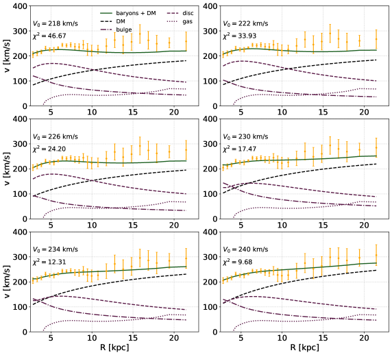
Figure 1: Observed Rotation Curve and best-fit contributions of the bulge, disc, gas, DM, individually as well as summed together, for different values of $V_{0}$. The slope of the DM profile (gNFW) has been fixed to $\gamma=1$ for these plots (see text for more details).

As in Paper I, the Solar total angular velocity is fixed to the precise result $\Omega_{\rm 0,tot}=30.24\pm 0.12\,{\rm km/s/kpc}$, which is obtained by measuring the proper motion of Sgr A^∗ [52]. The Sun’s peculiar motion in the radial and vertical directions are fixed to $U_{\odot}=11.10\,\rm km/s$ and $W_{\odot}=7.25\,\rm km/s$ [43], respectively. These two quantities are measured with $\sim 10\%$ precision see e.g. [42] and references therein. By varying them within measured uncertainties, our results remain unaffected. It is to be noticed that whether $U_{\odot}$ and $W_{\odot}$ are measured with the indicated precision, large scatter surrounds the estimates of $V_{\odot}$. In fact, the range of $V_{\odot}$ values adopted in this work, which spans $22\text{\,}\mathrm{k}\mathrm{m}\mathrm{/}\mathrm{s}$, encompasses global and local estimates found in the literature [46, 47, 48, 49, 50, 41, 51]. Sizeable uncertainties on this parameter might be explained by streaming motion induced by local substructures or/and spiral arms [42].

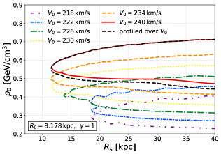
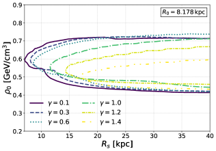
Figure 2: Top panel: 2$\sigma$ contours in the $(R_{s},\rho_{0})$ plane for fixed $\gamma=1$ and $R_{0}={8.178}\,{\rm kpc}$, and for various values of $V_{0}$, and profiled over $\mathcal{M}_{i}$, $\langle\tau\rangle$ and $\Sigma_{*}$. The dashed black line is the 2$\sigma$ contour further profiled over $V_{0}$. Bottom panel: 2$\sigma$ contours in the $(R_{s},\rho_{0})$ plane for fixed $R_{0}={8.178}\,{\rm kpc}$, for various values of $\gamma$, and profiled over $V_{0}$, $\mathcal{M}_{i}$, $\langle\tau\rangle$ and $\Sigma_{*}$.

4 Results

In this section we present our results. In figure 1 we show some example of how the best fit RC compares with the observations for various fixed values of $V_{0}$. The quality of the best-fit is good with a value of the $\chi^{2}$ of about 9 given the 25 data points. In the top panel of figure 2, we show $2\sigma$ contours of the profile $\chi^{2}_{\rm RC}$ for fixed $\gamma=1$ and different $V_{0}$ values, i.e.

$$\chi^{2}_{\rm RC,prof}(V_{0},R_{s},\rho_{0},\gamma=1),$$

where the remaining parameters $\mathcal{M}_{i},\langle\tau\rangle,\Sigma_{*}$ have been profiled away, i.e., for given $V_{0},R_{s},\rho_{s}$ and $\gamma=1$, $\chi^{2}_{\rm RC}$ is minimized over $\mathcal{M}_{i},\langle\tau\rangle,\Sigma_{*}$ to give $\chi^{2}_{\rm RC,prof}$. We generalize our results for different $\gamma$ in the bottom panel of this same figure, where we show the $2\sigma$ contours of the $\chi^{2}_{\rm RC,prof}$ further profiled over $V_{0}$ for various values of $\gamma$.

4.1 Comparison with Paper I

In the top panel of figure 3, we compare the $2\sigma$ contours of the $\chi^{2}_{\rm RC}$ profiled over $\mathcal{M}_{i},\langle\tau\rangle,\Sigma_{*}$ and $V_{0}$ (shown in black) – as obtained in this work –, with the result of paper I, where $V_{\odot}$ was fixed to 12.24 km/s and $R_{0}$ used as independent parameter (see Eq.1) and varied in the range [7.5,8.5] kpc and the $\chi^{2}$ profiled over $\mathcal{M}_{i},\langle\tau\rangle,\Sigma_{*}$(blue contour). Both contours are obtained for fixed $\gamma=1$. The bottom panel is similar to the top one, but further profiled over $\gamma$. The new $R_{0}$ determination from GRAVITY impacts the constraints on the lower limit of the local DM density, shrinking it by a factor $\sim$30% in this analysis with respect to those obtained in Paper I. While this improvement is significant, on the other hand is not as dramatic as one might expect given instead the strong improvement in the determination of $R_{0}$. This is because the uncertainty in $R_{0}$ is only one of the uncertainties involved in the problem and significant uncertainties still remain, for example in the baryonic morphology, as well as systematics in the determination of the RC.

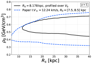
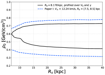
Figure 3: Top panel: 2$\sigma$ contours in the $(R_{s},\rho_{0})$ plane for fixed $\gamma$. The black contour is obtained for fixed $R_{0}$, and profiled over $V_{0}$, $\mathcal{M}_{i}$, $\langle\tau\rangle$ and $\Sigma_{*}$. The blue dashed line is obtained by profiling over $R_{0}$, $\mathcal{M}_{i}$, $\langle\tau\rangle$ and $\Sigma_{*}$, but for fixed $V_{\odot}$ (as calculated in Paper I). Bottom panel: same as left panel but further profiled over $V_{0}$.

4.2 Gaia ranges

Our fiducial range of $V_{0}$ values, i.e. $[218,240]\,\rm km/s$, encompass, on the one hand, estimates found in the literature, and, on the other hand, it coincides with the Gaia range estimate assuming a 5% systematic uncertainty, which is the most pessimistic value considered in [38]. If we rather assume a 2% systematic uncertainty, which is the more optimistic value considered in [38], the Gaia range shrinks to $[224,234]\,\rm km/s$. In figure 4, we show the constraints obtained in the $(R_{s},\rho_{0})$ plane for the two Gaia ranges. Although the $V_{0}$ range is reduced by 50%, the uncertainty on the local DM density remains virtually unchanged. Similarly to what seen above with $R_{0}$, this indicates that the uncertainties on the spatial distribution and normalization of baryons and the large error bars of the RC dominate our determination of the DM distribution in the MW.

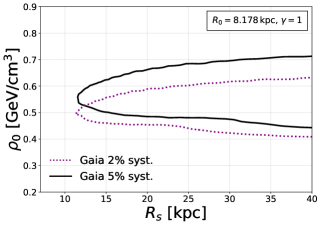
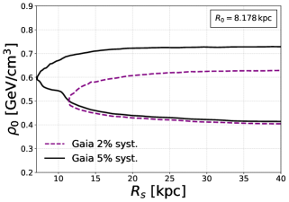
Figure 4: Constraints in the $(R_{s},\rho_{0})$ plane for the two Gaia systematic ranges of $V_{0}$, as explained in the text. Top panel: 2$\sigma$ contours for fixed $\gamma$, profiled over $V_{0}$, $\mathcal{M}_{i}$, $\langle\tau\rangle$ and $\Sigma_{*}$. Bottom panel: same as left panel but further profiled over $\gamma$.

4.3 Comparison with other estimates of $\rho_{0}$ from the literature

In figure 5 we compare the value of $\rho_{0}$ obtained in this work (grey band) with other estimates of this parameter as found in the literature. Our inferred local density ranges at the 1$\sigma$ level are as follows:

$$\begin{split}\rho_{0}&=0.48-$0.67\text{\,}\mathrm{G}\mathrm{e}\mathrm{V}\mathrm{/}\mathrm{c}\mathrm{m}^{3}$\hskip 14.22636pt\textrm{(gNFW)}\\ \rho_{0}&=0.48-$0.67\text{\,}\mathrm{G}\mathrm{e}\mathrm{V}\mathrm{/}\mathrm{c}\mathrm{m}^{3}$\hskip 14.22636pt\textrm{(Einasto)}\\ \rho_{0}&=0.48-$0.69\text{\,}\mathrm{G}\mathrm{e}\mathrm{V}\mathrm{/}\mathrm{c}\mathrm{m}^{3}$\hskip 14.22636pt\textrm{(Burkert)}.\end{split}$$ (5)

Figure 5 includes recent values obtained by global fitting of Galactic mass models to the RC [2, 49, 38, 13, 53, 8, 54, 55] and other techniques, such as fitting of the velocity distribution function, or the application of Jeans equations using global mass models [56, 57, 58, 59]. We have included the two values of $\rho_{0}$ as estimated in [13] adopting two different baryonic mass distributions. We have also included recent estimates using stellar tracers of the local gravitational force [60, 61, 12, 62, 63, 64, 65, 66, 67] and the value recommended in the SHM⁺⁺ [68]. The three yellow bands for [62] and [64] correspond to estimates of $\rho_{0}$ using different populations of stellar tracers. Furthermore, [67] estimated the local gravitational force using stellar tracers in the Northern and Southern hemisphere, also fitting a global model of the Galaxy to both tracers (yellow-and-purple error bar). For a recent review of techniques and estimates of $\rho_{0}$, please see [15].

Figure 5: Recent determinations of $\rho_{0}$ as obtained with the RC technique (purple error bars) and other global methods (blue error bars). The yellow error bars correspond to $\rho_{0}$ values estimated through Jeans modelling of stellar tracers in our Solar neighborhood. The yellow-and-purple error bar is obtained by fitting a global mass model of the Galaxy to local kinematics. Finally, the grey error bar corresponds to the value recommended in the SHM⁺⁺ [68], the GAIA Cepheids^∗ datapoint is from the analysis performed here and presented in D, and the grey band “BIC ’21” is the main result of this work, using the galkin database. Notice that different determinations use different $(R_{0},V_{0})$ and $(U_{\odot},V_{\odot},W_{\odot})$ values. See text in Section 4.3 for further details.

5 Conclusions

We have quantified astrophysical uncertainties on the distribution of Dark Matter in the Milky Way (under the assumption of a gNFW, Burkert and Einasto density profiles) by comparing the observed Rotation Curve with that expected to be caused by the baryonic and DM components of the Galaxy. We have made use of state-of-the-art (AD 2020) estimates of the Galactic parameters $(R_{0},V_{0})$ [69, 38], updating a previous analysis [16] also adopting $V_{0}$ as a new independent variable (instead of $R_{0}$, as in the previous analysis). Our main conclusion is that, despite using the recent precise measurements of $R_{0}$ and $V_{0}$ from the Gravity collaboration and Gaia DR2, respectively, uncertainties on the determination of the DM distribution stay sizable, and comparable with those estimated with earlier determinations of the Galactic parameters, contrary to general expectations prior to data release. This is driven by the fact that the main source of astrophysical uncertainties remains that on the shape and mass of the baryonic component of the Galaxy, and the systematic uncertainties in the observational determination of the Milky Way’s rotation curve.

We infer a local density range $\rho_{0}$=$0.4-0.7\,{\rm GeV/cm^{3}}$ at the 2$\sigma$ level, assuming a generalized NFW (gNFW) profile. This range coincides with that obtained under the assumption of an Einasto and a Burkert density profiles, thus indicating that the choice of profile does not affect the determination of local Dark Matter density, within the astrophysical uncertainties.

We provide both the likelihood profile and the Bayesian posterior of the present analysis – publicly available at the link in this footnote – so to be adopted in BSM searches to include the most relevant astrophysical uncertainties on the determination of the Dark Matter distribution in the Milky Way.

Adopting state-of-the-art (AD 2021) determinations of Galactic parameters, we find in fact that the uncertainties on quantities relevant for searches of the nature of Dark Matter –propagated from those of astrophysical nature– are sizable, and should be properly included in all comprehensive analysis.

Appendix A Burkert profile

In this appendix we present the results obtained for a Burkert profile [30]. The Burkert DM density profile has two free parameters: the core radius $R_{c}$ and the local DM density $\rho_{0}$. In the top panel of figure A.6 we present the 2$\sigma$ contours in the $(R_{c},\rho_{0})$ plane taking into account the latest measurements of the astrophysical quantities $(R_{0},V_{0})$ [69, 38]. In the bottom panel of the same figure, we compare the 2$\sigma$ contour obtained in this work (i.e. $\chi^{2}_{\rm RC}$ profiled over $V_{0}$, $\mathcal{M}_{i}$, $\langle\tau\rangle$ and $\Sigma_{*}$) shown in black, with that obtained in Paper I –obtained by profiling over $R_{0}$, $\mathcal{M}_{i}$, $\langle\tau\rangle$ and $\Sigma_{*}$– which is shown in blue. Due to the reduction on uncertainties on astrophysical quantities, the minimum core size is reduced from 5 kpc to roughly 8 kpc. Furthermore, uncertainties on the local DM density are slightly reduced from $0.33-0.73\,{\rm GeV/cm^{3}}$ to $0.41-0.73\,{\rm GeV/cm^{3}}$. As for the gNFW case, uncertainties on our estimate of the DM distribution in the MW are dominated by our ignorance on the actual shape and weight of the baryonic component of the Galaxy.

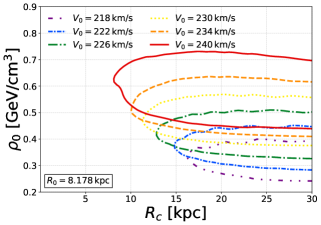
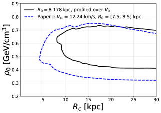
Figure A.6: 2$\sigma$ contours in the ($R_{c}$, $\rho_{0}$) plane for a Burkert profile. Top panel: for various values of $V_{0}$ and profiled over $\mathcal{M}_{i}$, $\langle\tau\rangle$ and $\Sigma_{*}$. Bottom panel: further profiled over $V_{0}$ (black contour), and, in dashed blue, contour obtained in Paper I (profiled over $R_{0}$, $\mathcal{M}_{i}$, $\langle\tau\rangle$ and $\Sigma_{*}$).

Appendix B Einasto profile

We also present the results obtained for an Einasto DM density profile [31], which is defined in terms of the shape parameter (or inner slope of the logarithmic density profile) $\alpha$, the scale radius $R_{s}$ and the local DM density $\rho_{0}$. The left panel of figure B.7 shows the $2\sigma$ contours obtained in the ($R_{s}$, $\rho_{0}$) plane, for different values of the parameter $\alpha$ and profiled over $V_{0}$, $\mathcal{M}_{i}$, $\langle\tau\rangle$ and $\Sigma_{0}$, while taking into account the recent estimations of the Sun’s galactocentric distance and its circular velocity [69, 38]. The right panel of figure B.7 compares the constraints obtained in light of new astrophysical data (black contour) with the results obtained in Paper I (blue contour). In light of new estimates of the Sun’s distance to the GC and its circular velocity, the allowed 2$\sigma$ range for the local DM density is $0.41-0.73\,{\rm GeV/cm^{3}}$.

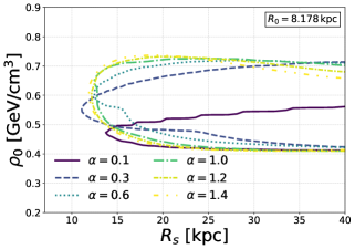
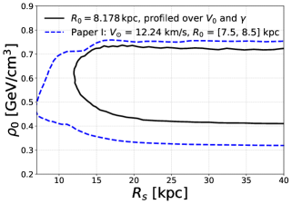
Figure B.7: Constraints in the $(R_{s},\rho_{0})$ for an Einasto profile. Left panel: 2$\sigma$ contours for different values of $\alpha$ and fixed $R_{0}$, profiled over $V_{0}$, $\mathcal{M}_{i}$, $\langle\tau\rangle$ and $\Sigma_{*}$. Right panel: 2$\sigma$ contours for fixed $R_{0}$, profiled over $\alpha$, $V_{0}$, $\mathcal{M}_{i}$, $\langle\tau\rangle$ and $\Sigma_{*}$ (black contour). The blue contour corresponds to the one obtained in Paper I, i.e. $\chi^{2}_{RC}$ profiled over $\alpha$, $R_{0}$, $\mathcal{M}_{i}$, $\langle\tau\rangle$ and $\Sigma_{*}$.

Appendix C Bayesian framework

In this section we present the results of a fully Bayesian analysis. By comparing the results obtained with the frequentist and Bayesian frameworks, we are able to bracket uncertainties due to the use of the statistical methodology. For a given baryonic morphology, our model has six free parameters: the three parameters $(R_{s},\rho_{0},\gamma)$ of the gNFW density profile, the two parameters that control the normalization of the baryonic mass, namely $\langle\tau\rangle$ and $\Sigma_{*}$, and the Sun’s circular velocity $V_{0}$. We perform a Monte Carlo scan of the parameter space by means of the nested sampling code PyMultiNest [70, 71], using flat priors on the parameters. We account for the uncertainty in the choice of baryonic morphology by repeating the scan for each different morphology and then performing a Bayesian model averaging (e.g. [72]). In particular, we follow the prescription described in section 2.4.2 of [7], with the only difference that, in the analysis presented here, $V_{0}$ is a free parameter. In short, this means that 30 different six-dimensional posterior distributions are calculated, one for each baryonic morphology, and then they are averaged to get the final one. The six-dimensional model-averaged posterior can be found at https://github.com/mariabenitocst/UncertaintiesDMinTheMW.

Figure C.8 shows the one and two-dimensional marginalized posterior distributions for the model-averaged. The Bayesian contours (shown in magenta) delimiting regions of 68% and 95% probability are compared with the 1-2 $\sigma$ frequentist contours, which are shown in black. The Bayesian model-averaged contours are less conservative than the frequentist counterparts and thus, as observed in the figure, the former contours are smaller.

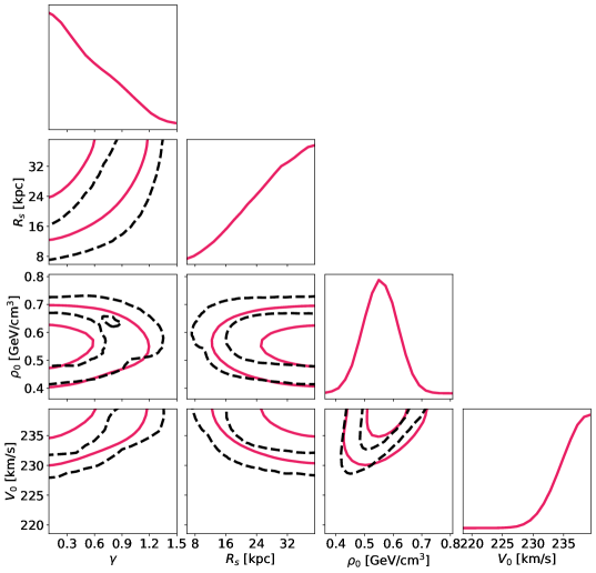
Figure C.8: One and two-dimensional marginalized Bayesian posterior distributions for the baryonic model-averaged case (magenta). The Bayesian contours delimit regions of 68% and 95% probability. The frequentist contours delimiting the 68% and 95% confidence regions are also shown in black. The full posterior is 6-d, but for better clearness, we only show the triangle plot in the four most relevant parameters, i.e., $R_{s},\rho_{0},\gamma$ and $V_{0}$.

Appendix D Cepheids Gaia Rotation Curve

In [73], the authors obtain the RC between 4 and 20 kpc from the Galactic center using classical Cepheids –with proper motions and radial velocities measured by Gaia DR2– as tracers. We wish to investigate the constraints in the Galactic distribution of DM set by this new data, adopting the RC in the data format presented in the aforementioned analysis as it permits the same binning procedure we used for the galkin compilation. For this check, we adopt the Cepheids Gaia RC assuming $R_{0}=$8.09\text{\,}\mathrm{k}\mathrm{p}\mathrm{c}$$ and $V_{0}=$233.6\text{\,}\mathrm{k}\mathrm{m}\mathrm{/}\mathrm{s}$$, which are the values estimated in [73]. We first bin the RC and then, we perform a scan in the 6-dimensional parameter space $(\gamma,r_{s},\rho_{0},\mathcal{M}_{i},\langle\tau\rangle,\Sigma_{*})$ closely following the procedure described in section 2.

Figure D.9 compares the binned RC as obtained from the galkin data set and Cepheids Gaia. Figure D.10 compares the 2$\sigma$ contours obtained for the Cepheids RC with those obtained for the galkin data set. It can be seen that the Cepheids data seem to prefer $\rho_{0}$ values slightly smaller than those preferred by the galkin compilation, while still being in full agreement with each other. It is to be noticed that the Gaia contours are only for a fixed value of $V_{0}$, thus the smaller region obtained should not generate surprise.

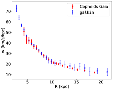
Figure D.9: Binned angular rotation curve for the Cepheids Gaia and galkin data sets with fixed $R_{0}=$8.09\text{\,}\mathrm{k}\mathrm{p}\mathrm{c}$$ and $V_{0}=$233.6\text{\,}\mathrm{k}\mathrm{m}\mathrm{/}\mathrm{s}$$.

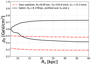
Figure D.10: 2$\sigma$ contours in the $(\gamma,\rho_{0})$ (top panel) and $(R_{s},\rho_{0})$ (bottom panel) planes for the Cepheids Gaia RC (dash-dotted red) and the galkin data set as obtained in this work (solid black). Top panel: contours are profiled over baryonic morphology, normalization and $R_{s}$. The contours obtained for the galkin dataset are further profiled over $V_{0}$.

References

- [1] F. Iocco, M. Pato, G. Bertone, Evidence for dark matter in the inner Milky Way, Nature Physics 11 (3) (2015) 245–248. arXiv:1502.03821, doi:10.1038/nphys3237.
- [2] M. Pato, F. Iocco, The Dark Matter Profile of the Milky Way: A Non-parametric Reconstruction, The Astrophysical Journal Letters803 (1) (2015) L3. arXiv:1504.03317, doi:10.1088/2041-8205/803/1/L3.
- [3] J. Bovy, H.-W. Rix, A Direct Dynamical Measurement of the Milky Way’s Disk Surface Density Profile, Disk Scale Length, and Dark Matter Profile at 4 kpc <~R <~9 kpc, The Astrophysical Journal779 (2) (2013) 115. arXiv:1309.0809, doi:10.1088/0004-637X/779/2/115.
- [4] M. Pato, F. Iocco, G. Bertone, Dynamical constraints on the dark matter distribution in the Milky Way, JCAP2015 (12) (2015) 001. arXiv:1504.06324, doi:10.1088/1475-7516/2015/12/001.
- [5] F. Iocco, M. Benito, An estimate of the DM profile in the Galactic bulge region, Physics of the Dark Universe 15 (2017) 90–95. arXiv:1611.09861, doi:10.1016/j.dark.2016.12.004.
- [6] M. Benito, N. Bernal, N. Bozorgnia, F. Calore, F. Iocco, Particle Dark Matter constraints: the effect of Galactic uncertainties, JCAP2017 (2) (2017) 007. arXiv:1612.02010, doi:10.1088/1475-7516/2017/02/007.
- [7] E. V. Karukes, M. Benito, F. Iocco, R. Trotta, A. Geringer-Sameth, A robust estimate of the Milky Way mass from rotation curve data, JCAP2020 (5) (2020) 033. arXiv:1912.04296, doi:10.1088/1475-7516/2020/05/033.
- [8] E. V. Karukes, M. Benito, F. Iocco, R. Trotta, A. Geringer-Sameth, Bayesian reconstruction of the Milky Way dark matter distribution, JCAP2019 (9) (2019) 046. arXiv:1901.02463, doi:10.1088/1475-7516/2019/09/046.
- [9] F. Nesti, P. Salucci, The Dark Matter halo of the Milky Way, AD 2013, JCAP 1307 (2013) 016. arXiv:1304.5127, doi:10.1088/1475-7516/2013/07/016.
- [10] H. Silverwood, S. Sivertsson, P. Steger, J. I. Read, G. Bertone, A non-parametric method for measuring the local dark matter density, Mon. Not. Roy. Astron. Soc. 459 (4) (2016) 4191–4208. arXiv:1507.08581, doi:10.1093/mnras/stw917.
- [11] R. Catena, P. Ullio, A novel determination of the local dark matter density, JCAP 1008 (2010) 004. arXiv:0907.0018, doi:10.1088/1475-7516/2010/08/004.
- [12] S. Sivertsson, H. Silverwood, J. I. Read, G. Bertone, P. Steger, The local dark matter density from SDSS-SEGUE G-dwarfs, MNRAS478 (2) (2018) 1677–1693. arXiv:1708.07836, doi:10.1093/mnras/sty977.
- [13] P. F. de Salas, K. Malhan, K. Freese, K. Hattori, M. Valluri, On the estimation of the local dark matter density using the rotation curve of the Milky Way, JCAP2019 (10) (2019) 037. arXiv:1906.06133, doi:10.1088/1475-7516/2019/10/037.
- [14] A. Widmark, K. Malhan, P. F. de Salas, S. Sivertsson, Measuring the Matter Density of the Galactic Disk Using Stellar Streams, MNRAS(Jun. 2020). arXiv:2003.04318, doi:10.1093/mnras/staa1741.
- [15] P. F. de Salas, A. Widmark, Dark matter local density determination: recent observations and future prospects, arXiv e-prints (2020) arXiv:2012.11477arXiv:2012.11477.
- [16] M. Benito, A. Cuoco, F. Iocco, Handling the uncertainties in the Galactic Dark Matter distribution for particle Dark Matter searches, JCAP2019 (3) (2019) 033. arXiv:1901.02460, doi:10.1088/1475-7516/2019/03/033.
- [17] Y. Farzan, M. Rajaee, Dark matter decaying into millicharged particles as a solution to AMS-02 positron excess, JCAP2019 (4) (2019) 040. arXiv:1901.11273, doi:10.1088/1475-7516/2019/04/040.
- [18] J. F. Acevedo, J. Bramante, Supernovae sparked by dark matter in white dwarfs, Phys. Rev. D100 (4) (2019) 043020. arXiv:1904.11993, doi:10.1103/PhysRevD.100.043020.
- [19] S.-J. Lin, X.-J. Bi, P.-F. Yin, Investigating the dark matter signal in the cosmic ray antiproton flux with the machine learning method, Phys. Rev. D100 (10) (2019) 103014. arXiv:1903.09545, doi:10.1103/PhysRevD.100.103014.
- [20] C. A. Argüelles, A. Diaz, A. Kheirandish, et al., Dark Matter Annihilation to Neutrinos: An Updated, Consistent & Compelling Compendium of Constraints, arXiv e-prints (2019) arXiv:1912.09486arXiv:1912.09486.
- [21] J. S. Sidhu, Charge constraints of macroscopic dark matter, Phys. Rev. D101 (4) (2020) 043526. arXiv:1912.04732, doi:10.1103/PhysRevD.101.043526.
- [22] ANTARES Collaboration, A. Albert, M. André, M. Anghinolfi, et al., Combined search for neutrinos from dark matter self-annihilation in the Galactic Centre with ANTARES and IceCube, arXiv e-prints (2020) arXiv:2003.06614arXiv:2003.06614.
- [23] G. Baym, D. H. Beck, J. P. Filippini, C. J. Pethick, J. Shelton, Searching for low mass dark matter via phonon creation in superfluid 4He, arXiv e-prints (2020) arXiv:2005.08824arXiv:2005.08824.
- [24] G. B. Gelmini, A. J. Millar, V. Takhistov, E. Vitagliano, Probing Dark Photons with Plasma Haloscopes, arXiv e-prints (2020) arXiv:2006.06836arXiv:2006.06836.
- [25] T. Bringmann, M. Pospelov, Novel Direct Detection Constraints on Light Dark Matter, Phys. Rev. Letters122 (17) (2019) 171801. arXiv:1810.10543, doi:10.1103/PhysRevLett.122.171801.
- [26] M. Pato, F. Iocco, galkin: A new compilation of Milky Way rotation curve data, SoftwareX 6 (2017) 54–62. arXiv:1703.00020, doi:10.1016/j.softx.2016.12.006.
- [27] R. Drimmel, E. Poggio, On the Solar Velocity, Research Notes of the American Astronomical Society 2 (4) (2018) 210. doi:10.3847/2515-5172/aaef8b.
- [28] H. Zhao, Analytical models for galactic nuclei, MNRAS278 (2) (1996) 488–496. arXiv:astro-ph/9509122, doi:10.1093/mnras/278.2.488.
- [29] J. S. B. Wyithe, E. L. Turner, D. N. Spergel, Gravitational Lens Statistics for Generalized NFW Profiles: Parameter Degeneracy and Implications for Self-Interacting Cold Dark Matter, The Astrophysical Journal555 (1) (2001) 504–523. arXiv:astro-ph/0007354, doi:10.1086/321437.
-
[30]
A. Burkert, The structure of dark
matter halos in dwarf galaxies, The Astrophysical Journal 447 (1) (Jul
1995).
doi:10.1086/309560.
URL http://dx.doi.org/10.1086/309560 - [31] J. Einasto, On the Construction of a Composite Model for the Galaxy and on the Determination of the System of Galactic Parameters, Trudy Astrofizicheskogo Instituta Alma-Ata 5 (1965) 87–100.
- [32] P. Popowski, K. Griest, C. L. Thomas, et al., Microlensing Optical Depth toward the Galactic Bulge Using Clump Giants from the MACHO Survey, The Astrophysical Journal631 (2) (2005) 879–905. arXiv:astro-ph/0410319, doi:10.1086/432246.
- [33] Gravity Collaboration, R. Abuter, A. Amorim, M. Bauböck, et al., A geometric distance measurement to the Galactic center black hole with 0.3% uncertainty, Astron. Astrophys.625 (2019) L10. arXiv:1904.05721, doi:10.1051/0004-6361/201935656.
- [34] Gaia Collaboration, T. Prusti, J. H. J. de Bruijne, A. G. A. Brown, et al., The Gaia mission, Astron. Astrophys.595 (2016) A1. arXiv:1609.04153, doi:10.1051/0004-6361/201629272.
- [35] E. L. Wright, P. R. M. Eisenhardt, A. K. Mainzer, et al., The Wide-field Infrared Survey Explorer (WISE): Mission Description and Initial On-orbit Performance, Astronomic. J.140 (6) (2010) 1868–1881. arXiv:1008.0031, doi:10.1088/0004-6256/140/6/1868.
- [36] M. F. Skrutskie, R. M. Cutri, R. Stiening, et al., The Two Micron All Sky Survey (2MASS), Astronomic. J.131 (2) (2006) 1163–1183. doi:10.1086/498708.
- [37] S. R. Majewski, R. P. Schiavon, P. M. Frinchaboy, et al., The Apache Point Observatory Galactic Evolution Experiment (APOGEE), Astronomic. J.154 (3) (2017) 94. arXiv:1509.05420, doi:10.3847/1538-3881/aa784d.
- [38] A.-C. Eilers, D. W. Hogg, H.-W. Rix, M. K. Ness, The Circular Velocity Curve of the Milky Way from 5 to 25 kpc, The Astrophysical Journal871 (1) (2019) 120. arXiv:1810.09466, doi:10.3847/1538-4357/aaf648.
- [39] GRAVITY Collaboration, R. Abuter, A. Amorim, M. Bauboeck, et al., Detection of the Schwarzschild precession in the orbit of the star S2 near the Galactic centre massive black hole, arXiv e-prints (2020) arXiv:2004.07187arXiv:2004.07187.
- [40] J. Bovy, C. Allende Prieto, T. C. Beers, et al., The Milky Way’s Circular-velocity Curve between 4 and 14 kpc from APOGEE data, The Astrophysical Journal759 (2) (2012) 131. arXiv:1209.0759, doi:10.1088/0004-637X/759/2/131.
- [41] M. J. Reid, K. M. Menten, A. Brunthaler, et al., Trigonometric Parallaxes of High Mass Star Forming Regions: The Structure and Kinematics of the Milky Way, The Astrophysical Journal783 (2) (2014) 130. arXiv:1401.5377, doi:10.1088/0004-637X/783/2/130.
- [42] J. Bland-Hawthorn, O. Gerhard, The Galaxy in Context: Structural, Kinematic, and Integrated Properties, Annu. Rev. Astron. Astrophys.54 (2016) 529–596. arXiv:1602.07702, doi:10.1146/annurev-astro-081915-023441.
- [43] R. Schönrich, Galactic rotation and solar motion from stellar kinematics, MNRAS427 (1) (2012) 274–287. arXiv:1207.3079, doi:10.1111/j.1365-2966.2012.21631.x.
- [44] A. S. Stepanishchev, V. V. Bobylev, Galactic rotation curve from the space velocities of selected masers, Astronomy Letters 37 (4) (2011) 254–266. doi:10.1134/S1063773711030054.
- [45] S. E. Koposov, H.-W. Rix, D. W. Hogg, Constraining the Milky Way Potential with a Six-Dimensional Phase-Space Map of the GD-1 Stellar Stream, The Astrophysical Journal712 (1) (2010) 260–273. arXiv:0907.1085, doi:10.1088/0004-637X/712/1/260.
- [46] D. W. Hogg, M. R. Blanton, S. T. Roweis, K. V. Johnston, Modeling Complete Distributions with Incomplete Observations: The Velocity Ellipsoid from Hipparcos Data, The Astrophysical Journal629 (1) (2005) 268–275. arXiv:astro-ph/0505057, doi:10.1086/431572.
- [47] R. Schönrich, J. Binney, W. Dehnen, Local kinematics and the local standard of rest, MNRAS403 (4) (2010) 1829–1833. arXiv:0912.3693, doi:10.1111/j.1365-2966.2010.16253.x.
- [48] H.-J. Tian, C. Liu, J. L. Carlin, Y.-H. Zhao, X.-L. Chen, Y. Wu, G.-W. Li, Y.-H. Hou, Y. Zhang, The Stellar Kinematics in the Solar Neighborhood from LAMOST Data, The Astrophysical Journal809 (2) (2015) 145. arXiv:1507.05624, doi:10.1088/0004-637X/809/2/145.
- [49] Y. Huang, X. W. Liu, H. B. Yuan, et al., Determination of the local standard of rest using the LSS-GAC DR1, MNRAS449 (1) (2015) 162–174. arXiv:1501.07095, doi:10.1093/mnras/stv204.
- [50] S. Sharma, J. Bland-Hawthorn, J. Binney, et al., Kinematic Modeling of the Milky Way Using the RAVE and GCS Stellar Surveys, The Astrophysical Journal793 (1) (2014) 51. arXiv:1405.7435, doi:10.1088/0004-637X/793/1/51.
- [51] J. Bovy, J. C. Bird, A. E. García Pérez, S. R. Majewski, D. L. Nidever, G. Zasowski, The Power Spectrum of the Milky Way: Velocity Fluctuations in the Galactic Disk, The Astrophysical Journal800 (2) (2015) 83. arXiv:1410.8135, doi:10.1088/0004-637X/800/2/83.
- [52] M. J. Reid, A. Brunthaler, The Proper Motion of Sagittarius A*. II. The Mass of Sagittarius A*, The Astrophysical Journal616 (2) (2004) 872–884. arXiv:astro-ph/0408107, doi:10.1086/424960.
- [53] H.-N. Lin, X. Li, The dark matter profiles in the Milky Way, MNRAS487 (4) (2019) 5679–5684. arXiv:1906.08419, doi:10.1093/mnras/stz1698.
- [54] M. Cautun, A. Benítez-Llambay, A. J. Deason, et al., The milky way total mass profile as inferred from Gaia DR2, MNRAS494 (3) (2020) 4291–4313. arXiv:1911.04557, doi:10.1093/mnras/staa1017.
- [55] Y. Sofue, Rotation Curve of the Milky Way and the Dark Matter Density, Galaxies 8 (2) (2020) 37. arXiv:2004.11688, doi:10.3390/galaxies8020037.
- [56] D. R. Cole, J. Binney, A centrally heated dark halo for our Galaxy, MNRAS465 (1) (2017) 798–810. arXiv:1610.07818, doi:10.1093/mnras/stw2775.
- [57] P. J. McMillan, The mass distribution and gravitational potential of the Milky Way, MNRAS465 (1) (2017) 76–94. arXiv:1608.00971, doi:10.1093/mnras/stw2759.
- [58] C. Wegg, O. Gerhard, M. Bieth, The gravitational force field of the Galaxy measured from the kinematics of RR Lyrae in Gaia, MNRAS485 (3) (2019) 3296–3316. arXiv:1806.09635, doi:10.1093/mnras/stz572.
- [59] K. Hattori, M. Valluri, E. Vasiliev, Action-based distribution function modelling for constraining the shape of the Galactic dark matter halo, arXiv e-prints (2020) arXiv:2012.03908arXiv:2012.03908.
- [60] C. F. McKee, A. Parravano, D. J. Hollenbach, Stars, Gas, and Dark Matter in the Solar Neighborhood, The Astrophysical Journal814 (1) (2015) 13. arXiv:1509.05334, doi:10.1088/0004-637X/814/1/13.
- [61] Q. Xia, C. Liu, S. Mao, Y. Song, L. Zhang, R. J. Long, Y. Zhang, Y. Hou, Y. Wang, Y. Wu, Determining the local dark matter density with LAMOST data, MNRAS458 (4) (2016) 3839–3850. arXiv:1510.06810, doi:10.1093/mnras/stw565.
- [62] K. Schutz, T. Lin, B. R. Safdi, C.-L. Wu, Constraining a Thin Dark Matter Disk with G a i a, Phys. Rev. Letters121 (8) (2018) 081101. arXiv:1711.03103, doi:10.1103/PhysRevLett.121.081101.
- [63] J. H. J. Hagen, A. Helmi, The vertical force in the solar neighbourhood using red clump stars in TGAS and RAVE. Constraints on the local dark matter density, Astron. Astrophys.615 (2018) A99. arXiv:1802.09291, doi:10.1051/0004-6361/201832903.
- [64] J. Buch, J. S. C. Leung, J. Fan, Using Gaia DR2 to constrain local dark matter density and thin dark disk, JCAP2019 (4) (2019) 026. arXiv:1808.05603, doi:10.1088/1475-7516/2019/04/026.
- [65] M. S. Nitschai, M. Cappellari, N. Neumayer, First Gaia dynamical model of the Milky Way disc with six phase space coordinates: a test for galaxy dynamics, MNRAS494 (4) (2020) 6001–6011. arXiv:1909.05269, doi:10.1093/mnras/staa1128.
- [66] R. Guo, C. Liu, S. Mao, X.-X. Xue, R. J. Long, L. Zhang, Measuring the local dark matter density with LAMOST DR5 and Gaia DR2, MNRAS495 (4) (2020) 4828–4844. arXiv:2005.12018, doi:10.1093/mnras/staa1483.
- [67] J.-B. Salomon, O. Bienaymé, C. Reylé, A. C. Robin, B. Famaey, Kinematics and dynamics of Gaia red clump stars. Revisiting north-south asymmetries and dark matter density at large heights, Astron. Astrophys.643 (2020) A75. arXiv:2009.04495, doi:10.1051/0004-6361/202038535.
- [68] N. W. Evans, C. A. J. O’Hare, C. McCabe, SHM++: A Refinement of the Standard Halo Model for Dark Matter Searches in Light of the Gaia Sausage, arXiv e-prints (2018) arXiv:1810.11468arXiv:1810.11468.
- [69] R. Abuter, et al., Detection of the gravitational redshift in the orbit of the star S2 near the Galactic centre massive black hole, Astron. Astrophys. 615 (2018) L15. arXiv:1807.09409, doi:10.1051/0004-6361/201833718.
- [70] F. Feroz, M. P. Hobson, M. Bridges, MULTINEST: an efficient and robust Bayesian inference tool for cosmology and particle physics, MNRAS398 (4) (2009) 1601–1614. arXiv:0809.3437, doi:10.1111/j.1365-2966.2009.14548.x.
- [71] J. Buchner, A. Georgakakis, K. Nandra, et al., X-ray spectral modelling of the AGN obscuring region in the CDFS: Bayesian model selection and catalogue, Astron. Astrophys.564 (2014) A125. arXiv:1402.0004, doi:10.1051/0004-6361/201322971.
- [72] R. Trotta, Bayes in the sky: Bayesian inference and model selection in cosmology, Contemporary Physics 49 (2) (2008) 71–104. arXiv:0803.4089, doi:10.1080/00107510802066753.
- [73] P. Mróz, A. Udalski, D. M. Skowron, J. Skowron, I. Soszyński, P. Pietrukowicz, M. K. Szymański, R. Poleski, S. Kozłowski, K. Ulaczyk, Rotation Curve of the Milky Way from Classical Cepheids, The Astrophysical Journal Letters870 (1) (2019) L10. arXiv:1810.02131, doi:10.3847/2041-8213/aaf73f.
Acknowledgements
M. B. is supported by the ERDF Centre of Excellence project TK133 and the Estonian Research Council PRG803 grant. F. I.’s work has been partially supported by the research grant number 2017W4HA7S “NAT-NET: Neutrino and Astroparticle Theory Network” under the program PRIN 2017 funded by the Italian Ministero dell’Università e della Ricerca (MUR). Numerical resources for this research have been supplied by the Center for Scientific Computing (NCC/GridUNESP) of the São Paulo State University (UNESP). A.C. is supported by: ‘Departments of Excellence 2018-2022” grant awarded by the Italian Ministry of Education, University and Research (MIUR) L. 232/2016; Research grant “The Dark Universe: A Synergic Multimessenger Approach” No. 2017X7X85K funded by MIUR; Research grant TAsP (Theoretical Astroparticle Physics) funded by INFN.