A Diagnostic Study of Explainability Techniques for Text Classification

Abstract

Recent developments in machine learning have introduced models that approach human performance at the cost of increased architectural complexity. Efforts to make the rationales behind the models’ predictions transparent have inspired an abundance of new explainability techniques. Provided with an already trained model, they compute saliency scores for the words of an input instance. However, there exists no definitive guide on (i) how to choose such a technique given a particular application task and model architecture, and (ii) the benefits and drawbacks of using each such technique. In this paper, we develop a comprehensive list of diagnostic properties for evaluating existing explainability techniques. We then employ the proposed list to compare a set of diverse explainability techniques on downstream text classification tasks and neural network architectures. We also compare the saliency scores assigned by the explainability techniques with human annotations of salient input regions to find relations between a model’s performance and the agreement of its rationales with human ones. Overall, we find that the gradient-based explanations perform best across tasks and model architectures, and we present further insights into the properties of the reviewed explainability techniques.

1 Introduction

Figure 1: Example of the saliency scores for the words (columns) of an instance from the Twitter Sentiment Extraction dataset. They are produced by the explainability techniques (rows) given a $\mathtt{Transformer}$ model. The first row is the human annotation of the salient words. The scores are normalized in the range $[0,1]$.

Understanding the rationales behind models’ decisions is becoming a topic of pivotal importance, as both the architectural complexity of machine learning models and the number of their application domains increases. Having greater insight into the models’ reasons for making a particular prediction has already proven to be essential for discovering potential flaws or biases in medical diagnosis Caruana et al. (2015) and judicial sentencing Rich (2016). In addition, European law has mandated “the right $\dots$ to obtain an explanation of the decision reached”  Regulation (2016).

Explainability methods attempt to reveal the reasons behind a model’s prediction for a single data point, as shown in Figure 1. They can be produced post-hoc, i.e., with already trained models. Such post-hoc explanation techniques can be applicable to one specific model Martens et al. (2008); Wagner et al. (2019) or to a broader range thereof Ribeiro et al. (2016); Lundberg and Lee (2017). They can further be categorised as: employing model gradients Sundararajan et al. (2017); Simonyan et al. (2013), being perturbation based Shapley (1953); Zeiler and Fergus (2014) or providing explanations through model simplifications Ribeiro et al. (2016); Johansson et al. (2004). There also exist explainability methods that generate textual explanations Camburu et al. (2018) and are trained post-hoc or jointly with the model at hand.

While there is a growing amount of explainability methods, we find that they can produce varying, sometimes contradicting explanations, as illustrated in Figure 1. Hence, it is important to assess existing techniques and to provide a generally applicable and automated methodology for choosing one that is suitable for a particular model architecture and application task Jacovi and Goldberg (2020). Robnik-Šikonja and Bohanec (2018) compiles a list of property definitions for explainability techniques, but it remains a challenge to evaluate them in practice. Several other studies have independently proposed different setups for probing varied aspects of explainability techniques DeYoung et al. (2020); Sundararajan et al. (2017). However, existing studies evaluating explainability methods are discordant and do not compare to properties from previous studies. In our work, we consider properties from related work and extend them to be applicable to a broader range of downstream tasks.

Furthermore, to create a thorough setup for evaluating explainability methods, one should include at least: (i) different groups of explainability methods (explanation by simplification, gradient-based, etc.), (ii) different downstream tasks, and (iii) different model architectures. However, existing studies usually consider at most two of these aspects, thus providing insights tied to a specific setup.

We propose a number of diagnostic properties for explainability methods and evaluate them in a comparative study. We consider explainability methods from different groups, all widely applicable to most ML models and application tasks. We conduct an evaluation on three text classification tasks, which contain human annotations of salient tokens. Such annotations are available for Natural Language Processing (NLP) tasks, as they are relatively easy to obtain. This is in contrast to ML sub-fields such as image analysis, for which we only found one relevant dataset – 536 manually annotated object bounding boxes for Visual Question Answering Subramanian et al. (2020).

We further compare explainability methods across three of the most widely used model architectures – $\mathtt{CNN}$, $\mathtt{LSTM}$, and $\mathtt{Transformer}$. The $\mathtt{Transformer}$ model achieves state-of-the-art performance on many text classification tasks but has a complex architecture, hence methods to explain its predictions are strongly desirable. The proposed properties can also be directly applied to Machine Learning (ML) subfields other than NLP. The code for the paper is publicly available.
In summary, the contributions of this work are:

• We compile a comprehensive list of diagnostic properties for explainability and automatic measurement of them, allowing for their effective assessment in practice.

• We study and compare the characteristics of different groups of explainability techniques in three different application tasks and three different model architectures.

• We study the attributions of the explainability techniques and human annotations of salient regions to compare and contrast the rationales of humans and machine learning models.

2 Related Work

Explainability methods can be divided into explanations by simplification, e.g., LIME Ribeiro et al. (2016); gradient-based explanations Sundararajan et al. (2017); perturbation-based explanations Shapley (1953); Zeiler and Fergus (2014). Some studies propose the generation of text serving as an explanation, e.g., Camburu et al. (2018); Lei et al. (2016); Atanasova et al. (2020a). For extensive overviews of existing explainability approaches, see Arrieta et al. (2020).

Explainability methods provide explanations of different qualities, so assessing them systematically is pivotal. A common attempt to reveal shortcomings in explainability techniques is to reveal a model’s reasoning process with counter-examples Alvarez-Melis and Jaakkola (2018); Kindermans et al. (2019); Atanasova et al. (2020b), finding different explanations for the same output. However, single counter-examples do not provide a measure to evaluate explainability techniques Jacovi and Goldberg (2020).

Another group of studies performs human evaluation of the outputs of explainability methods Lertvittayakumjorn and Toni (2019); Narayanan et al. (2018). Such studies exhibit low inter-annotator agreement and reflect mostly what appears to be reasonable and appealing to the annotators, not the actual properties of the method.

The most related studies to our work design measures and properties of explainability techniques. Robnik-Šikonja and Bohanec (2018) propose an extensive list of properties. The Consistency property captures the difference between explanations of different models that produce the same prediction; and the Stability property measures the difference between the explanations of similar instances given a single model. We note that similar predictions can still stem from different reasoning paths. Instead, we propose to explore instance activations, which reveal more of the model’s reasoning process than just the final prediction. The authors propose other properties as well, which we find challenging to apply in practice. We construct a comprehensive list of diagnostic properties tied with measures that assess the degree of each characteristic.

Another common approach to evaluate explainability methods is to measure the sufficiency of the most salient tokens for predicting the target label DeYoung et al. (2020). We also include a sufficiency estimate, but instead of fixing a threshold for the tokens to be removed, we measure the decrease of a model’s performance, varying the proportion of excluded tokens. Other perturbation-based evaluation studies and measures exist Sundararajan et al. (2017); Adebayo et al. (2018), but we consider the above, as it is the most widely applied.

Another direction of explainability evaluation is to compare the agreement of salient words annotated by humans to the saliency scores assigned by explanation techniques DeYoung et al. (2020). We also consider the latter and further study the agreement across model architectures, downstream tasks, and explainability methods. While we consider human annotations at the word level Camburu et al. (2018); Lei et al. (2016), there are also datasets Clark et al. (2019); Khashabi et al. (2018) with annotations at the sentence-level, which would require other model architectures, so we leave this for future work.

Existing studies for evaluating explainability heavily differ in their scope. Some concentrate on a single model architecture - BERT-LSTM DeYoung et al. (2020), RNN Arras et al. (2019), CNN Lertvittayakumjorn and Toni (2019), whereas a few consider more than one model Guan et al. (2019); Poerner et al. (2018). Some studies concentrate on one particular dataset Guan et al. (2019); Arras et al. (2019), while only a few generalize their findings over downstream tasks DeYoung et al. (2020); Vashishth et al. (2019). Finally, existing studies focus on one Vashishth et al. (2019) or a single group of explainability methods DeYoung et al. (2020); Adebayo et al. (2018). Our study is the first to propose a unified comparison of different groups of explainability techniques across three text classification tasks and three model architectures.

3 Evaluating Attribution Maps

We now define a set of diagnostic properties of explainability techniques, and propose how to quantify them. Similar notions can be found in related work Robnik-Šikonja and Bohanec (2018); DeYoung et al. (2020), and we extend them to be generally applicable to downstream tasks. We first introduce the prerequisite notation. Let $X=\{(x_{i},y_{i},w_{i})|i\in[1,N]\}$ be the test dataset, where each instance consists of a list of tokens $x_{i}$ = $\{x_{i,j}|j\in[1,|x_{i}|]\}$, a gold label $y_{i}$, and a gold saliency score for each of the tokens in $x_{i}$: $w_{i}=\{w_{i,j}|j\in[1,|x_{i}|]\}$ with each $w_{i,j}\in\{0,1\}$. Let $\omega$ be an explanation technique that, given a model $M$, a class $c$, and a single instance $x_{i}$, computes saliency scores for each token in the input: $\omega_{x_{i},c}^{M}$$=\{\omega_{(i,j),c}^{M}|j\in[1,|x_{i}|]\}$. Finally, let $M=M_{1},\dots M_{K}$ be models with the same architecture, each trained from a randomly chosen seed, and let $M^{\prime}=M_{1}^{\prime},\dots M_{K}^{\prime}$ be models of the same architecture, but with randomly initialized weights.

Agreement with human rationales (HA). This diagnostic property measures the degree of overlap between saliency scores provided by human annotators, specific to the particular task, and the word saliency scores computed by an explainability technique on each instance. The property is a simple way of approximating the quality of the produced feature attributions. While it does not necessarily mean that the saliency scores explain the predictions of a model, we assume that explanations with high agreement scores would be more comprehensible for the end-user as they would adhere more to human reasoning. With this diagnostic property, we can also compare how the type and the performance of a model and/or dataset affect the agreement with human rationales when observing one type of explainability technique.

During evaluation, we provide an estimate of the average agreement of the explainability technique across the dataset. To this end, we start at the instance level and compute the Average Precision (AP) of produced saliency scores $\omega_{x_{i},c}^{M}$ by comparing them to the gold saliency annotations $w_{i}$. Here, the label for computing the saliency scores is the gold label: $c=y_{i}$. Then, we compute the average across all instances, arriving at Mean AP (MAP):

$$\textrm{MAP}(\omega,M,X)=\frac{1}{N}\sum\limits_{i\in[1,N]}AP(w_{i},\omega_{x_{i},y_{i}}^{M})$$ (1)

Confidence Indication (CI). A token from a single instance can receive several saliency scores, indicating its contribution to the prediction of each of the classes. Thus, when a model recognizes a highly indicative pattern of the predicted class $k$, the tokens involved in the pattern would have highly positive saliency scores for this class and highly negative saliency scores for the remaining classes. On the other hand, when the model is not highly confident, we can assume that it is unable to recognize a strong indication of any class, and the tokens accordingly do not have high saliency scores for any class. Thus, the computed explanation of an instance $i$ should indicate the confidence $p_{i,k}$ of the model in its prediction.

We propose to measure the predictive power of the produced explanations for the confidence of the model. We start by computing the Saliency Distance (SD) between the saliency scores for the predicted class $k$ to the saliency scores of the other classes $K/k$ (Eq. 2). Given the distance between the saliency scores, we predict the confidence of the class with logistic regression (LR) and finally compute the Mean Absolute Error – MAE (Eq. 3), of the predicted confidence to the actual one.

$$\textrm{SD}=\sum\limits_{j\in[0,|x|]}D(\omega_{x_{i,j},k}^{M},\omega_{x_{i,j},K/k}^{M})$$ (2)

$$\textrm{MAE}(\omega,M,X)=\sum\limits_{\begin{subarray}{c}i\in[1,N]\end{subarray}}|p_{i,k}-\textrm{LR}(\textrm{SD})|~{}$$ (3)

For tasks with two classes, D is the subtraction of the saliency value for class k and the other class. For more than two classes, D is the concatenation of the max, min, and average across the differences of the saliency value for class k and the other classes. Low MAE indicates that model’s confidence can be easily identified by looking at the produced explanations.

Faithfulness (F). Since explanation techniques are employed to explain model predictions for a single instance, an essential property is that they are faithful to the model’s inner workings and not based on arbitrary choices. A well-established way of measuring this property is by replacing a number of the most-salient words with a mask token DeYoung et al. (2020) and observing the drop in the model’s performance. To avoid choosing an unjustified percentage of words to be perturbed, we produce several dataset perturbations by masking 0, 10, 20, …, 100% of the tokens in order of decreasing saliency, thus arriving at $X^{\omega^{0}}$, $X^{\omega^{10}}$, …, $X^{\omega^{100}}$. Finally, to produce a single number to measure faithfulness, we compute the area under the threshold-performance curve (AUC-TP):

$$\textrm{AUC-TP}(\omega,M,X)=$$ (4)

$$\textrm{AUC}([(i,P(M(X^{\omega^{0}}))-M(X^{\omega^{i}}))])$$

where P is a task specific performance measure and $i\in[0,10,\dots,100]$. We also compare the AUC-TP of the saliency methods to a random saliency map to find whether there are explanation techniques producing saliency scores without any contribution over a random score.

Using AUC-TP, we perform an ablation analysis which is a good approximation of whether the most salient words are also the most important ones for a model’s prediction. However, some prior studies Feng et al. (2018) find that models remain confident about their prediction even after stripping most input tokens, leaving a few that might appear nonsensical to humans. The diagnostic properties that follow aim to facilitate a more in-depth analysis of the alignment between the inner workings of a model and produced saliency maps.

Rationale Consistency (RC). A desirable property of an explainability technique is to be consistent with the similarities in the reasoning paths of several models on a single instance. Thus, when two reasoning paths are similar, the scores provided by an explainability technique $\omega$ should also be similar, and vice versa. Note that we are interested in similar reasoning paths as opposed to similar predictions, as the latter does not guarantee analogous model rationales. For models with diverse architectures, we expect rationales to be diverse as well and to cause low consistency. Therefore, we focus on a set of models with the same architecture, trained from different random seeds as well as the same architecture, but with randomly initialized weights. The latter would ensure that we can have model pairs $(M_{s},M_{p})$ with similar and distant rationales. We further claim that the similarity in the reasoning paths could be measured effectively with the distance between the activation maps (averaged across layers and neural nodes) produced by two distinct models (Eq. 5). The distance between the explanation scores is computed simply by subtracting the two (Eq. 6). Finally, we compute Spearman’s $\rho$ between the similarity of the explanation scores and the similarity of the attribution maps (Eq. 7).

$$D(M_{s},M_{p},x_{i})=D(M_{s}(x_{i}),M_{p}(x_{i}))$$ (5)

$$D(M_{s},M_{p},x_{i},\omega)=D(\omega_{x_{i},y_{i}}^{M_{s}},\omega_{x_{i},y_{i}}^{M_{p}})$$ (6)

$$\begin{split}\rho(M_{s},M_{p},X,\omega)=\rho(D(M_{s},M_{p},x_{i}),\\ D(M_{s},M_{p},x_{i},\omega)|i\in[1,N])\end{split}$$ (7)

The higher the positive correlation is, the more consistent the attribution method would be. We choose Spearman’s $\rho$ as it measures the monotonic correlation between the two variables. On the other hand, Pearson’s $\rho$ measures only the linear correlation, and we can have a non-linear correlation between the activation difference and the saliency score differences. When subtracting saliency scores and layer activations, we also take the absolute value of the vector difference as the property should be invariant to order of subtraction. An additional benefit of the property is that low correlation scores would also help to identify explainability techniques that are not faithful to a model’s rationales.

Dataset Consistency (DC). The next diagnostic property is similar to the above notion of rationale consistency but focuses on consistency across instances of a dataset as opposed to consistency across different models of the same architecture. In this case, we test whether instances with similar rationales also receive similar explanations. While Rationale Consistency compares instance explanations of the same instance for different model rationales, Dataset Consistency compares explanations for pairs of instances on the same model. We again measure the similarity between instances $x_{i}$ and $x_{j}$ by comparing their activation maps, as in Eq. 8. The next step is to measure the similarity of the explanations produced by an explainability technique $\omega$, which is the difference between the saliency scores as in Eq. 9. Finally, we measure Spearman’s $\rho$ between the similarity in the activations and the saliency scores as in Eq. 10. We again take the absolute value of the difference.

$$D(M,x_{i},x_{j})=D(M(x_{i}),M(x_{j}))$$ (8)

$$D(M,x_{i},x_{j},\omega)=D(\omega_{x_{i},y_{i}}^{M},\omega_{x_{j},y_{i}}^{M})$$ (9)

$$\begin{split}\rho(M,X,\omega)=\rho(D(M,x_{i},x_{j}),\\ D(M,x_{i},x_{j},\omega)|i,j\in[1,N])\end{split}$$ (10)

4 Experiments

4.1 Datasets

Dataset	Example	Size	Length
e-SNLI Camburu et al. (2018)	Premise: An adult dressed in black holds a stick. Hypothesis: An adult is walking away, empty-handed. Label: contradiction	549 367 Train 9 842 Dev 9 824 Test	27.4 inst. 5.3 expl.
Movie Reviews Zaidan et al. (2007)	Review: he is one of the most exciting martial artists on the big screen, continuing to perform his own stunts and dazzling audiences with his flashy kicks and punches. Class: Positive	1 399 Train 199 Dev 199 Test	834.9 inst. 56.18 expl.
Tweet Sentiment Extraction (TSE)	Tweet: im soo bored…im deffo missing my music channels Class: Negative	21 983 Train 2 747 Dev 2 748 Test	20.5 inst. 9.99 expl.

Table 1: Datasets with human-annotated saliency explanations. The Size column presents the dataset split sizes we use in our experiments. The Length column presents the average number of instance tokens in the test set (inst.) and the average number of human annotated explanation tokens (expl.).

Table 1 provides an overview of the used datasets. For e-SNLI, models predict inference – contradiction, neutral, or entailment – between sentence tuples. For the Movie Reviews dataset, models predict the sentiment – positive, negative, or neutral – of reviews with multiple sentences. Finally, for the TSE dataset, models predict tweets’ sentiment – positive, negative, or neutral. The e-SNLI dataset provides three dataset splits with human-annotated rationales, which we use as training, dev, and test sets, respectively. The Movie Reviews dataset provides rationale annotations for nine out of ten splits. Hence, we use the ninth split as a test and the eighth split as a dev set, while the rest are used for training. Finally, the TSE dataset only provides rationale annotations for the training dataset, and we therefore randomly split it into 80/10/10% chunks for training, development and testing.

4.2 Models

Model	Val	Test
e-SNLI
$\mathtt{Transformer}$	0.897 ($\pm$0.002)	0.892 ($\pm 0.002$)
$\mathtt{Transformer^{RI}}$	0.167 ($\pm$0.003)	0.167 ($\pm 0.003$)
$\mathtt{CNN}$	0.773 ($\pm$0.003)	0.768 ($\pm 0.002$)
$\mathtt{CNN^{RI}}$	0.195 ($\pm 0.038$)	0.194 ($\pm 0.037$)
$\mathtt{LSTM}$	0.794 ($\pm$0.005)	0.793 ($\pm 0.009$)
$\mathtt{LSTM^{RI}}$	0.176 ($\pm 0.013$)	0.176 ($\pm 0.000$)
Movie Reviews
$\mathtt{Transformer}$	0.859 ($\pm$0.044)	0.856 ($\pm$0.018)
$\mathtt{Transformer^{RI}}$	0.335 ($\pm$0.003)	0.333 ($\pm 0.000$)
$\mathtt{CNN}$	0.831 ($\pm$0.014)	0.773 ($\pm$0.005)
$\mathtt{CNN^{RI}}$	0.343 ($\pm$0.020)	0.333 ($\pm 0.001$)
$\mathtt{LSTM}$	0.614 ($\pm$0.017)	0.567 ($\pm 0.019$)
$\mathtt{LSTM^{RI}}$	0.362 ($\pm$0.030)	0.363 ($\pm 0.041$)
TSE
$\mathtt{Transformer}$	0.772 ($\pm$0.005)	0.781 ($\pm 0.009$)
$\mathtt{Transformer^{RI}}$	0.165 ($\pm$0.025)	0.171 ($\pm 0.022$)
$\mathtt{CNN}$	0.708 ($\pm$0.007)	0.730 ($\pm 0.007$)
$\mathtt{CNN^{RI}}$	0.221 ($\pm$0.060)	0.226 ($\pm 0.055$)
$\mathtt{LSTM}$	0.701 ($\pm$0.005)	0.727 ($\pm 0.004$)
$\mathtt{LSTM^{RI}}$	0.196 ($\pm$0.070)	0.204 ($\pm 0.070$)

Table 2: Models’ F1 score on the test and the validation datasets. The results present the average and the standard deviation of the Performance measure over five models trained from different seeds. The random versions of the models are again five models, but only randomly initialized, without training.

We experiment with different commonly used base models, namely $\mathtt{CNN}$ Fukushima (1980), $\mathtt{LSTM}$  Hochreiter and Schmidhuber (1997), and the $\mathtt{Transformer}$  Vaswani et al. (2017) architecture BERT Devlin et al. (2019). The selected models allow for a comparison of the explainability techniques on diverse model architectures. Table 4 presents the performance of the separate models on the datasets.

For the $\mathtt{CNN}$ model, we use an embedding, a convolutional, a max-pooling, and a linear layer. The embedding layer is initialized with GloVe Pennington et al. (2014) embeddings and is followed by a dropout layer. The convolutional layer computes convolutions with several window sizes and multiple-output channels with ReLU Hahnloser et al. (2000) as an activation function. The result is compressed down with a max-pooling layer, passed through a dropout layer, and into a fine linear layer responsible for the prediction. The final layer has a size equal to the number of classes in the dataset.

The $\mathtt{LSTM}$ model again contains an embedding layer initialized with the GloVe embeddings. The embeddings are passed through several bidirectional LSTM layers. The final output of the recurrent layers is passed through three linear layers and a final dropout layer.

For the $\mathtt{Transformer}$ model, we fine-tune the pre-trained basic, uncased language model (LM) Wolf et al. (2019). The fine-tuning is performed with a linear layer on top of the LM with a size equal to the number of classes in the corresponding task. Further implementation details for all of the models, as well as their F1 scores, are presented in A.1.

4.3 Explainability Techniques

We select the explainability techniques to be representative of different groups – gradient Sundararajan et al. (2017); Simonyan et al. (2013), perturbation  Shapley (1953); Zeiler and Fergus (2014) and simplification based Ribeiro et al. (2016); Johansson et al. (2004).

Starting with the gradient-based approaches, we select Saliency Simonyan et al. (2013) as many other gradient-based explainability methods build on it. It computes the gradient of the output w.r.t. the input. We also select two widely used improvements of the Saliency technique, namely InputXGradient Kindermans et al. (2016), and Guided Backpropagation Springenberg et al. (2014). InputXGradient additionally multiplies the gradient with the input and Guided Backpropagation overwrites the gradients of ReLU functions so that only non-negative gradients are backpropagated.

From the perturbation-based approaches, we employ Occlusion Zeiler and Fergus (2014), which replaces each token with a baseline token (as per standard, we use the value zero) and measures the change in the output. Another popular perturbation-based technique is the Shapley Value Sampling Castro et al. (2009). It is based on the Shapley Values approach that computes the average marginal contribution of each word across all possible word perturbations. The Sampling variant allows for a faster approximation of Shapley Values by considering only a fixed number of random perturbations as opposed to all possible perturbations.

Finally, we select the simplification-based explanation technique LIME Ribeiro et al. (2016). For each instance in the dataset, LIME trains a linear model to approximate the local decision boundary for that instance.

Generating explanations. The saliency scores from each of the explainability methods are generated for each of the classes in the dataset. As all of the gradient approaches provide saliency scores for the embedding layer (the last layer that we can compute the gradient for), we have to aggregate them to arrive at one saliency score per input token. As we found different aggregation approaches in related studies Bansal et al. (2016); DeYoung et al. (2020), we employ the two most common methods – L2 norm and averaging (denoted as $\mu$ and $\ell 2$ in the explainability method names).

5 Results and Discussion

We report the measures of each diagnostic property as well as FLOPs as a measure of the computing time used by the particular method. For all diagnostic properties, we also include the randomly assigned saliency as a baseline.

5.1 Results

Saliency	e-SNLI	IMDB	TSE
$\mathtt{Transformer}$
Random	0.201	0.517	0.185
ShapSampl	0.479	0.481	0.667
LIME	0.809	0.604	0.553
Occlusion	0.523	0.323	0.556
$\textit{Saliency}^{\mu}$	0.772	0.671	0.707
$\textit{Saliency}^{\ell 2}$	0.781	0.687	0.696
$\textit{InputXGrad}^{\mu}$	0.364	0.432	0.307
$\textit{InputXGrad}^{\ell 2}$	0.796	0.676	0.754
$\textit{GuidedBP}^{\mu}$	0.468	0.236	0.287
$\textit{GuidedBP}^{\ell 2}$	0.782	0.676	0.685
$\mathtt{CNN}$
Random	0.209	0.468	0.384
ShapSampl	0.460	0.648	0.630
LIME	0.571	0.572	0.681
Occlusion	0.554	0.411	0.594
$\textit{Saliency}^{\mu}$	0.853	0.712	0.595
$\textit{Saliency}^{\ell 2}$	0.875	0.796	0.631
$\textit{InputXGrad}^{\mu}$	0.576	0.662	0.613
$\textit{InputXGrad}^{\ell 2}$	0.881	0.759	0.636
$\textit{GuidedBP}^{\mu}$	0.403	0.346	0.438
$\textit{GuidedBP}^{\ell 2}$	0.875	0.788	0.628
$\mathtt{LSTM}$
Random	0.166	0.343	0.225
ShapSampl	0.606	0.605	0.526
LIME	0.759	0.233	0.630
Occlusion	0.609	0.589	0.681
$\textit{Saliency}^{\mu}$	0.795	0.568	0.702
$\textit{Saliency}^{\ell 2}$	0.800	0.583	0.704
$\textit{InputXGrad}^{\mu}$	0.432	0.481	0.441
$\textit{InputXGrad}^{\ell 2}$	0.820	0.685	0.693
$\textit{GuidedBP}^{\mu}$	0.492	0.553	0.410
$\textit{GuidedBP}^{\ell 2}$	0.805	0.660	0.720

Table 3: Mean of the diagnostic property measures for all tasks and models. The best result for the particular model architecture and downstream task is in bold and the second-best is underlined.

Of the three model architectures, unsurprisingly, the $\mathtt{Transformer}$ model performs best, while the $\mathtt{CNN}$ and the $\mathtt{LSTM}$ models are close in performance. It is only for the IMDB dataset that the $\mathtt{LSTM}$ model performs considerably worse than the $\mathtt{CNN}$, which we attribute to the fact that the instances contain a large number of tokens, as shown in Table 1. As this is not the core focus of this paper, detailed results can be found in the supplementary material.

Overall results. Table 3 presents the mean of all properties across tasks and models with all property measures normalized to be in the range [0,1]. We see that gradient-based explainability techniques always have the best or the second-best performance for the diagnostic properties across all three model architectures and all three downstream tasks. Note that, $\textit{InputXGrad}^{\mu}$ and $\textit{GuidedBP}^{\mu}$, which are computed with a mean aggregation of the scores, have some of the worst results. We conjecture that this is due to the large number of values that are averaged – the mean smooths out any differences in the values. In contrast, the L2 norm aggregation amplifies the presence of large and small values in the vector. From the non-gradient based explainability methods, LIME has the best performance, where in two out of nine cases it has the best performance. It is followed by ShapSampl and Occlusion. We can conclude that the occlusion based methods overall have the worst performance according to the diagnostic properties.

Furthermore, we see that the explainability methods achieve better performance for the e-SNLI and the TSE datasets with the $\mathtt{Transformer}$ and $\mathtt{LSTM}$ architectures, whereas the results for the IMDB dataset are the worst. We hypothesize that this is due to the longer text of the input instances in the IMDB dataset. The scores also indicate that the explainability techniques have the highest diagnostic property measures for the $\mathtt{CNN}$ model with the e-SNLI and the IMDB datasets, followed by the $\mathtt{LSTM}$, and the $\mathtt{Transformer}$ model. We suggest that the performance of the explainability tools can be worse for large complex architectures with a huge number of neural nodes, like the $\mathtt{Transformer}$ one, and perform better for small, linear architectures like the $\mathtt{CNN}$.

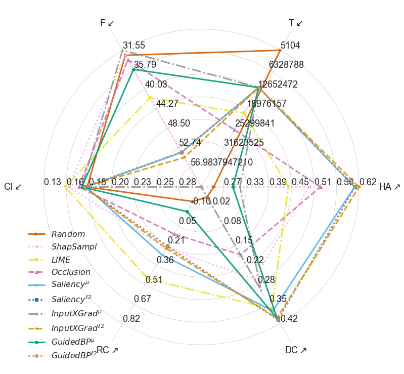
(a) $\mathtt{Transformer}$

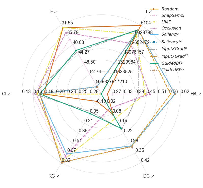
(b) $\mathtt{CNN}$

(c) $\mathtt{LSTM}$

Figure 2: Diagnostic property evaluation for all explainability techniques, on the e-SNLI dataset. The $\nearrow$ and $\swarrow$ signs indicate that higher, correpspondingly lower, values of the property measure are better.

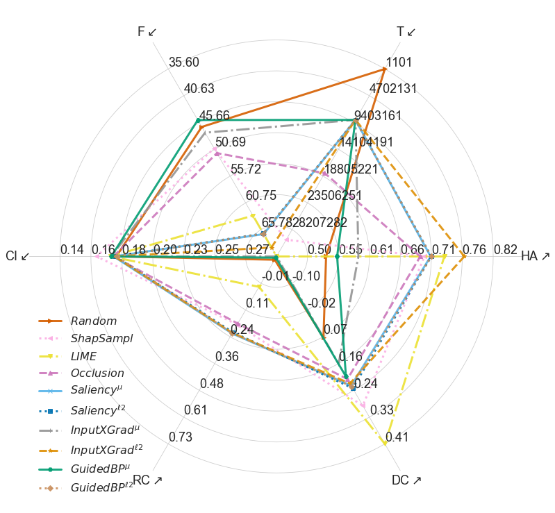
(a) $\mathtt{Transformer}$

(b) $\mathtt{CNN}$

(c) $\mathtt{LSTM}$

Figure 3: Diagnostic property evaluation for all explainability techniques, on the TSE dataset. The $\nearrow$ and $\swarrow$ signs indicate that higher, correspondingly lower, values of the property measure are better.

Diagnostic property performance. Figure 2 shows the performance of each explainability technique for all diagnostic properties on the e-SNLI dataset, and Figure 3 – for the TSE dataset, which are considerably bigger than IMDB. The IMDB dataset shows similar tendencies and a corresponding figure can be found in the supplementary material.

Agreement with human rationales. We observe that the best performing explainability technique for the $\mathtt{Transformer}$ model is $\textit{InputXGrad}^{\ell 2}$ followed by the gradient-based ones with L2 norm aggregation. While for the $\mathtt{CNN}$ and the $\mathtt{LSTM}$ models, we observe similar trends, their MAP scores are always lower than for the $\mathtt{Transformer}$, which indicates a correlation between the performance of a model and its agreement with human rationales. Furthermore, the MAP scores of the $\mathtt{CNN}$ model are higher than for the $\mathtt{LSTM}$ model, even though the latter achieves higher F1 scores on the e-SNLI dataset. This might indicate that the representations of the $\mathtt{LSTM}$ model are less in line with human rationales. Finally, we note that the mean aggregations of the gradient-based explainability techniques have MAP scores close to or even worse than those from the randomly initialized models.

Faithfulness. We find that gradient-based techniques have the best performance for the Faithfulness diagnostic property. On the e-SNLI dataset, it is particularly $\textit{InputXGrad}^{\ell 2}$, which performs well across all model architectures. We further find that the $\mathtt{CNN}$ exhibits the highest Faithfulness scores for seven out of nine explainability methods. We hypothesize that this is due to the simple architecture with relatively few neural nodes compared to the recurrent nature of the $\mathtt{LSTM}$ model and the large number of neural nodes in the $\mathtt{Transformer}$ architecture. Finally, models with high Faithfulness scores do not necessarily have high Human agreement scores and vice versa. This suggests that these two are indeed separate diagnostic properties, and the first should not be confused with estimating the faithfulness of the techniques.

Confidence Indication. We find that the Confidence Indication of all models is predicted most accurately by the ShapSampl, LIME, and Occlusion explainability methods. This result is expected, as they compute the saliency of words based on differences in the model’s confidence using different instance perturbations. We further find that the $\mathtt{CNN}$ model’s confidence is better predicted with $\textit{InputXGrad}^{\mu}$. The lowest MAE with the balanced dataset is for the $\mathtt{CNN}$ and $\mathtt{LSTM}$ models. We hypothesize that this could be due to these models’ overconfidence, which makes it challenging to detect when the model is not confident of its prediction.

Rationale Consistency. There is no single universal explainability technique that achieves the highest score for Rationale Consistency property. We see that LIME can be good at achieving a high performance, which is expected, as it is trained to approximate the model’s performance. The latter is beneficial, especially for models with complex architectures like the $\mathtt{Transformer}$. The gradient-based approaches also have high Rationale Consistency scores. We find that the Occlusion technique is the best performing for the $\mathtt{LSTM}$ across all tasks, as it is the simplest of the explored explainability techniques, and does not inspect the model’s internals or try to approximate them. This might serve as an indication that $\mathtt{LSTM}$ models, due to their recurrent nature, can be best explained with simple perturbation based methods that do not examine a model’s reasoning process.

Dataset Consistency. Finally, the results for the Dataset Consistency property show low to moderate correlations of the explainability techniques with similarities across instances in the dataset. The correlation is present for LIME and the gradient-based techniques, again with higher scores for the L2 aggregated gradient-based methods.

Overall. To summarise, the proposed list of diagnostic properties allows for assessing existing explainability techniques from different perspectives and supports the choice of the best performing one. Individual property results indicate that gradient-based methods have the best performance. The only strong exception to the above is the better performance of ShapSampl and LIME for the Confidence Indication diagnostic property. However, ShapSampl, LIME and Occlusion take considerably more time to compute and have worse performance for all other diagnostic properties.

6 Conclusion

We proposed a comprehensive list of diagnostic properties for the evaluation of explainability techniques from different perspectives. We further used them to compare and contrast different groups of explainability techniques on three downstream tasks and three diverse architectures. We found that gradient-based explanations are the best for all of the three models and all of the three downstream text classification tasks that we consider in this work. Other explainability techniques, such as ShapSampl, LIME and Occlusion take more time to compute, and are in addition considerably less faithful to the models and less consistent with the rationales of the models and similarities in the datasets.

Appendix A Appendices

A.1 Experimental Setup

Model	Time	Score
e-SNLI
$\mathtt{Transformer}$	244.763 ($\pm$62.022)	0.523 ($\pm$0.356)
$\mathtt{CNN}$	195.041 ($\pm$53.994)	0.756 ($\pm$0.028)
$\mathtt{LSTM}$	377.180 ($\pm$232.918)	0.708 ($\pm$0.205)
Movie Reviews
$\mathtt{Transformer}$	3.603 ($\pm$0.031)	0.785 ($\pm$0.226)
$\mathtt{CNN}$	4.777 ($\pm$1.953)	0.756 ($\pm$0.058)
$\mathtt{LSTM}$	5.344 ($\pm$1.593)	0.584 ($\pm$0.061)
TSE
$\mathtt{Transformer}$	9.393 ($\pm$1.841)	0.783 ($\pm$0.006)
$\mathtt{CNN}$	2.240 ($\pm$0.544)	0.730 ($\pm$0.035)
$\mathtt{LSTM}$	3.781 ($\pm$1.196)	0.713 ($\pm$0.076)

Table 4: Hyper-parameter tuning details. Time is the average time (mean and standard deviation in brackets) measured in minutes required for a particular model with all hyper-parameter combinations. Score is the mean and standard deviation of the performance on the validation set as a function of the number of the different hyper-parameter searches.

Machine Learning Models

. The models used in our experiments are trained on the training splits, and the parameters are selected according to the development split. We conducted fine-tuning in a grid-search manner with the ranges and parameters we describe next. We use superscripts to indicate when a parameter value was selected for one of the datasets e-SNLI – 1, Movie Review – 2, and TSE – 3. For the $\mathtt{CNN}$ model, we experimented with the following parameters: embedding dimension $\in\{50,100,200,300^{1,2,3}\}$, batch size $\in\{16^{2},32,64^{3},128,256^{1}\}$, dropout rate $\in\{0.05^{1,2,3},0.1,0.15,0.2\}$, learning rate for an Adam optimizer $\in\{0.01,0.03,0.001^{2,3},0.003,0.0001^{1},0.0003\}$, window sizes $\in\{[2,3,4]^{2},[2,3,4,5],[3,4,5]^{3},[3,4,5,6],$ $[4,5,6],[4,5,6,7]^{1}\}$, and number of output channels $\in\{50^{2,3},100,200,300^{1}\}$. We leave the stride and the padding parameters to their default values – one and zero.

For the $\mathtt{LSTM}$ model we fine-tuned over the following grid of parameters: embedding dimension $\in\{50^{3},100^{1,2},200,300\}$, batch size $\in\{16^{3},32,64,128^{2},256^{1}\}$, dropout rate $\in\{0.05^{3},0.1^{1,2},0.15,0.2\}$, learning rate for an Adam optimizer $\in\{0.01^{1},0.03^{2},0.001^{2,3},0.003,0.0001,0.0003\}$, number of LSTM layers $\in\{1^{2,3},2,3,4^{1}\}$, LSTM hidden layer size $\in\{50.100^{1,2,3},200,300\}$, and size of the two linear layers $\in\{[50,25]^{2},[100,50]^{1},[200,100]^{3}\}$. We also experimented with other numbers of linear layers after the recurrent ones, but having three of them, where the final was the prediction layer, yielded the best results.

The $\mathtt{CNN}$ and $\mathtt{LSTM}$ models are trained with an early stopping over the validation accuracy with a patience of five and a maximum number of training epochs of 100. We also experimented with other optimizers, but none yielded improvements.

Finally, for the $\mathtt{Transformer}$ model we fine-tuned the pre-trained basic, uncased LM Wolf et al. (2019)(110M parameters) where the maximum input size is 512, and the hidden size of each layer of the 12 layers is 768. We performed a grid-search over learning rate of $\in\{1e-5,2e-5^{1,2},3e-5^{3},4e-5,5e-5\}$. The models were trained with a warm-up period where the learning rate increases linearly between 0 and 1 for 0.05% of the steps found with a grid-search. We train the models for five epochs with an early stopping with patience of one as the Transformer models are easily fine-tuned for a small number of epochs.

All experiments were run on a single NVIDIA TitanX GPU with 8GB, and 4GB of RAM and 4 Intel Xeon Silver 4110 CPUs.

The models were evaluated with macro F1 score, which can be found here https://scikit-learn.org/stable/modules/generated/sklearn.metrics.precision_recall_fscore_support.html and is defined as follows:

$$Precision(P)=\frac{\mathrm{TP}}{\mathrm{TP}+\mathrm{FP}}$$

$$Recall(R)=\frac{\mathrm{TP}}{\mathrm{TP}+\mathrm{FN}}$$

$$F1=\frac{2*\mathrm{P}*\mathrm{R}}{\mathrm{P}+\mathrm{R}}$$

where TP is the number of true positives, FP is the number of false positives, and FN is the number of false negatives.

Explainability generation. When evaluating the Confidence Indication property of the explainability measures, we train a logistic regression for 5 splits and provide the MAE over the five test splits. As for some of the models, e.g. $\mathtt{Transformer}$, the confidence is always very high, the LR starts to predict only the average confidence. To avoid this, we additionally randomly up-sample the training instances with a smaller confidence, making the number of instances in each confidence interval [0.0-0.1],…[0.9-1.0]) to be the same as the maximum number of instances found in one of the separate intervals.

For both Rationale and Dataset Consistency properties, we consider Spearman’s $\rho$. While Pearson’s $\rho$ measures only the linear correlation between two variables (a change in one variable should be proportional to the change in the other variable), Spearman’s $\rho$ measures the monotonic correlation (when one variable increases, the other increases, too). In our experiments, we are interested in the monotonic correlation as all activation differences don’t have to be linearly proportional to the differences of the explanations and therefore measure Spearman’s $\rho$.

The Dataset Consistency property is estimated over instance pairs from the test dataset. As computing it for all possible pairs in the dataset is computationally expensive, we select 2 000 pairs from each dataset in order of their decreasing word overlap and sample 2 000 from the remaining instance pairs. This ensures that we compute the diagnostic property on a set containing tuples of similar and different instances.

Both the Dataset Consistency property and the Rationale Consistency property estimate the difference between the instances based on their activations. For the $\mathtt{LSTM}$ model, the activations of the LSTM layers are limited to the output activation also used for prediction as it isn’t possible to compare activations with different lengths due to the different token lengths of the different instances. We also use min-max scaling of the differences in the activations and the saliencies as the saliency scores assigned by some explainability techniques are very small.

A.2 Spider Figure for the IMDB dataset

(a) $\mathtt{Transformer}$

(b) $\mathtt{CNN}$

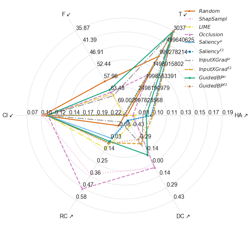
(c) $\mathtt{LSTM}$

Figure 4: Diagnostic property evaluation for all explainability techniques, on the IMDB dataset. The $\nearrow$ and $\swarrow$ signs following the names of each explainability method indicate that higher, correspondingly lower, values of the property measure are better.

A.3 Detailed explainability techniques evaluation results.

Explain.	e-SNLI			IMDB			TSE
	MAP	MAP RI	FLOPs	MAP	MAP RI	FLOPs	MAP	MAP RI	FLOPs
Random	.297 ($\pm$.001)	–	6.12e+3 ($\pm$4.6e+1)	.079 ($\pm$.001)	–	9.41e+4 ($\pm$1.8e+2)	.573 ($\pm$.001)	–	4.62e+3 ($\pm$2.2e+1)
$\mathtt{Transformer}$
ShapSampl	.511 ($\pm$.004)	.292 ($\pm$.011)	1.78e+7 ($\pm$5.5e+5)	.168 ($\pm$.003)	.084 ($\pm$.001)	3.00e+9 ($\pm$1.3e+8)	.716 ($\pm$.003)	.575 ($\pm$.027)	1.29e+7 ($\pm$2.0e+6)
LIME	.465 ($\pm$.008)	.264 ($\pm$.004)	2.39e+5 ($\pm$1.5e+4)	.127 ($\pm$.004)	.075 ($\pm$.004)	4.98e+8 ($\pm$1.4e+8)	.745 ($\pm$.003)	.570 ($\pm$.028)	2.82e+7 ($\pm$1.6e+6)
Occlusion	.537 ($\pm$.014)	.292 ($\pm$.009)	6.33e+5 ($\pm$1.0e+3)	.091 ($\pm$.001)	.084 ($\pm$.001)	8.05e+7 ($\pm$4.5e+5)	.710 ($\pm$.008)	.577 ($\pm$.012)	5.86e+5 ($\pm$1.6e+2)
$\textit{Saliency}^{\mu}$	.614 ($\pm$.003)	.255 ($\pm$.008)	5.38e+4 ($\pm$1.8e+2)	.187 ($\pm$.005)	.079 ($\pm$.001)	6.59e+5 ($\pm$1.8e+3)	.725 ($\pm$.011)	.499 ($\pm$.002)	4.93e+4 ($\pm$2.1e+2)
$\textit{Saliency}^{\ell 2}$	.615 ($\pm$.003)	.255 ($\pm$.009)	5.39e+4 ($\pm$1.3e+2)	.188 ($\pm$.006)	.078 ($\pm$.001)	6.62e+5 ($\pm$8.4e+2)	.726 ($\pm$.014)	.498 ($\pm$.001)	4.93e+4 ($\pm$1.4e+2)
$\textit{InputXGrad}^{\mu}$	.356 ($\pm$.005)	.280 ($\pm$.016)	5.38e+4 ($\pm$1.8e+2)	.118 ($\pm$.003)	.083 ($\pm$.001)	6.60e+5 ($\pm$4.5e+3)	.620 ($\pm$.008)	.558 ($\pm$.011)	4.92e+4 ($\pm$1.4e+2)
$\textit{InputXGrad}^{\ell 2}$	.624 ($\boldsymbol{\pm}$.004)	.254 ($\pm$.013)	5.39e+4 ($\pm$1.5e+2)	.193 ($\boldsymbol{\pm}$.005)	.079 ($\pm$.001)	6.62e+5 ($\pm$2.1e+3)	.774 ($\boldsymbol{\pm}$.009)	.499 ($\pm$.005)	4.92e+4 ($\pm$8.0e+1)
$\textit{GuidedBP}^{\mu}$	.340 ($\pm$.012)	.281 ($\pm$.025)	5.39e+4 ($\pm$1.8e+2)	.109 ($\pm$.003)	.086 ($\pm$.005)	6.54e+5 ($\pm$7.5e+3)	.589 ($\pm$.006)	.567 ($\pm$.008)	4.94e+4 ($\pm$4.1e+2)
$\textit{GuidedBP}^{\ell 2}$	.615 ($\pm$.003)	.255 ($\pm$.009)	5.38e+4 ($\pm$1.1e+2)	.189 ($\pm$.005)	.079 ($\pm$.001)	6.59e+5 ($\pm$2.8e+3)	.726 ($\pm$.012)	.498 ($\pm$.001)	4.97e+4 ($\pm$4.2e+2)
$\mathtt{CNN}$
ShapSampl	.471 ($\pm$.003)	.298 ($\pm$.008)	3.79e+7 ($\pm$3.1e+3)	.119 ($\pm$.004)	.084 ($\pm$.001)	1.26e+7 ($\pm$1.6e+5)	.789 ($\pm$.004)	.586 ($\pm$.017)	4.53e+6 ($\pm$2.1e+4)
LIME	.466 ($\pm$.002)	.300 ($\pm$.017)	1.81e+4 ($\pm$1.2e+3)	.125 ($\boldsymbol{\pm}$.005)	.079 ($\pm$.004)	5.39e+7 ($\pm$1.9e+4)	.737 ($\pm$.002)	.581 ($\pm$.021)	1.52e+4 ($\pm$7.1e+1)
Occlusion	.487 ($\pm$.003)	.298 ($\pm$.006)	6.06e+4 ($\pm$2.9e+2)	.090 ($\pm$.001)	.084 ($\pm$.001)	3.36e+5 ($\pm$2.6e+3)	.760 ($\pm$.004)	.580 ($\pm$.006)	1.40e+4 ($\pm$3.6e+1)
$\textit{Saliency}^{\mu}$	.600 ($\boldsymbol{\pm}$.002)	.339 ($\pm$.007)	1.08e+4 ($\pm$5.6e+1)	.114 ($\pm$.005)	.091 ($\pm$.001)	4.28e+3 ($\pm$2.3e+2)	.816 ($\pm$.003)	.593 ($\pm$.008)	4.16e+3 ($\pm$1.9e+1)
$\textit{Saliency}^{\ell 2}$	.600 ($\boldsymbol{\pm}$.002)	.339 ($\pm$.007)	1.06e+4 ($\pm$5.6e+1)	.115 ($\pm$.005)	.090 ($\pm$.001)	4.29e+3 ($\pm$9.9e+1)	.815 ($\pm$.003)	.596 ($\pm$.009)	4.16e+3 ($\pm$1.2e+1)
$\textit{InputXGrad}^{\mu}$	.435 ($\pm$.001)	.294 ($\pm$.014)	1.07e+4 ($\pm$2.3e+1)	.121 ($\pm$.003)	.086 ($\pm$.002)	4.27e+3 ($\pm$1.8e+2)	.736 ($\pm$.002)	.572 ($\pm$.011)	4.16e+3 ($\pm$1.2e+1)
$\textit{InputXGrad}^{\ell 2}$	.580 ($\pm$.001)	.280 ($\pm$.003)	1.06e+4 ($\pm$6.5e+1)	.113 ($\pm$.004)	.093 ($\pm$.002)	4.09e+3 ($\pm$1.8e+2)	.774 ($\pm$.003)	.501 ($\pm$.006)	4.12e+3 ($\pm$2.7e+1)
$\textit{GuidedBP}^{\mu}$	.269 ($\pm$.001)	.299 ($\pm$.017)	1.08e+4 ($\pm$1.7e+2)	.076 ($\pm$.002)	.086 ($\pm$.002)	4.27e+3 ($\pm$2.2e+2)	.501 ($\pm$.006)	.573 ($\pm$.013)	4.32e+3 ($\pm$4.0e+2)
$\textit{GuidedBP}^{\ell 2}$	.600 ($\boldsymbol{\pm}$.002)	.339 ($\pm$.007)	1.07e+4 ($\pm$3.4e+1)	.114 ($\pm$.005)	.091 ($\pm$.002)	4.21e+3 ($\pm$2.2e+2)	.815 ($\pm$.003)	.594 ($\pm$.009)	4.14e+3 ($\pm$1.7e+1)
$\mathtt{LSTM}$
ShapSampl	.396 ($\pm$.012)	.291 ($\pm$.008)	8.42e+5 ($\pm$1.2e+4)	.086 ($\pm$.001)	.084 ($\pm$.000)	2.30e+8 ($\pm$2.5e+5)	.605 ($\pm$.034)	.588 ($\pm$.020)	1.12e+7 ($\pm$2.1e+6)
LIME	.429 ($\pm$.012)	.309 ($\pm$.018)	1.68e+5 ($\pm$2.1e+5)	.089 ($\pm$.001)	.081 ($\pm$.002)	3.00e+8 ($\pm$1.8e+5)	.638 ($\pm$.025)	.588 ($\pm$.021)	5.20e+4 ($\pm$4.1e+3)
Occlusion	.358 ($\pm$.003)	.281 ($\pm$.007)	2.46e+5 ($\pm$5.7e+0)	.086 ($\pm$.002)	.083 ($\pm$.002)	1.18e+6 ($\pm$1.1e+3)	.694 ($\pm$.011)	.578 ($\pm$.016)	3.71e+4 ($\pm$2.7e+0)
$\textit{Saliency}^{\mu}$	.502 ($\pm$.008)	.411 ($\pm$.011)	5.11e+3 ($\pm$6.8e+0)	.108 ($\pm$.001)	.106 ($\pm$.000)	3.04e+3 ($\pm$7.7e+1)	.710 ($\pm$.009)	.546 ($\pm$.000)	1.11e+3 ($\pm$2.8e+0)
$\textit{Saliency}^{\ell 2}$	.502 ($\pm$.008)	.410 ($\pm$.010)	5.12e+3 ($\pm$4.6e+0)	.108 ($\pm$.002)	.106 ($\pm$.002)	3.07e+3 ($\pm$3.9e+1)	.710 ($\pm$.010)	.546 ($\pm$.001)	1.10e+3 ($\pm$1.4e+0)
$\textit{InputXGrad}^{\mu}$	.364 ($\pm$.004)	.349 ($\pm$.027)	5.12e+3 ($\pm$7.2e+0)	.098 ($\pm$.002)	.096 ($\pm$.002)	3.06e+3 ($\pm$7.0e+1)	.570 ($\pm$.010)	.601 ($\pm$.017)	1.11e+3 ($\pm$2.2e+0)
$\textit{InputXGrad}^{\ell 2}$	.511 ($\pm$.007)	.389 ($\pm$.004)	5.12e+3 ($\pm$4.2e+0)	.110 ($\boldsymbol{\pm}$.001)	.107 ($\pm$.000)	3.05e+3 ($\pm$9.9e+1)	.697 ($\pm$.007)	.544 ($\pm$.001)	1.10e+3 ($\pm$1.6e+0)
$\textit{GuidedBP}^{\mu}$	.333 ($\pm$.009)	.382 ($\pm$.033)	5.11e+3 ($\pm$4.4e+0)	.102 ($\pm$.005)	.098 ($\pm$.003)	3.06e+3 ($\pm$1.0e+2)	.527 ($\pm$.005)	.570 ($\pm$.031)	1.10e+3 ($\pm$2.2e+0)
$\textit{GuidedBP}^{\ell 2}$	.502 ($\pm$.009)	.410 ($\pm$.009)	5.10e+3 ($\pm$2.5e+1)	.109 ($\pm$.001)	.107 ($\pm$.001)	3.08e+3 ($\pm$9.2e+1)	.711 ($\boldsymbol{\pm}$.009)	.547 ($\pm$.001)	1.10e+3 ($\pm$2.4e+0)

Table 5: Evaluation of the explainability techniques with Human Agreement (HA) and time for computation. HA is measured with Mean Average Precision (MAP) with the gold human annotations, MAP of a Randomly initialized model (MAP RI). The time is computed with FLOPs. The presented numbers are averaged over five different models and the standard deviation of the scores is presented in brackets. Explainability methods with the best MAP for a particular dataset and model are in bold, while the best MAP across all models for a dataset is underlined as well. Methods that have MAP worse than the randomly generated saliency are in red.

Explain.	e-SNLI	IMDB	TSE
Random	56.05 ($\pm$0.71)	49.26 ($\pm$1.94)	56.45 ($\pm$2.37)
$\mathtt{Transformer}$
ShapSampl	56.05 ($\pm$0.71)	65.84 ($\pm$11.8)	52.99 ($\pm$4.24)
LIME	48.14 ($\pm$10.8)	59.04 ($\pm$13.7)	42.17 ($\pm$7.89)
Occlusion	55.24 ($\pm$3.77)	69.00 ($\pm$6.22)	52.23 ($\pm$4.29)
$\textit{Saliency}^{\mu}$	37.98 ($\pm$2.18)	49.32 ($\pm$9.01)	39.20 ($\boldsymbol{\pm}$3.06)
$\textit{Saliency}^{\ell 2}$	38.01 ($\pm$2.19)	49.05 ($\boldsymbol{\pm}$9.16)	39.29 ($\pm$3.14)
$\textit{InputXGrad}^{\mu}$	56.98 ($\pm$1.89)	64.47 ($\pm$8.70)	55.52 ($\pm$2.59)
$\textit{InputXGrad}^{\ell 2}$	37.05 ($\boldsymbol{\pm}$2.29)	50.22 ($\pm$8.85)	37.04 ($\pm$2.69)
$\textit{GuidedBP}^{\mu}$	53.43 ($\pm$1.00)	67.68 ($\pm$6.94)	57.56 ($\pm$2.60)
$\textit{GuidedBP}^{\ell 2}$	38.01 ($\pm$2.19)	49.47 ($\pm$8.89)	39.26 ($\pm$3.18)
$\mathtt{CNN}$
ShapSampl	51.78 ($\pm$2.24)	59.69 ($\pm$8.37)	64.72 ($\pm$1.75)
LIME	56.16 ($\pm$1.67)	59.09 ($\pm$8.48)	65.78 ($\pm$1.59)
Occlusion	54.32 ($\pm$0.94)	59.86 ($\pm$7.78)	61.17 ($\pm$1.48)
$\textit{Saliency}^{\mu}$	34.26 ($\pm$1.78)	49.61 ($\pm$5.26)	35.70 ($\pm$2.94)
$\textit{Saliency}^{\ell 2}$	34.16 ($\pm$1.81)	49.04 ($\boldsymbol{\pm}$5.60)	35.67 ($\pm$2.91)
$\textit{InputXGrad}^{\mu}$	47.06 ($\pm$3.82)	62.05 ($\pm$7.54)	64.45 ($\pm$2.99)
$\textit{InputXGrad}^{\ell 2}$	31.55 ($\boldsymbol{\pm}$2.83)	49.20 ($\pm$5.96)	35.86 ($\pm$3.22)
$\textit{GuidedBP}^{\mu}$	47.68 ($\pm$2.65)	67.03 ($\pm$4.36)	44.93 ($\pm$1.57)
$\textit{GuidedBP}^{\ell 2}$	34.16 ($\pm$1.81)	49.80 ($\pm$5.99)	35.60 ($\boldsymbol{\pm}$2.91)
$\mathtt{LSTM}$
ShapSampl	51.05 ($\pm$4.47)	44.05 ($\pm$3.06)	53.97 ($\pm$6.00)
LIME	51.93 ($\pm$7.73)	44.41 ($\pm$3.04)	54.95 ($\pm$3.19)
Occlusion	54.73 ($\pm$3.12)	45.01 ($\pm$3.84)	48.68 ($\pm$2.28)
$\textit{Saliency}^{\mu}$	38.29 ($\pm$1.77)	35.98 ($\pm$2.11)	37.20 ($\boldsymbol{\pm}$3.48)
$\textit{Saliency}^{\ell 2}$	38.26 ($\pm$1.84)	36.22 ($\pm$2.04)	37.23 ($\pm$3.50)
$\textit{InputXGrad}^{\mu}$	49.52 ($\pm$1.81)	43.57 ($\pm$4.98)	48.71 ($\pm$3.23)
$\textit{InputXGrad}^{\ell 2}$	37.95 ($\boldsymbol{\pm}$2.06)	36.03 ($\pm$1.97)	36.75 ($\pm$3.35)
$\textit{GuidedBP}^{\mu}$	44.48 ($\pm$2.12)	46.00 ($\pm$3.20)	43.72 ($\pm$5.69)
$\textit{GuidedBP}^{\ell 2}$	38.17 ($\pm$1.80)	35.87 ($\boldsymbol{\pm}$1.99)	37.21 ($\pm$3.48)

Table 6: Faithfulness-AUC for thresholds $\in$ [0, 10, 20, …, 100]. Lower scores indicate the ability of the saliency approach to assign higher scores to words more responsible for the final prediction. The presented scores are averaged over the different random initializations and the standard deviation is shown in brackets. Explainability methods with the smallest AUC for a particular dataset and model are in bold, while the smallest AUC across all models for a dataset is underlined as well. Methods that have AUC worse than the randomly generated saliency are in red.

	e-SNLI				IMDB				TSE
Explain.	MAE	MAX	MAE-up	MAX-up	MAE	MAX	MAE-up	MAX-up	MAE	MAX	MAE-up	MAX-up
Random	.087 ($\pm$.004)	.527 ($\pm$.007)	.276 ($\pm$.005)	.377 ($\pm$.002)	.130 ($\pm$.007)	.286 ($\pm$.014)	.160 ($\pm$.003)	.251 ($\pm$.008)	.092 ($\pm$.009)	.466 ($\pm$.021)	.260 ($\pm$.017)	.428 ($\pm$.064)
$\mathtt{Transformer}$
ShapSampl	.071 ($\pm$.005)	.456 ($\pm$.037)	.158 ($\pm$.029)	.437 ($\pm$.046)	.071 ($\boldsymbol{\pm}$.008)	.238 ($\boldsymbol{\pm}$.036)	.120 ($\boldsymbol{\pm}$.033)	.213 ($\boldsymbol{\pm}$.035)	.073 ($\boldsymbol{\pm}$.012)	.408 ($\boldsymbol{\pm}$.043)	.169 ($\boldsymbol{\pm}$.052)	.415 ($\boldsymbol{\pm}$.030)
LIME	.068 ($\boldsymbol{\pm}$.002)	.368 ($\boldsymbol{\pm}$.151)	.136 ($\boldsymbol{\pm}$.028)	.395 ($\boldsymbol{\pm}$.128)	.077 ($\pm$.008)	.288 ($\pm$.024)	.184 ($\pm$.018)	.260 ($\pm$.021)	.084 ($\pm$.009)	.521 ($\pm$.072)	.232 ($\pm$.013)	.661 ($\pm$.225)
Occlusion	.074 ($\pm$.004)	.499 ($\pm$.020)	.224 ($\pm$.006)	.518 ($\pm$.048)	.085 ($\pm$.011)	.306 ($\pm$.015)	.196 ($\pm$.015)	.252 ($\pm$.011)	.085 ($\pm$.011)	.463 ($\pm$.035)	.247 ($\pm$.015)	.482 ($\pm$.091)
$\textit{Saliency}^{\mu}$	.078 ($\pm$.005)	.544 ($\pm$.014)	.269 ($\pm$.004)	.416 ($\pm$.043)	.083 ($\pm$.009)	.303 ($\pm$.008)	.197 ($\pm$.017)	.269 ($\pm$.023)	.085 ($\pm$.012)	.474 ($\pm$.021)	.248 ($\pm$.017)	.467 ($\pm$.091)
$\textit{Saliency}^{\ell 2}$	.078 ($\pm$.005)	.565 ($\pm$.051)	.259 ($\pm$.007)	.571 ($\pm$.095)	.083 ($\pm$.009)	.306 ($\pm$.017)	.195 ($\pm$.021)	.245($\pm$.004)	.085 ($\pm$.012)	.465 ($\pm$.021)	.255 ($\pm$.012)	.479 ($\pm$.074)
$\textit{InputXGrad}^{\mu}$	.079 ($\pm$.005)	.502 ($\pm$.015)	.242 ($\pm$.006)	.518 ($\pm$.031)	.084 ($\pm$.011)	.310 ($\pm$.011)	.198 ($\pm$.013)	.246 ($\pm$.008)	.085 ($\pm$.011)	.463 ($\pm$.015)	.237 ($\pm$.010)	.480 ($\pm$.071)
$\textit{InputXGrad}^{\ell 2}$	.078 ($\pm$.005)	.568 ($\pm$.057)	.258 ($\pm$.007)	.581 ($\pm$.096)	.083 ($\pm$.011)	.301 ($\pm$.014)	.193 ($\pm$.023)	.249 ($\pm$.016)	.086 ($\pm$.013)	.469 ($\pm$.022)	.252 ($\pm$.016)	.480 ($\pm$.087)
$\textit{GuidedBP}^{\mu}$	.080 ($\pm$.005)	.505 ($\pm$.016)	.242 ($\pm$.008)	.519 ($\pm$.037)	.084 ($\pm$.011)	.308 ($\pm$.009)	.196 ($\pm$.014)	.245 ($\pm$.014)	.085 ($\pm$.011)	.456 ($\pm$.014)	.237 ($\pm$.013)	.494 ($\pm$.069)
$\textit{GuidedBP}^{\ell 2}$	.078 ($\pm$.005)	.565 ($\pm$.051)	.258 ($\pm$.007)	.573 ($\pm$.095)	.080 ($\pm$.012)	.306 ($\pm$.009)	.192 ($\pm$.018)	.244 ($\pm$.008)	.086 ($\pm$.012)	.503 ($\pm$.053)	.261 ($\pm$.017)	.450 ($\pm$.081)
$\mathtt{CNN}$
ShapSampl	.103 ($\boldsymbol{\pm}$.001)	.439 ($\pm$.020)	.133 ($\boldsymbol{\pm}$.003)	.643 ($\pm$.032)	.077 ($\pm$.018)	.210 ($\pm$.041)	.085 ($\pm$.023)	.196 ($\pm$.026)	.093 ($\pm$.002)	.372 ($\boldsymbol{\pm}$.011)	.148 ($\pm$.004)	.479 ($\pm$.030)
LIME	.125 ($\pm$.003)	.498 ($\pm$.018)	.190 ($\pm$.006)	.494 ($\pm$.028)	.128 ($\pm$.006)	.289 ($\pm$.019)	.156 ($\pm$.003)	.260 ($\pm$.011)	.103 ($\pm$.001)	.469 ($\pm$.027)	.202 ($\pm$.014)	.633 ($\pm$.090)
Occlusion	.119 ($\pm$.004)	.492 ($\pm$.018)	.176 ($\pm$.007)	.507 ($\pm$.037)	.130 ($\pm$.007)	.289 ($\pm$.018)	.160 ($\pm$.006)	.254 ($\pm$.005)	.114 ($\pm$.002)	.463 ($\pm$.018)	.250 ($\pm$.007)	.418 ($\pm$.035)
$\textit{Saliency}^{\mu}$	.137 ($\pm$.002)	.496 ($\pm$.011)	.220 ($\pm$.006)	.399 ($\pm$.010)	.129 ($\pm$.007)	.288 ($\pm$.021)	.159 ($\pm$.003)	.253 ($\pm$.013)	.115 ($\pm$.002)	.467 ($\pm$.014)	.245 ($\pm$.007)	.425 ($\pm$.028)
$\textit{Saliency}^{\ell 2}$	.140 ($\pm$.003)	.492 ($\pm$.009)	.225 ($\pm$.005)	.354 ($\boldsymbol{\pm}$.009)	.130 ($\pm$.006)	.286 ($\pm$.019)	.161 ($\pm$.004)	.250 ($\pm$.005)	.114 ($\pm$.002)	.475 ($\pm$.016)	.248 ($\pm$.006)	.405 ($\pm$.031)
$\textit{InputXGrad}^{\mu}$	.110 ($\pm$.001)	.436 ($\boldsymbol{\pm}$.014)	.153 ($\pm$.007)	.460 ($\pm$.009)	.071 ($\boldsymbol{\pm}$.004)	.191 ($\boldsymbol{\pm}$.010)	.071 ($\boldsymbol{\pm}$.005)	.190 ($\boldsymbol{\pm}$.010)	.090 ($\boldsymbol{\pm}$.002)	.379 ($\pm$.012)	.135 ($\boldsymbol{\pm}$.004)	.477 ($\boldsymbol{\pm}$.025)
$\textit{InputXGrad}^{\ell 2}$	.140 ($\pm$.003)	.492 ($\pm$.009)	.225 ($\pm$.005)	.355 ($\pm$.007)	.130 ($\pm$.007)	.285 ($\pm$.019)	.160 ($\pm$.004)	.251 ($\pm$.011)	.114 ($\pm$.002)	.475 ($\pm$.014)	.248 ($\pm$.006)	.416 ($\pm$.033)
$\textit{GuidedBP}^{\mu}$	.140 ($\pm$.003)	.485 ($\pm$.011)	.225 ($\pm$.005)	.367 ($\pm$.023)	.129 ($\pm$.006)	.286 ($\pm$.019)	.159 ($\pm$.003)	.253 ($\pm$.011)	.114 ($\pm$.002)	.462 ($\pm$.013)	.234 ($\pm$.011)	.441 ($\pm$.036)
$\textit{GuidedBP}^{\ell 2}$	.140 ($\pm$.003)	.492 ($\pm$.009)	.225 ($\pm$.005)	.353 ($\boldsymbol{\pm}$.008)	.130 ($\pm$.007)	.289 ($\pm$.018)	.159 ($\pm$.004)	.252 ($\pm$.011)	.114 ($\pm$.002)	.473 ($\pm$.015)	.249 ($\pm$.006)	.404 ($\boldsymbol{\pm}$.029)
$\mathtt{LSTM}$
ShapSampl	.118 ($\boldsymbol{\pm}$.003)	.622 ($\boldsymbol{\pm}$.035)	.131 ($\boldsymbol{\pm}$.005)	.648 ($\pm$.054)	.060 ($\boldsymbol{\pm}$.018)	.279 ($\boldsymbol{\pm}$.065)	.160 ($\boldsymbol{\pm}$.014)	.277 ($\pm$.038)	.087 ($\boldsymbol{\pm}$.007)	.433 ($\boldsymbol{\pm}$.053)	.147 ($\boldsymbol{\pm}$.015)	.393 ($\boldsymbol{\pm}$.029)
LIME	.127 ($\pm$.004)	.512 ($\pm$.052)	.145 ($\pm$.009)	.490 ($\pm$.040)	.069 ($\pm$.018)	.300 ($\pm$.051)	.209 ($\pm$.024)	.267 ($\pm$.031)	.090 ($\pm$.007)	.667 ($\pm$.150)	.218 ($\pm$.010)	.864 ($\pm$.362)
Occlusion	.147 ($\pm$.003)	.579 ($\pm$.065)	.172 ($\pm$.007)	.593 ($\pm$.083)	.069 ($\pm$.017)	.304 ($\pm$.055)	.216 ($\pm$.014)	.324 ($\pm$.032)	.099 ($\pm$.006)	.509 ($\pm$.015)	.259 ($\pm$.012)	.723 ($\pm$.063)
$\textit{Saliency}^{\mu}$	.163 ($\pm$.002)	.450 ($\pm$.008)	.195 ($\pm$.008)	.398 ($\pm$.031)	.069 ($\pm$.018)	.301 ($\pm$.051)	.208 ($\pm$.026)	.259 ($\boldsymbol{\pm}$.022)	.101 ($\pm$.007)	.518 ($\pm$.013)	.271 ($\pm$.008)	.469 ($\pm$.071)
$\textit{Saliency}^{\ell 2}$	.163 ($\pm$.002)	.448 ($\pm$.011)	.195 ($\pm$.008)	.399 ($\pm$.034)	.070 ($\pm$.018)	.299 ($\pm$.051)	.206 ($\pm$.024)	.263 ($\pm$.027)	.101 ($\pm$.007)	.523 ($\pm$.011)	.273 ($\pm$.008)	.441 ($\pm$.051)
$\textit{InputXGrad}^{\mu}$	.161 ($\pm$.002)	.454 ($\pm$.018)	.193 ($\pm$.007)	.502 ($\pm$.033)	.066 ($\pm$.018)	.295 ($\pm$.059)	.201 ($\pm$.033)	.262 ($\boldsymbol{\pm}$.014)	.098 ($\pm$.007)	.527 ($\pm$.005)	.268 ($\pm$.008)	.425 ($\pm$.035)
$\textit{InputXGrad}^{\ell 2}$	.163 ($\pm$.002)	.445 ($\boldsymbol{\pm}$.011)	.195 ($\pm$.007)	.394 ($\boldsymbol{\pm}$.029)	.068 ($\pm$.018)	.303 ($\pm$.050)	.201 ($\pm$.031)	.277 ($\pm$.024)	.101 ($\pm$.007)	.523 ($\pm$.008)	.273 ($\pm$.007)	.445 ($\pm$.038)
$\textit{GuidedBP}^{\mu}$	.161 ($\pm$.001)	.453 ($\pm$.014)	.192 ($\pm$.007)	.516 ($\pm$.058)	.068 ($\pm$.019)	.298 ($\pm$.055)	.200 ($\pm$.024)	.287 ($\pm$.045)	.097 ($\pm$.006)	.523 ($\pm$.017)	.260 ($\pm$.016)	.460 ($\pm$.045)
$\textit{GuidedBP}^{\ell 2}$	.163 ($\pm$.002)	.446 ($\pm$.010)	.195 ($\pm$.007)	.396 ($\pm$.042)	.069 ($\pm$.017)	.300 ($\pm$.050)	.204 ($\pm$.024)	.279 ($\pm$.025)	.101 ($\pm$.007)	.525 ($\pm$.010)	.273 ($\pm$.007)	.474 ($\pm$.051)

Table 7: Confidence Indication experiments are measured with the Mean Absolute Error (MAE) of the generated saliency scores when used to predict the confidence of the class predicted by the model and the Maximum Error (MAX). We present the result with and without up-sampling(MAE-up, MAX-up) of the model confidence. The presented measures are an average over the set of models trained from from different random seeds. The standard deviation of the scores is presented in brackets. AVG Conf. is the average confidence of the model for the predicted class. The best results for a particular dataset and model are in bold and the best results across a dataset are also underlined. Lower results are better.

Explain.	e-SNLI	IMDB	TSE
$\mathtt{Transformer}$
Random	-0.004 (2.6e-01)	-0.035 (1.4e-01)	0.003 (6.1e-01)
ShapSampl	0.310 (0.0e+00)	0.234 (3.6e-12)	0.259 (0.0e+00)
LIME	0.519 (0.0e+00)	0.269 (3.0e-31)	0.110 (2.0e-29)
Occlusion	0.215 (0.0e+00)	0.341 (2.6e-50)	0.255 (0.0e+00)
$\textit{Saliency}^{\mu}$	0.356 (0.0e+00)	0.423 (3.9e-79)	0.294 (0.0e+00)
$\textit{Saliency}^{\ell 2}$	0.297 (0.0e+00)	0.405 (6.9e-72)	0.289 (0.0e+00)
$\textit{InputXGrad}^{\mu}$	-0.102 (2.0e-202)	0.426 (2.5e-80)	-0.010 (1.3e-01)
$\textit{InputXGrad}^{\ell 2}$	0.311 (0.0e+00)	0.397 (3.8e-69)	0.292 (0.0e+00)
$\textit{GuidedBP}^{\mu}$	0.064 (1.0e-79)	-0.083 (4.2e-04)	-0.005 (4.9e-01)
$\textit{GuidedBP}^{\ell 2}$	0.297 (0.0e+00)	0.409 (1.2e-73)	0.293 (0.0e+00)
$\mathtt{CNN}$
Random	-0.003 (4.0e-01)	0.426 (2.6e-106)	-0.002 (7.4e-01)
ShapSampl	0.789 (0.0e+00)	0.537 (1.4e-179)	0.704 (0.0e+00)
LIME	0.790 (0.0e+00)	0.584 (1.9e-219)	0.730 (0.0e+00)
Occlusion	0.730 (0.0e+00)	0.528 (2.4e-172)	0.372 (0.0e+00)
$\textit{Saliency}^{\mu}$	0.701 (0.0e+00)	0.460 (4.5e-126)	0.320 (0.0e+00)
$\textit{Saliency}^{\ell 2}$	0.819 (0.0e+00)	0.583 (4.0e-218)	0.499 (0.0e+00)
$\textit{InputXGrad}^{\mu}$	0.136 (0.0e+00)	0.331 (1.2e-62)	0.002 (7.5e-01)
$\textit{InputXGrad}^{\ell 2}$	0.816 (0.0e+00)	0.585 (8.6e-221)	0.495 (0.0e+00)
$\textit{GuidedBP}^{\mu}$	0.160 (0.0e+00)	0.373 (5.5e-80)	0.173 (6.3e-121)
$\textit{GuidedBP}^{\ell 2}$	0.819 (0.0e+00)	0.578 (2.4e-214)	0.498 (0.0e+00)
$\mathtt{LSTM}$
Random	0.004 (1.8e-01)	0.002 (9.2e-01)	0.010 (1.8e-01)
ShapSampl	0.657 (0.0e+00)	0.382 (1.7e-63)	0.502 (0.0e-00)
LIME	0.700 (0.0e+00)	0.178 (3.3e-14)	0.540 (0.0e-00)
Occlusion	0.697 (0.0e+00)	0.498 (1.7e-113)	0.454 (0.0e-00)
$\textit{Saliency}^{\mu}$	0.645 (0.0e+00)	0.098 (3.1e-05)	0.667 (0.0e-00)
$\textit{Saliency}^{\ell 2}$	0.662 (0.0e+00)	0.132 (1.8e-08)	0.596 (0.0e-00)
$\textit{InputXGrad}^{\mu}$	0.026 (1.9e-14)	-0.032 (1.7e-01)	0.385 (0.0e-00)
$\textit{InputXGrad}^{\ell 2}$	0.664 (0.0e+00)	0.133 (1.5e-08)	0.604 (0.0e-00)
$\textit{GuidedBP}^{\mu}$	0.144 (0.0e+00)	0.122 (2.0e-07)	0.295 (0.0e-00)
$\textit{GuidedBP}^{\ell 2}$	0.663 (0.0e+00)	0.139 (3.1e-09)	0.598 (0.0e-00)

Table 8: Rationale Consistency Spearman’s $\rho$ correlation. The estimated p-value for the correlation is provided in the brackets. The best results for a particular dataset and model are in bold and the best results across a dataset are also underlined. Correlation lower that the one of the randomly sampled saliency scores are colored in red.

Explain.	e-SNLI	IMDB	TSE
$\mathtt{Transformer}$
Random	0.047 (2.7e-04)	0.127 (6.6e-07)/	0.121 (2.5e-01)
ShapSampl	0.285 (1.8e-02)	0.078 (5.8e-04)	0.308 (3.4e-36)
LIME	0.372 (3.1e-90)	0.236 (4.6e-07)	0.413 (3.4e-120)
Occlusion	0.215 (9.6e-02)	0.003 (2.0e-04)	0.235 (7.3e-05)
$\textit{Saliency}^{\mu}$	0.378 (4.3e-57)	0.023 (4.3e-02)	0.253 (1.4e-20)
$\textit{Saliency}^{\ell 2}$	0.027 (3.0e-05)	-0.043 (5.6e-02)	0.260 (6.8e-21)
$\textit{InputXGrad}^{\mu}$	0.319 (3.0e-03)	0.008 (1.2e-01)	0.193 (7.5e-05)
$\textit{InputXGrad}^{\ell 2}$	0.399 (1.9e-78)	0.028 (2.3e-03)	0.247 (4.9e-17)
$\textit{GuidedBP}^{\mu}$	0.400 (6.7e-31)	0.017 (1.9e-01)	0.228 (5.2e-09)
$\textit{GuidedBP}^{\ell 2}$	0.404 (1.4e-84)	0.019 (4.3e-04)	0.255 (3.1e-20)
$\mathtt{CNN}$
Random	0.018 (2.4e-01)	0.115 (1.8e-04)	0.008 (2.0e-01)
ShapSampl	0.015 (1.8e-01)	-0.428 (5.3e-153)	0.037 (1.4e-01)
LIME	0.000 (4.4e-02)	0.400 (1.4e-126)	0.023 (4.0e-01)
Occlusion	-0.076 (6.5e-02)	-0.357 (1.9e-85)	0.041 (1.7e-01)
$\textit{Saliency}^{\mu}$	0.381 (6.9e-91)	0.431 (1.1e-146)	-0.100 (3.9e-06)
$\textit{Saliency}^{\ell 2}$	0.391 (1.7e-98)	0.427 (3.5e-135)	-0.100 (3.7e-06)
$\textit{InputXGrad}^{\mu}$	0.171 (5.1e-04)	0.319 (1.4e-69)	0.024 (3.5e-01)
$\textit{InputXGrad}^{\ell 2}$	0.399 (1.0e-93)	0.428 (1.4e-132)	-0.076 (1.2e-03)
$\textit{GuidedBP}^{\mu}$	0.091 (7.9e-02)	0.375 (5.7e-109)	-0.032 (1.1e-01)
$\textit{GuidedBP}^{\ell 2}$	0.391 (1.7e-98)	0.432 (3.5e-140)	-0.102 (1.7e-06)
$\mathtt{LSTM}$
Random	0.018 (3.9e-01)	0.037 (1.8e-01)	0.016 (9.2e-03)
ShapSampl	0.398 (3.5e-81)	0.230 (8.9e-03)	0.205 (2.1e-16)
LIME	0.415 (1.2e-80)	0.079 (8.6e-04)	0.207 (4.3e-16)
Occlusion	0.363 (1.1e-37)	0.429 (7.5e-137)	0.237 (2.9e-29)
$\textit{Saliency}^{\mu}$	0.158 (1.7e-17)	-0.177 (1.6e-10)	0.065 (5.8e-03)
$\textit{Saliency}^{\ell 2}$	0.160 (7.5e-19)	-0.168 (2.0e-15)	0.096 (8.2e-03)
$\textit{InputXGrad}^{\mu}$	0.142 (3.3e-06)	-0.152 (1.2e-14)	0.106 (2.8e-02)
$\textit{InputXGrad}^{\ell 2}$	0.183 (7.0e-24)	-0.175 (4.7e-17)	0.089 (8.4e-03)
$\textit{GuidedBP}^{\mu}$	0.163 (1.9e-12)	-0.060 (4.7e-02)	0.077 (1.2e-02)
$\textit{GuidedBP}^{\ell 2}$	0.169 (1.8e-12)	-0.214 (5.8e-16)	0.115 (4.3e-02)

Table 9: Dataset Consistency results with Spearman $\rho$. The estimated p-value for the correlation is provided in the brackets. The best results for a particular dataset and model are in bold and the best results across a dataset are also underlined. Correlation lower that the one of the randomly samples saliency scores are colored in red.

References

- Adebayo et al. (2018) Julius Adebayo, Justin Gilmer, Michael Muelly, Ian Goodfellow, Moritz Hardt, and Been Kim. 2018. Sanity Checks for Saliency Maps. In Proceedings of the 32Nd International Conference on Neural Information Processing Systems, NIPS’18, pages 9525–9536, USA. Curran Associates Inc.
- Alvarez-Melis and Jaakkola (2018) David Alvarez-Melis and Tommi S Jaakkola. 2018. On the robustness of interpretability methods. arXiv preprint arXiv:1806.08049.
- Arras et al. (2019) Leila Arras, Ahmed Osman, Klaus-Robert Müller, and Wojciech Samek. 2019. Evaluating Recurrent Neural Network Explanations. In Proceedings of the 2019 ACL Workshop BlackboxNLP: Analyzing and Interpreting Neural Networks for NLP, pages 113–126, Florence, Italy. Association for Computational Linguistics.
- Arrieta et al. (2020) Alejandro Barredo Arrieta, Natalia Díaz-Rodríguez, Javier Del Ser, Adrien Bennetot, Siham Tabik, Alberto Barbado, Salvador Garcia, Sergio Gil-Lopez, Daniel Molina, Richard Benjamins, Raja Chatila, and Francisco Herrera. 2020. Explainable Artificial Intelligence (XAI): Concepts, taxonomies, opportunities and challenges toward responsible AI. Information Fusion, 58:82 – 115.
- Atanasova et al. (2020a) Pepa Atanasova, Jakob Grue Simonsen, Christina Lioma, and Isabelle Augenstein. 2020a. Generating Fact Checking Explanations. In ACL, pages 7352–7364. Association for Computational Linguistics.
- Atanasova et al. (2020b) Pepa Atanasova, Dustin Wright, and Isabelle Augenstein. 2020b. Generating Label Cohesive and Well-Formed Adversarial Claims. In Proceedings of EMNLP. Association for Computational Linguistics.
- Bansal et al. (2016) Trapit Bansal, David Belanger, and Andrew McCallum. 2016. Ask the GRU: Multi-Task Learning for Deep Text Recommendations. In Proceedings of the 10th ACM Conference on Recommender Systems, RecSys ’16, page 107–114, New York, NY, USA. Association for Computing Machinery.
- Camburu et al. (2018) Oana-Maria Camburu, Tim Rocktäschel, Thomas Lukasiewicz, and Phil Blunsom. 2018. e-SNLI: Natural Language Inference with Natural Language Explanations. In S. Bengio, H. Wallach, H. Larochelle, K. Grauman, N. Cesa-Bianchi, and R. Garnett, editors, Advances in Neural Information Processing Systems 31, pages 9539–9549. Curran Associates, Inc.
- Caruana et al. (2015) Rich Caruana, Yin Lou, Johannes Gehrke, Paul Koch, Marc Sturm, and Noemie Elhadad. 2015. Intelligible Models for HealthCare: Predicting Pneumonia Risk and Hospital 30-Day Readmission. In Proceedings of the 21th ACM SIGKDD International Conference on Knowledge Discovery and Data Mining, KDD ’15, page 1721–1730, New York, NY, USA. Association for Computing Machinery.
- Castro et al. (2009) Javier Castro, Daniel Gómez, and Juan Tejada. 2009. Polynomial Calculation of the Shapley Value Based on Sampling. Comput. Oper. Res., 36(5):1726–1730.
- Clark et al. (2019) Christopher Clark, Kenton Lee, Ming-Wei Chang, Tom Kwiatkowski, Michael Collins, and Kristina Toutanova. 2019. BoolQ: Exploring the Surprising Difficulty of Natural Yes/No Questions. In Proceedings of the 2019 Conference of the North American Chapter of the Association for Computational Linguistics: Human Language Technologies, Volume 1 (Long and Short Papers), pages 2924–2936, Minneapolis, Minnesota. Association for Computational Linguistics.
- Devlin et al. (2019) Jacob Devlin, Ming-Wei Chang, Kenton Lee, and Kristina Toutanova. 2019. BERT: Pre-training of Deep Bidirectional Transformers for Language Understanding. In Proceedings of the 2019 Conference of the North American Chapter of the Association for Computational Linguistics: Human Language Technologies, Volume 1 (Long and Short Papers), pages 4171–4186, Minneapolis, Minnesota. Association for Computational Linguistics.
- DeYoung et al. (2020) Jay DeYoung, Sarthak Jain, Nazneen Fatema Rajani, Eric Lehman, Caiming Xiong, Richard Socher, and Byron C Wallace. 2020. ERASER: A Benchmark to Evaluate Rationalized NLP Models. 2020.
- Feng et al. (2018) Shi Feng, Eric Wallace, Alvin Grissom II, Mohit Iyyer, Pedro Rodriguez, and Jordan Boyd-Graber. 2018. Pathologies of Neural Models Make Interpretations Difficult. In Proceedings of the 2018 Conference on Empirical Methods in Natural Language Processing, pages 3719–3728, Brussels, Belgium. Association for Computational Linguistics.
- Fukushima (1980) Kunihiko Fukushima. 1980. Neocognitron: A self-organizing neural network model for a mechanism of pattern recognition unaffected by shift in position. Biological cybernetics, 36(4):193–202.
- Guan et al. (2019) Chaoyu Guan, Xiting Wang, Quanshi Zhang, Runjin Chen, Di He, and Xing Xie. 2019. Towards a Deep and Unified Understanding of Deep Neural Models in NLP. In Proceedings of the 36th International Conference on Machine Learning, volume 97 of Proceedings of Machine Learning Research, pages 2454–2463, Long Beach, California, USA. PMLR.
- Hahnloser et al. (2000) Richard HR Hahnloser, Rahul Sarpeshkar, Misha A Mahowald, Rodney J Douglas, and H Sebastian Seung. 2000. Digital selection and analogue amplification coexist in a cortex-inspired silicon circuit. Nature, 405(6789):947–951.
- Hochreiter and Schmidhuber (1997) Sepp Hochreiter and Jürgen Schmidhuber. 1997. Long short-term memory. Neural computation, 9(8):1735–1780.
- Jacovi and Goldberg (2020) Alon Jacovi and Yoav Goldberg. 2020. Towards faithfully interpretable nlp systems: How should we define and evaluate faithfulness? arXiv preprint arXiv:2004.03685.
- Johansson et al. (2004) Ulf Johansson, Rikard König, and Lars Niklasson. 2004. The Truth is in There Rule Extraction from Opaque Models Using Genetic Programming. In Proceedings of the Seventeenth International Florida Artificial Intelligence Research Society Conference, FLAIRS 2004. AAAI Press.
- Khashabi et al. (2018) Daniel Khashabi, Snigdha Chaturvedi, Michael Roth, Shyam Upadhyay, and Dan Roth. 2018. Looking Beyond the Surface: A Challenge Set for Reading Comprehension over Multiple Sentences. In Proceedings of the 2018 Conference of the North American Chapter of the Association for Computational Linguistics: Human Language Technologies, Volume 1 (Long Papers), pages 252–262, New Orleans, Louisiana. Association for Computational Linguistics.
- Kindermans et al. (2019) Pieter-Jan Kindermans, Sara Hooker, Julius Adebayo, Maximilian Alber, Kristof T Schütt, Sven Dähne, Dumitru Erhan, and Been Kim. 2019. The (un) reliability of saliency methods. In Explainable AI: Interpreting, Explaining and Visualizing Deep Learning, pages 267–280. Springer.
- Kindermans et al. (2016) Pieter-Jan Kindermans, Kristof Schütt, Klaus-Robert Müller, and Sven Dähne. 2016. Investigating the influence of noise and distractors on the interpretation of neural networks. ArXiv, abs/1611.07270.
- Lei et al. (2016) Tao Lei, Regina Barzilay, and Tommi Jaakkola. 2016. Rationalizing Neural Predictions. In Proceedings of the 2016 Conference on Empirical Methods in Natural Language Processing, pages 107–117, Austin, Texas. Association for Computational Linguistics.
- Lertvittayakumjorn and Toni (2019) Piyawat Lertvittayakumjorn and Francesca Toni. 2019. Human-grounded Evaluations of Explanation Methods for Text Classification. In Proceedings of the 2019 Conference on Empirical Methods in Natural Language Processing and the 9th International Joint Conference on Natural Language Processing (EMNLP-IJCNLP), pages 5195–5205, Hong Kong, China. Association for Computational Linguistics.
- Lundberg and Lee (2017) Scott M Lundberg and Su-In Lee. 2017. A unified approach to interpreting model predictions. In Advances in neural information processing systems, pages 4765–4774.
- Martens et al. (2008) David Martens, Johan Huysmans, Rudy Setiono, Jan Vanthienen, and Bart Baesens. 2008. Rule Extraction from Support Vector Machines: An Overview of Issues and Application in Credit Scoring, pages 33–63. Springer Berlin Heidelberg, Berlin, Heidelberg.
- Narayanan et al. (2018) Menaka Narayanan, Emily Chen, Jeffrey He, Been Kim, Sam Gershman, and Finale Doshi-Velez. 2018. How do humans understand explanations from machine learning systems? an evaluation of the human-interpretability of explanation. arXiv preprint arXiv:1802.00682.
- Pennington et al. (2014) Jeffrey Pennington, Richard Socher, and Christopher D. Manning. 2014. GloVe: Global Vectors for Word Representation. In Empirical Methods in Natural Language Processing (EMNLP), pages 1532–1543.
- Poerner et al. (2018) Nina Poerner, Hinrich Schütze, and Benjamin Roth. 2018. Evaluating neural network explanation methods using hybrid documents and morphosyntactic agreement. In Proceedings of the 56th Annual Meeting of the Association for Computational Linguistics (Volume 1: Long Papers), pages 340–350, Melbourne, Australia. Association for Computational Linguistics.
- Regulation (2016) General Data Protection Regulation. 2016. Regulation (eu) 2016/679 of the european parliament and of the council of 27 april 2016 on the protection of natural persons with regard to the processing of personal data and on the free movement of such data, and repealing directive 95/46. Official Journal of the European Union (OJ), 59(1-88):294.
- Ribeiro et al. (2016) Marco Tulio Ribeiro, UW EDU, Sameer Singh, and Carlos Guestrin. 2016. Model-Agnostic Interpretability of Machine Learning. In ICML Workshop on Human Interpretability in Machine Learning.
- Rich (2016) Michael L Rich. 2016. Machine learning, automated suspicion algorithms, and the fourth amendment. University of Pennsylvania Law Review, pages 871–929.
- Robnik-Šikonja and Bohanec (2018) Marko Robnik-Šikonja and Marko Bohanec. 2018. Perturbation-based explanations of prediction models. In Human and machine learning, pages 159–175. Springer.
- Shapley (1953) Lloyd S Shapley. 1953. A value for n-person games. Contributions to the Theory of Games, 2(28):307–317.
- Simonyan et al. (2013) Karen Simonyan, Andrea Vedaldi, and Andrew Zisserman. 2013. Deep Inside Convolutional Networks: Visualising Image Classification Models and Saliency Maps. CoRR, abs/1312.6034.
- Springenberg et al. (2014) Jost Tobias Springenberg, Alexey Dosovitskiy, Thomas Brox, and Martin Riedmiller. 2014. Striving for simplicity: The all convolutional net. arXiv preprint arXiv:1412.6806.
- Subramanian et al. (2020) Sanjay Subramanian, Ben Bogin, Nitish Gupta, Tomer Wolfson, Sameer Singh, Jonathan Berant, and Matt Gardner. 2020. Obtaining faithful interpretations from compositional neural networks. arXiv preprint arXiv:2005.00724.
- Sundararajan et al. (2017) Mukund Sundararajan, Ankur Taly, and Qiqi Yan. 2017. Axiomatic attribution for deep networks. In Proceedings of the 34th International Conference on Machine Learning-Volume 70, pages 3319–3328. JMLR. org.
- Vashishth et al. (2019) Shikhar Vashishth, Shyam Upadhyay, Gaurav Singh Tomar, and Manaal Faruqui. 2019. Attention interpretability across nlp tasks. arXiv preprint arXiv:1909.11218.
- Vaswani et al. (2017) Ashish Vaswani, Noam Shazeer, Niki Parmar, Jakob Uszkoreit, Llion Jones, Aidan N Gomez, Łukasz Kaiser, and Illia Polosukhin. 2017. Attention is all you need. In Advances in neural information processing systems, pages 5998–6008.
- Wagner et al. (2019) Jörg Wagner, Jan Mathias Köhler, Tobias Gindele, Leon Hetzel, Jakob Thaddäus Wiedemer, and Sven Behnke. 2019. Interpretable and Fine-Grained Visual Explanations for Convolutional Neural Networks. In 2019 IEEE/CVF Conference on Computer Vision and Pattern Recognition (CVPR), pages 9089–9099. IEEE.
- Wolf et al. (2019) Thomas Wolf, Lysandre Debut, Victor Sanh, Julien Chaumond, Clement Delangue, Anthony Moi, Pierric Cistac, Tim Rault, R’emi Louf, Morgan Funtowicz, and Jamie Brew. 2019. HuggingFace’s Transformers: State-of-the-art Natural Language Processing. ArXiv, abs/1910.03771.
- Zaidan et al. (2007) Omar Zaidan, Jason Eisner, and Christine Piatko. 2007. Using “Annotator Rationales” to Improve Machine Learning for Text Categorization. In Human Language Technologies 2007: The Conference of the North American Chapter of the Association for Computational Linguistics; Proceedings of the Main Conference, pages 260–267, Rochester, New York. Association for Computational Linguistics.
- Zeiler and Fergus (2014) Matthew D Zeiler and Rob Fergus. 2014. Visualizing and understanding convolutional networks. In European conference on computer vision, pages 818–833. Springer.