Generalized Gravitational Baryogenesis of Well-Known $f(T,T_{G})$ and $f(T,B)$ Models

Abstract

The baryogenesis presents the theoretical mechanism that describes the matter-antimatter asymmetry in the history of early universe. In this work, we investigate the gravitational baryogenesis phenomena in the frameworks of $f(T,T_{G})$ (where $T$ and $T_{G}$ are the torsion scalar and teleparallel equivalent to the Gauss-Bonnet term respectively) and $f(T,B)$ (where $B$ denotes the boundary term between torsion and Ricci scalar) gravities. For $f(T,T_{G})$-gravity, we consider two generic power law models while logarithmic and general Taylor expansion models for $f(T,B)$-gravity. We consider power law scale factor for each model and compute baryon to entropy ratio by assuming that the universe filled by perfect fluid and dark energy. We find generalized baryogenesis interaction which is proportional to $\partial_{\mu}f(T+T_{G})$ and $\partial_{\mu}f(T+B)$ for both theories of gravity. We compare our results against current astrophysical data of baryon to entropy ratio, which indicates excellent consistency with observational bounds (i.e., $\frac{\eta_{B}}{S}=9.42\times 10^{-11}$).

Keywords: Baryogenesis; Baryon to entropy ratio; $f(T,T_{G})$-gravity; $f(T,B)$-gravity.

I Introduction

The excess of matter over antimatter remains not only a biggest puzzle in the history of early universe, but also an open problem in modern cosmology. The observational data like measurements of cosmic microwave background (CBM) 1 , supported with big bang nucleosynthesis 2 , indicate more matter than antimatter in the universe. Many authors presented a lot of theories to explore this enigma, some of which are Affleck-Dine baryogenesis 3 -5 , electroweak baryogenesis 6 ; 7 , grand unified theories (GUTs) 8 , spontaneous baryogenesis 9 -11 , baryogenesis of thermal and black hole evaporation 12 , all these theories explain why there exists matter antimatter asymmetry in our universe. Observational constrains verify that the baryon number density to entropy ratio is approximately $\frac{\eta_{B}}{S}\sim 9.42\times 10^{-11}$ 1 ; 2 where $\eta_{B}$ and $S$ denotes the number of baryon, and the entropy of universe, respectively. Sakharov 13 pointed out three fundamental conditions which are needed to generate baryon asymmetry. These conditions are

• processes that violate baryon number,

• violation of charge (C) and charge-parity (CP) symmetry,

• thermal inequilibrium.

Davoudiasl et al. 14 proposed required matter-antimatter asymmetry by the means of thermal equilibrium during transition phase of universe while CP dynamically violated. The key ingredient is a CP violating interaction which specified by coupling between between the baryon matter current $J^{\mu}$ and the derivative of the Ricci scalar curvature $R$, in the form

$$\frac{1}{M_{*}^{2}}\int{\sqrt{-g}d^{4}x(\partial_{\mu}R)J^{\mu}},$$ (1)

where $M_{*}$ characterizes the cutoff scale of the underlying effective gravitational theory 15 . In case of flat FRW geometry $\frac{\eta_{B}}{S}\propto\dot{R}$, where overhead dot means the derivative of $R$ with respect to time $t$. In case of radiation dominated era whose equation of state $w=\frac{1}{3}$, the net baryon asymmetry produced by Eq.(1) tends to be zero.

Many authors extended baryogenesis phenomena in the framework of modified theories gravity, which developed by modifying the Einstein Hilbert action. In these theories of gravity, curvature-based formulation of general relativity is the interesting and suitable modification. However, teleparallel equivalent to general relativity (TEGR) is another promising modification, in which curvature scalar replaced by torsional formulation. Gravitational framework of this theory, Lagrangian density support Weitzenböck connection instead of the torsion-less Levi-Civita. Further generalization form of this theory can be obtained by using general function $f(T)$ instead of torsion scalar $T$, namely $f(T)$-gravity. Hence, similarly to the $f(T)$-gravity, one can construct $f(R)$ as a extensions of TEGR by replacing curvature scalar $R$ instead of Lagrangian density. $f(T)$ and $f(R)$ represent different modification classes, therefore they do not coincide with each other.

Beside this simple modification, one can construct more complicated classes by introducing higher-torsion corrections just like Gauss-Bonnet (GB) term $G$ 15a , Weyl combinations 15b , Love-lock combinations 15c etc. Based on this concept, another modification of Einstein s theory presented known as $f(T_{G})$-gravity 15d . Hence by adding $f(T)$ term, another generalization of $f(T_{G})$-gravity presented known as $f(T,T_{G})$ gravity. Recently, a latest modification of $f(T)$-gravity was proposed by introducing a new Lagrangian $f(T,B)$, where $B$ is the boundary term related to the divergence of the torsion tensor ($B=2\nabla_{\mu}(T^{\mu})$). The $f(T,B)$-gravity 15e becomes equivalent to $f(R)$ for the special choice $f(-T+B)$.

Nojiri and Odintsov nl1 reviewed various modified theories of gravity and found that these theories have quite rich cosmological structure. These theories demonstrated effective late-time era (cosmological constant, quintessence or phantom) with a possible transition from deceleration to acceleration and may pass the solar system tests. Same authors nl2 discussed the general properties and different representations of string-inspired and Gauss-Bonnet theory, $f(R)$-gravity and its modified form, nonlocal gravity, scalar-tensor theory, power-counting renormalizable covariant gravity. Felice and Tsujikawa nl3 worked on dark energy, inflation, cosmological perturbations, local gravity constraints and spherically symmetric solutions in weak and strong gravitational backgrounds by consider $f(R)$-gravity. Various well known dark energy models for different fluids are explicitly realized, and their properties are also explored nl4 . They found these dark energy universes may mimic the $\Lambda$CDM model currently, consistent with the recent observational data also paid special attention to the equivalence of different dark energy models. Nojiri et al. new discussed some astrophysical solutions and their several qualitative features in the framework of modified theories of gravity. They emphasized on late-time acceleration of universe, inflation, bouncing cosmology and formed a virtual toolbox, which cover all necessary information about these cosmological terms. However, Oikonomou new1 investigated how the baryogenesis phenomena can potentially constrain the construction of a Type IV singularity. For loop quantum cosmology new2 authors discussed the cases under which constrains of baryon to entropy ratio well match with observations.

In the past few years, gravitational baryogenesis studied in various modified theories of gravity. Some authors 16 ; 17 studied baryogenesis phenomena in nonminimally coupled $f(R)$ theories and $f(R)$ gravity respectively. They found only for tiny deviations of a few percent, are consistent with the current bounds. In 18 , Odintsov and Oikonomou investigated the ratio of the baryon number to entropy density for the Gauss-Bonnet baryogenesis term while Oikonomou and Saridakis 19 discussed baryogenesis by considering different cases of $f(T)$-gravity. Bento et al. 22 investigated baryogenesis in the framework of GB braneworld cosmology, they also investigated the effect of the novel terms on the baryon-to-entropy ratio. This mechanism were further developed in minimal $f(R,\mathcal{T})$ gravity 20 (where $\mathcal{T}$ denotes the trace of stress energy momentum tensor) by assuming that the universe is filled by dark energy and perfect fluid. They explored cosmological gravitational baryogenesis scenario through $f(R,\mathcal{T})=\alpha\mathcal{T}+\beta\mathcal{T}^{2}+R$ and $f(R,\mathcal{T})=\lambda\mathcal{T}+R+\mu R^{2}$ models (where $\alpha,~{}\beta,~{}\lambda$ and $\mu$ are non zero coupling constants) and found constrains which are compatible with the observation bounds. For non-minimal $f(R,\mathcal{T})$ gravity 21 , authors found that for terms proportional to $\partial_{\mu}R$ and $\partial_{\mu}f(R,\mathcal{T})$ with suitable parameter spaces, produced results that are consistent with observations while interaction proportional to $\partial_{\mu}\mathcal{T}$ produced unphysical result.

Moreover, Bhattacharjee and Sahoo 23 explored baryogenesis in $f(Q,\mathcal{T})$-gravity where $Q$ is the nonmetricity. They considered $f(Q,\mathcal{T})=\alpha Q^{n+1}+\beta\mathcal{T}$ and studied different baryogenesis interactions proportional to $\partial_{t}Q$ and $(\partial_{t}Q)f_{Q}$, and found results that are consistent with observations. Recently, Bhattacharjee 23aaa worked on gravitational baryogenesis by using interactions proportional to $\partial_{i}T$, $\partial_{i}f(T)$, $\partial_{i}(T+B)$ and $\partial_{i}f(T+B)$ and found excellent approximation for $f(T)$ and $f(T,B)$ theories of gravity. Whereas in case of $\partial_{i}(T+B)$, author found unphysical results. In this work, we are interested in investigating the gravitational baryogenesis mechanism in the framework of $f(T,T_{G})$- gravity as well as $f(T,B)$-gravity. In the framework of $f(T,T_{G})$-gravity we are taking two models $f(T,T_{G})=\alpha_{1}\sqrt{T^{2}+\alpha_{2}T_{G}}-T$ and $f(T,T_{G})=\alpha_{1}T^{2}+\alpha_{2}T\sqrt{|T_{G}|}+\beta_{1}\sqrt{T^{2}+\beta_{2}T_{G}}-T$, 24 while for $f(T,B)$-gravity we are considering $f(T,B)=-T+g(B)$ where $g(B)=f_{1}B\ln B$ and $f(T,B)=A_{0}+A_{1}T+A_{2}T^{2}+A_{3}B^{2}+A_{4}TB$ (general Taylor expansion) models. Arrangement of this paper as follow: In section II, we briefly introduce $f(T,T_{G})$-gravity as well as $f(T,B)$-gravity. Baryogenesis scenario for both theories of gravity discuss in section III. Section IV is devoted to the study of more complete and generalized baryogenesis interaction. Finally conclusion are drawn in section V.

II Extended Teleparallel Theories of Gravity

Here, we discuss the torsion based extended theories of gravity and their field equations.

II.1 $f(T,T_{G})$-Gravity

In this section, we briefly discuss some basic components of teleparallel theory which leads to $f(T,T_{G})$-gravity. Vierbein fields $\left(e_{A}(x^{\mu})\right)$ are the dynamical variables of teleparallel gravity which can also expressed in components as $e_{a}={e_{a}}^{\mu}\partial_{\mu}$. On the other hand, for dual vierbein, it is defined as $e^{a}={e^{a}}_{\mu}dx^{\mu}$. The structure coefficients arising from the vierbein commutation relation $[e_{a},e_{b}]=C^{c}_{ab}e_{c},$ where $C^{c}_{ab}$ is defined as

$$C^{c}_{ab}=e_{a}^{\mu}e_{b}^{\nu}(e^{c}_{\mu,\nu}-e^{c}_{\nu,\mu}).$$ (2)

The torsion and curvature tensors in terms of tangent components are given by

$${T^{a}}_{bc} = {\omega^{a}}_{cb}-{\omega^{a}}_{bc}-{C^{a}}_{bc},$$ (3)

$${R^{a}}_{bcd} = {\omega^{a}}_{bd,c}-{\omega^{a}}_{bc,d}+{\omega^{e}}_{bd}{\omega^{a}}_{ec}-{\omega^{e}}_{bc}{\omega^{a}}_{ed}-{C^{e}}_{cd}{\omega^{a}}_{be},$$ (4)

where $\omega^{a}_{b}(x^{\mu})$ is the connection $1$-form which defines the source of parallel transformation. For an orthonormal vierbein, the metric tensor is defined as $g_{\mu\nu}=\eta_{ab}e^{a}_{\mu}e^{b}_{\nu},$ where $\eta_{ab}=\textmd{diag}(-1,1,...1)$. Finally, it proves convenient to define the torsion and contorsion tensors of the form

$${T^{\lambda}}_{\mu\nu} = {e_{a}}^{\lambda}(\partial_{\nu}e^{a}_{\mu}-\partial_{\mu}e^{a}_{\nu}),$$ (5)

$${\mathcal{K}^{\mu\nu}}_{\rho} = -\frac{1}{2}({T^{\mu\nu}}_{\rho}-{T^{\nu\mu}}_{\rho}-{T_{\rho}}^{\mu\nu}).$$ (6)

Considering $R^{a}_{bcd}=0$ which is teleparallelism condition, one can expresses the Weitzenböck connection as follows $\bar{\omega}^{\lambda}_{\mu\nu}=e^{\lambda}_{a}e^{a}_{\mu,\nu}$. The Ricci scalar in terms of usual Levi-Civita connection can be written as $eR=-eT+2(eT^{\mu\nu}_{\nu})_{,\mu}$ where $e=\sqrt{|g|}=\textmd{det}({e^{a}}_{\mu})$ and $T$ (torsion scalar) as

$$T=\frac{1}{4}T^{\mu\nu\lambda}T_{\mu\nu\lambda}+\frac{1}{2}T^{\mu\nu\lambda}T_{\lambda\nu\mu}-{T^{\nu\mu}}_{\nu}{T_{\lambda\mu}}^{\lambda}.$$ (7)

The action defined by teleparallel gravity is $S=\frac{1}{2\kappa^{2}}\int{eTd^{4}x}$ which is extended to the form $S=\frac{1}{2\kappa^{2}}\int{ef(T)d^{4}x}$ as $f(T)$ theory action nl1 -nl4 . Recently Kofinas, and Saridakis 15d proposed teleparallel equivalent of Gauss-Bonnet (GB) theory by coupling a new torsion scalar $T_{G}$, where the GB term $\bar{G}$ in Levi-Civita connection is defined by

$$e\bar{G}=eT_{G}+\texttt{total diverg}$$ (8)

where $T_{G}$ is defined as

$$T_{G} = \delta^{abcd}_{a_{1}a_{2}a_{3}a_{4}}({{\mathcal{K}}^{a_{1}}}_{ea}{{\mathcal{K}}^{ea_{2}}}_{b}{{\mathcal{K}}^{a_{3}}}_{fc}{{\mathcal{K}}^{fa_{4}}}_{d}-2{{\mathcal{K}}^{a_{1}a_{2}}}_{a}{{\mathcal{K}}^{a_{3}}}_{eb}{{\mathcal{K}}^{e}}_{fc}{{\mathcal{K}}^{fa_{4}}}_{d}+2{{\mathcal{K}}^{a_{1}a_{2}}}_{a}$$ (9)

$$\times {{\mathcal{K}}^{a_{3}}}_{eb}{{\mathcal{K}}^{ea_{4}}}_{f}{{\mathcal{K}}^{f}}_{cd}+2{{\mathcal{K}}^{a_{1}a_{2}}}_{a}{{\mathcal{K}}^{a_{3}}}_{eb}{{\mathcal{K}}^{ea_{4}}}_{c,d}).$$

where $\delta$ is the determinant of Kronecker deltas. The action described by GB theory is $S=\frac{1}{2\kappa^{2}}\int{eT_{G}d^{4}x}$. As both theories $f(T)$ and $f(T_{G})$ behave independently, so the action involving both $T$ and $T_{G}$ is defined by

$$S=\frac{1}{2\kappa^{2}}\int{ef(T,T_{G})d^{4}x},$$ (10)

which is clearly different from $f(T)$ and $f(R,G)$ theories of gravity 23c . For $f(T,T_{G})=-T$, it corresponds to teleparallel gravity and one can obtained usual Einstein GB theory for $F(T,T_{G})=-T+\alpha T_{G}$, where $\alpha$ is the GB coupling.

In order to investigate the baryogenesis in $f(T,T_{G})$-gravity, we consider spatially flat FRW universe model as

$$ds^{2}=-dt^{2}+a^{2}(t)dx_{i}dx^{i},$$ (11)

where $a(t)$ denotes the scale factor. This metric arises from the diagonal vierbein ${e^{a}}_{\mu}=$diag$(1,a(t),a(t),a(t))$, so the gravitational field equations for this geometry are given by

$$\rho_{m} = \frac{1}{2\kappa^{2}}(24H^{3}\dot{f}_{T_{G}}-12H^{2}f_{T}-T_{G}f_{T_{G}}+f),$$ (12)

$$p_{m} = -\frac{1}{2\kappa^{2}}\left(\frac{2}{3H}T_{G}\dot{f}_{T_{G}}+8H^{2}\ddot{f}_{T_{G}}-4(3H^{2}+\dot{H})f_{T}-4H\dot{f}_{T}-T_{G}f_{T_{G}}+f\right),$$

where $p_{m}$ and $\rho_{m}$ are the pressure and energy density of ordinary matter respectively, $H$ is the Hubble parameter such that $H=\frac{1}{a(t)}\frac{d}{dt}a(t)$ and $f_{T}=\frac{\partial f}{\partial T}$ , $f_{T_{G}}=\frac{\partial f}{\partial T_{G}}$, also cosmic derivative of $f_{T_{G}}$ will be $\dot{f}_{T_{G}}=f_{TT_{G}}\dot{T}+f_{{T_{G}}{T_{G}}}\dot{T}_{G}$. Finally expressions for $T$ and $T_{G}$ read for FRW ansatz as

$$T = 6H^{2},$$ (14)

$$T_{G} = 24H^{4}+24H^{2}\dot{H}.$$ (15)

In case of $f(T,T_{G})$-gravity, CP-violating interaction term of the form,

$$\frac{1}{M_{*}^{2}}\int{\sqrt{-g}(\partial_{\mu}(T+T_{G}))J^{\mu}dx^{4}}.$$ (16)

In this case, baryon to entropy ratio can be defined as

$$\frac{\eta_{B}}{s}\simeq-\frac{15g_{b}}{4\pi^{2}g_{*}}\left(\frac{\dot{T}+\dot{T}_{G}}{M_{*}^{2}\mathcal{T}}\right)|_{\mathcal{T}_{D}},$$ (17)

where $\mathcal{T}_{D}$, denotes the decoupling temperature while $g_{b}$ and $g_{*}$ are the total number of intrinsic degrees of freedom of baryon and number of the degrees of freedom of the effectively massless particles. In this paper we assume the existence of thermal equilibrium which prevails with energy density being associated with temperature $\mathcal{T}_{D}$ as,

$$\rho=\frac{\pi^{2}}{30}g_{*}\mathcal{T}_{D}^{4}.$$ (18)

In the framework of $f(T,T_{G})$-gravity, we focus on two particular models which are:

• Model 1: $f(T,T_{G})=\alpha_{1}\sqrt{T^{2}+\alpha_{2}T_{G}}-T$

• Model 2: $f(T,T_{G})=\alpha_{1}T^{2}+\alpha_{2}T\sqrt{\mid T_{G}\mid}+\beta_{1}\sqrt{T^{2}+\beta_{2}T_{G}}-T$

where all $\alpha_{i}$ and $\beta_{i}$ are dimensionless coupling parameters. These models contain some torsion based terms which make these models as generalizations of $f(T)$ gravity. Since teleparallel gravity inherits linear torsion term while $f(T)$ generalized the torsion scalar by adding its quadratic form which is the most simple $f(T)$ model. In the similar way, as in Model I, $T$ and $\sqrt{T^{2}+\alpha_{2}T_{G}}$ have the same order because $T_{G}$ keeps quartic power of torsion scalar. This model is said to be simplest and non-trivial due to same order of terms which results no extra mass scale in the modification of theory and also modified the teleparallel gravity. Taking $\alpha_{1}=0$ or $\alpha_{2}=0$ lead to teleparallel gravity or equivalently, to general relativity. The Model I is expected to discuss the late-time cosmological scenarios. We restrict our discussions for the case $\alpha_{2}\neq 0$.

In order to discuss early times of cosmic expansion, Model I needs to modify by introducing higher order terms like $T^{2}$. As $T_{G}$ is of same order with quadric torsion scalar, so it must be included in the action of model framework. However, it is not included as it is because $T_{G}$ is topological in four dimensions. Thus, the term $T\sqrt{\mid T_{G}\mid}$ which is also of the same order with $T^{2}$ and nontrivial added in the action. Thus, this form of unified action develops a gravitational theory which gives the description about inflation as well as late cosmic expansion of the universe with acceleration. Initially, these models were used in 15d , in which authors investigated the phase space analysis and expansion history from early-times to late-times cosmic acceleration and found that the effective equation of state parameter can represents different eras of the universe namely, quintessence, phantom and quintom phase. Also, Minkowski stability problem in $f(T,T_{G})$-gravity was discussed by considering these models mot1 .

II.2 $f(T,B)$ Gravity

Recently, Bahamonde et al. 15e constructed a new modification of standard $f(T)$-gravity by involving a boundary term $B$ with $R$. The action in $f(T,B)$ is given as

$$S=\frac{1}{2\kappa^{2}}\int{ef(T,B)d^{4}x}.$$ (19)

In 15e it was proposed that for $f(T,B)=f(T)$ and $f(T,B)=f(-T+B)=f(R)$, one can recover both $f(T)$ and $f(R)$ gravity theories, respectively. Varying action in Eq. (19) with respect to the tetrad field, we get the field equations

$$16\pi e\mathcal{T}^{\lambda}_{\nu}+ef\delta^{\lambda}_{\nu} = \left(2e\delta^{\lambda}_{\nu}\Box-2e\nabla^{\lambda}\nabla_{\nu}+eB\delta^{\lambda}_{\nu}\right)f_{B}+4e\left[(\partial_{\mu}f_{B})+(\partial_{\mu}f_{T})\right]S_{\nu}^{\mu\lambda}+4e^{a}_{\nu}$$ (20)

$$\times \partial_{\mu}(eS_{a}^{\mu\lambda})f_{T}-4ef_{T}T^{\sigma}_{\mu\nu}S_{\sigma}^{\lambda\mu},$$

where $f_{B}=\frac{\partial f}{\partial B}$, $\Box=\nabla^{\mu}\nabla_{\mu}$. Evaluating Eq.(20), Friedmann equations turn out to be 27 -29

$$-3H^{2}(3f_{B}+2f_{T})+3H\dot{f}_{B}-3\dot{H}f_{B}+\frac{1}{2}f = \kappa^{2}\rho_{m},$$ (21)

$$-(3H^{2}+\dot{H})(3f_{B}+2f_{T})-2H\dot{f}_{T}+\ddot{f}_{B}+\frac{1}{2}f = -\kappa^{2}p_{m}.$$ (22)

where the expressions for $T$ and $B$ are

$$T=6H^{2},~{}~{}~{}~{}B=18H^{2}+6\dot{H}.$$ (23)

Together these form the Ricci scalar as $R=-T+B=12H^{2}+6\dot{H}$. This shows how $f(R)$ gravity results as a subset of $f(T,B)$-gravity where $f(T,B):=f(-T+B)=f(R)$. For $f(T,B)$-gravity, CP-violating term is given in the form,

$$\frac{1}{M_{*}^{2}}\int{\sqrt{-g}(\partial_{\mu}(T+B))J^{\mu}dx^{4}}.$$ (24)

The baryon to entropy ratio for $f(T,B)$-gravity becomes

$$\frac{\eta_{B}}{s}\simeq-\frac{15g_{b}}{4\pi^{2}g_{*}}\left(\frac{\dot{T}+\dot{B}}{M_{*}^{2}\mathcal{T}}\right)|_{\mathcal{T}_{D}}.$$ (25)

We focus our attention on two particular $f(T,B)$ models (logarithmic and general Taylor expansion model), which are:

• Model III: $f(T,B)=-T+g(B)$, where $g(B)=f_{1}B\ln B$,

• Model IV: $f(T,B)=A_{0}+A_{1}T+A_{2}T^{2}+A_{3}B^{2}+A_{4}TB$,

where $A_{i}$ are numerical constants. These models are modified models where the logarithmic as well as quadratic and product boundary terms are added to contribute in modification of teleparallel gravity. In mot2 , authors demonstrated that the behavior of these models can undergo an epoch of late-time acceleration and reproduced quintessence and phantom regimes with a transition along the phantom-divided line. Same authors mot3 studied cosmological solution of the $f(T,B)$-gravity, using dynamical system analysis against model IV and found constrains which favor current observational data.

III Baryogenesis

Here, we investigate the baryogenesis of above listed models of $f(T,T_{G})$ (Models I and II) and $f(T,B)$ (Models III and IV) theories of gravity. We consider power-law form of scale factor as $a(t)=m_{0}t^{\gamma}$, (where $m_{0}$ and $\gamma$ are the non zero parameter) for each model and construct baryon to entropy ratio.

III.1 Model I

For this model, we develop baryon to entropy ratio in terms of decoupling temperature $\mathcal{T}_{D}$. So for this purpose, we find energy density $\rho$ in terms of decoupling cosmic time $t_{D}$. Initially, we find the corresponding expressions $f_{T}$, $f_{T_{G}}$ and $\dot{f}_{T_{G}}$, which can be calculated as

$$f_{T} = -1+\frac{6\alpha_{1}}{\sqrt{36+24\alpha_{2}-\frac{24\alpha_{2}}{\gamma}}},$$ (26)

$$f_{T_{G}} = \frac{\alpha_{1}\alpha_{2}t^{2}}{2\gamma^{2}\sqrt{36+24\alpha_{2}-\frac{24\alpha_{2}}{\gamma}}},$$ (27)

$$\dot{f}_{T_{G}} = \frac{36\alpha_{1}\alpha_{2}t}{\gamma^{2}\left(36+24\alpha_{2}-\frac{24\alpha_{2}}{\gamma}\right)^{\frac{3}{2}}}+\frac{24\alpha_{1}\alpha_{2}^{2}(\gamma-1)t}{\gamma^{3}\left({36+24\alpha_{2}-\frac{24\alpha_{2}}{\gamma}}\right)^{\frac{3}{2}}}.$$ (28)

Inserting these equations in (12), we obtain the energy density as follows

$$\rho = \frac{1}{2\kappa^{2}t^{2}}\bigg{(}6\gamma^{2}+\alpha_{1}\gamma^{2}A-\frac{72\alpha_{1}\gamma^{2}}{A}-\frac{12\alpha_{1}\alpha_{2}\gamma(\gamma-1)}{A}+\frac{864\alpha_{1}\alpha_{2}\gamma}{A^{3}}$$ (29)

$$+ \frac{576\alpha_{1}\alpha_{2}^{2}(\gamma-1)}{A^{3}}\bigg{)},$$

where $A=\sqrt{36+24\alpha_{2}-\frac{24\alpha_{2}}{\gamma}}$. Equating Eqs. (18) and (29), we obtain $t_{D}$ as a function of $\mathcal{T}_{D}$ is given by

$$t_{D} = \frac{1}{\kappa\pi\mathcal{T}_{D}^{2}}\bigg{(}\frac{15}{g_{*}}\bigg{(}6\gamma^{2}+\alpha_{1}\gamma^{2}A-\frac{72\alpha_{1}\gamma^{2}}{A}-\frac{12\alpha_{1}\alpha_{2}\gamma(\gamma-1)}{A}+\frac{864\alpha_{1}\alpha_{2}\gamma}{A^{3}}$$ (30)

$$+ \frac{576\alpha_{1}\alpha_{2}^{2}(\gamma-1)}{A^{3}}\bigg{)}\bigg{)}^{\frac{1}{2}}.$$

Thus the expression of net baryon to entropy ratio for this specific model can be obtained by using Eqs. (17) and (30) as follows

$$\frac{\eta_{B}}{S} \simeq \frac{45g_{b}\gamma^{2}\kappa^{3}\pi\mathcal{T}_{D}^{5}}{g_{*}M_{*}^{2}}\bigg{(}\frac{15}{g_{*}}\bigg{(}6\gamma^{2}+\alpha_{1}\gamma^{2}A-\frac{72\alpha_{1}\gamma^{2}}{A}-\frac{12\alpha_{1}\alpha_{2}\gamma(\gamma-1)}{A}$$ (31)

$$+ \frac{864\alpha_{1}\alpha_{2}\gamma}{A^{3}}+\frac{576\alpha_{1}\alpha_{2}^{2}(\gamma-1)}{A^{3}}\bigg{)}\bigg{)}^{-\frac{3}{2}}\bigg{(}1+8\pi^{2}\kappa^{2}\mathcal{T}_{D}^{4}\gamma(\gamma-1)\bigg{(}\frac{15}{g_{*}}$$

$$\times \bigg{(}6\gamma^{2}+\alpha_{1}\gamma^{2}A-\frac{72\alpha_{1}\gamma^{2}}{A}-\frac{12\alpha_{1}\alpha_{2}\gamma(\gamma-1)}{A}+\frac{864\alpha_{1}\alpha_{2}\gamma}{A^{3}}$$

$$+ \frac{576\alpha_{1}\alpha_{2}^{2}(\gamma-1)}{A^{3}}\bigg{)}\bigg{)}^{-1}\bigg{)}.$$

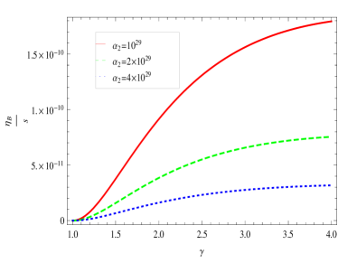
Figure 1: Plot of baryon to entropy ratio $\frac{\eta_{B}}{S}$ versus $\gamma$ for Model I for different values of $\alpha_{2}$, other parameters are $g_{b}=1,~{}\mathcal{T}_{D}=2\times 10^{16},~{}M_{\ast}=10^{12},~{}g_{\ast}=106,~{}\kappa=1$ and $\alpha_{1}=2\times 10^{39}$.

In Figure 1, we plot baryon to entropy ratio in terms of parameter $\gamma$ for different values of $\alpha_{2}$. For $\alpha_{2}=10^{29}$ and $\gamma=2$, we can see baryon to entropy ratio is confined to $\frac{\eta_{B}}{S}=8.9\times 10^{-11}$, also showing compatibility with observations. For other values of $\alpha_{2}$, we obtain results which are compatible with the observational value. Following Table 1 shows the different approach of baryon to entropy ratio for $\gamma=2,~{}3,~{}4$.

Table 1: Baryogenesis for $f(T,T_{G})=\alpha_{1}\sqrt{T^{2}+\alpha_{2}T_{G}}-T$

$\alpha_{2}$	$\gamma$	$\frac{\eta_{B}}{S}$ (Baryon to entropy ratio)
$10^{29}$	$2$	$8.9\times 10^{-11}$
$2\times 10^{29}$	$3$	$6.5\times 10^{-11}$
$4\times 10^{29}$	$4$	$3.1\times 10^{-11}$

III.2 Model II

This model is obtained from previous model by adding higher order correction terms $T^{2}$ and $T\sqrt{\mid T_{G}\mid}$. For this model, we also find the expressions $f_{T}$, $f_{T_{G}}$ and $\dot{f}_{T_{G}}$, which are obtained as

$$f_{T} = -1+\frac{12\alpha_{1}\gamma^{2}}{t^{2}}+\frac{6\beta_{1}}{\sqrt{36+24\beta_{2}-\frac{24\beta_{2}}{\gamma}}}+\frac{\alpha_{2}\gamma^{2}\sqrt{|24-\frac{24}{\gamma}|}}{t^{2}},$$ (32)

$$f_{T_{G}} = \frac{\beta_{1}\beta_{2}t^{2}}{2\gamma^{2}\sqrt{36+24\beta_{2}-\frac{24\beta_{2}}{\gamma}}}+\frac{3\alpha_{2}}{\sqrt{|24-\frac{24}{\gamma}|}},$$ (33)

$$\dot{f}_{T_{G}} = \frac{36\beta_{1}\beta_{2}t}{\gamma^{2}\bigg{(}36+24\beta_{2}-\frac{24\beta_{2}}{\gamma}\bigg{)}^{\frac{3}{2}}}+\frac{24\beta_{1}\beta_{2}^{2}(1-\frac{1}{\gamma})t}{\gamma^{2}\bigg{(}36+24\beta_{2}-\frac{24\beta_{2}}{\gamma}\bigg{)}^{\frac{3}{2}}}.$$ (34)

Substituting these expressions in Eq. (12), we have

$$\rho = \frac{1}{2\kappa^{2}t^{2}}\bigg{(}6\gamma^{2}+\beta_{1}\gamma^{2}A-\frac{72\beta_{1}\gamma^{2}}{A}-\frac{\beta_{1}\beta_{2}\gamma^{4}\zeta^{2}}{2A}+\frac{864\beta_{1}\beta_{2}\gamma}{A^{3}}+\frac{24\beta_{1}\beta_{2}^{2}\gamma\zeta^{2}}{A^{3}}\bigg{)}$$ (35)

$$- \frac{1}{2\kappa^{2}t^{4}}\bigg{(}108\alpha_{1}\gamma^{4}+9\alpha_{2}\gamma^{4}\zeta\bigg{)},$$

where $\zeta=\sqrt{|24-\frac{24}{\gamma}|}$. Comparing Eqs. (18) with (35), we obtain $t_{D}$ as

$$t_{D}=\left(\frac{c_{1}+\sqrt{c_{1}^{2}-\frac{4\kappa^{2}\pi^{2}g_{\ast}c_{2}\mathcal{T}_{D}^{4}}{15}}}{\frac{2\kappa^{2}\pi^{2}g_{\ast}\mathcal{T}_{D}^{4}}{15}}\right)^{\frac{1}{2}},$$ (36)

where $c_{1}=6\gamma^{2}+\beta_{1}\gamma^{2}A-\frac{72\beta_{1}\gamma^{2}}{A}-\frac{\beta_{1}\beta_{2}\gamma^{4}\zeta^{2}}{2A}+\frac{864\beta_{1}\beta_{2}\gamma}{A^{3}}+\frac{24\beta_{1}\beta_{2}^{2}\gamma\zeta^{2}}{A^{3}}$ and $c_{2}=108\alpha_{1}\gamma^{4}+9\alpha_{2}\gamma^{4}\zeta$. Using Eq.(36), we obtain the final expression for this particular model as

$$\frac{\eta_{B}}{S} \simeq \frac{45g_{b}\gamma^{2}\kappa^{3}\pi\mathcal{T}_{D}^{5}}{g_{*}M_{*}^{2}}\bigg{(}1+\frac{16\kappa^{2}\pi^{2}g_{\ast}\mathcal{T}_{D}^{4}\gamma(\gamma-1)}{15\bigg{(}c_{1}+\sqrt{c_{1}^{2}-\frac{4\kappa^{2}\pi^{2}g_{\ast}c_{2}\mathcal{T}_{D}^{4}}{15}}\bigg{)}}\bigg{)}\bigg{(}\sqrt{c_{1}^{2}-\frac{4\kappa^{2}\pi^{2}g_{\ast}c_{2}\mathcal{T}_{D}^{4}}{15}}+c_{1}\bigg{)}^{-\frac{3}{2}}$$ (37)

$$\times \bigg{(}\frac{2g_{\ast}}{15}\bigg{)}^{\frac{3}{2}}.$$

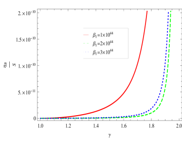
Figure 2: The behavior of baryon to entropy ratio $\frac{\eta_{B}}{S}$ versus $\gamma$ for Model II, for $g_{b}=1,~{}\mathcal{T}_{D}=2\times 10^{16},~{}M_{\ast}=10^{12},~{}g_{\ast}=106,~{}\kappa=1,~{}\alpha_{1}=2\times 10^{-20},~{}\alpha_{2}=2\times 10^{20}$ and $\beta_{2}=10^{20}$.

Figure 2 illustrates the dependence of the baryon to entropy ratio on the dimensionless parameter $\gamma$ for Model II. We notice that when $1.65\leq\gamma\leq 1.94$, we obtain $\frac{\eta_{B}}{S}$ in leading order as $7.5^{+1.5}_{-1.1}\times 10^{-11}$ which is compatible with observational bounds. Following table describes the detailed discussion of Figure 2.

Table 2: Baryogenesis for $f(T,T_{G})=\alpha_{1}T^{2}+\alpha_{2}T\sqrt{\mid T_{G}\mid}+\beta_{1}\sqrt{T^{2}+\beta_{2}T_{G}}-T$

$\beta_{1}$	$\gamma$	$\frac{\eta_{B}}{S}$ (Baryon to entropy ratio)
$10^{44}$	$1.65$	$6.9\times 10^{-11}$
$2\times 10^{44}$	$1.9$	$7\times 10^{-11}$
$3\times 10^{44}$	$1.87$	$7.2\times 10^{-11}$

III.3 Model III

Bahamonde and Capozziello 26 investigated this model by considering $g(B)=f_{1}B\ln B$ where $f_{1}$ is an arbitrary constant. So expressions $f_{T},~{}f_{B}$ and $\dot{f}_{B}$, for this model will be as follows

$$f_{T}=-1,\quad f_{B}=f_{1}\left(1+\ln\left(\frac{6\gamma(3\gamma-1)}{t^{2}}\right)\right),\quad\dot{f}_{B}=\frac{-2f_{1}}{t}.$$ (38)

Now, one can find the energy density of ordinary matter $\rho(t)$ by using Eqs. (21) and (38)

$$\rho(t)=\frac{1}{\kappa^{2}t^{2}}\left(3\gamma^{2}-3\gamma f_{1}-9\gamma^{2}f_{1}\right).$$ (39)

Using Eqs.(18) and (39), we get $t_{D}$ as

$$t_{D}=\frac{3\sqrt{10}}{\kappa\pi\mathcal{T}_{D}^{2}}\sqrt{\frac{\gamma\left(\gamma-3f_{1}\gamma-f_{1}\right)}{g_{\ast}}}.$$ (40)

Now expression of baryon to entropy ratio can be obtained by using Eqs. (21), (23), (25) and (40) as follow

$$\frac{\eta_{B}}{S}\simeq\frac{\kappa^{3}\pi\mathcal{T}_{D}^{5}(4\gamma-1)g_{b}\sqrt{g_{\ast}}}{6\sqrt{10}M_{\ast}^{2}\gamma^{\frac{1}{2}}\left(\gamma-3f_{1}\gamma-f_{1}\right)^{\frac{3}{2}}}.$$ (41)

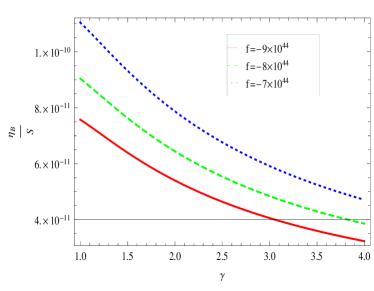
Figure 3: Plot of $\frac{\eta_{B}}{S}$ as the function of $\gamma$ for Model III, we take $g_{b}=1,~{}\mathcal{T}_{D}=2\times 10^{16},~{}M_{\ast}=10^{12},~{}g_{\ast}=106,~{}\kappa=1$.

In Figure 3, we plot the baryon to entropy ratio against parameter $\gamma$. As it can be seen when $\gamma\leq 1.56$, baryon to entropy ratio lies in the range $7.5^{+1.5}_{-1.5}\times 10^{-11}$, which favors the observational value. Table III indicates the different cases of baryon to entropy ratio.

Table 3: Baryogenesis for $f(T,B)=-T+g(B)$

$f$	$\gamma$	$\frac{\eta_{B}}{S}$ (Baryon to entropy ratio)
$-9\times 10^{44}$	$1$	$7.5\times 10^{-11}$
$-8\times 10^{44}$	$1$	$9\times 10^{-11}$
$-7\times 10^{44}$	$1.5$	$9.3\times 10^{-11}$

III.4 Model IV

First we consider a general Taylor expansion of the $f(T,B)$ Lagrangian 25a as

$$f(T,B) = f(T_{0},B_{0})+f_{T}(T_{0},B_{0})(T-T_{0})+f_{B}(T_{0},B_{0})(B-B_{0})+\frac{1}{2!}f_{TT}$$ (42)

$$\times (T_{0},B_{0})(T-T_{0})^{2}+\frac{1}{2!}f_{BB}(T_{0},B_{0})(B-B_{0})^{2}+f_{TB}(T_{0},B_{0})(T$$

$$- T_{0})(B-B_{0})+\mathcal{O}(T^{3},B^{3}),$$

Since boundary term $B$ has linear order, so consider $T_{0}=B_{0}=0$, by taking constants $A_{i}$, the Lagrangian can be written as

$$f(T,B)=A_{0}+A_{1}T+A_{2}T^{2}+A_{3}B^{2}+A_{4}TB.$$ (43)

Next, we find the expressions $f_{T}$, $f_{B}$ and $\dot{f}_{B}$, which lead to

$$f_{T} = A_{1}+\frac{12A_{2}\gamma^{2}}{t^{2}}+\frac{6A_{4}\gamma(3\gamma-1)}{t^{2}},$$ (44)

$$f_{B} = \frac{12A_{3}\gamma(3\gamma-1)}{t^{2}}+\frac{6A_{4}\gamma^{2}}{t^{2}},$$ (45)

$$\dot{f}_{B} = -\frac{24A_{3}\gamma(3\gamma-1)}{t^{3}}-\frac{12A_{4}\gamma^{2}}{t^{3}}.$$ (46)

Using Eqs. (21), (44), (45) and (46), on can write the energy density $\rho(t)$ in a radiation dominated universe as

$$\rho(t) = \frac{1}{\kappa^{2}t^{4}}\left(-162A_{3}\gamma^{4}-108A_{3}\gamma^{3}-108A_{4}\gamma^{4}-54A_{2}\gamma^{4}+54A_{3}\gamma^{2}\right)-\frac{3A_{1}\gamma^{2}}{\kappa^{2}t^{2}}+\frac{A_{0}}{2\kappa^{2}}.$$ (47)

Decoupling cosmic time for this case, will be

$$t_{D}=\left(\frac{2\chi}{3A_{1}\gamma^{2}+\sqrt{9A_{1}^{2}\gamma^{4}+2\chi\left(\frac{\kappa^{2}\pi^{2}g_{\ast}\mathcal{T}_{D}^{4}}{15}-A_{0}\right)}}\right)^{\frac{1}{2}},$$ (48)

where $\chi=-162A_{3}\gamma^{4}-108A_{3}\gamma^{3}-108A_{4}\gamma^{4}-54A_{2}\gamma^{4}+54A_{3}\gamma^{2}$. In this case, baryon to entropy ration will be

$$\frac{\eta_{B}}{S}=\frac{45g_{b}\gamma(4\gamma-1)}{\pi^{2}g_{\ast}M_{\ast}^{2}\mathcal{T}_{D}}\left(\frac{3A_{1}\gamma^{2}+\sqrt{9A_{1}^{2}\gamma^{4}+2\chi\left(\frac{\kappa^{2}\pi^{2}g_{\ast}\mathcal{T}_{D}^{4}}{15}-A_{0}\right)}}{2\chi}\right)^{\frac{3}{2}}.$$ (49)

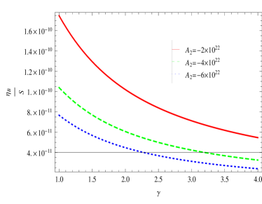
Figure 4: Plot of baryon to entropy ratio $\frac{\eta_{B}}{S}$ against $\gamma$ for Model IV, for $g_{b}=1,~{}\mathcal{T}_{D}=2\times 10^{16},~{}M_{\ast}=10^{12},~{}g_{\ast}=106,~{}\kappa=1,~{}A_{0}=2\times 10^{10},~{}A_{1}=3\times 10^{10},~{}A_{3}=5\times 10^{10}$ and $A_{4}=6\times 10^{10}$.

Figure 4 yields the baryon to entropy ratio verses $\gamma$ in the framework of $f(T,B)$-gravity with general Taylor expansion model for different values of $A_{2}$. One can see that for $A_{2}=-2\times 10^{22}$, before $\gamma=2.5$, baryon to entropy ratio is $5.5\times 10^{-11}\leq\frac{\eta_{B}}{S}\leq 8.09\times 10^{-11}$. Moreover, for other cases when $\gamma\geq 1.25$, the trajectories are ruled out by observationally measured value of $\frac{\eta_{B}}{S}$. Table IV also summarizes some values of baryon to entropy ratio for $\gamma=1,~{}1.1,~{}2$

Table 4: Baryogenesis for $f(T,B)=A_{0}+A_{1}T+A_{2}T^{2}+A_{3}B^{2}+A_{4}TB$

$A_{2}$	$\gamma$	$\frac{\eta_{B}}{S}$ (Baryon to entropy ratio)
$-2\times 10^{22}$	$2$	$9\times 10^{-11}$
$-4\times 10^{22}$	$1.1$	$9\times 10^{-11}$
$-6\times 10^{22}$	$1$	$7.99\times 10^{-11}$

IV Generalized Baryogenesis Interaction

In this section, we present the more complete and generalized baryogenesis interaction in the framework of $f(T,T_{G})$-gravity 23aaa ; 19 . For this case CP-violation interaction proportional to $\partial_{\mu}f(T+T_{G})$, can be written as

$$\frac{1}{M_{\ast}}\int{\sqrt{-g}d^{4}x(\partial_{\mu}f(T+T_{G}))J^{\mu}}.$$ (50)

For this kind of baryogenesis interaction, baryon to entropy ratio will be as follows

$$\frac{\eta_{B}}{S}\simeq-\frac{15g_{b}}{4\pi^{2}g_{*}}\left(\frac{\dot{T}f_{T}+\dot{T}_{G}f_{T_{G}}}{M_{*}^{2}\mathcal{T}}\right)|_{\mathcal{T}_{D}}.$$ (51)

For this case CP-violation interaction term in the framework of $f(T,B)$-gravity written as

$$\frac{1}{M_{\ast}}\int{\sqrt{-g}d^{4}x(\partial_{\mu}f(T+B))J^{\mu}}.$$ (52)

Using Eq. (52), baryon to entropy ratio is given by

$$\frac{\eta_{B}}{s}\simeq-\frac{15g_{b}}{4\pi^{2}g_{*}}\left(\frac{\dot{T}f_{T}+\dot{B}f_{B}}{M_{*}^{2}\mathcal{T}}\right)|_{\mathcal{T}_{D}}.$$ (53)

IV.1 Model I

Using Eqs. (30) and (51), we have the following expression of baryon to entropy ratio

$$\frac{\eta_{B}}{S} = \frac{45g_{b}\kappa^{3}\pi\mathcal{T}_{D}^{5}\gamma}{g_{\ast}M_{\ast}^{2}}\left(\frac{6\gamma\alpha_{1}}{A}+\frac{4(\gamma-1)\alpha_{1}\alpha_{2}}{A}-\gamma\right)\bigg{(}\frac{15}{g_{\ast}}\bigg{(}6\gamma^{2}+A\gamma^{2}\alpha_{1}$$

$$- \frac{72\gamma^{2}\alpha_{1}}{A}-\frac{12\gamma(\gamma-1)\alpha_{1}\alpha_{2}}{A}\frac{864\gamma\alpha_{1}\alpha_{2}}{A^{3}}+\frac{576\alpha_{1}\alpha_{2}^{2}(\gamma-1)}{A^{3}}\bigg{)}\bigg{)}^{-\frac{3}{2}}.$$

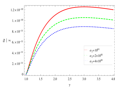
Figure 5: Plot of baryon to entropy ratio $\frac{\eta_{B}}{S}$ versus $\gamma$ for generalized baryogenesis interaction for Model I for different values of $\alpha_{2}$, with $g_{b}=1,~{}\mathcal{T}_{D}=2\times 10^{16},~{}M_{\ast}=10^{12},~{}g_{\ast}=106,~{}\kappa=1$ and $\alpha_{1}=10^{94}$.

In case of generalized baryogenesis interaction, the graph of baryon to entropy ratio verses $\gamma$ parameter is shown in Figure 5 for different values of $\alpha_{2}$. Thus three different cases can be distinguished as

• For $\alpha_{2}=10^{81}$ and $1.15\lesssim\gamma\lesssim 1.5$, we have $2\times 10^{-11}\lesssim\frac{\eta_{B}}{S}\lesssim 7.5\times 10^{-11}$.

• For $\alpha_{2}=2\times 10^{81}$ and $1.15\lesssim\gamma\lesssim 2$, then baryon to entropy ratio lies in the range $2\times 10^{-11}\lesssim\frac{\eta_{B}}{S}\lesssim 9.4\times 10^{-11}$.

• For $\alpha_{2}=4\times 10^{81}$ and $1.15\lesssim\gamma\lesssim 2.5$, we have $2\times 10^{-11}\lesssim\frac{\eta_{B}}{S}\lesssim 8.6\times 10^{-11}$.

All constraints are very close to the observationally accepted value. Other cases of baryon to entropy ratio are discussed in Table V.

Table 5: Generalized Baryogenesis Interaction for $f(T,T_{G})=\alpha_{1}\sqrt{T^{2}+\alpha_{2}T_{G}}-T$

$\alpha_{2}$	$\gamma$	$\frac{\eta_{B}}{S}$ (Baryon to entropy ratio)
$10^{81}$	$1.5$	$7.5\times 10^{-11}$
$2\times 10^{81}$	$2$	$9.4\times 10^{-11}$
$4\times 10^{81}$	$2.5$	$8.6\times 10^{-11}$

IV.2 Model II

For generalized baryogenesis interaction case, the baryon to entropy ratio (51) for this specific model become

$$\frac{\eta_{B}}{S} = \frac{45g_{b}\gamma^{2}\kappa^{3}\pi\mathcal{T}_{D}^{5}}{g_{*}M_{*}^{2}}\bigg{(}\frac{2g_{\ast}}{15}\bigg{)}^{\frac{3}{2}}\bigg{(}c_{1}+\sqrt{c_{1}^{2}-\frac{4\kappa^{2}\pi^{2}g_{\ast}c_{2}\mathcal{T}_{D}^{4}}{15}}\bigg{)}^{-\frac{3}{2}}\bigg{(}\frac{6\beta_{1}}{A}$$ (55)

$$+ \frac{2\beta_{1}\beta_{2}(\gamma-1)}{A\gamma}+\frac{\left(2\kappa^{2}\pi^{2}g_{\ast}\mathcal{T}_{D}^{4}\right)\left(12\alpha_{1}\gamma^{2}+\alpha_{2}\gamma^{2}\zeta+\frac{12\alpha_{2}\gamma(\gamma-1)}{\zeta}\right)}{15\left(c_{1}+\sqrt{c_{1}^{2}-\frac{4\kappa^{2}\pi^{2}g_{\ast}\mathcal{T}_{D}^{4}c_{2}}{15}}\right)}\bigg{)}.$$

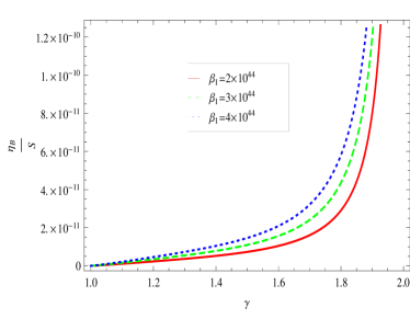
Figure 6: Plot of baryon to entropy ratio $\frac{\eta_{B}}{S}$ against $\gamma$ in the context of generalized baryogenesis interaction for Model II, in this case $g_{b}=1,~{}\mathcal{T}_{D}=2\times 10^{16},~{}M_{\ast}=10^{12},~{}g_{\ast}=106,~{}\kappa=1,~{}\alpha_{1}=2\times 10^{40},~{}\alpha_{2}=2\times 10^{70}$ and $\beta_{2}=10^{90}$.

Graphical behavior of Eq. (55) is shown in Figure 6 for different values of $\beta_{1}$, one can notice all trajectories are correspond to $\frac{\eta_{B}}{S}=7.9\times 10^{-11}$ when $\gamma=1.9$, $\gamma=1.85$ and $\gamma=1.83$ as mention in following Table VI.

Table 6: Generalized Baryogenesis Interaction for $f(T,T_{G})=\alpha_{1}T^{2}+\alpha_{2}T\sqrt{\mid T_{G}\mid}+\beta_{1}\sqrt{T^{2}+\beta_{2}T_{G}}-T$

$\beta_{1}$	$\gamma$	$\frac{\eta_{B}}{S}$ (Baryon to entropy ratio)
$2\times 10^{44}$	$1.9$	$7.9\times 10^{-11}$
$3\times 10^{44}$	$1.85$	$7.9\times 10^{-11}$
$4\times 10^{44}$	$1.83$	$7.9\times 10^{-11}$

IV.3 Model III

Using Eqs. (40) and (53), we obtain the expression of baryon to entropy ratio

$$\frac{\eta_{B}}{S} \simeq \frac{\kappa^{3}\pi\mathcal{T}_{D}^{5}g_{b}\sqrt{g_{\ast}}}{6\sqrt{10}M_{\ast}^{2}\gamma^{\frac{1}{2}}(\gamma-3f_{1}\gamma-f_{1})^{\frac{3}{2}}}\bigg{(}(3\gamma-1)f\bigg{(}1+\ln\bigg{(}\frac{\gamma(3\gamma-1)\kappa^{2}\pi^{2}\mathcal{T}_{D}^{4}g_{\ast}}{90\gamma(\gamma-3f\gamma-f)}\bigg{)}\bigg{)}-\gamma\bigg{)}.$$ (56)

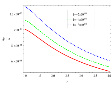
Figure 7: Plot of baryon to entropy ratio $\frac{\eta_{B}}{S}$ as the function of parameter $\gamma$ in the framework of generalized baryogenesis interaction for Model III, we set the values of parameters as $g_{b}=1,~{}\mathcal{T}_{D}=2\times 10^{16},~{}M_{\ast}=10^{12},~{}g_{\ast}=106,~{}\kappa=1$.

In Figure 7, we plot $\gamma$-dependence of the baryon to entropy ratio for different values of values of $f$. It informs us that, for all values of $f$ by setting $\gamma=1.4,1.7,2.2$, we obtain baryon to entropy ratio as $\frac{\eta_{B}}{S}=9.2\times 10^{-11}$, which satisfy the observational constraints.

Table 7: Generalized Baryogenesis Interaction for $f(T,B)=-T+g(B)$

$f$	$\gamma$	$\frac{\eta_{B}}{S}$ (Baryon to entropy ratio)
$-5\times 10^{138}$	$1.4$	$9.2\times 10^{-11}$
$-4\times 10^{138}$	$1.7$	$9.2\times 10^{-11}$
$-3\times 10^{138}$	$2.2$	$9.2\times 10^{-11}$

IV.4 Model IV

In the context of more complete generalized baryogenesis interaction for this particular model,m we obtain the expression of baryon to entropy ratio as

$$\frac{\eta_{B}}{S} = \frac{45\gamma g_{b}}{2\pi^{2}g_{\ast}M_{\ast}^{2}\mathcal{T}_{D}}\left(\frac{\sqrt{9A_{1}^{2}\gamma^{4}+2\chi\left(\frac{\kappa^{2}\pi^{2}g_{\ast}\mathcal{T}_{D}^{4}}{15}-A_{0}\right)}}{2\chi}+\frac{3A_{1}\gamma^{2}}{2\chi}\right)^{\frac{5}{2}}\bigg{(}12\gamma^{3}A_{2}$$ (57)

$$+ \frac{2A_{1}\chi\gamma}{3A_{1}\gamma^{2}+\sqrt{9A_{1}^{2}\gamma^{4}+2\chi\left(\frac{\kappa^{2}\pi^{2}g_{\ast}\mathcal{T}_{D}^{4}}{15}-A_{0}\right)}}+18A_{4}\gamma^{2}(3\gamma-1)+24A_{3}$$

$$\times \gamma(3\gamma-1)^{2}\bigg{)}.$$

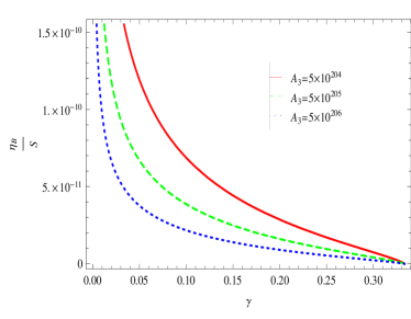
Figure 8: Plot of baryon to entropy ratio $\frac{\eta_{B}}{S}$ versus parameter $\gamma$ in the light of generalized baryogenesis interaction for Model IV. Other parameters are $g_{b}=1,~{}\mathcal{T}_{D}=2\times 10^{16},~{}M_{\ast}=10^{12},~{}g_{\ast}=106,~{}\kappa=1,~{}A_{0}=2\times 10^{10},~{}A_{1}=3\times 10^{10},~{}A_{2}=5\times 10^{70}$ and $A_{4}=6\times 10^{10}$.

It can be observed from Figure 8 that the baryon to entropy ratio remains $\frac{\eta_{B}}{S}\leq 9\times 10^{-11}$ for the range of $\gamma\geq 0.01$ which favors the observational bounds 1 ; 2 . Detailed discussion is mentioned in the following Table VIII.

Table 8: Generalized Baryogenesis interaction for $f(T,B)=A_{0}+A_{1}T+A_{2}T^{2}+A_{3}B^{2}+A_{4}TB$

$A_{3}$	$\gamma$	$\frac{\eta_{B}}{S}$ (Baryon to entropy ratio)
$5\times 10^{204}$	$0.07$	$8.99\times 10^{-11}$
$5\times 10^{205}$	$0.03$	$8.8\times 10^{-11}$
$5\times 10^{206}$	$0.01$	$8.8\times 10^{-11}$

V Conclusion

This paper presented the detailed discussion of gravitational baryogenesis mechanism in the context of $f(T,T_{G})$ and $f(T,B)$ theories of gravity. For $f(T,T_{G})$-gravity, we have used two specific models $f(T,T_{G})=\alpha_{1}\sqrt{T^{2}+\alpha_{2}T_{G}}-T$ and $f(T,T_{G})=\alpha_{1}T^{2}+\alpha_{2}T\sqrt{|T_{G}|}+\beta_{1}\sqrt{T^{2}+\beta_{2}T_{G}}-T$. Similarly, we considered $f(T,B)=-T+g(B)$ where ($g(B)=f_{1}B\ln B$) and $f(T,B)=A_{0}+A_{1}T+A_{2}T^{2}+A_{3}B^{2}+A_{4}TB$ models in the framework of $f(T,B)$-gravity. For both theories of gravity, we have chosen scale factor $a(t)=m_{0}t^{\gamma}$ and constructed baryon to entropy ratio $\frac{\eta_{B}}{S}$ by assuming that the universe filled by perfect fluid and dark energy. We also evaluated more complete and generalized baryogenesis interaction proportional to $\partial_{\mu}f(T+T_{G})$ and $\partial_{\mu}f(T+B)$. For all cases, our results have showed excellent consistency with approximate observational value $\frac{\eta_{B}}{S}\sim 9.42\times 10^{-11}$ 1 ; 2 . The core results of this work are given below.

• Model I: In Figure 1, we show the plot of baryon to entropy ratio against parameter $\gamma$, which shows that observation value of baryon to entropy ratio can be met for $\gamma\leq 2$ with $\alpha_{2}=10^{29}$.

• Model II: In Figure 2, One can find the value of baryon to entropy ratio approximately equal to $7.5^{+1.5}_{-1.1}\times 10^{-11}$ with $1.65\leq\gamma\leq 1.94$ for all cases of $\beta_{1}$, which satisfied the observational bounds.

• Model III: It is observed that $\gamma\leq 1.56$, for all values of $f$, our result $\frac{\eta_{B}}{S}=7.5^{+1.5}_{-1.5}\times 10^{-11}$ correspond to observationally measured value of baryon to entropy ratio (Figure 3).

• Model IV: For this model, we observed (Figure 4) $5.5\times 10^{-11}\leq\frac{\eta_{B}}{S}\leq 8.09\times 10^{-11}$, before $\gamma=2.5$ and $A_{2}=-2\times 10^{22}$, which indicate the excellent agreement with observational value $\frac{\eta_{B}}{S}\sim 9.42\times 10^{-11}$. Anyhow, for other values of $A_{2}$ and $\gamma\geq 1.25$, trajectories are very close to observational constraints.

  In the following, we have given the results for the generalized Baryogenesis interaction scenario. These are as follows:

• Model I: For this baryogenesis interaction (Figure 5), for $\alpha_{2}=10^{81}$ and $1.15\lesssim\gamma\lesssim 1.5$, the ratio of baryon number density to entropy obtained by gravitational baryogenesis (LABEL:ali3) lies in the range $2\times 10^{-11}\lesssim\frac{\eta_{B}}{S}\lesssim 7.5\times 10^{-11}$. While for $\alpha_{2}=2\times 10^{81}$ and $1.15\lesssim\gamma\lesssim 2$. this ratio correspond to $2\times 10^{-11}\lesssim\frac{\eta_{B}}{S}\lesssim 9.4\times 10^{-11}$. Similarly, for $\alpha_{2}=4\times 10^{81}$ and $1.15\lesssim\gamma\lesssim 2.5$, we have $2\times 10^{-11}\lesssim\frac{\eta_{B}}{S}\lesssim 8.6\times 10^{-11}$.

• Model II: For this model, the baryon to entropy ratio at leading order is, $\frac{\eta_{B}}{S}=7.9\times 10^{-11}$ for all cases when $1.83\leq\gamma\leq 1.9$, which is in very good agreement with observations (Figure 6).

• Model III: From the curves of the Figure 7, we notice that for $\gamma=1.4,1.7,2.2$, implies $\frac{\eta_{B}}{S}=9.2\times 10^{-11}$, which compatible with the observation data of baryon to entropy ratio.

• Model IV: For this model, our result is shown in Figure 8, which provides a well matched observational value when $\gamma\geq 0.01$.

References

- (1) C. L. Bennett et al., WMAP Collaboration, Astrophys. J. Suppl. 148, 1 (2003).
- (2) S. Burles, K. M. Nollett and M. S. Turner, Phys. Rev. D 63, 063512 (2001).
- (3) E. D. Stewart et al., Phys. Rev. D. 54, 6032 (1996).
- (4) M. Yamada, Phys. Rev. D 93, 083516 (2016).
- (5) K. Akita et al., J. Cosmol. Astropart. Phys. 04, 042 (2017).
- (6) M. Trodden, Rev. Mod. Phys. 71, 1463 (1999).
- (7) D. E. Morrissey and M. J. Ramsey-Musolf, New J. Phys. 14, 125003 (2012).
- (8) E. W. Kolb, et al., Phys. Rev. Lett. 77, 4290 (1996).
- (9) F. Takahashi and M. Yamaguchi, Phys. Rev. D 69, 083506 (2004).
- (10) R. H. Brandenberger and M. Yamaguchi, Phys. Rev. D 68, 023505 (2003).
- (11) A. D. Simone and T. Kobayashi, JCAP 08, 052 (2016).
- (12) A. D. Dolgov, Phys. Rev. D 24, 1042 (1981).
- (13) A. D. Sakharov, JETP Letters 5, 24 (1967).
- (14) H. Davoudiasl et al., Phys. Rev. Lett. 93, 201301 (2004).
- (15) K. Nozari and F. Rajabi, Commun. Theor. Phys. 70, 451 (2018).
- (16) D. Boulware and S. Deser, Phys. Rev. Lett. 55, 2656 (1985); J. T. Wheeler, Nucl. Phys. B 268, 737 (1986); I. Antoniadis, J. Rizos and K. Tamvakis, Nucl. Phys. B 415, 497 (1994); P. Kanti, J. Rizos and K. Tamvakis, Phys. Rev. D 59, 083512 (1999); N. E. Mavromatos and J. Rizos, Phys. Rev. D 62, 124004 (2000); S. Nojiri, S. D. Odintsov and M. Sasaki, Phys. Rev. D 71, 123509 (2005).
- (17) P. D. Mannheim and D. Kazanas, Astrophys. J. 342, 635 (1989); E. E. Flanagan, Phys. Rev. D 74, 023002 (2006); N. Deruelle, M. Sasaki, Y. Sendouda and A. Youssef, JCAP 1103, 040 (2011); D. Grumiller, M. Irakleidou, I. Lovrekovic and R. McNees, Phys. Rev. Lett. 112, 111102 (2014).
- (18) D. Lovelock, J. Math. Phys. 12, 498 (1971); N. Deruelle and L. Farina-Busto, Phys. Rev. D 41, 3696 (1990).
- (19) G. Kofinas and E. N. Saridakis, Phys. Rev. D 90, 084044 (2014); Phys. Rev. D 90, 084045 (2014); G. Kofinas, G. Leon and E. N. Saridakis, Class. Quantum Grav. 31, 175011 (2014).
- (20) S. Bahamonde, C. G. Bhmer and M. Wright, Phys. Rev. D 92, 104042 (2015).
- (21) S. Nojiri and S. D. Odintsov, Int. J. Geom. Meth. Mod. Phys. 4, 115 (2007).
- (22) S. Nojiri and S. D. Odintsov. Phys. Rept. 505, 59 (2011)
- (23) A. De Felice and S. Tsujikawa. Liv. Rev. Rel. 13, 03 (2010)
- (24) K. Bamba, S. Capozziello, S. Nojiri, and S. D. Odintsov. Astrophys. Space Sci. 345, 155 (2012).
- (25) S. Nojiri, S. D. Odintsov and V. K. Oikonomou, Phys. Rept. 692, 1-104 (2017).
- (26) V. K. Oikonomou, Int. J. Geom. Meth. Mod. Phys. 13 1650033 (2016).
- (27) S. D. Odintsov, V. K. Oikonomou, EPL 116, 49001 (2016).
- (28) M. P. L. P. Ramos and J. Paramos, Phys. Rev. D 96, 104024 (2017).
- (29) G. Lambiase and G. Scarpetta, Phys. Rev. D 74, 087504 (2006).
- (30) S. D. Odintsov and V. K. Oikonomou, Phys. Lett. B 760, 259 (2016).
- (31) V. K. Oikonomou and E. N. Saridakis, Phys. Rev. D 94, 124005 (2016).
- (32) M. C. Bento et al., Phys. Rev. D 71, 123517 (2005).
- (33) E. H. Baffou et al., Eur. Phys. J. C 79, 112 (2019).
- (34) P. K. Sahoo and S. Bhattacharjee, IJTP 59, 1451 (2020).
- (35) S. Bhattacharjee and P. K. Sahoo, Eur. Phys. J. C 80, 289 (2020).
- (36) S. Bhattacharjee, Phys. Dark Univ. 30, 100612 (2020).
- (37) M. Zubair and A. Jawad, Astrophys. Space Sci. 360, 11 (2015).
- (38) S. Nojiri and S. D. Odintsov, Phys. Lett. B 631, 1 (2005); A. De Felice and S. Tsujikawa, Phys. Lett. B 675, 1 (2009); S. C. Davis, Phys. Rev. D 67 024030 (2003); B. Eynard and N. Orantin, J. Phys. A: , 42, 29 (2009); A. De Felice and S. Tsujikawa, Phys. Rev. D 80, 063516 (2009); A. Jawad, S. Chattopadhyay and A. Pasqua, Eur. Phys. J. Plus 128, 88 (2013).
- (39) Petr V. Tretyakov, Mod. Phys. Lett. A 31, 14 (2016).
- (40) A. Paliathanasis, JCAP 1708, 027 (2017).
- (41) G. Farrugia, J. L. Said, V. Gakis and E. N. Saridakis, Phys. Rev. D 97, 124064 (2018).
- (42) S. Bahamonde, M. Zubair and G. Abbas, Phys. Dark Univ. 19, 78 (2018).
- (43) C. Escamilla-Rivera, J. L. Said, Class Quant Grav. 37, 16 (2020).
- (44) G. A. R. Franco, C. Escamilla-Rivera, J. L. Said, Eur. Phys. J. C 80, 677 (2020).
- (45) S. Bahamonde and S. Capozziello, Eur. Phys. J. C 77, 107 (2017).
- (46) G. Farrugia, J. L. Said, V. Gakis and E. N. Saridakis, Phys. Rev. D 97, 124064 (2018).