Dynamics of a two scalar field cosmological model with phantom terms

Abstract

We perform a detailed analysis on the dynamics of a Chiral-like cosmological model where the scalar fields can have negative kinetic terms. In particular, we study the asymptotic dynamics for the gravitational field equations for four different models in a spatially flat Friedmann–Lemaître–Robertson–Walker background space. When one of the scalar fields is phantom, we calculated that the cosmological fluid can evolves such that the parameter for the equation of state crosses twice the phantom divide line without the appearance of ghosts. Moreover, the cosmological viability of these four models is discussed.

I Introduction

The detailed analysis of recent observations Teg1 ; Teg2 ; Teg3 ; Teg4 ; Teg5 ; Teg6 ; Teg7 ; Teg8 ; Teg9 ; Teg10 ; Teg11 ; Teg12 supports the idea that the universe has gone under two acceleration phases during its evolution. An accelerated phase of expansion during its very early phase of evolution, known as inflation guth ; linde , which occurred prior to the radiation-dominated era; and a recently initiated accelerated phase of expansion, known as late time cosmic acceleration, driven by the so-called dark energy copeland ; Clifton1 ; Nojiri:2017ncd ; Ame10 ; Ame11 .

Within the framework of General Relativity, scalar fields play a significant role in gravitational physics because they provide theoretical mechanisms for the theoretical explanation of the observations. As inflaton is characterized by the scalar field that is responsible for the early time acceleration phase of the universe guth ; linde , the same model can provide dynamical terms in the gravitational field equations with antigravitating behaviour and can be used also as a model for the description of the acceleration of the late universe. The most well-known scalar field model which has been studied in the literature is the quintessence model Ratra ; qq1 ; qq2 ; qq3 ; qq4 ; qq5 ; qq6 . Alternative scalar-field models which have been proposed in the literature are: the phantom fields ph1 ; ph2 ; ph3 , the quintom model quin00 ; quin2 ; quin3 ; quin4 ; quin5 ; quin6 , the Chiral model ch1 ; ch2 ; ch3 ; ch4 , the k-essence scalar field model kes1 ; kes2 ; kes3 , Galileon giampero and many others hor1 ; hor2 ; hor3 .

An important common feature of the scalar-field models is that the gravitational field equations are of second-order, as in the case of General Relativity. Indeed, scalar fields introduce new degrees of freedom which are necessary in order to provide the necessary behaviour of the dynamics. Moreover these new degrees of freedom can attribute higher-order derivatives which are introduced in gravitational physics by theories of gravity alternatives of General Relativity so1 .

In this study we are interested in the study of the dynamics of a generalization of the Chiral cosmological model. The Chiral model belongs to the family of the multifield scalar-field theories, comprising two canonical scalar fields which interact in the kinetic and in the potential parts. In particular, the two scalar fields are involved in a two-dimensional space of negative constant curvature and Euclidean signature. There are various studies in the literature on this cosmological model ch1 ; ch2 ; ch3 ; ch4 with some interesting results. It has been shown that it can describe the whole dark sector of the universe, that is, it can been seen as a unified dark model for the description of the dark energy and of the dark matter an1 ; an2 . Moreover, it can provide two accelerated eras an3 , while, due to quantum transitions in the early universe, the physical fluid can cross the phantom divide line an4 . The latter is possible when the kinetic part of one of the two fields changes sign and has a phantom behaviour where the model can be seen as extension of the quintom theory where the one field is quintessence and the second field is phantom.

The global dynamics and the cosmological eras provided by the Chiral cosmology are studied in detail in an2 .  In the following Sections we perform a complete study on the asymptotic dynamics and behaviour for the cosmological field equations of Chiral-like cosmological models where now at least one or both of the scalar fields can be phantom and can have negative kinetic energy. The mathematical tools that we apply for this work are based on the $H-$normalization approach cop1 , where the field equations are written in terms of dimensionless variables and are expressed in terms of a algebraic-differential system of first-order gn1 ; gn2 ; gn3 . For the latter dynamical system the stationary points are determined, where any stationary point describe a specific exact solutions that is a specific era in the cosmological history. The stability of the stationary points is also investigated. Such an analysis provides important results of the viability of the background equations of a proposed cosmological model vb1 ; vb2 ; vb3 ; vb4 . The plan of the paper is as follows.

In Section II we present the cosmological model of our analysis. It is that of two-scalar fields which interact in the kinetic term, in particular the kinetic part defines a space of constant curvature but not necessarily of Euclidean signature. In Section III we rewrite the gravitational field equations by using dimensionless variables in the $H$-normalization approach. The main analysis of this work is presented in Section IV in which we investigate the existence of stationary points and the physical properties of the exact solutions at the stationary points. Finally, in Section V we summarize and we draw our conclusions.

II Field equations

For the Gravitational Theory of our consideration we consider a two-scalar field model of Chiral-like with Action Integral

$$S=\int\sqrt{-g}dx^{4}\left(R-\frac{\varepsilon_{\phi}}{2}g^{\mu\nu}\nabla_{\mu}\phi\nabla_{\nu}\phi-\frac{\varepsilon_{\psi}}{2}g^{\mu\nu}e^{\kappa\phi}\nabla_{\mu}\psi\nabla_{\nu}\psi-V\left(\phi\right)\right),$$ (1)

where for the background space we consider that of a spatially flat Friedmann–Lemaître–Robertson–Walker (FLRW) space with line element

$$ds^{2}=-dt^{2}+a^{2}\left(t\right)\left(dx^{2}+dy^{2}+dz^{2}\right).$$ (2)

Spacetime (2) admits a six-dimensional Killing algebra, which we assume is inherited by the scalar fields $\phi\left(x^{\nu}\right),~{}\psi\left(x^{\nu}\right)$. Thus $\phi=\phi\left(t\right)$ and $\psi=\psi\left(t\right)$. Parameters $\left(\varepsilon_{\phi},\varepsilon_{\psi}\right)$ are constants and take values $\left(\varepsilon_{\phi},\varepsilon_{\psi}\right)=\left(\pm 1,\pm 1\right)$, in the case for which $\left(\varepsilon_{\phi},\varepsilon_{\psi}\right)=\left(+1,+1\right)$ the Chiral model is recovered, while in the case for which  $\left(\varepsilon_{\phi},\varepsilon_{\psi}\right)=\left(+1,-1\right)$ with $\kappa=0$ the Action Integral (1) becomes that of the quintom theory. The parameter $\kappa$ is related with the curvature of the two-dimensional manifold defined by the kinetic parts of the scalar fields, which has the line element

$$ds^{2}\left(\phi,\psi\right)=\varepsilon_{\phi}d\phi^{2}+\varepsilon_{\psi}e^{\kappa\phi}d\psi^{2}$$ (3)

and curvature $R_{\left(\phi,\psi\right)}^{\left(2\right)}=-\frac{1}{2\varepsilon_{\phi}}\kappa^{2}$. The line element (3) describes an Einstein space of constant curvature, where $R_{\left(\phi,\psi\right)}^{\left(2\right)}<0$ when $\varepsilon_{\phi}>0$ and $R_{\left(\phi,\psi\right)}^{\left(2\right)}>0$ for $\varepsilon_{\phi}<0$.

For the line element (2) and from (1) it follows that the gravitational field equations are

$$-3H^{2}+\frac{\varepsilon_{\phi}}{2}\dot{\phi}^{2}+\frac{\varepsilon_{\psi}}{2}e^{\kappa\phi}\dot{\psi}^{2}+V\left(\phi\right)=0~{},$$ (4)

$$2\dot{H}+3H^{2}+\frac{\varepsilon_{\phi}}{2}\dot{\phi}^{2}+\frac{\varepsilon_{\psi}}{2}e^{\kappa\phi}\dot{\psi}^{2}-V\left(\phi\right)=0~{},$$ (5)

$$\varepsilon_{\phi}\left(\ddot{\phi}+3H\dot{\phi}\right)-\kappa\frac{\varepsilon_{\psi}}{2}e^{\kappa\phi}\dot{\psi}^{2}+V_{,\phi}\left(\phi\right)=0~{}$$ (6)

and

$$\ddot{\psi}+3H\dot{\psi}+\kappa\dot{\phi}\dot{\psi}=0~{},$$ (7)

where $H=\frac{\dot{a}}{a}$ is the Hubble function. The energy density $\rho_{eff}$  and the pressure $p_{eff}~{}$of the effective fluid source are defined as follows

$$\rho_{eff}=\frac{\varepsilon_{\phi}}{2}\dot{\phi}^{2}+\frac{\varepsilon_{\psi}}{2}e^{\kappa\phi}\dot{\psi}^{2}+V\left(\phi\right)~{},~{}$$ (8)

$$p_{eff}=\frac{\varepsilon_{\phi}}{2}\dot{\phi}^{2}+\frac{\varepsilon_{\psi}}{2}e^{\kappa\phi}\dot{\psi}^{2}-V\left(\phi\right)~{},$$ (9)

while the effective parameter of state is given by the expression

$$w_{eff}=\frac{p_{eff}}{\rho_{eff}}=\frac{\varepsilon_{\phi}\dot{\phi}^{2}+\varepsilon_{\psi}e^{\kappa\phi}\dot{\psi}^{2}-2V\left(\phi\right)}{\varepsilon_{\phi}\dot{\phi}^{2}+\varepsilon_{\psi}e^{\kappa\phi}\dot{\psi}^{2}+2V\left(\phi\right)}~{}.$$ (10)

We follow an2 and we rewrite the field equations (4), (7) by using the variables

$$\rho_{\phi}=\frac{\varepsilon_{\phi}}{2}\dot{\phi}^{2}+V\left(\phi\right)~{},~{}p_{\phi}=\frac{\varepsilon_{\phi}}{2}\dot{\phi}^{2}-V\left(\phi\right)~{},$$ (11)

$$\rho_{\psi}=\frac{\varepsilon_{\psi}}{2}e^{\kappa\phi}\dot{\psi}^{2}~{},~{}p_{\psi}=\frac{\varepsilon_{\psi}}{2}\varepsilon_{\psi}e^{\kappa\phi}\dot{\psi}^{2}~{},$$ (12)

that is,

$$3H^{2}=\rho_{\phi}+\rho_{\psi}~{},$$ (13)

$$2\dot{H}+3H^{2}=-\left(p_{\phi}+p_{\psi}\right)~{},$$ (14)

$$\dot{\rho}_{\phi}+3H\left(\rho_{\phi}+p_{\phi}\right)=\dot{\phi}\frac{\partial}{\partial\phi}p_{\psi}~{}$$ (15)

and

$$\dot{\rho}_{\psi}+3H\left(\rho_{\psi}+p_{\psi}\right)=-\dot{\phi}\frac{\partial}{\partial\phi}p_{\psi}~{}.$$ (16)

from which it is clear how the two scalar fields interact. As we mentioned above, the Chiral model can describe the whole dark sector of the universe, that is, the dark matter and the dark energy, and there are various observational results in the literature which support an interaction between these two fluids in1 ; in2 ; in3 ; in4 ; in5 ; in6 .

III Asymptotic dynamics

In order to continue with the study of dynamics for the field equations we define the new dimensionless variables an2

$$x=\frac{\dot{\phi}}{\sqrt{6}H}~{},~{}y=\frac{\sqrt{V\left(\phi\right)}}{\sqrt{3}H}~{},~{}z=\frac{e^{\frac{\kappa}{2}}\dot{\psi}}{\sqrt{6}}~{},~{}\lambda=\frac{V_{,\phi}}{V}$$ (17)

where the field equations (4), (7) are written in the equivalent form of the algebraic-differential system

$$\frac{dx}{d\ln a}=\frac{1}{2}\left(3\varepsilon_{\phi}x^{3}-3x\left(1+y^{2}-\varepsilon_{\psi}z^{2}\right)+\frac{\sqrt{6}}{\varepsilon_{\phi}}\left(\varepsilon_{\psi}\kappa z^{2}-\lambda y^{2}\right)\right)~{},$$ (18)

$$\frac{dy}{d\ln a}=\frac{1}{2}y\left(3\left(1-y^{2}+\varepsilon_{\phi}x^{2}+\varepsilon_{\psi}z^{2}\right)+\sqrt{6}\lambda x\right)~{},~{}$$ (19)

$$\frac{dz}{d\ln a}=\frac{1}{2}z\left(3\left(\varepsilon_{\phi}x^{2}-3-3y^{2}+\varepsilon_{\psi}z^{2}\right)-\sqrt{6}\kappa~{}x\right)~{}$$ (20)

and

$$\frac{d\lambda}{d\ln a}=\sqrt{6}x\lambda\left(\Gamma\left(\lambda\right)-1\right)~{},~{}\Gamma\left(\lambda\right)=\frac{V_{\phi\phi}V}{\left(V_{\phi}\right)^{2}}~{},$$ (21)

with algebraic constraint

$$1-\varepsilon_{\phi}x^{2}-y^{2}-\varepsilon_{\psi}z^{2}=0.$$ (22)

Because of the algebraic constraint (22) the dynamical system (18)-(21) can be reduced by one dimension into a three-dimensional system, while when $V\left(\phi\right)=V_{0}e^{\sigma\phi}$, $\sigma=const.,~{}$it follows $\Gamma\left(\lambda\right)=1$, which means that $\lambda=const$. Thus the final dynamical system has dimension two.

Furthermore, the parameter for the equation of state for the effective fluid is calculated to be

$$w_{eff}\left(x,y,z\right)=\varepsilon_{\phi}x^{2}-y^{2}+\varepsilon_{\psi}z^{2}.$$ (23)

What is important is to find the range of the variables $\left(x,y,z\right)$. For the model A with $\left(\varepsilon_{\phi},\varepsilon_{\psi}\right)=\left(+1,+1\right)$, variables $\left(x,y,z\right)$ are defined on the surface of the three-dimensional unitary sphere $S^{3}$. This is not true for the remainder of the models which are: model B with $\left(\varepsilon_{\phi},\varepsilon_{\psi}\right)=\left(+1,-1\right),~{}$ model C with $\left(\varepsilon_{\phi},\varepsilon_{\psi}\right)=\left(-1,+1\right)$ and model D where now $\left(\varepsilon_{\phi},\varepsilon_{\psi}\right)=\left(-1,-1\right)$. In these three models, the variables $\left(x,y,z\right)$ are not bounded.

IV Stationary points for Exponential potential

For the exponential potential, $V\left(\phi\right)=V_{0}e^{\sigma\phi}$, the dynamical system, (18)-(21), reduces to a two-dimensional system, where $y^{2}=1-\varepsilon_{\phi}x^{2}-\varepsilon_{\psi}z^{2}$. The stationary points are found to be

$$P_{1}^{\left(\pm\right)}=\left(\pm\frac{1}{\sqrt{\varepsilon_{\phi}}},0,0\right)~{},~{}P_{2}=\left(-\frac{\lambda}{\varepsilon_{\phi}\sqrt{6}},\sqrt{1-\frac{\lambda^{2}}{6\varepsilon_{\phi}}},0\right)~{}$$

and

$$P_{3}^{\left(\pm\right)}=\left(-\frac{\sqrt{6}}{\kappa+\lambda},\sqrt{\frac{\kappa}{\kappa+\lambda}},\pm\sqrt{\frac{\lambda\left(\kappa+\lambda\right)-6\varepsilon_{\phi}}{\varepsilon_{\psi}\left(\kappa+\lambda\right)^{2}}}\right)~{}\text{.}$$

At the stationary points $P_{1}^{\left(\pm\right)},~{}P_{2}$ only the scalar field $\phi$ contributes in the cosmological fluid, while the second field appears at the stationary points $P_{3}^{\left(\pm\right)}$.

We continue by studying in detail, the viability of the stationary points and their stability for the four models of our analysis.

IV.1 Model A $\left(\varepsilon_{\phi},\varepsilon_{\psi}\right)=\left(+1,+1\right)$

For the Chiral model with  $\left(\varepsilon_{\phi},\varepsilon_{\psi}\right)=\left(+1,+1\right)$ and for the exponential potential the asymptotic dynamics have been studied before in an3 . For a completeness of our study we reproduce these results. In this model the stationary points are $P_{1}^{\left(\pm\right)}\left(A\right)=\left(\pm 1,0,0\right)~{},~{}P_{2}\left(A\right)=\left(-\frac{\lambda}{\sqrt{6}},\sqrt{1-\frac{\lambda^{2}}{6}},0\right)$ and $P_{3}^{\left(\pm\right)}\left(A\right)=\left(-\frac{\sqrt{6}}{\kappa+\lambda},\sqrt{\frac{\kappa}{\kappa+\lambda}},\pm\sqrt{\frac{\lambda\left(\kappa+\lambda\right)-6}{\left(\kappa+\lambda\right)^{2}}}\right)$.

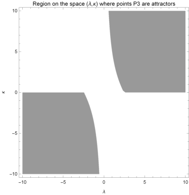
Figure 1: Region plots in the space of variables $\left(\lambda,\kappa\right)$ where the stationary points $P_{3}^{\left(\pm\right)}\left(A\right)~{}$are attractors.

Points $P_{1}^{\left(\pm\right)}\left(A\right)$ are always physically acceptable and describe universes in which only the kinetic part of the scalar field $\phi$ contributes in the total cosmological fluid. Indeed $w_{eff}\left(P_{1}^{\left(\pm\right)}\left(A\right)\right)=1$. This means that the stationary points describe stiff fluid solutions. The eigenvalues of the linearized system are $e_{1}\left(P_{1}^{\left(\pm\right)}\left(A\right)\right)=6\pm\sqrt{6}\lambda~{},~{}e_{2}\left(P_{1}^{\left(\pm\right)}\left(A\right)\right)=\mp\sqrt{\frac{3}{2}}\kappa$, from which we infer that $P_{1}^{\left(+\right)}\left(A\right)$ is an attractor for$\lambda<-\sqrt{6}$ and $\kappa>0$ while $P_{1}^{\left(-\right)}\left(A\right)$ is an attractor when $\lambda>\sqrt{6}$ and $\kappa<0$.

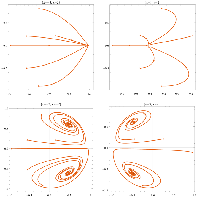
Figure 2: Phase space portrait in the space of variables $\left(x,z\right)$ for the dynamical system (18), (20) and for $\left(\varepsilon_{\phi},\varepsilon_{\psi}\right)=\left(+1,+1\right)$. The figures are for different values of the free parameters $\left\{\lambda,\kappa\right\}$. In the plots of the first row the unique attractor is point $P_{2}$, while in the second row the attractors are points $P_{3}^{\left(\pm\right)}$.

The stationary point $P_{2}\left(A\right)$ is physically acceptable for $\left|\lambda\right|<\sqrt{6}$. The point describes a scaling solution $w_{eff}\left(P_{2}\left(A\right)\right)=-1+\frac{\lambda^{2}}{3}$, from which it follows that $w_{eff}\left(P_{2}\left(A\right)\right)<-\frac{1}{3}$ if and only if $\left|\lambda\right|<\sqrt{2}$. The eigenvalues of the linearized system are determined to be $e_{1}\left(P_{2}\left(A\right)\right)=\frac{\left(\lambda^{2}-6\right)}{2}~{},~{}e_{2}\left(P_{2}\left(A\right)\right)=\frac{1}{2}\left(\lambda^{2}+\kappa\lambda-6\right)$. Thus the stationary point is an attractor when $\left\{-\sqrt{6}<\lambda<0,~{}\kappa>\frac{6-\lambda^{2}}{\lambda}\right\}~{}\cup~{}\left\{0<\lambda<\sqrt{6},\kappa<\frac{6-\lambda^{2}}{\lambda}\right\}\cup\left\{\lambda=0\right\}$.

Stationary points $P_{3}^{\left(\pm\right)}\left(A\right)$ are real and physically acceptable when $\left\{\lambda,\kappa\right\}$ are constrained as $\left\{\lambda\leq-\sqrt{6},\kappa<0\right\}\cup\left\{-\sqrt{6}<\lambda<0,\kappa<\frac{6-\lambda^{2}}{\lambda}\right\}$ and $\left\{0<\lambda<\sqrt{6},\kappa>\frac{6-\lambda^{2}}{\lambda}\right\}\cup\left\{\lambda\geq\sqrt{6},\kappa>0\right\}$. The effective fluid has equation of state $w_{eff}\left(P_{3}^{\left(\pm\right)}\left(A\right)\right)=1-\frac{2\kappa}{\kappa+\lambda}$, from which we infer that the exact solutions at the points describe accelerated universes when $\left\{\lambda\leq-\sqrt{2},\kappa<2\lambda\right\}\cup\left\{-\sqrt{2}<\lambda<0,\kappa<\frac{6-\lambda^{2}}{\lambda}\right\}$ and $\left\{0<\lambda<\sqrt{2},\kappa>\frac{6-\lambda^{2}}{\lambda}\right\}\cup\left\{\lambda\geq\sqrt{2},\kappa>2\lambda\right\}$. The eigenvalues of the linearized system around the stationary points $P_{3}^{\left(\pm\right)}\left(A\right)$ are derived as $e_{\pm}\left(P_{3}^{\left(\pm\right)}\left(A\right)\right)=-\frac{3\kappa}{2\left(\kappa+\lambda\right)}\pm\frac{i\sqrt{3\kappa}}{2\left(\kappa+\lambda\right)}\sqrt{\Delta}$, where $\Delta=4\lambda^{3}+8\kappa\lambda^{2}+\lambda\left(\kappa^{2}-6\right)-27\kappa$. The real part of eigenvalue, $e_{-}\left(P_{3}^{\left(\pm\right)}\left(A\right)\right),$ is always negative when $\frac{\kappa}{\left(\kappa+\lambda\right)}>0$. Thus in this case the stationary points can be saddles or attractors. The region plot in the space of the variables $\left(\lambda,\kappa\right)$, in which the exact solutions at the points $P_{3}^{\left(\pm\right)}\left(A\right)$ are stable, is presented in Fig. 1.

In Fig. 2 there are the phase space portraits in the space of variables $\left(x,z\right)$ for the dynamical system (18), (20). The figures are for different values of the free parameters $\left\{\lambda,\kappa\right\}$ so that to have different stationary points as attractors.

IV.2 Model B $\left(\varepsilon_{\phi},\varepsilon_{\psi}\right)=\left(+1,-1\right)$

For the model with $\left(\varepsilon_{\phi},\varepsilon_{\psi}\right)=\left(+1,-1\right)$ the admitted stationary points of the gravitational field equations are $P_{1}^{\left(\pm\right)}\left(B\right)=\left(\pm 1,0,0\right),~{}P_{2}\left(B\right)=\left(-\frac{\lambda}{\sqrt{6}},\sqrt{1-\frac{\lambda^{2}}{6}},0\right)$ and $P_{3}^{\left(\pm\right)}\left(B\right)=\left(-\frac{\sqrt{6}}{\kappa+\lambda},\sqrt{\frac{\kappa}{\kappa+\lambda}},\pm\sqrt{\frac{6-\lambda\left(\kappa+\lambda\right)}{\left(\kappa+\lambda\right)^{2}}}\right)$.

For the stationary Points $P_{1}^{\left(\pm\right)}\left(B\right)$ and $P_{2}\left(B\right)$ we find the same physical properties as with the corresponding points of model A. Furthermore, points $P_{3}^{\left(\pm\right)}\left(B\right)$ are real and physically acceptable when $\left\{\lambda\leq-\sqrt{6}~{},~{}\kappa>-\lambda\right\}\cup\left\{-\sqrt{6}<\lambda<0,~{}\kappa>-\lambda\text{ or }\frac{6-\lambda^{2}}{\lambda}<\kappa<0\right\}~{}$ and $\left\{0<\lambda<\sqrt{6},~{}\kappa<-\lambda\text{ or }0<\kappa<\frac{6-\lambda^{2}}{\lambda}\right\}\cup\left\{\lambda\subset\sqrt{6}~{},~{}\kappa<-\lambda\right\}$. The eigenvalues of the linearized system near the points $P_{3}^{\left(\pm\right)}\left(B\right)$ have the same functional form as points $P_{3}^{\left(\pm\right)}\left(A\right)$. Thus for this model the exact solutions at the stationary points are always unstable, while the stationary points are always saddle points.

Phase space portraits for the variables $\left(x,z\right)$ of the gravitational field equations for $\left(\varepsilon_{\phi},\varepsilon_{\psi}\right)=\left(+1,-1\right)$ are presented in Fig. 3, from where we observe that the unique attractor is point $P_{2}\left(B\right)$.

Figure 3: Phase space portrait in the space of variables $\left(x,z\right)$ for the dynamical system (18), (20) and for $\left(\varepsilon_{\phi},\varepsilon_{\psi}\right)=\left(+1,-1\right)$. The figures are for different values of the free parameters $\left\{\lambda,\kappa\right\}$. We observe that the unique attractor is point $P_{2}\left(B\right)$.

Figure 4: Qualitative evolution of $w_{eff}$ for the numerical solutions of the phase portraits in Fig. 3

In Fig. 4 we present the qualitative evolution for the parameter for the equation of state for the effective fluid,  $w_{eff}$, for the solutions presented in the phase space of Fig. 3. It is clear that the equation of state parameter can cross the phantom divide line twice. That is it can start from the $w_{eff}>-1$ then take values $w_{eff}<-1$ and cross again the limit and end with $w_{eff}>-1$.

It is important to mention here that in contrast to model A, the variables $\left(x,z\right)$ are not constrained and they can take values at .

IV.2.1 Analysis at infinity

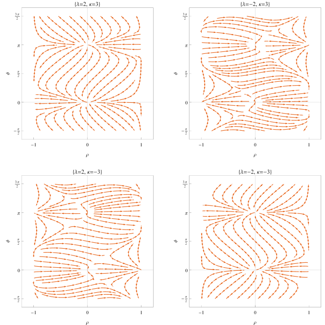
Figure 5: Phase space portrait in the space of variables $\left(\rho,v\right)$ for the dynamical system (25), (26). The figures are for different values of the free parameters $\left\{\lambda,\kappa\right\}$.

In order to perform the analysis at infinity we define the new variables

$$x=\frac{\cos u\cos v}{\rho}~{},~{}y=\frac{\cos u\sin v}{\rho}~{},~{}z=\frac{\sin u}{\rho}~{},$$ (24)

where when $\rho\rightarrow 0$, parameters $\left(x,y,z\right)$ have values at infinity. The constraint (22) becomes $\rho^{2}-\cos\left(2\theta\right)=0$, while the field equations reads

$$\rho^{\prime}=\frac{1}{2}\left(\sqrt{6\left(1-\rho^{4}\right)}\kappa\rho\cos v\sin\left(\frac{1}{2}\arccos\rho^{2}\right)-3\sin^{2}v\left(\rho^{4}-1\right)\right)~{},$$ (25)

$$v^{\prime}=\frac{1}{4}\left(12\rho\cos v+\sqrt{6}\left(\kappa+\lambda+\rho^{2}\left(\lambda-\kappa\right)\right)\frac{\sin v}{\cos\left(\frac{1}{2}\arccos\rho^{2}\right)}\right)~{},$$ (26)

where $\rho^{\prime}=\rho\frac{d\rho}{d\ln a}$. The stationary points $Q=\left(\rho,v\right)~{}$with $\rho=0$ are those with $v_{1}=0$ and $v_{2}=\pi$. The points with coordinates $Q_{1}=\left(0,0\right)$ and $Q_{2}=\left(0,\pi\right)$ provide physical solutions where only the kinetic parts of the scalar field contributes, that is, the physical solution describes a stiff fluid.

As far as the stability of the stationary points is concerned, it follows that $Q_{1}$ is an attractor when $\left\{\lambda<0,~{}\kappa<0\right\}$ or $\left\{\lambda>0,~{}\kappa<-\lambda\right\}$, while $Q_{2}$ is an attractor when $\left\{\lambda<0,~{}\kappa>-\lambda\right\}$ and $\left\{\lambda>0,\kappa>0\right\}$. In Fig. 5 we present the phase space portrait for the dynamical system (25), (26).

IV.3 Model C $\left(\varepsilon_{\phi},\varepsilon_{\psi}\right)=\left(-1,+1\right)$

In the case where $\phi$ is a phantom field, that is, $\left(\varepsilon_{\phi},\varepsilon_{\psi}\right)=\left(-1,+1\right)$, the real stationary points are the $P_{2}\left(C\right)=\left(\frac{\lambda}{\sqrt{6}},\sqrt{1+\frac{\lambda^{2}}{6}},0\right)$ and $P_{3}^{\left(\pm\right)}\left(C\right)=\left(-\frac{\sqrt{6}}{\kappa+\lambda},\sqrt{\frac{\kappa}{\kappa+\lambda}},\pm\sqrt{\frac{\lambda\left(\kappa+\lambda\right)+6}{\left(\kappa+\lambda\right)^{2}}}\right)$. The exact solution at point $P_{2}\left(C\right)$ describes a universe where the effective fluid has an equation of state parameter $w_{eff}=-1-\frac{\lambda^{2}}{3}$, which means that $w_{eff}<-1$, crosses the phantom divide line. On the other hand, points $P_{3}^{\left(\pm\right)}\left(C\right)$ have the same physical properties with points $P_{3}^{\left(\pm\right)}\left(A\right)$, while points are real when $\lambda\left(\kappa+\lambda\right)+6>0$, that is, $\left\{\lambda<0,\kappa<-\frac{6+\lambda^{2}}{\lambda}\right\}$ $\cup$ $\left\{\lambda>0,\kappa>-\frac{6+\lambda^{2}}{\lambda}\right\}\cup\left\{\kappa\in\mathbb{R},\lambda=0\right\}$.

As far as the stability is concerned, the eigenvalues of the linearized system around point $P_{2}\left(C\right)$ are $e_{1}\left(P_{2}\left(C\right)\right)=-3-\frac{\lambda^{2}}{2}~{},~{}e_{2}\left(P_{2}\left(C\right)\right)=-\frac{1}{2}\lambda\left(\kappa+\lambda\right)+6,$ from where we infer that the point is an attractor when $\left\{\lambda<0,\kappa<-\frac{6+\lambda^{2}}{\lambda}\right\}$ $\cup$ $\left\{\lambda>0,\kappa>-\frac{6+\lambda^{2}}{\lambda}\right\}\cup\left\{\kappa\in\mathbb{R},\lambda=0\right\}$. Moreover, for points $P_{3}^{\left(\pm\right)}\left(C\right)$ we calculate the eigenvalues $e_{1}\left(P_{3}^{\left(\pm\right)}\left(C\right)\right)=-\frac{3\kappa}{2\left(\kappa+\lambda\right)}\pm\frac{\sqrt{3\kappa}}{2\left(\kappa+\lambda\right)}\sqrt{\bar{\Delta}},~{}$with $\bar{\Delta}=4\lambda^{3}+8\kappa\lambda^{2}+\lambda\left(\kappa^{2}+6\right)+27\kappa$, from where it follows that the exact solutions at the points are unstable, while points are saddles points for $\left\{\lambda<0,~{}-\lambda<\kappa<-\frac{6+\lambda^{2}}{\lambda}\right\}$ $\cup$ $\left\{\lambda>0,-\frac{6+\lambda^{2}}{\lambda}<\kappa<-\lambda\right\}\$and $\left\{\kappa>0,\lambda\geq 0~{}\right\}\cup\left\{\kappa<0,\lambda\leq 0\right\}$, otherwise the points are sources.

Phase space portraits of the dynamical system and the qualitative behaviour of the effective equation of state parameter $w_{eff}$ are presented in Figs. 6 and 7. It is obvious that $w_{eff}$ crosses the phantom divide line.

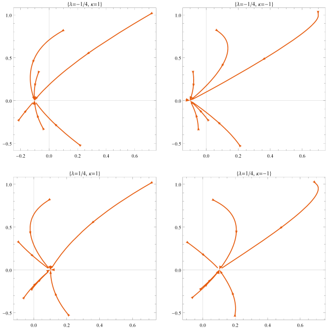
Figure 6: Phase space portrait in the space of variables $\left(x,z\right)$ for the dynamical system (18), (20) and for $\left(\varepsilon_{\phi},\varepsilon_{\psi}\right)=\left(-1,+1\right)$. The figures are for different values of the free parameters $\left\{\lambda,\kappa\right\}$. We observe that the unique attractor is point $P_{2}\left(B\right)$.

Figure 7: Qualitative evolution of $w_{eff}$ for the numerical solutions of the phase portraits in Fig. 6

IV.3.1 Analysis at infinity

As in the model B, parameters can take values at infinity. Thus we define the new coordinates

$$x=\frac{\cos u\cosh v}{\rho}~{},~{}y=\frac{\cos u\sinh v}{\rho}~{},~{}z=\frac{\sin u}{\rho}~{},$$ (27)

where the dynamical system becomes

$$\rho^{\prime}=\frac{1}{2}\left(\rho^{2}+1\right)\left(\kappa\rho\sqrt{3\left(1-\rho^{2}\right)}\cosh v-3\left(\rho^{2}-1\right)\sinh^{2}v\right)~{},$$ (28)

$$v^{\prime}=\frac{1}{4}\left(\sqrt{6}\left(\kappa+\lambda+\left(\kappa-\lambda\right)\rho^{2}\right)\frac{\sinh v}{\cos\left(\frac{1}{2}\arccos\left(-\frac{\rho^{2}}{2}\right)\right)}+6\rho\sinh\left(2v\right)\right)~{},$$ (29)

where $\rho^{2}+\cos\left(2\theta\right)=0$. We find only one stationary point at the infinity with coordinates $\left(\rho,v\right)$ to be $Q_{3}=\left(0,0\right)$. The point describes a solution in which only the kinetic parts of the scalar fields contribute to the cosmological fluid, while the eigenvalues of the linearized system are determined to be $e_{1}\left(Q_{3}\right)=\frac{\sqrt{3}}{2}\kappa,~{}e_{2}\left(Q_{3}\right)=\frac{\sqrt{3}}{2}\left(\kappa+\lambda\right)$, from where we infer that the point is an attractor when $\kappa<0$ and $\kappa<-\lambda$.

The phase portrait of the dynamical system (28), (29) is presented in Fig. 8.

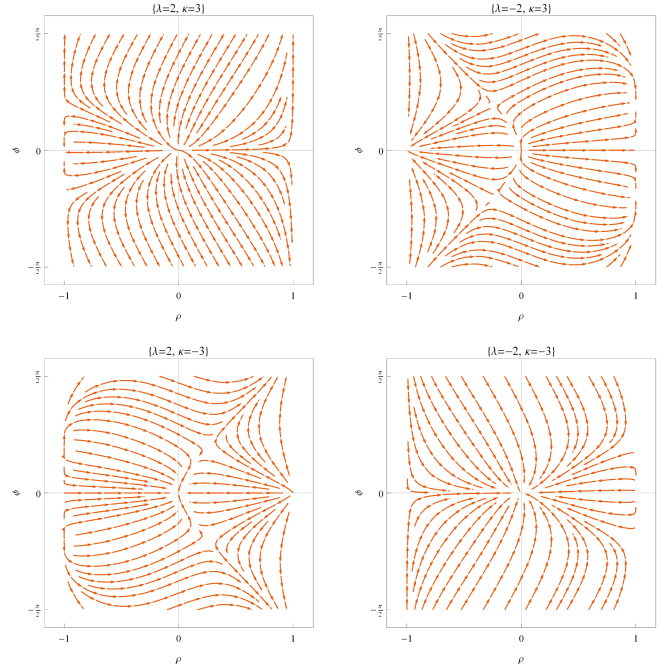
Figure 8: Phase space portrait in the space of variables $\left(\rho,v\right)$ for the dynamical system (28), (29). The figures are for different values of the free parameters $\left\{\lambda,\kappa\right\}$.

IV.4 Model D $\left(\varepsilon_{\phi},\varepsilon_{\psi}\right)=\left(-1,-1\right)$

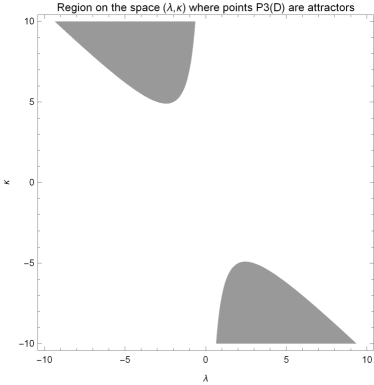
Figure 9: Region plots in the space of variables $\left(\lambda,\kappa\right)$ for which the stationary points $P_{3}^{\left(\pm\right)}\left(D\right)~{}$are attractors.

For the last case of our interest, where $\left(\varepsilon_{\phi},\varepsilon_{\psi}\right)=\left(-1,-1\right)$ the real stationary points are the $P_{2}\left(D\right)=\left(\frac{\lambda}{\sqrt{6}},\sqrt{1+\frac{\lambda^{2}}{6}},0\right)$ and $P_{3}^{\left(\pm\right)}\left(D\right)=\left(-\frac{\sqrt{6}}{\kappa+\lambda},\sqrt{\frac{\kappa}{\kappa+\lambda}},\pm\sqrt{-\frac{\lambda\left(\kappa+\lambda\right)+6}{\left(\kappa+\lambda\right)^{2}}}\right)$. Point $P_{2}\left(D\right)$ has same physical properties as $P_{2}\left(C\right)$, while points $P_{3}^{\left(\pm\right)}\left(D\right)$ have same physics as $P_{3}^{\left(\pm\right)}\left(C\right)$. Thus the stability properties change. Indeed the eigenvalues of the linearized system around the point $P_{2}\left(D\right)$  are $e_{1}\left(P_{2}\left(D\right)\right)=-3-\frac{\lambda^{2}}{2}~{},~{}e_{2}\left(P_{2}\left(D\right)\right)=\frac{1}{2}\left(-6-\lambda\left(\kappa+\lambda\right)\right)$ from which we infer that $P_{2}\left(D\right)$ is an attractor when $\left\{\lambda<0,\kappa<-\frac{6+\lambda^{2}}{\lambda}\right\}$ $\cup$ $\left\{\lambda>0,\kappa>-\frac{6+\lambda^{2}}{\lambda}\right\}\cup\left\{\kappa\in\mathbb{R},\lambda=0\right\}$. Stationary points $P_{3}^{\left(\pm\right)}\left(D\right)$ are physically acceptable when $\lambda\left(\kappa+\lambda\right)+6<0$, while the eigenvalues of the linearized system are determined to be $e_{\pm}\left(P_{3}^{\left(\pm\right)}\left(D\right)\right)=-\frac{3\kappa}{2\left(\kappa+\lambda\right)}\pm\frac{\sqrt{3\kappa}}{2\left(\kappa+\lambda\right)}\sqrt{\bar{\Delta}}$, with $\bar{\Delta}=4\lambda^{3}+8\kappa\lambda^{2}+\lambda\left(\kappa^{2}+6\right)+27\kappa$ from which we conclude that the exact scaling solutions at the stationary points are stable, i.e. points $P_{3}^{\left(\pm\right)}\left(D\right)$ are attractors when $\left\{\lambda<0,~{}\lambda\left(6+\lambda\left(\kappa+\lambda\right)\right)>0,\sqrt{48+\frac{729}{\lambda^{2}}}\leq 8\kappa+\frac{27}{\lambda+8\lambda}\right\}$ and  $\left\{\lambda>0,~{}\left(27+\lambda\left(8\kappa+\sqrt{48+\frac{729}{\lambda^{2}}}\right)\right)<0~{},-\frac{27}{8\lambda}-\lambda-\frac{1}{8}\sqrt{48+\frac{729}{{}^{\lambda^{2}}}}\leq\kappa<-\frac{6+\lambda^{2}}{\lambda}\right\}$ . The latter regions are plotted in Fig. 9. In Fig. 10 the phase portrait of the field equations in the space of variables $\left(x,z\right)$ is presented, while the qualitative evolution of the effective equation of state parameter is presented in Fig. 11. We observe that always $w_{eff}<-1$ and the $w_{eff}$ cannot cross the phantom divide line. Thus this model is not physically acceptable.

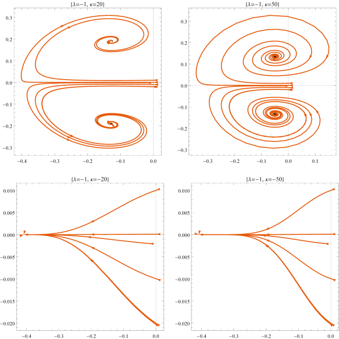
Figure 10: Phase space portrait in the space of variables $\left(x,z\right)$ for the dynamical system (18), (20) and for $\left(\varepsilon_{\phi},\varepsilon_{\psi}\right)=\left(-1,-1\right)$. The figures are for different values of the free parameters $\left\{\lambda,\kappa\right\}$.

Figure 11: Qualitative evolution of $w_{eff}$ for the numerical solutions of the phase portraits in Fig. 10

IV.4.1 Analysis at infinity

For mathematical completeness we proceed with the determination of stationary points at the infinity. In order to perform such an analysis we consider the new coordinates

$$x=\frac{\cos u\cos v}{\rho}~{},~{}y=\frac{\sin u}{\rho}~{},~{}z=\frac{\cos u\sin v}{\rho},$$ (30)

from where we find the equivalent dynamical system

$$\rho^{\prime}=\frac{1}{2}\left(1+\rho^{2}\right)\left(3\left(\rho^{2}-1\right)+\lambda\rho\sqrt{3\left(1-\rho^{2}\right)}\cos v\right)~{},~{}$$ (31)

$$v^{\prime}=\frac{\sqrt{3}}{2\sqrt{1-\rho^{2}}}\left(\kappa+\lambda+\rho^{2}\left(\lambda-\kappa\right)\right)\sin v~{},~{}$$ (32)

with equation of constraint $\rho^{2}+\cos\left(2u\right)=0$. The stationary points with $\rho=0$, are the points with $\sin v=0$. Thus, in the surface $\rho=0$, $\rho^{\prime}=\frac{3}{2}$, which means that the exact solutions at the points are sources.

V Conclusions

In this work we considered a two scalar field cosmological model for which the two scalar fields are minimally coupled to gravity, but they have an interaction term in the definition of their energy. Specifically, the dynamics of the two scalar fields evolves in a two-dimensional space of constant curvature. If the signature of the space is Euclidean and the scalar fields have positive kinetic energy, then our gravitational Action Integral takes the form of the Chiral model. However, in this analysis we considered the scalar fields to have also negative energy density. This leads to the requirement that the dynamics of the scalar fields evolve in a space of constant positive or negative curvature with Lorentzian or Euclidean signature

We performed a detailed analysis on the dynamics of this specific cosmological model in a spatially flat FLRW background space. In particular we determined the stationary points and we investigated their stability, in order to study the asymptotic behaviour of this cosmological theory and to understand the cosmological evolution as also to investigate the existence of cosmological solutions of special interest. For the completeness of our study we investigated four different cases, which we called them models A, B, C and D.

Model A corresponds to the Chiral model, in which the two scalar fields have positive kinetic energy. We found that the gravitational field equations admit three different kinds of exact solutions which correspond to the two scaling solutions of the quintessence (one scalar field model) while the third solution is also a scaling solution wherein the two scalar fields contribute to the cosmological evolution. The effective parameter for the equation of state has lower bound at $-1,$ that is $w_{eff}\left(A\right)>-1$.

For model B, the second scalar field has a negative kinetic energy and can be seen as the generalization of the quintom theory. Indeed, the quintom model is recovered when the coupling parameter of the two scalar fields becomes zero. The number of the stationary points are exactly the same as for Model A. Thus in this case the parameter for the equation of state for the effective fluid can cross the phantom divide lines, twice, which means that it can start from a value larger than $-1$, then become smaller than $-1$ and at the end to reach again a value larger than $-1$. That is exactly similar to the behaviour of the equation of state parameter for the quintom model. It is important to mention that in our numerical simulation we have not seen the appearance of ghosts. Hence, that makes this specific case of special interest for further investigation.

Models C and D admit only two different sets of scaling solutions in the finite region, while only model C admits an additional point at infinity. For model C the equation of state parameter can cross the phantom divide line only one time, but for model D the equation of state parameter is always lower than $-1$, which means that the model D is not of physical interest.

From the above analysis we conclude that model B, which can be seen as a generalization of the quintom model can describe some of the recent observations and deserves further attention. In a forthcoming work we will investigate the existence of additional exact and solutions for this specific model.

- (1) M. Tegmark et al., Astrophys. J. 606, 702 (2004)
- (2) D. N. Spergel et al., Astrophys. J. Supplt. 170, 377 (2007)
- (3) T. M. Davis et al., Astrophys. J. 666, 716 (2007)
- (4) M. Kowalski et al., Astrophys. J. 686, 749(2008)
- (5) G. Hinshaw et al., Astrophys. J. Supplt. 180, 225 (2009)
- (6) J. A. S. Lima and J. S. Alcaniz, Mon. Not. Roy. Astron. Soc. 317, 893 (2000)
- (7) J. F. Jesus and J. V. Cunha, Astrophys. J. Lett. 690, L85 (2009)
- (8) S. Basilakos and M. Plionis, Astrophys. J. Lett. 714, 185 (2010)
- (9) E. Komatsu E. et al., 2011, Astrophys. J. Sup., 192, 18 (2011)
- (10) O. Farooq, D. Mania and B. Ratra, Astrophys. J., 764, 138 (2013)
- (11) P. A. R. Ade et al., (Planck Collaboration), Astronomy and Astrophysics 571, A16 (2014)
- (12) N. Aghanim et al., (Planck Collaboration), Astronomy and Astrophysics 641, A6 (2020)
- (13) A. Guth, Phys. Rev. D 23, 347 (1981).
- (14) A. Linde, Phys. Lett. B 108, 389 (1982).
- (15) E. J. Copeland, M. Sami and S. Tsujikawa, Int. J. Mod. Phys. D 15, 1753 (2006).
- (16) T. Clifton, P.G. Ferreira, A. Padilla and C. Skordis, Phys. Rept. 513, 1 (2012)
- (17) S. Nojiri, S. D. Odintsov and V. K. Oikonomou, Phys. Rept. 692, 1 (2017)
- (18) E. J. Copeland, M. Sami and S. Tsujikawa, Intern. Journal of Modern Physics D 15, 1753, (2006)
- (19) L. Amendola and S. Tsujikawa, Dark Energy Theory and Observations, Cambridge University Press, Cambridge UK, (2010)
- (20) B. Ratra and P.J.E. Peebles, Phys. Rev. D 37, 3406 (1988)
- (21) T. Harko, F.S.N. Lobo and M.K. Mak, EPJC 74, 2784 (2014)
- (22) C. Rubano and J. D. Barrow, Phys. Rev. D. 64, 127301 (2001)
- (23) L. A. Urena-Lopez, T. Matos, Phys. Rev. D 62, 081302 (2000)
- (24) V. Sahni and A. Starobinsky, Int. J. Mod. Phys. D 9 373 (2000)
- (25) A. Paliathanasis, M. Tsamparlis, S. Basilakos and J.D. Barrow, Phys. Rev. D 91, 123535 (2015)
- (26) N. Dimakis, A. Karagiorgos, A. Zampeli, A. Paliathanasis, T. Christodoulakis and P.A. Terzis, Phys. Rev. D 93, 123518 (2016)
- (27) W. Fang, H.Q. Lu, Z.G. Huang and K.F. Zhang, Int. J. Mod. Phys. D 15, 199 (2006)
- (28) M. Cataldo, F. Arevalo and P. Mella, Astr. Sp. Sci. 344, 495 (2013)
- (29) S. Nojiri, S.D. Odintsov, V.K. Oikonomou and E.N. Saridakis, JCAP 09, 044 (2015)
- (30) Y.F. Cai, E.N. Saridakis, M.R. Setare and J.-Q. Xia, Phys. Rep. 493, 1 (2010)
- (31) M.R. Setare and E.N. Saridakis, Int. J. Mod. Phys. D 18, 549 (2009)
- (32) R. Lazkoz, G. Leon and I. Quiros, Phys. Lett. B 649, 103 (2007)
- (33) G. Leon, A. Paliathanasis and J.L. Morales-Martinez, Eur. Phys. J. C 78, 753 (2018)
- (34) E. Elizalde, S. Nojiri, S.D. Odintsov, D. Saez-Gomez and V. Faraoni, Phys. Rev. D 77, 106005 (2008)
- (35) W. Yang, M. Shahalam, B. Pal, S. Pan and A. Wang, Constraints on quintessence scalar field models using cosmological observations, to appear in Phys. Rev. D [arXiv:1810.08586]
- (36) S.V. Chervon, Quantum Matter 2, 71 (2013)
- (37) P. Christodoulidis, D. Roest, E.I. Sfakianakis, JCAP 11, 012 (2019)
- (38) A. Beesham, S.V. Chernov, S.D. Maharaj and A.S. Kubasov, Quantum Matter 2, 388 (2013)
- (39) R.R. Abbyazov and S.V. Chernov, Grav. Cosmol. 18, 262 (2012)
- (40) R.J. Scherrer, Phys. Rev. Lett. 93, 011301 (2004)
- (41) A. Bandyopadhyay, D. Gangopadhyay and A. Moulik, EPJC 72, 1943 (2012)
- (42) C. Armendariz-Picon, T. Damour, V. Mukhanov, Phys. Lett. B 458, 209 (1999)
- (43) T. Damouri and G. Espsito-Farese, Class. Quant. Grav. 9, 2093 (1992)
- (44) G.W. Hordenski, Int. J. Theor. Phys. 10, 363 (1975)
- (45) C. Deffayet, G. Esposito-Farese and A. Vikman, Phys. Rev. D 79, 084003 (2009)
- (46) A.A. Coley and R.J. van den Hoogen, Phys. Rev. D 62, 023517 (2000)
- (47) T.P. Sotiriou, In Papantonopoulos E. (eds) Modifications of Einstein’s Theory of Gravity at Large Distances, Lecture Notes in Physics, vol 892. Springer, Cham (2014)
- (48) A. Paliathanasis and M. Tsamparlis, Phys. Rev. D 90, 043529 (2014)
- (49) A. Paliathanasis, Class. Quantum Grav. 37, 195014 (2020)
- (50) N. Dimakis, A. Paliathanasis, P.A. Terzis and T. Christodoulakis, EPJC 79, 618 (2019)
- (51) N. Dimakis and A. Paliathanasis, Crossing the phantom divide line as an effect of quantum transitions, (2020) [arXiv:2001.09687]
- (52) E.J. Copeland, A.R. Liddle and D. Wands, Phys. Rev. D 57, 4686 (1998)
- (53) G. Leon and E.N. Saridakis, JCAP 04, 031 (2015)
- (54) G. Leon and E.N. Saridakis, JCAP 11, 006 (2009)
- (55) R. Lazkoz and G. Leon, Phys. Rev. D 71, 123516 (2005)
- (56) L. Amendola, R. Gannouji, D. Polarski and S. Tsujikawa, Phys. Rev. D 95, 083504 (2007)
- (57) L. Amendola, D. Polarski and S. Tsujikawa, Phys. Rev. Lett. 98, 131302 (2007)
- (58) A. Giacomini, S. Jamal, G. Leon, A. Paliathanasis and J. Saveedra, Phys. Rev. D 95, 124060 (2017)
- (59) G. Leon, A. Paliathanasis and J.L. Morales-Martinez, EPJC 78, 753 (2018)
- (60) W. Yang, S. Pan, E. Di Valentino, R.C. Nunes, S. Vagnozzi and D.F. Mota, JCAP 18, 019 (2019)
- (61) W. Yang, S. Pan and A. Paliathanasis, MNRAS 482, 1007 (2019)
- (62) W. Yang, N. Banarjee, A. Paliathanasis and S. Pan, Phys. Dark Energy 26, 100383 (2019)
- (63) W. Yang, A. Mukherjee, E. Di Valentino and S. Pan, Phys. Rev. D 98, 123527 (2018)
- (64) S. Pan and G.S. Sharov, MNRAS 472, 4736 (2017)
- (65) W. Yang, S. Pan, E. Di Valentino, B. Wang and A. Wang, JCAP 20, 050 (2020)