RAR-U-NET: a Residual Encoder to Attention Decoder by Residual Connections Framework for Spine Segmentation under Noisy Labels

Abstract

Segmentation algorithms for medical images are widely studied for various clinical and research purposes. In this paper, we propose a new and efficient method for medical image segmentation under noisy labels. The method operates under a deep learning paradigm, incorporating four novel contributions. Firstly, a residual interconnection is explored in different scale encoders to transfer gradient information efficiently. Secondly, four copy-and-crop connections are replaced by residual-block-based concatenation to alleviate the disparity between encoders and decoders. Thirdly, convolutional attention modules for feature refinement are studied on all scale decoders. Finally, an adaptive denoising learning strategy (ADL) is introduced into the training process to avoid too much influence from the noisy labels. Experimental results are illustrated on a publicly available benchmark database of spine CTs. Our proposed method achieves competitive performance against other state-of-the-art methods over a variety of different evaluation measures.

Index Terms—  Semantic Segmentation, Computed Tomography, Spine, Noisy Label

1 Introduction

The encoder-decoder model has been one of the most prominent deep neural network architectures used in medical image segmentation. U-Net [1] is a completely symmetric variety of encoder-decoder. The encoder extracts pixel location features via down sampling; and the decoder recovers the spatial dimension and pixel location information with a deconvolution operation. Between the encoder and decoder layer, there is a copy-and-crop connection to deliver multi-scale information. U-Net has been used successfully for segmentation a variety of areas in the human body. In 2016, Ronneberger proposed a 3D U-Net which carried out volumetric segmentation through extracting sparsely annotated volumetric images [2]. This is achieved at the cost of an increase in the number of training parameters. In 2018 Oktay [3] proposed an attention gate model to enable convolutional neural networks automatically to learn target structures of different shapes and sizes. It is based on Attention U-Net which achieves higher sensitivity and accuracy while requiring minimal computational overhead. In 2019, Residual Networks, Inception Networks, Densely Connected Networks and several modified U-Net have continued to be explored and optimised [4, 5, 6]. The high resolution Dense-U-Net Network for spine segmentation proposed by Kolařík et al. [7] explores the performance of 2D and 3D U-Nets in residual networks and densely connected networks. Due to the 3D convolutional layers and interconnections, this architecture is costly in training parameter time.

Meanwhile, a separate hurdle when segmenting medical data is the potential lack of precision in the annotated contours, usually due to limitations in knowledge and to clinicians’ subjectivity. Results of the annotation process can depart from the the gold standard: labelled features can present slight erosion or dilation of what would be the ideal contours, as well as various kinds of elastic transformations. We hereafter call such variations ‘noisy labels’, which will affect the effect of the final model.

In this work, we overcome the shortcomings described above through RAR-U-Net, a Residual encoder to Attention decoder by Residual connections framework for medical image segmentation under noisy labels. Its main novelty consists of:

1) shortcut interconnections on the four down-sampling blocks as residual encoders, to enhance gradient information transfer,

2) residual-block-based concatenation to mitigate the disparity between encoders and decoders,

3) convolutional attention module on four up-sampling blocks to capture essential information,

4) adaptive denoising learning strategy which eliminates the negative effects of noise labels in the training process.

2 Methods

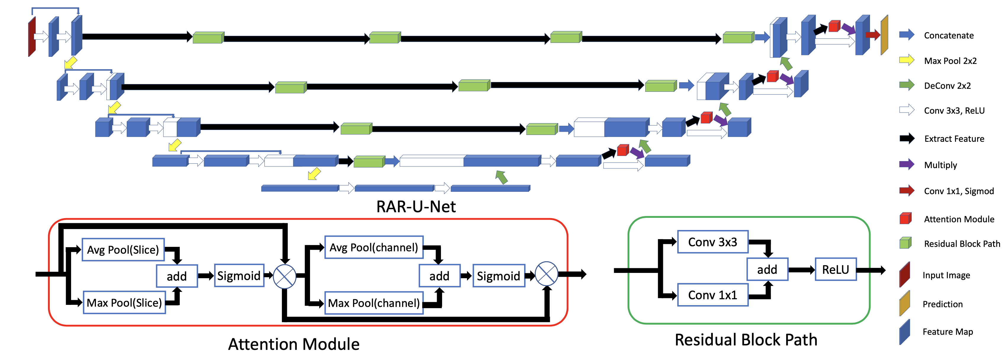
Fig. 1: The Architecture of the Proposed Network, Attention Module and Residual Block Path

The architecture of RAR-U-Net is illustrated in Fig. 1. It is a symmetrical architecture which consists of convolution, upsampling and downsampling, allowing to contract and recover pixel-level information. We detail below the four specific contributions of this method.

2.1 Residual Interconnections Networks

Inspired by ResNet [8], a concatenation function is allocated to each down-sampling block. In order to strengthen the ability to express features and gradient information, after obtaining the downsampled features of a previous layer, these features will go through a new feature extraction process. The extraction process consists of the repeated application of two $3\times 3$ unpadded convolutions, each followed by a rectified linear unit (ReLU). The number of feature channels is doubled compared to the previous layer after the first $3\times 3$ convolution operator. Finally, we concatenate the downsampled feature with the feature acquired from the second $3\times 3$ convolution operator. This operation aims to establish connections between different layers, making full use of feature information and alleviating the gradient disappearance problem.

2.2 Residual-Block-Based Concatenation

To mitigate the disparity between encoders and decoders which may degrade the segmentation performance [9], the four copy and crop connections are replaced by residual-block-based concatenation. We adopt residual learning to connect the encoder to the decoder in each layer.

We define the Residual Block Path as a building block of our model, also sketched in Fig. 1. Formally, if $x$ and $y$ are the input and output vectors of the layers, then

$$y=F(x,\left\{{W_{i}}\right\})+x$$ (1)

where the Eq. 1 illustrates residual block, and $F(x,\left\{{W_{i}}\right\})$ represents the residual mapping to be learned. For example in Fig. 1 that has one $3\times 3$ layer, $F=\sigma{W_{1}}x$ in which $\sigma$ and $W$ denote the ReLU activation and weight, to simplify notation, the biases are omitted. The operation $F+x$ is performed by a shortcut connection and element-wise addition. We also use a $1\times 1$ convolution operator to match the number of channels. After the addition operation we adopt the second non-linearity ReLU. Finally, the feature map processed through the residual block is concatenated with the upsampled feature of the decoder. To mitigate the difference between each level of the encoder and decoder, and considering the computational cost, the number of Residual Blocks at each level of the encoder-decoder is set to 4, 3, 2 and 1, respectively.

2.3 Convolutional Attention Module

To enhance the performance of the decoder classification for each pixel by capturing essential information in the presence of noisy labels, we explore the use of an attention mechanism. Unlike attention gate filter features from skip connections [3], an attention module can normally be integrated with convolutional layers to enhance key information of the feature map with pooling layers and sigmoid activation functions [10].

Our proposed attention module for the convolutional layer of decoder is sketched in Fig. 1. There are two parts of the attention module related to the channel– and spatial attention of different feature maps. Both parts are developed by the pooling layer and sigmoid activation. Average and max pooling layers avoid noisy label gradients to keep trunk parameters. The sigmoid function simultaneously generates a weight attention value as output for each pixel location and channel.

Fig. 1 shows how a feature map $F\in R^{W\times H\times C}$ with the size of shape $W\times H\times C$ from a previous CNN is sent to the attention module pipeline. The feature maps from the average pooling layers and max pooling layers of spatial dimensions $W\times H$ are denoted $F^{Avg}_{Spatial}$ and $F^{Max}_{Spatial}\in R^{W\times H\times 1}$. Similarly, $F^{Avg}_{Channel}$ and $F^{Max}_{Channel}\in R^{1\times 1\times C}$ are the feature maps from average pooling layers and max pooling layers on the channel dimension $C$.

Both of the spatial attention value ${W_{Spa}}$ and channel attention value ${W_{Channel}}$ are calculated through the sigmoid activation $\sigma$. The final output feature map $F_{out}$ is adaptively refined from feature map $F$ through a spatial attention layer and channel attention layer successively, in order to capture essential information.

$$\small W_{Spa}=\sigma(F^{Avg}_{Spa}+F^{Max}_{Spa})$$ (2)

$$\small W_{Channel}=\sigma(F^{Avg}_{Channel}+F^{Max}_{Channel})$$ (3)

$$\small F_{out}=W_{Channel}(W_{Spa}(F)\otimes F)\otimes(W_{Spa}(F)\otimes F)$$ (4)

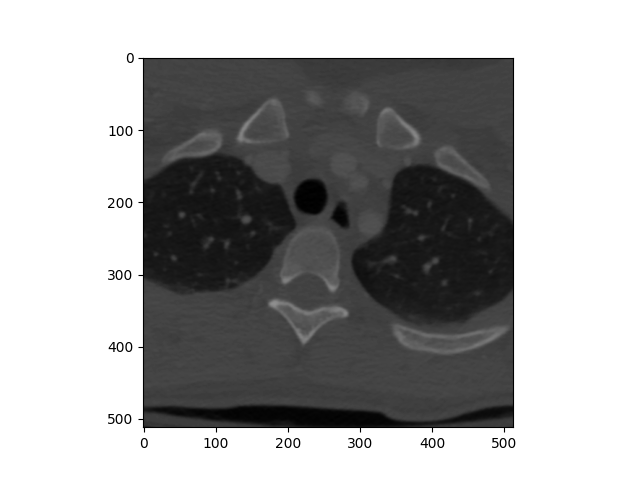
(a) Raw image

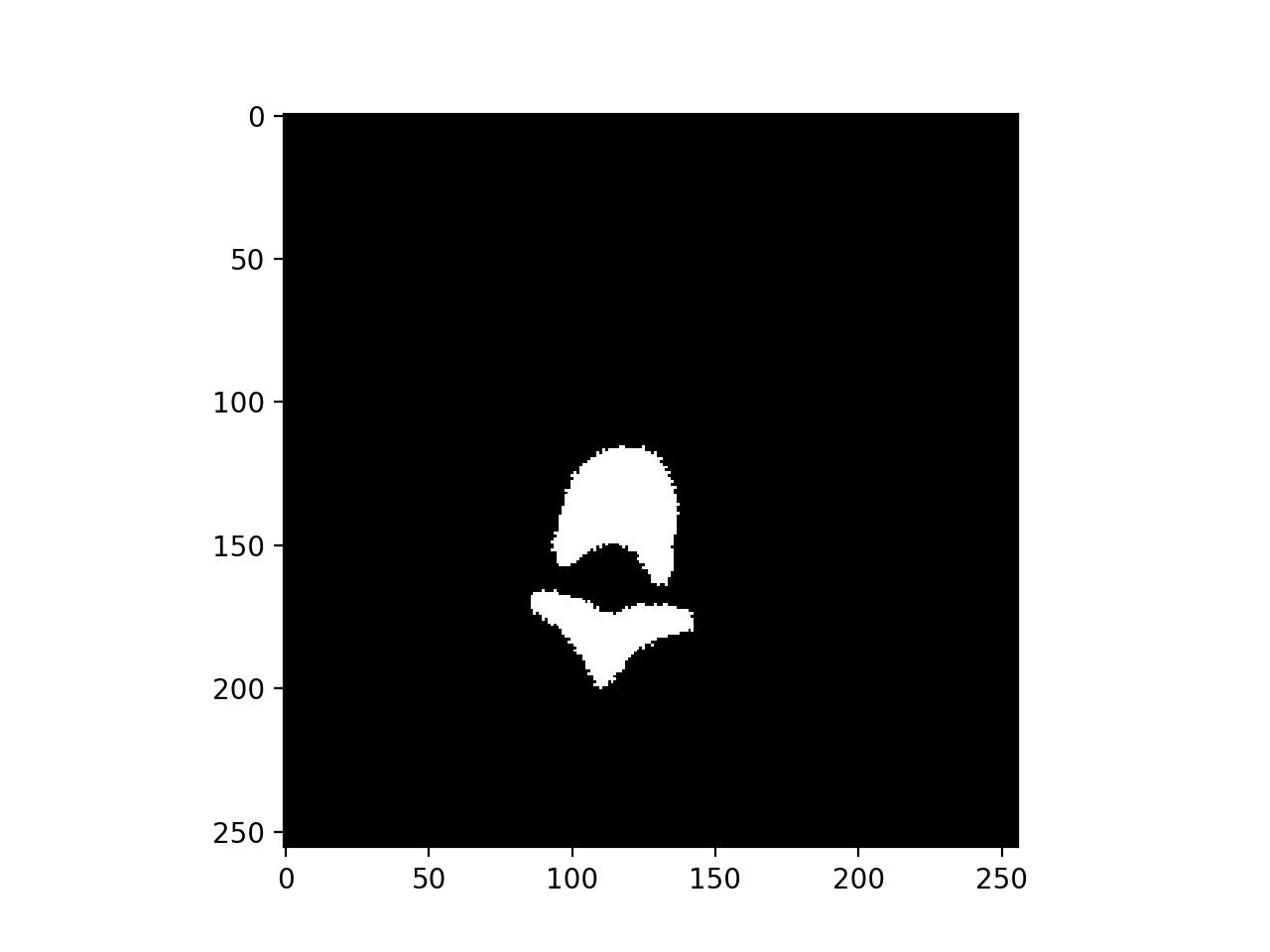
(b) GT mask

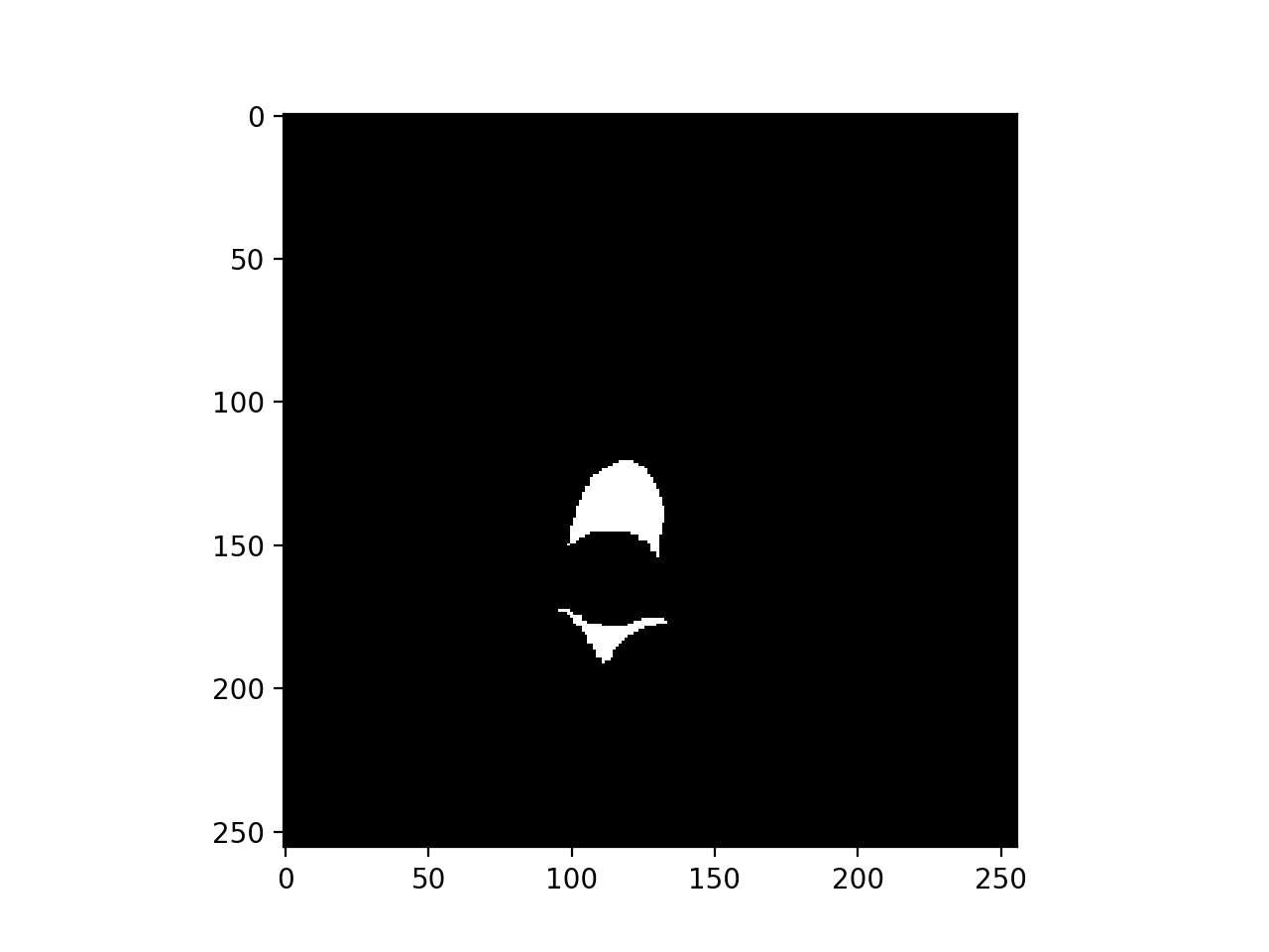
(c) Erosion

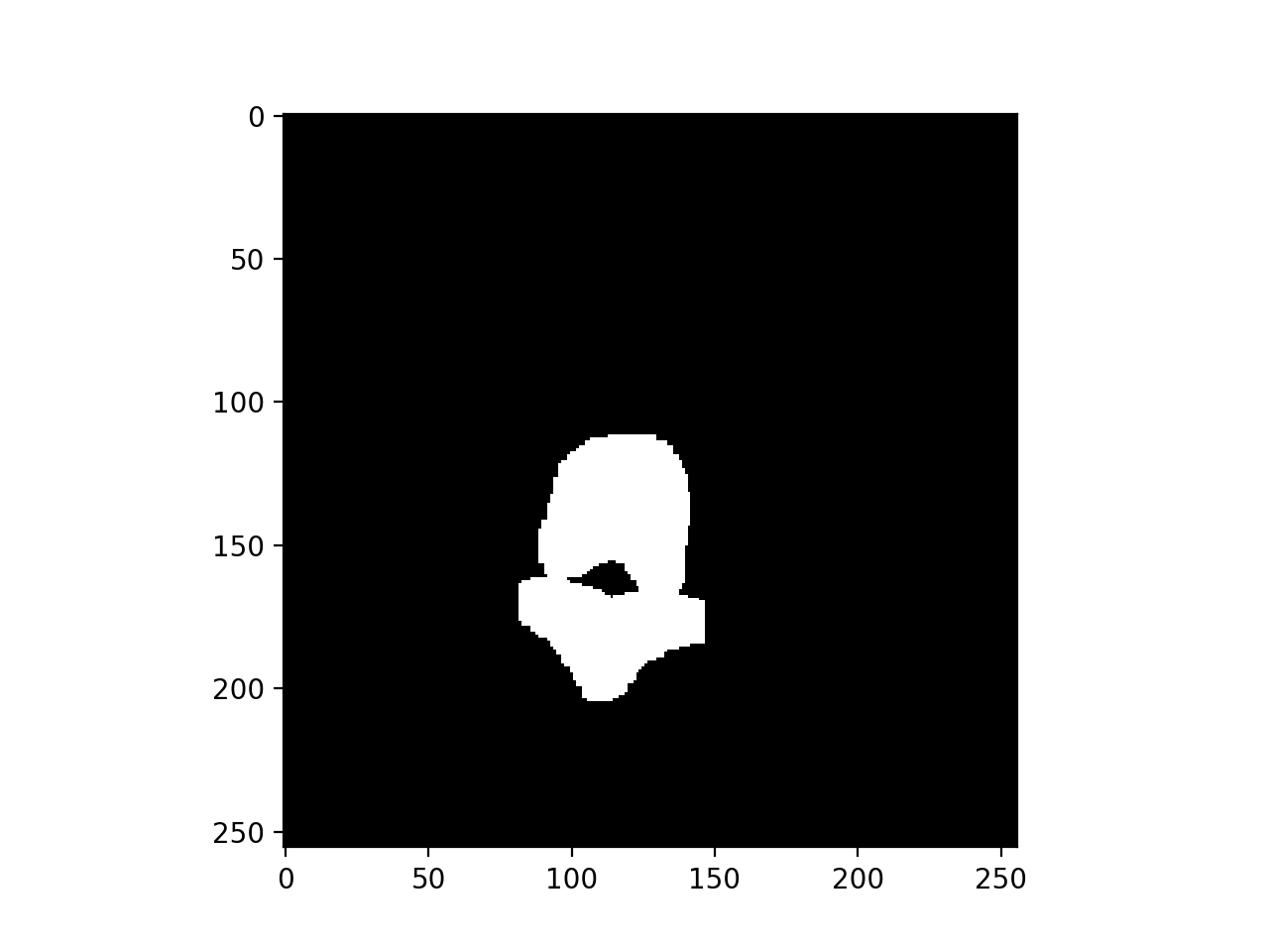
(d) Dilation

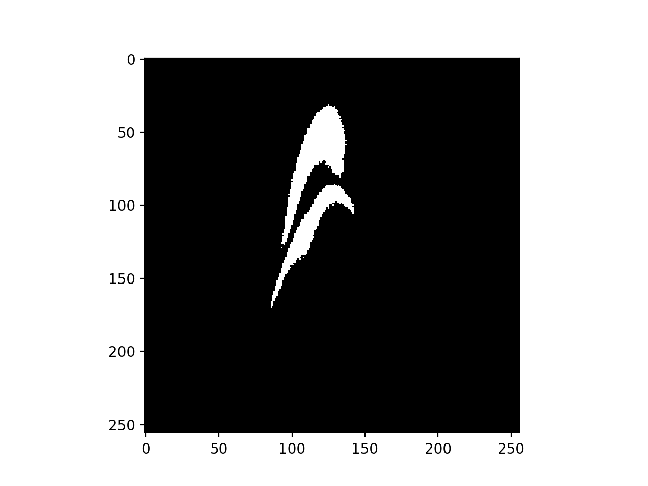
(e) Elastic transform

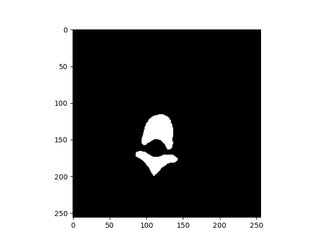
(f) Predicted result

Fig. 2: Examples of Spine CT Slice and its Alterations

2.4 Adaptive Denoising Learning

In order to simulate the challenge of noisy (or inaccurate) labels emerging from practical settings, we propose a strategy of adaptive denoising to be applied during the training process. To simulate this situation, a certain proportion $\beta$ of masks in the training data have been replaced with synthetically generated noisy labels. These labels present with erosions, dilations or elastic transforms. The extent of the noise present is denoted by $\alpha\in[0,1]$. Three such examples are illustrated in Fig. 2(c)–2(e), which are noisy in some sense compared to the ground truth in Fig. 2(b). The noise level $\alpha$ can be thought of as the extent of the overlap between the original ground truth mask and the generated noisy label.

We propose a simple and efficient adaptive denoising learning strategy. Inspired by O2U-Net [11], the difference between each prediction and label data is calculated and recorded at every training epoch. The higher the loss of a label, the higher its probability of being a noisy label. During training, our strategy aims to detect and remove a number of high loss value labels. A large number of noisy labels get detected at the begining of the training iteration, and then a few more towards the end. This is because the training process evolves from underfitting to overfitting. The number $N(t)$ of labels detected and removed in each epoch is

$$N(t)=\left\{\begin{array}[]{lr}0.5(1-\alpha)\beta y,&0<t<0.1(1-\alpha)\beta x\\ \frac{-y}{x}t+0.6(1-\alpha)\beta y,&0.1(1-\alpha)\beta x\leq t\\ &\&~{}~{}t\leq 0.5(1-\alpha)\beta x\\ 0.1(1-\alpha)\beta y,&0.5(1-\alpha)\beta x<t\leq x\end{array}\right.$$ (5)

where $t$ is the current training epoch, $\alpha$ is the noise level, $\beta$ is the proportion of items in the training dataset to which noise has been applied, $x$ is the total number of training epochs, and $y$ is the total number of masks. 0.1 and 0.5 are hyperparameters obtained using a systematic search.

3 Experiments and Results

Table 1: Direct Comparison Against Existing Algorithms

Model	Dice	Acc	Pre	Rec	Spe	Par $10^{6}$
UNet	0.8360	0.9863	0.8832	0.7936	0.9952	7.26
Residual-UNet	0.8810	0.9898	0.9097	0.8540	0.9961	9.90
Densely-UNet	0.8316	0.9860	0.8832	0.7857	0.9952	15.47
M-UNet	0.9478	0.9954	0.9512	0.9444	0.9978	7.77
M-Densely-UNet	0.9517	0.9958	0.9524	0.9508	0.9978	15.48
VGG16 UNet	0.9138	0.9925	0.9235	0.9043	0.9966	23.75
VGG19 UNet	0.9024	0.9914	0.9029	0.9019	0.9955	29.06
ResNet34 UNet	0.6626	0.9689	0.6333	0.6947	0.9815	24.45
SE-ResNet34 UNet	0.7306	0.9762	0.7265	0.7347	0.9873	24.61
ResNeXt101 UNet	0.7597	0.9765	0.6909	0.8438	0.9826	32.06
DenseNet121 UNet	0.7982	0.9811	0.7526	0.8498	0.9872	12.13
InceptionV3 UNet	0.8109	0.9837	0.8250	0.7972	0.9922	29.93
EfficientNet UNet	0.8358	0.9857	0.8431	0.8286	0.9929	10.11
MultiRes UNet	0.8542	0.9864	0.8094	0.9043	0.9902	7.76
3D UNet	0.8078	0.9874	0.7788	0.8390	0.9922	22.58
3D Residual-UNet	0.7757	0.9850	0.7360	0.8198	0.9904	28.15
3D Densely-UNet	0.7921	0.9860	0.7450	0.8456	0.9906	44.78
3D Attention UNet	0.8623	0.9870	0.8129	0.9182	0.9902	22.60
LinkNet	0.8958	0.9908	0.8919	0.8999	0.9950	20.32
FPN	0.8804	0.9893	0.8675	0.8936	0.9937	17.59
RAR-U-Net	0.9580	0.9963	0.9605	0.9554	0.9982	11.79

3.1 Dataset and Experimental Setup

We used a publicly available spine dataset from California and NIH [12], which consists of CT scans from 10 patients, of up to 600 slices per scan, at a resolution of $512\times 512$, and $1$mm inter-slice spacing. All images are normalized and resized to $256\times 256$. Ground truth (GT) masks are available for each image, some of which were used as input for the noise introduction. Data augmentation was applied in the form of $\pm 90^{\circ}$ rotations. Of the 10 scans, 9 were used for training and 1 for testing. Validation is carried out on 10% of the training data. An overlapping approach allowing to add eight more surrounding slices in each training batch is utilized to ensure the 3D model collect continuous information.

Table 2: Difference Measures of the Segmentation Results

	HD (pixels)	ASSD (pixels)	RVD $\in[0,1]$
RAR-U-Net	10.0110	0.8221	0.0518

Table 3: Boundary-based Match in the Segmentation Results

	DBDG	DBDM	SBD
RAR-U-Net	0.8425	0.8564	0.8465

Table 4: Ablation Studies on Contributions of Architecture

Residual Encoders	Residual Connections	Attention Decoders	IOU	Recall	Trainable Parameters
			0.7182	0.8832	7,762,465
✓			0.7873	0.8540	9,899,625
	✓		0.9119	0.9549	8,912,673
		✓	0.8927	0.9406	7,785,157
✓		✓	0.9070	0.9481	9,922,317
✓	✓		0.9126	0.9535	11,049,833
✓	✓	✓	0.9193	0.9605	11,794,125

Table 5: Ablation Studies on ADL

Proportion	Level	Algorithm	ADL	IOU	Recall
75%	0.68	U-Net		0.6445	0.7303
75%	0.68	U-Net	✓	0.6742	0.8072
75%	0.68	Residual-UNet		0.7732	0.9097
75%	0.68	Residual-UNet	✓	0.8138	0.9462
75%	0.68	Attention-UNet		0.7809	0.8823
75%	0.68	Attention-UNet	✓	0.8087	0.9142
50%	0.77	UNet		0.7523	0.8420
50%	0.77	UNet	✓	0.8522	0.9295
50%	0.77	Attention-UNet		0.8464	0.9201
50%	0.77	Attention-UNet	✓	0.8561	0.9283
25%	0.85	Residual-UNet		0.8615	0.9051
25%	0.85	Residual-UNett	✓	0.8868	0.9433
25%	0.85	Dense-UNet		0.8443	0.9378
25%	0.85	Dense-UNett	✓	0.8864	0.9424
25%	0.55	U-Net		0.8024	0.8698
25%	0.55	U-Net	✓	0.8304	0.9176
25%	0.55	Residual-UNet		0.8230	0.8956
25%	0.55	Residual-UNet	✓	0.8495	0.9126

The RAR-U-Net code was developed in Python using Tensorflow [13]. It has been run on an Nvidia GeForce RTX2080 Ti GPU with 16GB memory, and Intel(R) Xeon(R) CPU E5-2650 v4. The runtimes varied between 1000–1200 mins for 50 epochs, including the data transfer. With a training batch size of 8, the learning rate is $10^{-5}$. The loss function is based on the Dice coefficient.

3.2 Results and Discussion

Figs. 2(a), 2(b), and 2(f) illustrate examples of a raw image, GT mask and average predicted result. RAR-U-Net is compared with classical segmentation algorithms including LinkNet [14], FPN [15], 3D UNet [2], MultiResUnet [9], DenselyUnet [7], and U-Net with classical backbones such as VGG [16], ResNet[8], SE-ResNet [17], ResNeXt [18], InceptionV3 [19] and EfficientNet [20]. We first compare the performance of our algorithm against a collection of widely used overlap measures such as the Dice coefficient, Accuracy, Precision, Sensitivity (or Recall), Specificity, which enable the comparison against other methods. These are illustrated in Table 1, together with the number of training parameters. The proportion of noisy labels in this case is 0.

The performance of our algorithm through difference measures such as the Hausdorff Distance, Average Symmetric Surface Distance (ASSD) and Relative Volume Difference (RVD) is shown in Table 2 – the smaller, the better.

Table 3 reports the extent to which the boundaries of the machine segmentation MS match those of the GT [21], using the Directed Boundary Dice relative to GT (DBD_G), Directed Boundary Dice relative to MS (DBD_M) and Symmetric Boundary Dice (SBD). In a von Neumann neighbourhood $N_{x}$ of each pixel $x$ on the boundary $\partial G$ of the ground truth,

$$\small DBD_{G}=DBD(G,M)=\displaystyle\frac{\rule{0.0pt}{11.62495pt}\sum\limits_{x\in\partial G}\text{Dice}(N_{x})}{\left|\partial G\right|}$$ (6)

$$\small SBD=\displaystyle\frac{\rule{0.0pt}{11.62495pt}\sum\limits_{x\in\partial G}DSC(N_{x})+\sum\limits_{y\in\partial M}DSC(N_{y})}{\left|\partial G\right|+\left|\partial M\right|}$$ (7)

These measures penalise mislabelled areas in the machine segmentation. Even a 75% close match between the boundaries is considered a good result.

3.3 Ablation study

In order to analyze the effects of each of the four proposed contributions and their combinations, extensive ablation experiments have been conducted. Table 4 documents how the removal of one or more components compromises the overall performance. The same table also gives a measure of the complexity of the overall RAR-U-Net model and its sub models. Table 5 focuses specifically on the effect of the ADL strategy. ‘Proportion’ and ‘Level’ illustrate how many images are randomly chosen to be processed as a noisy label and their level of noise in the training dataset. These have been varied more than shown here. ‘Algorithm’ illustrates that different algorithms are separately utilized for training; the adaptive denoising level ‘ADL’ strategy enables all models to perform better under noisy labels.

4 Conclusions

Our experimental results demonstrate that all four proposed contributions significantly improve segmentation under noisy labels, at a smaller training parameter cost. Although the tests were specific to a single public dataset, the methods are generic.

References

- [1] O Ronneberger et al., “U-Net: Convolutional networks for biomedical image segmentation,” in Int Conf Med Im Comp & Comp-Assisted Intervention. Springer, 2015, pp. 234–241.
- [2] Özgün Çiçek, Ahmed Abdulkadir, Soeren S Lienkamp, Thomas Brox, and Olaf Ronneberger, “3D U-Net: learning dense volumetric segmentation from sparse annotation,” in Int Conf Med Im Comp & Comp-Assisted Intervention. Springer, 2016, pp. 424–432.
- [3] O Oktay et al., “Attention U-Net: Learning where to look for the pancreas,” Int Conf Medical Imaging with Deep Learning, 2018.
- [4] Steven Guan, Amir A Khan, Siddhartha Sikdar, and Parag V Chitnis, “Fully dense unet for 2-d sparse photoacoustic tomography artifact removal,” IEEE journal of biomedical and health informatics, vol. 24, no. 2, pp. 568–576, 2019.
- [5] Foivos I Diakogiannis, François Waldner, Peter Caccetta, and Chen Wu, “Resunet-a: a deep learning framework for semantic segmentation of remotely sensed data,” ISPRS Journal of Photogrammetry and Remote Sensing, vol. 162, pp. 94–114, 2020.
- [6] Zongwei Zhou, Md Mahfuzur Rahman Siddiquee, Nima Tajbakhsh, and Jianming Liang, “Unet++: A nested u-net architecture for medical image segmentation,” in Deep Learning in Medical Image Analysis and Multimodal Learning for Clinical Decision Support, pp. 3–11. Springer, 2018.
- [7] M Kolařík et al, “Optimized high resolution 3d dense-u-net network for brain and spine segmentation,” Applied Sciences, vol. 9, no. 3, pp. 404, 2019.
- [8] K He et al, “Deep residual learning for image recognition,” in Proc IEEE CVPR, 2016, pp. 770–778.
- [9] Nabil Ibtehaz and M Sohel Rahman, “Multiresunet: Rethinking the u-net architecture for multimodal biomedical image segmentation,” Neural Networks, vol. 121, pp. 74–87, 2020.
- [10] S Woo et al., “CBAM: Convolutional block attention module,” in Proc ECCV, 2018, pp. 3–19.
- [11] J Huang et al., “O2U-Net: A simple noisy label detection approach for deep neural networks,” in Proc IEEE ICCV, 2019, pp. 3326–3334.
- [12] J Yao et al, “Detection of vertebral body fractures based on cortical shell unwrapping,” in Int Conf Med Im Comp & Comp-Assisted Intervention. Springer, 2012, pp. 509–516.
- [13] Martín Abadi and etc, “TensorFlow: Large-scale machine learning on heterogeneous systems,” 2015, Software available from tensorflow.org.
- [14] Abhishek Chaurasia and Eugenio Culurciello, “Linknet: Exploiting encoder representations for efficient semantic segmentation,” in 2017 IEEE Visual Communications and Image Processing (VCIP). IEEE, 2017, pp. 1–4.
- [15] Seung-Wook Kim, Hyong-Keun Kook, Jee-Young Sun, Mun-Cheon Kang, and Sung-Jea Ko, “Parallel feature pyramid network for object detection,” in Proceedings of the European Conference on Computer Vision (ECCV), 2018, pp. 234–250.
- [16] Karen Simonyan and Andrew Zisserman, “Very deep convolutional networks for large-scale image recognition,” Int Conf Learning Representations(ICLR), 2015.
- [17] Jie Hu, Li Shen, and Gang Sun, “Squeeze-and-excitation networks,” in Proceedings of the IEEE conference on computer vision and pattern recognition, 2018, pp. 7132–7141.
- [18] Saining Xie, Ross Girshick, Piotr Dollár, Zhuowen Tu, and Kaiming He, “Aggregated residual transformations for deep neural networks,” in Proceedings of the IEEE conference on computer vision and pattern recognition, 2017, pp. 1492–1500.
- [19] Christian Szegedy, Vincent Vanhoucke, Sergey Ioffe, Jon Shlens, and Zbigniew Wojna, “Rethinking the inception architecture for computer vision,” in Proc IEEE CVPR, 2016, pp. 2818–2826.
- [20] Mingxing Tan and Quoc Le, “Efficientnet: Rethinking model scaling for convolutional neural networks,” in International Conference on Machine Learning. PMLR, 2019, pp. 6105–6114.
- [21] V Yeghiazaryan et al., “Family of boundary overlap metrics for the evaluation of medical image segmentation,” SPIE JMI, vol. 5, no. 1, pp. 015006, 2018.