Synthesis of Infinite-State Systems with Random Behavior

Abstract.

Diversity in the exhibited behavior of a given system is a desirable characteristic in a variety of application contexts. Synthesis of conformant implementations often proceeds by discovering witnessing Skolem functions, which are traditionally deterministic. In this paper, we present a novel Skolem extraction algorithm to enable synthesis of witnesses with random behavior and demonstrate its applicability in the context of reactive systems. The synthesized solutions are guaranteed by design to meet the given specification, while exhibiting a high degree of diversity in their responses to external stimuli. Case studies demonstrate how our proposed framework unveils a novel application of synthesis in model-based fuzz testing to generate fuzzers of competitive performance to general-purpose alternatives, as well as the practical utility of synthesized controllers in robot motion planning problems.

1. Introduction

Program synthesis aims at automated generation of implementations that meet formal specifications. It has been thoroughly explored in various contexts, such as controller synthesis and automated program repair (Alur et al., 2013; Neider and Markgraf, 2019; Fedyukovich and Gupta, 2019; Abate et al., 2017; Nguyen et al., 2017; Chakraborty et al., 2018; Gulwani, 2010). The implementations are generated from of the specification’s realizability and have the form of deterministic witnesses. Thus, by design they always compute (1) an output that meets the specification, and (2) the same output for each particular input. Determinism, however, prevents us from synthesizing systems that take advantage of randomness to diversify their behavior. Advantages offered by these systems can be better understood when put into context of robot motion planning and fuzz testing.

Fuzz testing. Synthesis of random designs allows one to specify and create system-specific fuzzers (Manès et al., 2019). The idea is to follow a mindset similar to how model-based testing techniques utilize the system-under-test (SUT) specification to generate test cases (Utting et al., 2012). We propose to use the fragment of the model related to the SUT inputs to synthesize a fuzzer that repeatedly generates random (and sometimes malformed) tests. This fragment can be alternatively viewed as the fuzzer’s specification, which can be further enriched with properties that dictate its behavior when certain testing objectives are met. For example, when a vulnerability is detected, we can limit the fuzzer’s next generated test cases within a desired range around the test that exposed the issue. System coverage is also one such objective, where we can dictate how the fuzzer diversifies the generated tests through its specification, improving the chances of reaching previously unexplored system states. From a qualitative standpoint, synthesis in model-based fuzz testing can be considered as a viable high-level solution that does not require the user to create extensive corpora of tests. Furthermore, the synthesized fuzzers can be a strong, SUT-specific alternative to general-purpose model-based fuzzers. (Holler et al., 2012; Aschermann et al., 2019; Veggalam et al., 2016).

Robot motion planning. In coverage path planning problems, the goal is to maximize the area that a robot can cover while avoiding obstacles (Galceran and Carreras, 2013). Furthermore, randomness can serve as an additional security barrier in avoidance games that involve adversaries with learning capabilities. A random strategy is inherently harder to infer and exploit. In the special case of infinite-state problems, it is an even bigger challenge, as the current state-of-the-art in automata learning is limited to finite-state problems (Howar and Steffen, 2018).

We treat systems in the aforementioned applications as so-called reactive systems, which have to exhibit specification-compliant behavior against an unpredictable environment. Examples are commonly found in aviation, autonomous vehicles, and medical devices. Synthesis of random reactive designs is offered by the recent Reactive Control Improvisation (RCI) (Fremont et al., 2017; Fremont and Seshia, 2018) framework, but limited only to finite-state systems (i.e., over the boolean domain), relies on probabilistic analysis to determine the realizability of the specification, and its synthesized witnesses require further refinement to be applicable in real world scenarios.

We present a novel approach to synthesis of random infinite-state systems, whose corresponding specifications may involve constraints over the Linear Integer or Real Arithmetic theories (LIRA) (Barrett et al., 2010) and thus not limited to finite-state systems. The intuition behind this effort is to allow reasoning, and consequently synthesis, over ranges of safe reactions instead of computing witnesses with deterministic responses.

The pursuit of generality poses new challenges, for which we propose a novel Skolemization procedure to simulate randomness. We build on top of state-of-the-art reactive synthesis approach for deterministic systems called JSyn-vg (Katis et al., 2018). It iteratively generates a greatest fixpoint over system states that ensures the realizability of the given specification but offers only a brute and inflexible strategy for witness extraction (via predetermined Skolemization rules) (Fedyukovich et al., 2015; Fedyukovich et al., 2019; Fedyukovich and Gupta, 2019). Our key novelty is in a new algorithm that enables replacing deterministic assignments in the Skolem functions with applications of uninterpreted random number generators. Uninterpreted functions allow us to reason about solutions with random, broad, and most importantly, compliant behavior.

The new Skolem extraction algorithm preserves JSyn-vg’s important properties. Thus, the procedure remains completely automated, unlike previous work on infinite-state synthesis that requires additional templates, or the user’s intervention (Alur et al., 2013; Ryzhyk et al., 2009; Beyene et al., 2014b; Finkbeiner, 2016). More importantly, our work imposes no performance overheads over JSyn-vg, remaining thus competitive with other state-of-the-art tools which could be considered for random synthesis (Neider and Markgraf, 2019). We implemented the Skolem extraction algorithm and applied it in two distinct case studies.

Model-based fuzz testing. We are the first to explore the applicability of reactive synthesis in fuzz testing. On a chosen set of applications designed for the DARPA Cyber Grand Challenge (Fraze, [n.d.]; Lee, 2015), the synthesized fuzzers performed competitively against well-established tools (AFL (Zalewski, [n.d.]), AFLFast (Böhme et al., 2017)), both in terms of code coverage as well as exposing vulnerabilities.

Robot motion planning. We synthesized safe robot controllers that participate in avoidance games on both bounded and infinite arenas. Using simulation, we show how the synthesized controller leads to the robot being capable of avoiding its adversary while moving in random patterns. We demonstrate how the synthesized strategies are safe by design, no matter what bias is introduced at the implementation level. Furthermore, we showcase why randomness in the controller behavior is a mandatory feature, if synthesis is to be considered for coverage path planning problems.

To summarize, the contributions of this work are:

• the first complete formal framework that enables specification and synthesis of random infinite-state reactive systems;

• a novel Skolemization procedure that enables random synthesis with no performance overhead, by taking advantage of uninterpreted functions to reason about ranges of valid reactions;

• a novel application of synthesis in model-based fuzz testing, where we generated reactive fuzzers, yielding competitive results in terms of system coverage and vulnerability detection; and

• the application of synthesized random controllers in safety problems for robot motion planning, outlining important advantages over deterministic solutions.

The rest of the paper is structured as follows. Sect. 2 provides the necessary formal background on which our work depends. Sect. 3 illustrates and Sect. 4 describes in detail the algorithm for synthesis of random Skolem functions. The implementation is outlined in Sect. 5 and the case studies are presented in Sect 6 and Sect. 7. Finally, we discuss related work in Sect. 9 and conclude in Sect. 10.

2. Background and Notation

A first-order formula $\varphi$ is satisfiable if there exists an assignment $m$, called a model, under which $\varphi$ evaluates to $\top$ (denoted $m\models\varphi$). If every model of $\varphi$ is also a model of $\psi$, then we write $\varphi\Rightarrow\psi$. A formula $\varphi$ is called valid if $\top\Rightarrow\varphi$. For existentially-quantified formulas of the form $\exists y\,.\,\psi(x,y)$, validity requires that each assignment of variables in $x$ can be extended to a model of $\psi(x,y)$. For a valid formula $\exists y\,.\,\psi(x,y)$, a term $\mathit{sk}_{y}(x)$ is called a Skolem, if $\psi(x,\mathit{sk}_{y}(x))$ is valid. More generally, for a valid formula $\exists\vec{y}\,.\,\psi(x,\vec{y})$ over a vector of existentially quantified variables $\vec{y}$, there exists a vector of individual Skolem terms, one for each variable $\vec{y}[j]$, where $0<j\leq N$ and $N=|\vec{y}|$, such that: $\top\Rightarrow\psi(x,\mathit{sk}_{\vec{y}[1]}(x),\ldots,\mathit{sk}_{\vec{y}[N]}(x))$.

2.1. Synthesis with JSyn-vg

We build on top of JSyn-vg, a reactive synthesis procedure that takes formal specifications in the form of Assume-Guarantee contracts. Systems are described in terms of inputs $\vec{x}$ and outputs $\vec{y}$, using the predicate $I(\vec{y})$ to denote the set of initial outputs and $T(\vec{y},\vec{x},\vec{y}^{\prime})$ for the system’s transition relation, where the next (primed) outputs $\vec{y}^{\prime}$ depend on the current input and state. Assumptions $A(\vec{x},\vec{y})$ correspond to assertions over the system’s current state, while the set of guarantees is decomposed into constraints over the initial outputs $G_{I}(\vec{y})$, and guarantees $G_{T}(\vec{y},\vec{x},\vec{y}^{\prime})$ that have to hold over any valid transition (i.e., with respect to $T(\vec{y},\vec{x},\vec{y}^{\prime})$).

Input: $A(\vec{x},\vec{y})$: assumptions, $G_{I}(\vec{y}),G_{T}(\vec{y},\vec{x},\vec{y}^{\prime})$: guarantees

Output: $\langle\textsc{realizable},\textit{Skolem}\rangle/\textsc{unrealizable}$

1 $F(\vec{y})\leftarrow\top$;

2 while $\top$ do

3       $\phi\leftarrow\forall\vec{x},\vec{y}.\ (F(\vec{y})\land A(\vec{x},\vec{y})\Rightarrow\exists\vec{y}^{\prime}.G_{T}(\vec{y},\vec{x},\vec{y}^{\prime})\land F(\vec{y}^{\prime}))$;

4       $\langle\mathit{valid},\textit{validRegion}(\vec{x},\vec{y}),\textit{Skolem}\rangle\leftarrow\textsc{AE-VAL}(\phi)$;

5       if $\mathit{valid}$ then

6             if $\exists\vec{y}.G_{I}(\vec{y})\!\land\!F(\vec{y})$ then return $\langle\textsc{realizable},\textit{Skolem}\rangle$;

7             else return unrealizable;

8            

9       else $F(\vec{y})\leftarrow F(\vec{y})\land\lnot\textsc{ExtractUnsafe}(\textit{validRegion}(\vec{x},\vec{y}))$;

10      

11 end while

Algorithm 1 JSyn-vg $\Big{(}A(\vec{x},\vec{y}),G_{I}(\vec{y}),G_{T}(\vec{y},\vec{x},\vec{y}^{\prime})\Big{)}$, cf. (Katis et al., 2018).

The algorithm behind JSyn-vg performs a realizability analysis to determine the existence of a greatest fixpoint of states meeting the contract, that can lead to an implementation. Furthermore, the computed fixpoint can be directly used for the purposes of synthesis, as it precisely captures a collection of system output constraints which, when instantiated, define safe reactions. Formally, the computed fixpoint is a set of viable outputs, guaranteed to preserve safety by requiring that a valid transition to another viable output is always available.

(1) $$\begin{split}{\mathsf{Viable}}(\vec{y})&\mathrel{\stackrel{{\scriptstyle\makebox[0.0pt]{\mbox{\tiny def}}}}{{=}}}\forall\vec{x},\vec{y}.(A(\vec{x},\vec{y})\Rightarrow\exists\vec{y}^{\prime}.~{}G_{T}(\vec{y},\vec{x},\vec{y}^{\prime})\land{\mathsf{Viable}}(\vec{y}^{\prime}))\end{split}$$

The coinductive definition of viable states is sufficient to prove the realizability of a contract, as long as the corresponding decision procedure can find a viable output that satisfies the initial guarantees $G_{I}(\vec{y})$:

$$\exists\vec{y}.G_{I}(\vec{y})\land{\mathsf{Viable}}(\vec{y})$$

Given a proof of the contract’s realizability, the problem of synthesis is formally defined as the process of computing an initial output  $\vec{y}_{\emph{init}}$ and a function $f(\vec{x},\vec{y})$ such that $G_{I}(\vec{y}_{\emph{init}})$ and $\forall\vec{x},\vec{y}.{\mathsf{Viable}}(\vec{y})\Rightarrow{\mathsf{Viable}}(f(\vec{x},\vec{y}))$ hold true.

Alg. 1 summarizes JSyn-vg. It begins with the generic candidate fixpoint $F(\vec{y})=\top$ and solves the $\forall\exists$-formula $\phi$ for the validity (line 1) that corresponds to the definition of viable outputs in Eq. 1. If $\phi$ is valid and an output vector in $F(\vec{y})$ exists that satisfies the initial guarantees, then the contract is declared realizable, and a witnessing Skolem term is extracted. If $\phi$ is invalid, the algorithm extracts the largest subset of $F(\vec{y})\land A(\vec{x},\vec{y})$, denoted $\textit{validRegion}(\vec{x},\vec{y})$, such that the following formula is valid:

$$\forall\vec{x},\vec{y}.\ (\textit{validRegion}(\vec{x},\vec{y})\Rightarrow\exists\vec{y}^{\prime}.G_{T}(\vec{y},\vec{x},\vec{y}^{\prime})\land F(\vec{y}^{\prime}))$$

Due to the possibility of $\textit{validRegion}(\vec{x},\vec{y})$ strengthening the assumptions $A(\vec{x},\vec{y})$, we additionally extract a set of constraints over unsafe states (ExtractUnsafe) from $\textit{validRegion}(\vec{x},\vec{y})$. The negation of this set is then added as a new conjunct to the candidate $F(\vec{y})$ and the algorithm iterates until either $\phi$ is valid or $F(\vec{y})=\bot$. For further details, we refer the reader to the original paper on JSyn-vg (Katis et al., 2018).

2.2. Realizability and Synthesis with AE-VAL

The greatest fixpoint algorithm described by JSyn-vg uses AE-VAL, an algorithm to determine the validity of $\forall\exists$-formulas and to generate (deterministic) witnesses in the form of Skolem terms. The latter feature is also the point of interest behind this work, as randomness can be introduced through replacing the part of AE-VAL’s Skolemization strategy with our new proposed algorithm.

Alg. 2 gives a brief pseudocode of AE-VAL . The idea is to enumerate all models of $\vec{x}$ and to extend each of them to a model of $y$. Because a naive enumeration would be endless, AE-VAL generates a sequence of Model-Based Projections (MBPs) (Bjørner and Janota, 2015) each of which groups models of $\vec{x}$. Formally, an MBP for model $m$ is a formula $P(\vec{x})$, such that $m\models P(\vec{x})$, and $P\Rightarrow\exists y.\psi(\vec{x},y)$. To create it, AE-VAL gathers all literals of $\psi$ which are evaluated to true by $m$ (line 2). These literals are further referred to as Skolem constraints $\pi$. In linear arithmetic, each Skolem constraint is composed only of arithmetic relations, linear combinations over $\vec{x}$ and $y$, and numeric constants. Finally, to obtain an MBP $\mathit{pre}$, AE-VAL just eliminates $y$ from the conjunction of Skolem constraints (line 2).

The ExtractSk procedure, used for Skolem extraction, implements an inflexible strategy to transform Skolem constraints to local Skolem terms (we refer the reader to the original paper on AE-VAL for further details (Fedyukovich et al., 2019)). The final Skolem term has a form of a decision tree, where preconditions are placed on the nodes and local Skolem terms (i.e., outputs of ExtractSk) are on the leaves, i.e., the nested if-then-else structure ($\mathit{ite}(\cdot)$):

$$sk_{y}(\vec{x})\mathrel{\stackrel{{\scriptstyle\makebox[0.0pt]{\mbox{\tiny def}}}}{{=}}}\mathit{ite}(\mathit{pre}[1],sk_{1,y}(\vec{x}),\mathit{ite}(\mathit{pre}[2],sk_{2,y}(\vec{x}),\ldots,$$

(2) $$(\mathit{ite}(\mathit{pre}[M-1],sk_{M-1,y}(\vec{x}),sk_{M,y}(\vec{x})))))$$

Finally, in the case that the input formula $\forall\vec{x}\exists y\,.\,\psi(\vec{x},y)$ is invalid, AE-VAL returns $\bigvee\limits_{i=1}^{M-1}{\mathit{pre}[i](\vec{x})}$ as the formula’s maximal region of validity, i.e., the maximal set of models of the universally quantified variables for which the formula becomes valid. This region is used by JSyn-vg in order to further refine the candidate fixpoint during each of its iterations (Alg. 1, line 1).

Input: $\forall\vec{x}\exists y\,.\,\psi(\vec{x},y)$

Data: MBPs $\mathit{pre}$, Skolem constraints $\pi$, Skolem terms $\mathit{sk}$

Output: Return value $\in\{\mathit{valid},\mathit{invalid}\}$ of ${\forall\vec{x}\exists y\,.\,\psi(\vec{x},y)}$, validRegion, Skolem

1 $M\leftarrow 1$;

2 while $\top$ do

3       if $\bigwedge\limits_{i=1}^{M-1}\neg{\mathit{pre}[i](\vec{x})}\Rightarrow\bot$ then

4            return $\langle\mathit{valid},\top,\textsc{DecisionTree}(\mathit{pre},\mathit{sk})\rangle$;

5      if $\exists m\models\psi(\vec{x},y)\land\bigwedge\limits_{i=1}^{M-1}\neg{\mathit{pre}[i](\vec{x})}$ then

6             $\pi[M](\vec{x},y)\leftarrow\{\ell\mid\ell\in\textsc{literals}(\psi)\land m\models\ell\}$;

7             $\mathit{pre}[M](\vec{x})\leftarrow\textsc{QElim}(y,\pi[M](\vec{x},y))$;

8             $\mathit{sk}[M](\vec{x},y)\leftarrow\textsc{ExtractSk}(\vec{x},y,\bigwedge\limits_{c\in\pi[M](\vec{x},y)}c)$;

9             $M\leftarrow M+1$;

10            

11       else return $\langle\mathit{invalid},\bigvee\limits_{i=1}^{M-1}{\mathit{pre}[i](\vec{x})},\varnothing\rangle$;

12      

13

Algorithm 2 AE-VAL ($\forall\vec{x}\exists y\,.\,\psi(\vec{x},y)$), cf. (Fedyukovich et al., 2015; Fedyukovich et al., 2019).

3. Random Synthesis - Motivating Example

In this section, we demonstrate a complete run of the synthesis procedure and show how the standard synthesized witnesses are unable to exhibit random behavior. As an example, we use a safety robot motion planning problem from Neider et al. (Neider and Markgraf, 2019). In this problem, a robot is placed on a one-dimensional grid with two players, the environment and the system, controlling its movement. Each player can choose to either move the robot left or right, or not move it at all (we refer to these choices using the values ${-1,0,1}$). The robot starts at $\mathit{position}=0$, and the safety property for the system is to retain the robot in the area of the grid for which $\mathit{position}\geq 0$.

Fig. 2 shows an Assume-Guarantee contract for the example, described in the Lustre language. The contract has the singleton input $\vec{x}=\{x\}$ (internally identified by the - -%REALIZABLE statement) and the outputs $\vec{y}=\{y,\mathit{position}\}$. The contract assumption is that the environment will only make legal choices, i.e., $A(\vec{x},\vec{y})\mathrel{\stackrel{{\scriptstyle\makebox[0.0pt]{\mbox{\tiny def}}}}{{=}}}-1\leq x\land x\leq 1$. The initial guarantee refers to the initial position of the robot and the system choices for movement, i.e., $G_{I}(\vec{y})\mathrel{\stackrel{{\scriptstyle\makebox[0.0pt]{\mbox{\tiny def}}}}{{=}}}(\mathit{position}=0)\land(-1\leq y\land y\leq 1)$. On the other hand, the transitional guarantee captures the safety property along with the stateful computation step for the new position, i.e., $G_{T}(\vec{y},\vec{x},\vec{y}^{\prime})\mathrel{\stackrel{{\scriptstyle\makebox[0.0pt]{\mbox{\tiny def}}}}{{=}}}(\mathit{position}^{\prime}=\mathit{position}+x+y^{\prime})\land(\mathit{position}^{\prime}\geq 0)\land(-1\leq y^{\prime}\land y^{\prime}\leq 1)$ (the transition relation for $\mathit{position}$ is defined using Lustre’s -> and pre operators). The safety properties are captured by ok1 and ok2 (declared as such using - -%PROPERTY).

⬇

node onedim(x,y : int) returns();

var

ok1, ok2 : bool;

position : int;

let

assert x >= -1 and x <= 1;

position = 0 -> (pre(position) + x + y);

ok1 = y >= -1 and y <= 1;

ok2 = position >= 0;

–%PROPERTY ok1;

–%PROPERTY ok2;

–%REALIZABLE x;

tel;

Figure 1. Assume-Guarantee contract in Lustre.

⬇

void skolem() {

if(position + x == 1) {

y = -1;

} else if (position + x >= -1 &&

position + x <= 0) {

y = - (position + x);

} else {

y = 0;

}

}

Figure 2. Synthesized deterministic witness in C.

The procedure begins with a call to JSyn-vg using the contract as its input. The contract is realizable and the greatest fixpoint of viable states is $F(\vec{y})\mathrel{\stackrel{{\scriptstyle\makebox[0.0pt]{\mbox{\tiny def}}}}{{=}}}\mathit{position}\geq 0$. AE-VAL declares that the formula $\phi\mathrel{\stackrel{{\scriptstyle\makebox[0.0pt]{\mbox{\tiny def}}}}{{=}}}\forall\vec{y},\vec{x}.(A(\vec{x},\vec{y})\land F(\vec{y})\Rightarrow\exists\vec{y}^{\prime}.G_{T}(\vec{y},\vec{x},\vec{y}^{\prime})\land F(\vec{y}^{\prime})$ is valid and extracts a Skolem term as a witness. Fig. 2 presents a direct translation of the function to C. The synthesized implementation behaves in a deterministic way under the following conditions:

1. whenever $\mathit{position}+x=1$, the system chooses to move left ($y=-1$);

2. if $\mathit{position}+x$ equals 0 or -1, then the system chooses to do nothing or move right, respectively ($y=-(\mathit{position}+x)$);

3. for any other case, the system chooses to do nothing ($y=0$).

While the implementation preserves safety, the set of possible actions are limited due to the deterministic assignments to the output $y$. Interestingly, for this particular implementation the system forces the robot to go back to positions that are dangerously close to the unsafe region! Similarly, the corresponding solution by Neider et al. is the winning set $[0,3)$, which would translate to implementations where the system would never move the robot beyond $position=2$. Nevertheless, implementations exist for which the system can exercise a broader set of behaviors. For this example in particular, when either condition (1) or (3) is true, the system can freely choose any possible move action without violating the safety properties. Fig. 4 shows an implementation that can (theoretically) exercise any such possible assignment (we explain why in Sect. 4.2). In the following sections, we present a new method to synthesize a random witness that can, in theory, provide all such possible permutations using a single implementation.

Input: Variables $\vec{x},y$, Skolem constraints $\pi(\vec{x},y)=\bigwedge\limits_{r\in E\cup D\cup G\cup GE\cup L\cup LE}r(\vec{x},y)$

Output: Term $\mathit{sk}$, such that $(y=\mathit{sk}(\vec{x}))\Rightarrow\pi(\vec{x},y)$

1 $\ell_{\mathit{closed}}\leftarrow\bot,u_{\mathit{closed}}\leftarrow\bot$;

2 if $E\neq\varnothing$ then return $\textsc{ASN}(e)$, s.t. $e\in{E}$;

3  if $G\cup GE\neq\varnothing$ then

4    $\ell\leftarrow\textsc{MAX}(G\cup GE)$;

5    $\ell_{\mathit{closed}}\leftarrow G=\varnothing\lor\textsc{MAX}(G)<\textsc{MAX}(GE)$;

6 if $L\cup LE\neq\varnothing$ then

7    $u\leftarrow\textsc{MIN}(L\cup LE)$;

8    $u_{\mathit{closed}}\leftarrow L=\varnothing\lor\textsc{MIN}(L)>\textsc{MIN}(LE)$;

9 if $\ell(\vec{x})=u(\vec{x})$ then return $\ell$;

10  $H\leftarrow\{\textsc{ASN}(d)\mid d\in D\}$;

11 if $\ell=\emph{undef}\land u=\emph{undef}$ then return $f_{\textsc{rng}}(H,\top,\top,-\infty,+\infty)$;

12  if $\ell=\emph{undef}$ then return $f_{\textsc{rng}}(H,\top,u_{\mathit{closed}},-\infty,u)$;

13 if $u=\emph{undef}$ then return $f_{\textsc{rng}}(H,\ell_{\mathit{closed}},\top,\ell,+\infty)$;

return $f_{\textsc{rng}}(H,\ell_{\mathit{closed}},u_{\mathit{closed}},\ell,u)$

Algorithm 3 $\textsc{ExtractSk}(\vec{x},y,\pi)$

4. Synthesizing random designs

The standard Skolem term extraction algorithm in AE-VAL does not support the generation of Skolem functions with random variable assignments. In this section, we present a new procedure to compute witnesses that can be used to simulate random behavior.

4.1. Overview

Our proposed algorithm preserves the overall structure of AE-VAL as well as the soundness of its results (Fedyukovich et al., 2019). The main idea is to replace the deterministic assignments that eventually appear in the leaves of the generated decision tree with applications of uninterpreted functions, which when translated at the implementation level, can be viewed as function calls to a user-defined random number generator. We refer to these functions as uninterpreted random number generators:

Definition 4.1 (Uninterpreted Random Number Generator (URNG)).

URNG is an uninterpreted function

$$f_{\textsc{rng}}(H,\ell_{\mathit{closed}},u_{\mathit{closed}},l,u):T_{1}\times\ldots\times T_{|D|}\times\mathbb{B}\times\mathbb{B}\times T\times T\to T,$$

where $T:\{\mathbb{Z},\mathbb{R}\}$, $H$ is a collection of right side expressions extracted from the set of disequalities $D$, $\ell$ and $u$ determine the bounded interval for the randomly generated value, and $\ell_{\mathit{closed}},u_{\mathit{closed}}$ are boolean flags that, when set, identify the corresponding bound as being closed. Without loss of generality, we require the following postconditions to hold, on any supplied implementation of $f_{\textsc{rng}}$:

1. $\forall h\in H.f_{\textsc{rng}}(H,\_,\_,\_,\_)\neq h$

2. $f_{\textsc{rng}}(H,\bot,\bot,\ell,u)\in(\ell,u)$

3. $f_{\textsc{rng}}(H,\bot,\top,\ell,u)\in(\ell,u]$

4. $f_{\textsc{rng}}(H,\top,\bot,\ell,u)\in[\ell,u)$

5. $f_{\textsc{rng}}(H,\top,\top,\ell,u)\in[\ell,u]$

The use of URNGs allows us to reason about valid regions of values for variable assignments instead of a particular value. Furthermore, the postconditions defined for these functions play an integral role in determining the soundness of the resulting Skolem function. It is important to note that we do not have to reason regarding the emptiness of the intervals. The intuition behind this is that such computed constraints infer an unrealizable contract. In these scenarios AE-VAL would declare the input $\forall\exists$-formula as invalid, and the Skolem extraction algorithm would never be invoked.

4.2. Algorithm

Alg. 3 shows our proposed procedure for extracting Skolem functions that allow for random choices. It is invoked from Alg. 2 and takes a set of universally quantified variables $\vec{x}$, an existentially quantified variable $y$, and Skolem constraints $\pi$ computed in Alg. 2. Alg. 3 constructs a graph of a function that is embedded in a relation, specified by a conjunction of expressions over the relational operators $\{=,\neq,>,\geq,\leq,<\}$, using the following constraints:

$$E\mathrel{\stackrel{{\scriptstyle\makebox[0.0pt]{\mbox{\tiny def}}}}{{=}}}\{y=f_{i}(x)\}_{i}\quad D\mathrel{\stackrel{{\scriptstyle\makebox[0.0pt]{\mbox{\tiny def}}}}{{=}}}\{y\neq f_{i}(x)\}_{i}\quad G\mathrel{\stackrel{{\scriptstyle\makebox[0.0pt]{\mbox{\tiny def}}}}{{=}}}\{y>f_{i}(x)\}_{i}$$

(3) $$GE\mathrel{\stackrel{{\scriptstyle\makebox[0.0pt]{\mbox{\tiny def}}}}{{=}}}\{y\geq f_{i}(x)\}_{i}\quad LE\mathrel{\stackrel{{\scriptstyle\makebox[0.0pt]{\mbox{\tiny def}}}}{{=}}}\{y\leq f_{i}(x)\}_{i}\quad L\mathrel{\stackrel{{\scriptstyle\makebox[0.0pt]{\mbox{\tiny def}}}}{{=}}}\{y<f_{i}(x)\}_{i}$$

In addition to the constraints above, Alg. 3 also utilizes the following helper functions (where $\sim\,\in\{<,\leq,=,\neq,\geq,>\}$):

$$\textsc{ASN}(y\sim e(x))\mathrel{\stackrel{{\scriptstyle\makebox[0.0pt]{\mbox{\tiny def}}}}{{=}}}e\quad\textsc{MIN}(\{s\})\mathrel{\stackrel{{\scriptstyle\makebox[0.0pt]{\mbox{\tiny def}}}}{{=}}}\textsc{ASN}(s)\quad\textsc{MAX}(\{s\})\mathrel{\stackrel{{\scriptstyle\makebox[0.0pt]{\mbox{\tiny def}}}}{{=}}}\textsc{ASN}(s)$$

$$\textsc{MIN}(S)\mathrel{\stackrel{{\scriptstyle\makebox[0.0pt]{\mbox{\tiny def}}}}{{=}}}\textit{ite}(\textsc{ASN}(s)\!\mathrel{\raisebox{-2.15277pt}{$\scriptscriptstyle($}}\leq\mathrel{\raisebox{-2.15277pt}{$\scriptscriptstyle)$}}\!\textsc{MIN}(S\!\setminus\!\{s\}),\textsc{ASN}(s),\textsc{MIN}(S\!\setminus\!\{s\})),s\in S$$

$$\textsc{MAX}(S)\mathrel{\stackrel{{\scriptstyle\makebox[0.0pt]{\mbox{\tiny def}}}}{{=}}}\textit{ite}(\textsc{ASN}(s)\!\mathrel{\raisebox{-2.15277pt}{$\scriptscriptstyle($}}\geq\mathrel{\raisebox{-2.15277pt}{$\scriptscriptstyle)$}}\!\textsc{MAX}(S\!\setminus\!\{s\}),\textsc{ASN}(s),\textsc{MAX}(S\!\setminus\!\{s\})),s\in S$$

Operator MIN (MAX) computes a symbolic minimum (maximum) of the given set of constraints. While the algorithm is applicable for both LIA and LRA, the following transformations are used for the case of integers:

$$A\leq B-1A<B\qquad A>B-1A\geq B$$

These transformations help avoid clauses containing $<$ and $\geq$. Line 3 initializes the value of the boolean flags $\ell_{\mathit{closed}}$ and $u_{\mathit{closed}}$ to false, and line 3 handles the case where equality constraints exist over $y$. Lines 3 to 3 construct the expressions for the lower and upper bounds, and the truth of the flags depends on the (symbolic) comparison between the symbolic minima and maxima. Line 3 handles the case where the lower bound is equal to the upper bound. It should be noted that for cases handled by lines 3 and 3 only deterministic choices exists.

Lines 3 to 3 attempt to compute an expression containing a URNG that considers the set of disequalities $D$. First, the algorithm extracts the right-hand side of disequalities in line 3. If both bounds are undefined, line 3 returns the application of the URNG $f_{\textsc{rng}}(H,\top,\top,-\infty,+\infty)$, where $-\infty$ and $+\infty$ are represented as free variables that can be later mapped respectively to the minimum and maximum arithmetic representations supported by the implementation (e.g. INT_MIN and INT_MAX for integers in C). If only the lower bound is undefined (line 3), we use $f_{\textsc{rng}}(H,\top,u_{\mathit{closed}},-\infty,u)$ to generate a random value with an unconstrained lower bound. Similarly, we handle the case where no constraints exist for the upper bound in line 3. In line 3, both $\ell$ and $u$ are defined and the algorithm returns $f_{\textsc{rng}}(H,\ell_{\mathit{closed}},u_{\mathit{closed}},\ell,u)$ to capture a random value within the respective bounds. In all above cases, when $H\neq\varnothing$, the URNG is expected to generate a value that satisfies all disequality constraints in $D$. For the special case where $D=\varnothing$, there are no such disequalities over $y$ and the Skolem term can freely assign any value within the computed bounds $\ell$ and $u$.

As an illustration of our procedure, we present summarized runs over the following examples.

Example 4.2.

Consider the formula $\forall x.\exists y_{1},y_{2}.\psi(x,y_{1},y_{2})$ over LIA, where:

$$\psi(x,y_{1},y_{2})\mathrel{\stackrel{{\scriptstyle\makebox[0.0pt]{\mbox{\tiny def}}}}{{=}}}\\ (x\leq 2\land y_{1}>-3x\land y_{2}<x)\lor(x\geq-1\land y_{1}<5x\land y_{2}>x)$$

The formula is valid since there exists an assignment to $y_{1}$ and $y_{2}$ that satisfies the constraints in $\psi$, for any $x$. In order to construct such a witness, AE-VAL needs to consider two separate cases for $x$, i.e., the constraints $x\leq 2$ and $x\geq-1$.

Under $x\leq 2$, the deterministic Skolem terms would be $-3x+1$ for $y_{1}$ and $x-1$ for $y_{2}$. For the random case, Alg. 3 computes $f_{\textsc{rng},y_{1}}(\varnothing,\bot,\top,-3x,+\infty)$ and $f_{\textsc{rng},y_{2}}(\varnothing,\top,\bot,-\infty,x)$. Under $x\geq-1$, the deterministic terms would be $-3x+1$ for $y_{1}$ and $x+1$ for $y_{2}$, while Alg. 3 computes the functions $f_{\textsc{rng},y_{1}}(\varnothing,\top,\bot,-\infty,5x)$ and $f_{\textsc{rng},y_{2}}(\varnothing,\bot,\top,x,+\infty)$, respectively.

Note that for the random case, the above terms are finally combined into the Skolem term for $\exists y_{1},y_{2}.\psi(x,y_{1},y_{2})$:

$$\mathit{sk}_{\vec{y}}(x)\mathrel{\stackrel{{\scriptstyle\makebox[0.0pt]{\mbox{\tiny def}}}}{{=}}}\textit{ite}(x\leq 2,\\ (y_{1}=f_{\textsc{rng},y_{1}}(\varnothing,\bot,\top,-3x,+\infty)\land y_{2}=f_{\textsc{rng},y_{2}}(\varnothing,\top,\bot,-\infty,x)),\\ (y_{1}=f_{\textsc{rng},y_{1}}(\varnothing,\top,\bot,-\infty,5x)\land y_{2}=f_{\textsc{rng},y_{2}}(\varnothing,\bot,\top,x,+\infty)))$$

Example 4.3.

Consider an Assume-Guarantee contract for a system with the input vector $\vec{x}=\{x_{1},x_{2},x_{3}\}\in\mathbb{R}^{3}$ and one output $y\in\mathbb{R}$ and the following constraints

• $A(x_{1},x_{2})\mathrel{\stackrel{{\scriptstyle\makebox[0.0pt]{\mbox{\tiny def}}}}{{=}}}x_{1},x_{2}\in(0,1)$

• $G_{I}(y)\mathrel{\stackrel{{\scriptstyle\makebox[0.0pt]{\mbox{\tiny def}}}}{{=}}}\top$

• $G_{T}(y,x_{1},x_{2},y^{\prime})\mathrel{\stackrel{{\scriptstyle\makebox[0.0pt]{\mbox{\tiny def}}}}{{=}}}y^{\prime}\in(0,1)\land y^{\prime}\neq x_{1}\land y^{\prime}\neq x_{2}$

The above specification is realizable as there are infinitely many assignments to $y$ that satisfy the guarantees $G$ given any value of $x_{1},x_{2}$ in $(0,1)$. Using Alg. 3 we retrieve the following Skolem term to enable random behavior (note that input $x_{3}$ is not included in the set $H$, i.e. the first argument of the function):

$$\mathit{sk}_{y}(\vec{x})\mathrel{\stackrel{{\scriptstyle\makebox[0.0pt]{\mbox{\tiny def}}}}{{=}}}f_{\textsc{rng},y}(\{x_{1},x_{2}\},\bot,\bot,0,1).$$

Example 4.4.

Consider the contract from Fig. 2. The details of the synthesis procedure remain identical with the deterministic approach up until the Skolemization step. Fig. 4 shows the C implementation for the random witness that is synthesized using Alg. 3. Our proposed Skolemization procedure returns the assignment value for $y$ that is equivalent to $f_{\textsc{rng}}(\top,\top,-1,1)$, for the conditions under which the system can safely choose to move the robot either left, right, or not at all. The actual choice is randomly made through the application of a function named RandVal. The implementation of the function is then left to the engineer’s discretion (an example is given in Fig. 4).

It is important to note that throughout this section, we presented Alg. 3 assuming that the input formula $\psi(\vec{x},y)$ to AE-VAL is disjunction-free. The main difference between the original Skolemization procedure in AE-VAL and our new one is that the former does not provide all possible Skolem terms, while the latter does. Thus, the original AE-VAL algorithm is not sensitive to the shape of the original formula, but our new algorithm requires a special treatment for the disjunctions. In fact, our approach is generalizable to the case of arbitrary formulas via converting them the Disjunctive Normal Form (DNF). The set of Skolem functions can then be generated for each of the disjunct separately. The final solution is then composed from these partial Skolem functions along with a parameter that randomly picks one of them.

⬇

void skolem() {

if(position + x == 1) {

y = RandVal(1, 1, -1, 1);

} else if (position + x >= -1 &&

position + x <= 0) {

y = - (position + x);

} else {

y = RandVal(1, 1, -1, 1);

}

}

Figure 3. Synthesized random witness.

⬇

double RandVal(_Bool lflag, _Bool uflag,

double lbound, double ubound){

int min = lflag ? lbound : lbound+1;

int max = uflag ? ubound : ubound-1;

int range = max - min + 1;

double rnd = (double) rand() /

(1.0 + (double) RAND_MAX);

int value = (int) ((double) range * rnd);

return value + min;

}

Figure 4. Example random number generator.

4.3. Soundness and Completeness

In this section we prove that Alg. 3 is sound and can provide all possible Skolem terms given a set of Skolem constraints $\pi(\vec{x},y)$. As we noted in the beginning of Sect. 4.2, Skolem constraints are created from literals of a formula in linear arithmetic, thus it cannot contain disjunctions.

Theorem 4.5 (Soundness of Skolem Extraction).

Assuming that the properties 1-5 from Def. 4.1 hold, Alg. 3 returns valid Skolem terms.

Proof.

To prove this statement, it suffices to show that any computed Skolem term $\mathit{sk}_{y}(\vec{x})$ by Alg. 3 accompanied by the associated postconditions in Def. 4.1, implies the input Skolem constraints in $\pi(\vec{x},y)$. Return lines 3 and 3 in ExtractSK are trivial cases, as they reduce to a simple assignment from equality constraints. Line 3 refers to the case where no bounds have been defined and the computed Skolem term is a URNG that utilizes the unconstrained variables $-\infty$ and $+\infty$ along with postcondition 5 to ensure the choice of an arbitrary value within the specified domain. Lines 3 to 3 handle the case where inequalities exist that determine the lower and upper bounds $\ell(\vec{x})$ and $u(\vec{x})$. If the lower bound is undefined, line 3 returns a URNG that is guaranteed to provide a random value between $-\infty$ and $u$ as per postconditions 4 and 5. We prove the soundness of terms provided by line 3 in a similar manner. If both bounds exist, then in line 3 the Skolem term returned is a URNG guaranteed to provide a value within the range specified by $\ell(\vec{x}),u({\vec{x}})$, as per postconditions 2-5. ∎

Theorem 4.6 (Completeness of Skolem Extraction).

The Skolem terms generated by Alg. 3 are sufficient to represent all possible witnesses of the conjunctive $\forall\exists$-formula in Eq. 1.

Proof.

It suffices to prove that no weaker set of postconditions $pc^{\prime}$ (i.e., $pc\Rightarrow pc^{\prime}$) exists, such that:

(4) $$\forall\vec{x}.pc^{\prime}(\mathit{sk}(\vec{x}))\Rightarrow\pi(\vec{x},\mathit{sk}(\vec{x}))$$

We prove this by contradiction, assuming that $pc^{\prime}$ exists whenever Alg. 3 returns.

Lines 3 and  3. Alg. 3 returns the deterministic assignments $\textsc{ASN}(e)$ and $\ell$, for which no weaker postconditions exist.

Line 3. In this case, no bounds have been defined, and postcondition 5 is used to denote a range with unconstrained bounds $-\infty$ and $+\infty$. Formally, we can simplify this postcondition to $pc=true$, for which no weaker postcondition exists. It is also noteworthy to state that weaker postconditions exist, but all of them have to violate at least one disequality in $D$.

Line 3. We have $\ell=$ undef, i.e., no constraints exist for the lower bound, and the Skolem term

$$\mathit{sk}(\vec{x})=f_{\textsc{rng}}(H,\top,u_{\mathit{closed}},\mathit{min},u)$$

is returned. Depending on whether the upper bound $u$ is closed or not, we have two cases. For brevity, we show the proof for the case where $u$ is closed, and the corresponding case for the open bound follows similar principles.

• When $u$ is closed, the output constraints are simplified to $\pi(\vec{x},\mathit{sk}(\vec{x}))=\mathit{sk}(\vec{x})\leq u$ and the Skolem term

  $$\mathit{sk}(\vec{x})=f_{\textsc{rng}}(H,\top,\top,-\infty,u)$$

  is returned, with postcondition 5 capturing the term’s range. Assume that a weaker postcondition $pc^{\prime}$ exists, such that Eq. 4 holds. Without loss of generality, we pick

  $$pc^{\prime}=f_{\textsc{rng}}(H,\top,\top,-\infty,u)\in[-\infty,u^{\prime}]$$

  with $u^{\prime}>u$. Therefore, we have that $pc\Rightarrow pc^{\prime}$, but Eq. 4 does not hold for $pc^{\prime}$, as the new term may provide the value $u^{\prime}$ as an output, falsifying $\pi(\vec{x},\mathit{sk}(\vec{x}))$.

Line 3. Similar to proof for line 3.

Line 3. $\ell\neq u\neq\text{undef}$, and as such the output constraints can be simplified into $\pi(\vec{x},\mathit{sk}(\vec{x}))=\ell\sim\mathit{sk}(\vec{x})\sim u$, where $\sim{}\in\{<,\leq\}$. We have the following cases corresponding to the possible ranges:

1. $(\ell,u)$. In this case we have $\mathit{sk}(\vec{x})=f_{\textsc{rng}}(H,\bot,\bot,\ell,u)$ and as postcondition $pc$ the second postcondition from Def 4.1. Assume that a weaker postcondition $pc^{\prime}$ exists, such that Eq. 4 holds. We can pick $pc^{\prime}=f_{\textsc{rng}}(H,\bot,\bot,\ell,u)\in[\ell,u]$. In this case, $pc\Rightarrow pc^{\prime}$ holds, but Eq. 4 does not hold, as we can pick any of the assignments $\mathit{sk}(\vec{x})=\ell$, $\mathit{sk}(\vec{x})=u$, which violate the constraints in $\pi$, reaching a contradiction.

2. $[\ell,u)$. Similar to the previous proof, by picking, e.g., $pc^{\prime}=f_{\textsc{rng}}\in[\ell,u]$.

3. $(\ell,u]$. Similarly, we can pick $pc^{\prime}=f_{\textsc{rng}}\in[\ell,u]$.

4. $[\ell,u]$. Similarly, we can pick $pc^{\prime}=f_{\textsc{rng}}\in[\ell^{\prime},u]$, where $\ell^{\prime}<\ell$.

∎

5. Implementation and Evaluation

We implemented our random synthesis algorithm as a complementary procedure to the original synthesis framework JKind (Gacek et al., 2018), a Java implementation of a popular Kind model checker (Katis et al., 2018; Gacek et al., 2018; Champion et al., 2016). Following Kind, the input contracts are expressed using the Lustre dataflow language (Jahier et al., [n.d.]). JKind provides support for synthesis both through the fixpoint algorithm in JSyn-vg as well as its predecessor, JSyn, a realizability checking algorithm based on the $k$-induction principle (Gacek et al., 2015; Katis et al., 2016, 2015). Our proposed Skolemization procedure in Alg. 3 is a new extraction method that is performed after the validity checking procedure in AE-VAL, thus making it inherently compatible with both JSyn and JSyn-vg . It is noteworthy that our approach does not add any performance overhead to the baseline implementation of JSyn-vg, as shown in Table 2.

Since the synthesized Skolem functions are expressed in the SMT-LIB 2.0 language (Barrett et al., 2010) by default, we translate them into executable C implementations. For the purposes of this paper, we mapped the application of URNGs to calls to random number generators of uniformly distributed values, unless otherwise noted.

The evaluation process of our work is twofold:

1. Empirical. We performed case studies in applications where synthesis of random designs can be beneficial. For the first case study, we conducted an experiment in the context of model-based fuzz testing, where the goal was to synthesize reactive graybox fuzzers capable of exposing vulnerabilities that can crash an application, through random test case generation. The second study revolves around controller synthesis for avoidance games in robot motion planning.

2. Synthesis time. We investigated the effect that our Skolemization algorithm had on JSyn-vg in terms of synthesis time. Furthermore, we compared our work to DT-Synth, a state-of-the-art synthesis tool for infinite-state problems (Neider and Markgraf, 2019).

6. Case Study 1: Reactive Fuzzers

In our first case study, we explored the applicability of synthesized implementations with random behavior in fuzz testing. We focused on model-based approaches to examine a system-under-test (SUT), the input specification of which was used to derive test cases (see Utting et al. for a detailed survey (Utting et al., 2012)). In the past, model-based fuzz testing revolved around the use of structured descriptions of the system input in the form of grammars and a sophisticated implementation of a fuzzer that, given a grammar, would continuously feed random inputs to the SUT (Aschermann et al., 2019; pea, [n.d.]; Pham et al., 2016; Veggalam et al., 2016). We show that synthesis offers a viable alternative technique in this context, where the generated implementations can serve as SUT-specific fuzzers, requiring for configuration nothing but the input specification for the SUT.

6.1. Setup and Evaluation

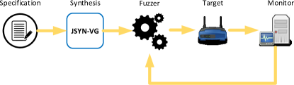
Figure 5. Fuzzer synthesis and testing diagram

The main intuition is that the SUT’s input description can be viewed as a substantial fragment of the fuzzer’s specification, which can then be used to synthesize a reactive random test case generator. Fig. 5 depicts our exact setup, where the designer already has a specification for the SUT and uses JSyn-vg with our Skolemization algorithm to automatically generate a corresponding fuzzer. The fuzzer is then attached to the SUT (Target), along with an accompanied monitoring service (Monitor) that tracks progress with respect to the SUT-related statistics (e.g., coverage). Following the definition of graybox fuzzing, a feedback loop exists where monitored information can be subsequently fed to the fuzzer, in order to dictate the generation of future test cases.

Table 1. Fuzzer performance comparison and synthesis times.

	AFL				AFLFast				Synthesized Fuzzer
	w/o corpus		w/ corpus		w/o corpus		w/ corpus
System Under Test	Coverage (%)	Crashed?	Coverage (%)	Crashed?	Coverage (%)	Crashed?	Coverage (%)	Crashed?	Coverage (%)	Crashed?	Synthesis times (s)
basic_messaging	83.76%	✘	82.48%	✘	82.48%	✘	82.48%	✘	81.21%	✔	16.067
Dive_Logger	92.18%	✘	92.41%	✘	92.18%	✘	92.18%	✘	93.79%	✔	99.852
Divelogger2	80.50%	✘	87.04%	✘	78.40%	✘	85.08%	✘	83.25%	✘	77.689
Email_System_2	78.71%	✘	92.90%	✘	91.61%	✘	92.90%	✘	84.84%	✔	36.624
Movie_Rental_Service	38.32%	✘	38.72%	✘	38.32%	✘	38.72%	✘	49.50%	✔	140.826
Palindrome	78.13%	✔	78.13%	✔	78.13%	✔	78.13%	✔	75.00%	✔	1.231
PTaaS	71.94%	✔	78.06%	✔	46.76%	✔	46.76%	✔	74.46%	✔	77.041
Quadtree_Conways	67.04%	✘	84.08%	✘	67.04%	✘	67.04%	✘	64.79%	✘	88.743
SCUBA_Dive_Logging	80.97%	✔	80.67%	✔	76.41%	✔	76.41%	✔	83.56%	✔	101.813
User_Manager	58.43%	✘	67.45%	✘	29.02%	✘	29.02%	✘	79.80%	✘	16.289

Using this setup, we proceeded with a thorough performance evaluation of our synthesized fuzzers, following guidelines that were recently proposed by Klees et al. (Klees et al., 2018):

SUT Selection. We considered ten applications from the DARPA Cyber Grand Challenge (CGC) , a benchmark collection that has been extensively used in the past to assess the performance of fuzzers due to the high degree of interactivity between the SUT and the user (Stephens et al., 2016; Rawat et al., 2017; Peng et al., 2018). The original collection was aimed towards the evaluation of automated reasoning and testing tools, and each application is intentionally documented in a way that is insufficient to derive a precise specification from the documents themselves. To simulate the context under which synthesis would make most sense as a tool, we closely inspected and ran each application in order to identify the types and sequences of inputs each application takes. The manual process of discovering and writing input specifications per application was non-trivial, as each application differs considerably from the rest, and was the main factor to the study being limited to a subset of ten applications.

Fuzzer specification. After inspecting each application to identify the kinds of inputs that it takes, we wrote a corresponding Assume-Guarantee contract for a fuzzer. Each fuzzer specification consists of properties that capture the valid ranges of values for each one of the SUT inputs. Moreover, the specification is stateful, making each fuzzer reactive to changes (or lack thereof) in coverage results from previously generated tests. We specified the behavior of the fuzzer in such a way that, for the majority of its runtime, valid inputs are fed into the SUT. As long as no progress is made in terms of coverage, the fuzzer attempts generating invalid tests with probability $p=0.2$.

Formalization. All of the aforementioned elements that comprise the fuzzer specification can be expressed using a set of safety properties over the SUT inputs, where each set precisely captures the conditions under which a (in)valid value is generated for the corresponding input. An example pair of such properties is the following:

• $prop_{1}\mathrel{\stackrel{{\scriptstyle\makebox[0.0pt]{\mbox{\tiny def}}}}{{=}}}p^{\prime}\geq 0\land p^{\prime}\leq 1$

• $prop_{2}\mathrel{\stackrel{{\scriptstyle\makebox[0.0pt]{\mbox{\tiny def}}}}{{=}}}(\lnot cvg\land(p\leq 0.1\lor p\geq 0.9))\Rightarrow in^{\prime}_{\text{sys}}\notin S_{\text{valid}}$

Variables $p$ and $in_{\text{sys}}$ are fuzzer outputs, with $in_{\text{sys}}$ also serving as a corresponding input for the SUT. The value of $p\in[0,1]$ is picked randomly for each test, and it determines whether the next (primed) system input $in^{\prime}_{\text{sys}}$ will be assigned to a valid value (i.e., a value in $S_{\text{valid}}$) or not. Variable $cvg$ is an input to the fuzzer and can be viewed as a flag which, when set, informs the fuzzer that the previous test resulted in progress in system coverage (e.g., line coverage improved). If such progress was not observed, then we allow the fuzzer to randomly consider invalid values in subsequent tests. More specifically, when $p\leq 0.1\lor p\geq 0.9$, the fuzzer will generate an invalid value, i.e., a value that does not satisfy the constraints that define $S_{\text{valid}}$. Following the notation that we described in previous sections, the synthesis problem for the properties above is to ensure that $\forall p,cvg,in_{\text{sys}}\exists p^{\prime},in^{\prime}_{\text{sys}}.(prop_{1}\land prop_{2})$ is valid.

Synthesis and Evaluation. Using the fuzzer contracts, we synthesized a fuzzer for each application and ran it against the SUT using the setup in Fig. 5. We set the timeout for each fuzzing campaign to nine hours, and monitored the SUT line coverage (gcov) as well as crashes. To compare performance, we also ran fuzzing campaigns using AFL (Zalewski, [n.d.]) and AFLFast (Böhme et al., 2017), using their default configurations. We selected these tools primarily due to AFL being one of the most prominent tools in the area, while AFLFast is a recent extension to AFL that has been shown to perform better with respect to vulnerability detection. Both tools were run both with and without an initial corpus in order to provide a more complete picture of their performance, whether the user provides additional information or not. To remain fair with respect to the evaluation, the corpora were created using tests that exercise application locations that are as deep as possible.

Table 1 shows the results of our experiments. Most of the applications contain unreachable code related to debugging methods, and as such 100% coverage is not attainable using gcov without further modifications to the source code. While we were able to achieve $\geq 75\%$ line coverage for the majority of the benchmarks, the application “Movie_Rental_Service” was the worst performing with only 49.5%. Despite that, the synthesized fuzzer outperformed both AFL and AFLFast on either configuration with a significant margin. In fact, our synthesized fuzzers outperformed both AFL and AFLFast on four applications and remained within 4% of the best performing tool for five others, with “Quadtree_Conways” being the only exception. More interestingly, seven of the synthesized fuzzers were able to crash the corresponding application at least once, whereas AFL/AFLFast were only able to crash three.

Considering the performance results along with the low synthesis time per fuzzer, we believe that synthesis of model-based fuzzers should be considered a viable tactic towards testing systems where a specification already exists. Arguably, a synthesized fuzzer is as easy to use as a general-purpose tool like AFL. Furthermore, the user does not have to provide additional information through a corpus, a procedure in testing that often times can be time consuming and cumbersome, as both valid and invalid input sequences have to be considered for a successful campaign.

7. Case Study 2: Robot Motion Planning

In our second study, we synthesized implementations for robots participating in two-player safety games against an adversary. The study is furthermore split into two parts.

7.1. Simulating avoidance games

We experimented on simulating an avoidance game in a bounded arena, where the synthesized solution was used against two different adversarial scenarios. Both the properties of the robot and the adversary were specified using their position in terms of $(x,y)$ coordinates. Formally, we described the game using the following properties:

• Initial state : The robot starts in $(x_{\text{init}},y_{\text{init}})$ (similarly for the adversary).

• Valid transitions : $x^{\prime}_{\text{robot}}\in[x_{\text{robot}}-\delta,x_{\text{robot}}+\delta]$, where $\delta$ is user-defined and captures the maximum distance between subsequent moves (similarly for $y$-coordinate and the adversarial transitions).

• In-bounds property : $x_{\text{robot}}\geq x_{\text{min}}\land x_{\text{robot}}\leq x_{\text{max}}$ (similarly for the $y$-coordinate).

• Avoidance property : $x_{\text{robot}}\neq x_{\text{adversary}}\lor y_{\text{robot}}\neq y_{\text{adversary}}$.

The first scenario in our presentation involves the adversary patrolling on a specific route, while in the second the adversary is always moving towards the robot. Trajectory videos for both scenarios are available online.

7.1.1. Real Coordinates.

Fig. 6 shows three possible trajectories that were generated after running the synthesized solution for 1000 turns against the patrolling adversary. Both robots move in the arena using rational coordinates in a 5x5 box. The initial location for the robot is the point $(0.5,0.5)$ and the adversary begins its route from $(0.8,0.8)$. While the adversary has a predetermined route, the robot is allowed to move towards any possible direction (vertically, horizontally and diagonally). Moreover, the robot can move at varying distances up to 0.1 units away from its current position, in both axes (i.e., $|x_{\text{robot}}-x^{\prime}_{\text{robot}}|\leq 0.1$, and similarly for the y axis). Fig. 6a indicates how the synthesized solution can respond in a random pattern, covering different parts of the bounded arena while preserving safety. Fig. 6b and 6c demonstrate the resulting trajectories when the user introduces bias in the values returned by the random number generators, using the same generated witness from AE-VAL. As a result, the robot was limited to moves that would retain its position within the central area of the arena (Fig. 6b) and close to the bottom left corner of the patrolling adversary’s route (Fig. 6c).

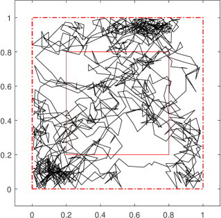
(a)

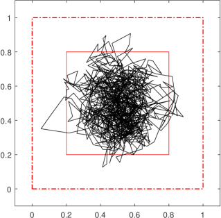
(b)

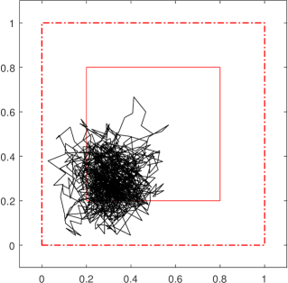
(c)

Figure 6. Random trajectories of a robot (irregular solid line) while avoiding a patrolling adversary (inner square).

7.1.2. Integer Coordinates.

For this experiment, we aimed to demonstrate the advantages that randomness can provide with respect to how well a robot covers a bounded arena, inspired by work in coverage path planning problems. Fig. 7 shows how two trajectories evolved over several turns (100, 250 and 1000 turns) for a similar motion planning problem using integer coordinates. To demonstrate which parts of the arena the robot explored we outline its trajectory with a bold black line, while the red line represents the trajectory of the adversary. In this game, the adversary is aggressively chasing after the robot in a random fashion. The robot’s objective remains the same, i.e., move within the bounded arena while avoiding the adversary. The robot’s initial location is the point $(0,0)$, while the adversary begins at $(6,6)$.

In fact, Fig. 7a, 7c, and 7e show moves performed by a random controller, while Fig. 7b, 7d,and  7f depict the behavior of the deterministic solution provided by the standard synthesis algorithm in JSyn-vg. It is apparent that the former visits 100% states in less than 250 turns, whereas the latter visits only 30% states in 1000 turns. This comparison showcases the advantages that a random solution can provide in terms of overall coverage as well as the diversity of behaviors that can be observed and exercised when an implementation can be generated that always considers the entire set of safe choices, instead of an instantiated strategy.

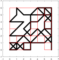
(a) 100 turns

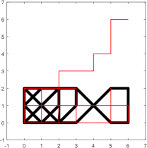
(b) 100 turns

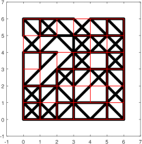
(c) 250 turns

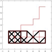
(d) 250 turns

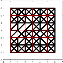
(e) 1000 turns

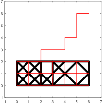
(f) 1000 turns

Figure 7. Trajectories and area coverage over time of random (left column) versus deterministic (right column) controller.

8. Evaluation – Synthesis time

Our case study in robot motion planning was inspired by results in this context from the most recent and related work on DT-Synth (Neider and Markgraf, 2019). This reactive synthesis framework incorporates learning techniques to generate winning sets for infinite-state safety games in the form of decision trees. DT-Synth has been shown to outperform previous proposed synthesis tools, both in infinite-state (ConSynth (Beyene et al., 2014a) and finite-state problems (RPNI-Synth and SAT-Synth (Neider and Topcu, 2016)). While the authors do not explicitly talk about randomness, the winning sets provided by DT-Synth are sufficient to generate implementations with diverse behavior. Despite this fact, the generated winning sets are subsets of the greatest fixpoint of safe states, which would lead to implementations that only exercise a fragment of the reachable state space. An example is the winning set that we mentioned for the motivating example in Section 3.

Note that DT-Synth works only for finite-branching game graphs, and the user must additionally specify a minimum value for the number of successors for each vertex in the graph. An incorrect value for this threshold can lead to unsound witnesses. With our JSyn-vg, such additional knowledge is not required from the user since it is only reliant on the original specification and is guaranteed to provide sound results, thanks to Theorem 4.5.

Table 2 presents the comparison of JSyn-vg and DT-Synth. As an addendum we included the synthesis times for the problems using the existing deterministic synthesis algorithm in JSyn-vg. As we mentioned in Sect. 5, the performance is identical when compared to synthesizing random witnesses.

For the purposes of this comparison, we used the infinite-state benchmarks presented in the original paper on DT-Synth (Neider and Markgraf, 2019), as well as the simulated avoidance games from Sect. 7.1, namely bounded_evasion and bounded_evasion_ints. The two tools have similar performance for half the benchmarks, with significant differences for the rest. For diagonal, the main distinction is that DT-Synth requires the definition of two additional expressions to guide the learning procedure, whereas JSyn-vg finds a solution without additional templates. On the other hand, DT-Synth’s ability to synthesize memoryless strategies allows for faster synthesis for solitarybox, where the robot is simply moving freely within an infinite arena while staying within a horizontal stripe of width equal to three. JSyn-vg is targeted to synthesis of stateful systems, and as such, a more elaborate strategy is generated.

In the case of repair-critical, DT-Synth appears to be more efficient in terms of handling disjunctive expressions in the specification, while for synth-synchronization DT-Synth seems to require more elaborate hypotheses in order to come up with a witness. The latter is further demonstrated in the results for the cinderella and bounded_evasion_ints games, where DT-Synth fails to synthesize a witness within the timeout of 15 minutes. In contrast, JSyn-vg computes a greatest fixpoint of safe states and synthesizes a solution in a few seconds. Finally, for the game bounded_evasion, DT-Synth does not currently support the theory of linear real arithmetic.

Table 2. Synthesis time of DT-Synth and JSyn-vg (seconds).

Benchmark	JSyn-vg	JSyn-vg (random)	DT-Synth
box	0.603	0.606	0.258
diagonal	1.109	1.011	6.027
evasion	0.705	0.605	0.660
follow	3.34	3.029	1.034
limitedbox	3.229	3.332	3.350
solitarybox	1.902	1.816	0.284
square	5.823	5.605	6.44
program-repair	3.122	3.638	2.452
repair-critical	83.891	88.073	30.593
synth-synchronization	23.013	23.2	89.804
cinderella ($c=2$)	20.061	20.167	$>900$
cinderella ($c=3$)	12.02	11.294	$>900$
bounded_evasion	49.528	49.662	unsupported
bounded_evasion_ints	31.614	32.611	$>900$

9. Related Work

The idea of synthesizing reactive designs with random behavior is relevant to synthesis for permissive games. This area has been explored in the past for finite-state problems (Bouyer et al., 2009; Könighofer et al., 2017). More recently, Fremont and Seshia described a formal extension to the theory of Control Improvisation to support reactive synthesis (Fremont and Seshia, 2018). Their probabilistic approach is limited to finite-state problems and practically useful only for the subset of safety games. The end result is a maximally-randomized finite word generator, called an improviser, where each word satisfies the predetermined probability threshold constraints. In comparison, our approach synthesizes designs for infinite-state problems that simulate randomness. Furthermore, we do not provide guarantees regarding the randomness of the responses from the synthesized witness. Instead, we focus on synthesizing witnesses that consider regions of values as candidates to variable assignments, a problem reducible to SMT. In our case, the end product is an implementation that can be further refined by the engineer with a custom probability distribution to retrieve random values. This provides invaluable freedom as the user can then choose whether to express bias through the requirements or through the random number generators themselves.

The original work on JSyn-vg targeted the area of infinite-state problems. In this context, Beyenne et al. first proposed a template-based approach called ConSynth, where the specification is accompanied by a template regarding the shape of the solution to guide the synthesizer towards a solution (Beyene et al., 2014b). In contrast, JSyn-vg is a completely automated approach exempting the user from necessity to further reason about the shape of the computed solution and allowing to focus on expressing the problem in the form of input-output contracts. Permissive solutions for infinite-state games have primarily been proposed in the context supervisor synthesis (Claessen et al., 2017; Shoaei et al., 2014), where a controller is synthesized considering a formal representation of the behavior (inputs) provided by the participating plant. Compared to this work, our proposed solution explores the applicability of synthesized controllers with random behavior, while the overall synthesis task is inherently harder due to not requiring an exact implementation of the controller’s environment.

Neider and Markgraf recently proposed DT-Synth (Neider and Markgraf, 2019), a learning-based approach to synthesizing winning sets for infinite state games in the form of decision trees, as an extension to previous work by Neider and Topcu for finite-state problems (Neider and Topcu, 2016). DT-Synth requires additional knowledge regarding the number of successor states, where lack thereof can lead to unsound results. Similarly to ConSynth, for more complex problems, the game specification is supported by additional syntactic expressions that help the learner converge faster to a solution. In contrast, our Skolem extraction algorithm is guaranteed to provide sound witnesses and does not depend on additional user-provided input.

10. Conclusion

We have presented a novel Skolemization procedure for the AE-VAL solver enabling the synthesis of infinite-state reactive implementations with random behavior. The proposed solution is an extension to the synthesis algorithm JSyn-vg that computes a greatest fixpoint of safe states. The product is a witness where values inside safe regions are being considered as equally safe candidate assignments. Our solution provides the engineer with flexibility when it comes to introducing additional bias through the specification or the implemented random number generators.

To the best of our knowledge, this is the first work that is capable of synthesizing random infinite-state systems. We showed how the extended synthesis framework can be effectively used to synthesize promising solutions in the context of robot motion planning, as well as a novel application in fuzz testing. In the future, we wish to continue exploring the area of reactive fuzzer synthesis, particularly in the context of identifying a formal specification standard. To expand its applicability in robot motion planning, we wish to explore ways to support liveness specifications, as well as soft requirements. The outstanding result of this work is a Skolem extraction procedure general enough to be applicable to other, unexplored, aspects of the synthesis problem.

- (1)
- pea ([n.d.]) [n.d.]. Peach fuzzer. https://www.peach.tech/.
- Abate et al. (2017) Alessandro Abate, Iury Bessa, Dario Cattaruzza, Lucas Cordeiro, Cristina David, Pascal Kesseli, Daniel Kroening, and Elizabeth Polgreen. 2017. Automated formal synthesis of digital controllers for state-space physical plants. In International Conference on Computer Aided Verification. Springer, 462–482.
- Alur et al. (2013) Rajeev Alur, Rastislav Bodik, Garvit Juniwal, Milo MK Martin, Mukund Raghothaman, Sanjit A Seshia, Rishabh Singh, Armando Solar-Lezama, Emina Torlak, and Abhishek Udupa. 2013. Syntax-guided synthesis. In 2013 Formal Methods in Computer-Aided Design. IEEE, 1–8.
- Aschermann et al. (2019) Cornelius Aschermann, Tommaso Frassetto, Thorsten Holz, Patrick Jauernig, Ahmad-Reza Sadeghi, and Daniel Teuchert. 2019. NAUTILUS: Fishing for Deep Bugs with Grammars.. In NDSS.
- Barrett et al. (2010) Clark Barrett, Aaron Stump, Cesare Tinelli, et al. 2010. The smt-lib standard: Version 2.0. In Proceedings of the 8th International Workshop on Satisfiability Modulo Theories (Edinburgh, England), Vol. 13. 14.
- Beyene et al. (2014a) Tewodros Beyene, Swarat Chaudhuri, Corneliu Popeea, and Andrey Rybalchenko. 2014a. A constraint-based approach to solving games on infinite graphs. In POPL. ACM, 221–233.
- Beyene et al. (2014b) Tewodros A. Beyene, Swarat Chaudhuri, Corneliu Popeea, and Andrey Rybalchenko. 2014b. A constraint-based approach to solving games on infinite graphs. In POPL. ACM, 221–234.
- Bjørner and Janota (2015) Nikolaj Bjørner and Mikolás Janota. 2015. Playing with Quantified Satisfaction. In LPAR (short papers) (EPiC Series in Computing), Vol. 35. EasyChair, 15–27.
- Böhme et al. (2017) Marcel Böhme, Van-Thuan Pham, and Abhik Roychoudhury. 2017. Coverage-based greybox fuzzing as markov chain. IEEE Transactions on Software Engineering 45, 5 (2017), 489–506.
- Bouyer et al. (2009) Patricia Bouyer, Marie Duflot, Nicolas Markey, and Gabriel Renault. 2009. Measuring permissivity in finite games. In International Conference on Concurrency Theory. Springer, 196–210.
- Chakraborty et al. (2018) Supratik Chakraborty, Dror Fried, Lucas M Tabajara, and Moshe Y Vardi. 2018. Functional synthesis via input-output separation. In 2018 Formal Methods in Computer Aided Design (FMCAD). IEEE, 1–9.
- Champion et al. (2016) Adrien Champion, Alain Mebsout, Christoph Sticksel, and Cesare Tinelli. 2016. The Kind 2 model checker. In International Conference on Computer Aided Verification. Springer, 510–517.
- Claessen et al. (2017) Koen Claessen, Jonatan Kilhamn, Laura Kovács, and Bengt Lennartson. 2017. A Supervisory Control Algorithm Based on Property-Directed Reachability. In Haifa Verification Conference. Springer, 115–130.
- Fedyukovich and Gupta (2019) Grigory Fedyukovich and Aarti Gupta. 2019. Functional Synthesis with Examples. In CP (LNCS), Vol. 11802. Springer, 547–564.
- Fedyukovich et al. (2019) Grigory Fedyukovich, Arie Gurfinkel, and Aarti Gupta. 2019. Lazy but Effective Functional Synthesis. In VMCAI (LNCS), Vol. 11388. Springer, 92–113.
- Fedyukovich et al. (2015) Grigory Fedyukovich, Arie Gurfinkel, and Natasha Sharygina. 2015. Automated Discovery of Simulation Between Programs. In LPAR (LNCS), Vol. 9450. Springer, 606–621.
- Finkbeiner (2016) Bernd Finkbeiner. 2016. Synthesis of Reactive Systems. Dependable Software Systems Engineering 45 (2016), 72–98.
- Fraze ([n.d.]) Dustin Fraze. [n.d.]. The DARPA Cyber Grand Challenge. https://www.darpa.mil/program/cyber-grand-challenge.
- Fremont et al. (2017) Daniel J Fremont, Alexandre Donzé, and Sanjit A Seshia. 2017. Control improvisation. arXiv preprint arXiv:1704.06319 (2017).
- Fremont and Seshia (2018) Daniel J. Fremont and Sanjit A. Seshia. 2018. Reactive Control Improvisation. In Computer Aided Verification, Hana Chockler and Georg Weissenbacher (Eds.). Springer International Publishing, Cham, 307–326.
- Gacek et al. (2018) Andrew Gacek, John Backes, Mike Whalen, Lucas Wagner, and Elaheh Ghassabani. 2018. The JKind Model Checker. In International Conference on Computer Aided Verification. Springer, 20–27.
- Gacek et al. (2015) Andrew Gacek, Andreas Katis, Michael W Whalen, John Backes, and Darren Cofer. 2015. Towards Realizability Checking of Contracts Using Theories. In NFM (LNCS), Vol. 9058. Springer, 173–187.
- Galceran and Carreras (2013) Enric Galceran and Marc Carreras. 2013. A survey on coverage path planning for robotics. Robotics and Autonomous systems 61, 12 (2013), 1258–1276.
- Gulwani (2010) Sumit Gulwani. 2010. Dimensions in program synthesis. In PPDP. ACM, 13–24.
- Holler et al. (2012) Christian Holler, Kim Herzig, and Andreas Zeller. 2012. Fuzzing with code fragments. In Presented as part of the 21st USENIX Security Symposium (USENIX Security 12). 445–458.
- Howar and Steffen (2018) Falk Howar and Bernhard Steffen. 2018. Active automata learning in practice. In Machine Learning for Dynamic Software Analysis: Potentials and Limits. Springer, 123–148.
- Jahier et al. ([n.d.]) Erwan Jahier, Pascal Raymond, and Nicolas Halbwachs. [n.d.]. The Lustre V6 Reference Manual. http://www-verimag.imag.fr/Lustre-V6.html.
- Katis et al. (2018) Andreas Katis, Grigory Fedyukovich, Huajun Guo, Andrew Gacek, John Backes, Arie Gurfinkel, and Michael W Whalen. 2018. Validity-guided synthesis of reactive systems from assume-guarantee contracts. In International Conference on Tools and Algorithms for the Construction and Analysis of Systems. Springer, 176–193.
- Katis et al. (2015) Andreas Katis, Andrew Gacek, and Michael W Whalen. 2015. Machine-Checked Proofs For Realizability Checking Algorithms. In VSTTE. Springer, 110–123.
- Katis et al. (2016) Andreas Katis, Andrew Gacek, and Michael W Whalen. 2016. Towards synthesis from assume-guarantee contracts involving infinite theories: a preliminary report. In FormaliSE. IEEE, 36–41.
- Klees et al. (2018) George Klees, Andrew Ruef, Benji Cooper, Shiyi Wei, and Michael Hicks. 2018. Evaluating fuzz testing. In Proceedings of the 2018 ACM SIGSAC Conference on Computer and Communications Security. 2123–2138.
- Könighofer et al. (2017) Bettina Könighofer, Mohammed Alshiekh, Roderick Bloem, Laura Humphrey, Robert Könighofer, Ufuk Topcu, and Chao Wang. 2017. Shield synthesis. Formal Methods in System Design 51, 2 (2017), 332–361.
- Lee (2015) Newton Lee. 2015. DARPA’s Cyber Grand Challenge (2014–2016). In Counterterrorism and Cybersecurity. Springer, 429–456.
- Manès et al. (2019) Valentin Jean Marie Manès, HyungSeok Han, Choongwoo Han, Sang Kil Cha, Manuel Egele, Edward J Schwartz, and Maverick Woo. 2019. The art, science, and engineering of fuzzing: A survey. IEEE Transactions on Software Engineering (2019).
- Neider and Markgraf (2019) Daniel Neider and Oliver Markgraf. 2019. Learning-based synthesis of safety controllers. In 2019 Formal Methods in Computer Aided Design (FMCAD). IEEE, 120–128.
- Neider and Topcu (2016) Daniel Neider and Ufuk Topcu. 2016. An automaton learning approach to solving safety games over infinite graphs. In International Conference on Tools and Algorithms for the Construction and Analysis of Systems. Springer, 204–221.
- Nguyen et al. (2017) ThanhVu Nguyen, Westley Weimer, Deepak Kapur, and Stephanie Forrest. 2017. Connecting program synthesis and reachability: Automatic program repair using test-input generation. In International Conference on Tools and Algorithms for the Construction and Analysis of Systems. Springer, 301–318.
- Peng et al. (2018) Hui Peng, Yan Shoshitaishvili, and Mathias Payer. 2018. T-Fuzz: fuzzing by program transformation. In 2018 IEEE Symposium on Security and Privacy (SP). IEEE, 697–710.
- Pham et al. (2016) Van-Thuan Pham, Marcel Böhme, and Abhik Roychoudhury. 2016. Model-based whitebox fuzzing for program binaries. In Proceedings of the 31st IEEE/ACM International Conference on Automated Software Engineering. 543–553.
- Rash ([n.d.]) Michael Rash. [n.d.]. afl-cov - AFL Fuzzing Code Coverage. https://github.com/mrash/afl-cov.
- Rawat et al. (2017) Sanjay Rawat, Vivek Jain, Ashish Kumar, Lucian Cojocar, Cristiano Giuffrida, and Herbert Bos. 2017. VUzzer: Application-aware Evolutionary Fuzzing.. In NDSS, Vol. 17. 1–14.
- Ryzhyk et al. (2009) Leonid Ryzhyk, Peter Chubb, Ihor Kuz, Etienne Le Sueur, and Gernot Heiser. 2009. Automatic device driver synthesis with Termite. In Proceedings of the ACM SIGOPS 22nd symposium on Operating systems principles. ACM, 73–86.
- Shoaei et al. (2014) Mohammad Reza Shoaei, Laura Kovács, and Bengt Lennartson. 2014. Supervisory control of discrete-event systems via IC3. In Haifa Verification Conference. Springer, 252–266.
- Stephens et al. (2016) Nick Stephens, John Grosen, Christopher Salls, Andrew Dutcher, Ruoyu Wang, Jacopo Corbetta, Yan Shoshitaishvili, Christopher Kruegel, and Giovanni Vigna. 2016. Driller: Augmenting Fuzzing Through Selective Symbolic Execution.. In NDSS, Vol. 16. 1–16.
- Utting et al. (2012) Mark Utting, Alexander Pretschner, and Bruno Legeard. 2012. A taxonomy of model-based testing approaches. Software testing, verification and reliability 22, 5 (2012), 297–312.
- Veggalam et al. (2016) Spandan Veggalam, Sanjay Rawat, Istvan Haller, and Herbert Bos. 2016. Ifuzzer: An evolutionary interpreter fuzzer using genetic programming. In European Symposium on Research in Computer Security. Springer, 581–601.
- Zalewski ([n.d.]) Michal Zalewski. [n.d.]. American Fuzzy Lop. https://lcamtuf.coredump.cx/afl/.