Gribov-Zwanziger confinement, high energy evolution and large impact parameter behaviour of the scattering amplitude

Abstract

In this paper we derive the high energy evolution equation in the Gribov-Zwanziger approach, for the confinement of quarks and gluons. We demonstrate that the new equation generates an exponential decrease of the scattering amplitude at large impact parameter, and resolves the main difficulties of CGC (Colour Glass Condensate) high energy effective theory. Such behaviour occurs, if the gluon propagator in Gribov-Zwanziger approach, does not vanish at small momenta. Solving the non-linear equation for deep inelastic scattering, we show that the suggested equation leads to a Froissart disc with radius ($R_{F}$), which increases as $R_{F}\,\propto Y=\ln(1/x)$, and with a finite width for the distribution over $|b-R_{F}|$.

I Introduction

It is well known that the Balitsky-Kovchegov equationBK :

$$\frac{\partial}{\partial Y}N\left(\boldsymbol{r},\boldsymbol{b},Y\right) = \bar{\alpha}_{S}\!\!\int\frac{d^{2}\boldsymbol{r}^{\prime}}{2\,\pi}\,K\left(\boldsymbol{r}^{\prime},\boldsymbol{r}-\boldsymbol{r}^{\prime};\boldsymbol{r}\right)\Bigg{\{}N\left(\boldsymbol{r}^{\prime},\boldsymbol{b}-\frac{1}{2}\left(\boldsymbol{r}-\boldsymbol{r}^{\prime}\right),Y\right)+N\left(\boldsymbol{r}-\boldsymbol{r}^{\prime},\boldsymbol{b}-\frac{1}{2}\boldsymbol{r}^{\prime},Y\right)\,\,-\,\,N\left(\boldsymbol{r},\boldsymbol{b},Y\right)$$ (1)

$$~{}~{}~{}~{}~{}~{}~{}-N\left(\boldsymbol{r}-\boldsymbol{r}^{\prime},\boldsymbol{b}-\frac{1}{2}\boldsymbol{r}^{\prime},Y\right)\,N\left(\boldsymbol{r}^{\prime},\boldsymbol{b}-\frac{1}{2}\left(\boldsymbol{r}-\boldsymbol{r}^{\prime}\right),Y\right)\Bigg{\}}$$

generates a scattering amplitude which decreases as a power of $b$ at large impact parameter (see Ref.KOLEB for review).

In Eq. (1) the kernel $K\left(\boldsymbol{r}^{\prime},\boldsymbol{r}-\boldsymbol{r}^{\prime};\boldsymbol{r}\right)$ describes the decay of the dipole of size $r$, into two dipoles with sizes $r^{\prime}$ and $|\boldsymbol{r}\,-\,\boldsymbol{r}^{\prime}|$, respectively. It has the form:

$$K\left(\boldsymbol{r}^{\prime},\boldsymbol{r}-\boldsymbol{r}^{\prime};\boldsymbol{r}\right)\,\,=\,\,\frac{r^{2}}{r^{\prime 2}\,\left(\boldsymbol{r}-\boldsymbol{r}^{\prime}\right)^{2}}$$ (2)

Indeed, at large $b$ we can neglect the non-linear term in Eq. (1), and the linear BFKL equationFKL ; BFKL determines the large $b$ behaviour. It is known that the eigenfunction of this equation (the scattering amplitude of two dipoles with sizes $r$ and $R$) has the following form LIP

$$\phi_{\gamma}\left(\boldsymbol{r},\boldsymbol{R},\boldsymbol{b}\right)\,\,\,=\,\,\,\left(\frac{r^{2}\,R^{2}}{\left(\boldsymbol{b}+\frac{1}{2}(\boldsymbol{r}-\boldsymbol{R})\right)^{2}\,\left(\boldsymbol{b}-\frac{1}{2}(\boldsymbol{r}-\boldsymbol{R})\right)^{2}}\right)^{\gamma}\,\,\xrightarrow{b\,\gg\,r,R}\,\,\left(\frac{r^{2}\,R^{2}}{b^{4}}\right)^{\gamma}\,\,\equiv\,\,e^{\gamma\,\xi}~{}~{}\mbox{with}~{}~{}\xi\,=\,\ln\left(\frac{r^{2}\,R^{2}}{b^{4}}\right)$$ (3)

Eq. (3) shows the power-like decrease at large $b$, which leads to the violation of the Froissart theoremFROI generating a cross section, which at high energies increases as a power of energy KW ; FIIM . The solution of this problem requires introducing a new dimensional scale. A variety of ideas to overcome this problem have been suggested in Refs. LERYB1 ; LERYB2 ; LETAN ; QCD2 ; KHLEP ; KKL ; FIIM ; GBS1 ; BLT ; GKLMN ; HAMU ; MUMU ; BEST1 ; BEST2 ; KOLE ; LETA ; LLS ; LEPION ; KHLE ; KAN ; GOLEB . In this paper we intend to use the Gribov-Zwanziger approachGRI0 ; GRI1 ; GRI2 ; GRI3 ; GRI4 ; GRREV ; DOKH for the confinement of quarks and gluons. In particular, we will use the Gribov gluon propagator in a form which describes the recent lattice QCD estimates DOS .

The plan of this paper is as follows. In the next section we illustrate the problem of the large impact parameter behaviour of the BK equation as an example of the first iterations of this equation. In section III we discuss the model: non-abelian gauge theories with Higgs mechanism of mass generation, which has been suggested in Ref.LLS for high energy scattering. In spite of the fact that this model does not have the confinement of quarks and gluons, we found it instructive to reproduce the large impact parameter behaviour of the scattering amplitude in this model. It should be stressed that this model not only leads to the exponential decrease of the scattering amplitude at large $b$, but has the same spectrum of energies as the massless BFKL equation in QCD. Section IV is the key chapter in the paper. It contains a discussion of the modification of the BFKL evolution equation for the Gribov-Zwanziger approach, to the confinement problem. We show that this mechanism of confinement introduces a new dimensional parameter, and it leads to the exponential decrease of the scattering amplitude at large $b$, only if the gluon propagator does not vanish at zero momentum. In other words, we need to introduce two dimensional parameters to provide the correct large $b$ behaviour in the framework of the Gribov-Zwanziger approach to confinement. In section V we discuss the non-linear equation with a generalized kernel, and show that this equation generates the Froissart- type behaviour of the scattering amplitude with a radius which increase as $Y=\ln(1/x)$. Finally, in Section VI we discuss our results and future prospects.

II Iterations of BK equation

We start illustrating the problem of large $b$ behaviour with the first iteration of Eq. (1). At large $b$, we can neglect the non-linear term and concentrate our efforts on solution of linear BFKL FKL ; BFKL equation . The general initial condition $N^{(0)}$ generates the Green’s function in the impact parameter representation, and has the following form:

$$N^{(0)}\,\,=\,\,r^{2}\,\delta^{(2)}\left(\boldsymbol{b}\right)$$ (4)

Eq. (4) gives the dimensionless function which plays the role of the Green’s function in $b$-space.

Plugging this initial condition in Eq. (1), one can see that we obtain the first iteration in the form:

$$N^{(1)}\left(\boldsymbol{r},\boldsymbol{b},Y\right)\,\,=\,\,\bar{\alpha}_{S}\,Y\,\Bigg{\{}\frac{1}{\pi}\,\frac{r^{2}}{\left(2\,\boldsymbol{b}\right)^{2}}\,\,\,-\,\ln r^{2}\,\,N^{(0)}\left(\boldsymbol{r},\boldsymbol{b}\right)\Bigg{\}}$$ (5)

Therefore, one can see that the initial conditions which have a sharp decrease in $b$, generate the power-like dependence of the solution to the BFKL equation. The next iteration leads to

$$N^{(2)}\left(\boldsymbol{r},\boldsymbol{b},Y\right)\,\,=\,\,\frac{1}{2}\left(\bar{\alpha}_{S}\,Y\right)^{2}\int d^{2}r^{\prime}2\,\frac{r^{2}}{\left(\boldsymbol{r}\,-\,\boldsymbol{r}^{\prime}\right)^{2}}\frac{1}{\left(2\,\boldsymbol{b}\right)^{2}}\,\,\xrightarrow{b\gg r^{\prime}\gg r}\,\,\frac{1}{2}\left(\bar{\alpha}_{S}\,Y\right)^{2}\,\,\int^{b^{2}}_{r^{2}}\frac{dr^{\prime 2}}{r^{\prime 2}}\frac{r^{2}}{b^{2}}$$ (6)

Therefore, the BFKL equation generates the power-like decrease of the scattering amplitude in the first iteration, while in the following iterations the typical $r^{\prime}$ turns out to be much smaller than $b$.

It is instructive to recall that the power-like decrease, which comes from the integration over $r^{\prime}$ in Eq. (5), corresponds to the gluon reggeization term in the momentum representation. Indeed, in the momentum representation the BFKL equation takes the formFKL ; BFKL :

$$\frac{\partial N\left(Y;q,Q_{T}\right)}{\partial Y}\,\, = \,\,\bar{\alpha}_{S}\Bigg{(}\int\frac{d^{2}q^{\prime}}{2\pi}K_{\rm em}\left(\boldsymbol{q}-\boldsymbol{q}^{\prime},\boldsymbol{Q}_{T}\right)N\left(Y;q^{\prime},Q_{T}\right)\,\,-\,\,K_{\rm reg}\left(\boldsymbol{q}-\boldsymbol{q}^{\prime},\boldsymbol{Q}_{T}\right)N\left(Y;q,Q_{T}\right)\Bigg{)}$$

$$= \bar{\alpha}_{S}\,\int\frac{d^{2}q^{\prime}}{2\pi}K_{\rm em}\left(\boldsymbol{q}-\boldsymbol{q}^{\prime},\boldsymbol{Q}_{T}\right)N\left(Y;q^{\prime},Q_{T}\right)\,\,-\,\,\omega_{G}\left(q^{\prime}\right)\,\,-\,\,\omega_{G}\left(\boldsymbol{Q}_{T}\,-\,\boldsymbol{q^{\prime}}\right)$$

$$= \,\,\bar{\alpha}_{S}\int\frac{d^{2}q^{\prime}}{2\pi}K\left(\boldsymbol{q}-\boldsymbol{q}^{\prime},\boldsymbol{Q}_{T}\right)N\left(Y;q^{\prime},Q_{T}\right)$$ (7)

where $\bar{\alpha}_{S}=\left(N_{c}/\pi\right)\alpha_{S}$. The kernel $K_{\rm em}$ describes the emission of a gluon, while kernel $K_{\rm reg}$ is responsible for the reggeization of gluons in t-channel. They have the forms:

$$K_{\rm em}\left(\boldsymbol{q}-\boldsymbol{q}^{\prime},\boldsymbol{Q}_{T}\right)\,\, = \,\,\frac{1}{2}\frac{1}{\left(\boldsymbol{q}-\boldsymbol{q}^{\prime}\right)^{2}}\Bigg{\{}-\frac{Q^{2}_{T}\left(\boldsymbol{q}-\boldsymbol{q}^{\prime}\right)^{2}}{\left(\boldsymbol{Q}_{T}-\boldsymbol{q}^{\prime}\right)^{2}\,q^{\prime 2}}\,+1\,+\frac{\left(\boldsymbol{Q}_{T}-\boldsymbol{q}\right)^{2}\,q^{\prime 2}}{\left(\boldsymbol{Q}_{T}-\boldsymbol{q}^{\prime}\right)^{2}\,q^{2}}\Bigg{\}}\xrightarrow{Q_{T}=0}\frac{1}{\left(\boldsymbol{q}-\boldsymbol{q}^{\prime}\right)^{2}}$$ (8)

$$K_{\rm reg}\left(\boldsymbol{q}-\boldsymbol{q}^{\prime},\boldsymbol{Q}_{T}\right)\,\, = \frac{1}{2}\frac{1}{\left(\boldsymbol{q}-\boldsymbol{q}^{\prime}\right)^{2}}\Bigg{\{}\frac{q^{2}}{\left(\boldsymbol{q}-\boldsymbol{q}^{\prime}\right)^{2}\,+\,q^{\prime 2}}\,\,+\,\,\frac{\left(\boldsymbol{Q}_{T}\,-\,\boldsymbol{q}\right)^{2}}{\left(\boldsymbol{q}-\boldsymbol{q}^{\prime}\right)^{2}\,+\,\left(\boldsymbol{Q}_{T}-\boldsymbol{q}^{\prime}\right)^{2}}\Bigg{\}}\xrightarrow{Q_{T}=0}\frac{1}{\left(\boldsymbol{q}-\boldsymbol{q}^{\prime}\right)^{2}}\frac{q^{2}}{\left(\boldsymbol{q}-\boldsymbol{q}^{\prime}\right)^{2}\,+\,q^{\prime 2}}$$

$K\left(\boldsymbol{q}-\boldsymbol{q}^{\prime},\boldsymbol{Q}_{T}\right)$ is equal to

$$K\left(\boldsymbol{q}-\boldsymbol{q}^{\prime},\boldsymbol{Q}_{T}\right)N\left(Y;q^{\prime},Q_{T}\right)\,\,=\,\,K_{\rm em}\left(\boldsymbol{q}-\boldsymbol{q}^{\prime},\boldsymbol{Q}_{T}\right)N\left(Y;q^{\prime},Q_{T}\right)\,\,-\,\,K_{\rm reg}\left(\boldsymbol{q}-\boldsymbol{q}^{\prime},\boldsymbol{Q}_{T}\right)N\left(Y;q,Q_{T}\right)$$ (9)

The gluon trajectory $\omega_{G}\left(q\right)$ is equal to

$$\omega_{G}\left(q\right)\,\,=\,\,\bar{\alpha}_{S}\,\int\frac{d^{2}\,q^{\prime}}{4\,\pi}\,\frac{q^{2}}{q^{\prime 2}\,\left(\boldsymbol{q}\,-\,\boldsymbol{q}^{\prime}\right)^{2}}$$ (10)

The reggeization term of Eq. (II) leads to the power-like behaviour at large impact parameter. Therefore, we need to understand, what type of non-perturbative corrections could change this reggeization kernel to provide the exponential decrease, of the scattering amplitude at large impact parameters.

III The model: nonabelian gauge theories with the Higgs mechanism for mass generation.

III.1 BFKL equation

In this section we wish to answer the question: what is the large impact parameter behaviour in the non-abelian Yang-Mills theories with a Higgs particle. In these theories, we introduce the non-perturbative scale as the mass of Higgs, and we would like to see how this dimensional scale manifests itself in the large $b$ behaviour of the scattering amplitude. It was shown by Fadin, Lipatov and Kuraev FKL , that the high energy amplitude satisfies the BFKL equation (see Fig. 1) which has been written for colour $SU(N_{c})$, ($N_{c}$ is the number of colours) with the Higgs mechanism of mass generation, in Ref.LLS .

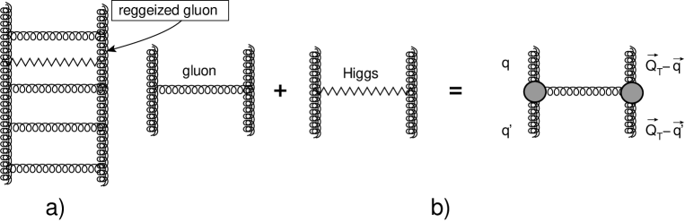
Figure 1: The massive BFKL equation (Fig. 1-a) and its kernel (Fig. 1-b)

It has the form of Eq. (II), with the kernels that have the following forms:

$$K_{\rm em}\left(\boldsymbol{q}-\boldsymbol{q}^{\prime},\boldsymbol{Q}_{T}\right)\,\, = \frac{1}{\left(\boldsymbol{q}\,-\,\boldsymbol{q}^{\prime}\right)^{2}+m^{2}}\Bigg{(}\frac{q^{2}_{1}+m^{2}}{q^{\prime 2}+m^{2}}\,+\,\frac{\left(\boldsymbol{Q}_{T}\,-\,\boldsymbol{q}\right)^{2}+m^{2}}{\left(\boldsymbol{Q}_{T}\,-\,\boldsymbol{q}^{\prime}\right)^{2}+m^{2}}\Bigg{)}\,\,-\,\,\frac{q^{2}+\frac{N^{2}_{c}+1}{N^{2}_{c}}m^{2}}{(q^{\prime 2}+m^{2})(\left(\boldsymbol{Q}_{T}\,-\,\boldsymbol{q}\right)^{2}+m^{2})}\;$$ (11a)

$$\omega_{G}\left(q\right)\,\, = \,\,\int\frac{d^{2}q^{\prime}}{4\,\pi}\frac{\left(q^{2}+m^{2}\right)}{\left(q^{\prime 2}+m^{2}\right)\left(\left(\boldsymbol{q}-\boldsymbol{q}^{\prime}\right)^{2}+m^{2}\right)}=\,\,\frac{1}{2}\frac{q^{2}+m^{2}}{|q|\sqrt{q^{2}+4m^{2}}}\ln\frac{\sqrt{q^{2}+4m^{2}}+|q|}{\sqrt{q^{2}+4m^{2}}-|q|}$$ (11b)

As one can see from Eq. (11b), $\omega_{G}\left(q\right)$ has singularities at $q^{2}\,=\,-4\,m^{2}$, which will generate the exponential decrease of the scattering amplitude at large $b$. As we have mentioned, the reggeization terms in coordinate representation generate the first term in Eq. (1). Using formulae 8.411(1), 8.411(7) and 6.532(4) of Ref. RY ) we obtain

$$\int\frac{d^{2}q^{\prime}}{2\pi}\frac{e^{i\boldsymbol{r}\cdot\boldsymbol{q}^{\prime}}}{q^{\prime 2}+m^{2}}\,=\,\int^{+\infty}_{-\infty}\frac{q^{\prime}dq^{\prime}\,J_{0}\left(rq^{\prime}\right)}{q^{\prime 2}+m^{2}}\,\,=\,\,K_{0}\left(rm\right)$$ (12)

where $J_{0}\left(z\right)$ and $K_{0}\left(z\right)$ are the Bessel functions of the first and second kinds, respectively (see Ref. RY ). Bearing Eq. (12) in mind, one can see that coordinate image of the gluon trajectory can be written as follows:

$$\omega_{G}\left(r\right)\,\,\, = \,\,\frac{1}{2}\,\left(-\nabla^{2}\,\,+\,\,m^{2}\right)\,K^{2}_{0}\left(r\,m\right)\,\,=\,\,-\,\,\frac{1}{2}\,\,m^{2}\Big{(}2K^{2}_{1}\left(m\,r\right)\,+\,K^{2}_{0}\left(m\,r\right)\Big{)}$$ (13a)

$$\xrightarrow{m\,\to\,0} -\frac{1}{r^{2}};$$ (13b)

$$\xrightarrow{r\,\to\,0} -\frac{1}{r^{2}}\,\,+\,\,\frac{1}{2}\,m^{2}\Big{(}2-\left(C\,+\,\ln\left(\frac{m\,r}{2}\right)\right)^{2}\Big{)};$$ (13c)

$$\xrightarrow{r\,\to\,\infty} \,e^{-2\,m\,r}\Big{(}-\frac{3\,m\,\pi}{4\,r}\,\,-\,\,\frac{5\,\pi}{16\,r^{2}}\Big{)};$$ (13d)

where $K_{1}\left(z\right)$ is the Bessel functions of the second kind and $C$ is the Euler constant.

The emission term of BFKL equation in coordinate representation(the first two terms in Eq. (1)) have the following form:

$$\frac{\partial}{\partial Y}N\left(\boldsymbol{r},\boldsymbol{b},Y\right)\,\,=\,\,-\bar{\alpha}_{S}\!\!\int\frac{d^{2}\boldsymbol{r}^{\prime}}{2\,\pi}\,\omega_{G}\left(\boldsymbol{r}-\boldsymbol{r}^{\prime}\right)N\left(\boldsymbol{r}^{\prime},\boldsymbol{b}-\frac{1}{2}\left(\boldsymbol{r}-\boldsymbol{r}^{\prime}\right),Y\right)$$ (14)

We need to add the contribution of $K_{\rm em}\left(\boldsymbol{q}-\boldsymbol{q}^{\prime},\boldsymbol{Q}_{T}\right)$ in the coordinate representation, which leads to the term proportional to $N\left(\boldsymbol{r},\boldsymbol{b},Y\right)$. Finally, the BFKL equation in the coordinate representation has the form:

$$\frac{\partial}{\partial Y}N\left(\boldsymbol{r},\boldsymbol{b},Y\right)\,\,=\,\,-\bar{\alpha}_{S}\!\!\int\frac{d^{2}\boldsymbol{r}^{\prime}}{2\,\pi}\,\omega_{G}\left(\boldsymbol{r}-\boldsymbol{r}^{\prime}\right)\Bigg{\{}N\left(\boldsymbol{r}^{\prime},\boldsymbol{b}-\frac{1}{2}\left(\boldsymbol{r}-\boldsymbol{r}^{\prime}\right),Y\right)\,\,-\,\,\frac{1}{2}N\left(\boldsymbol{r},\boldsymbol{b},Y\right)\Bigg{\}}$$ (15)

III.2 First Iterations

Using the initial conditions of Eq. (4), one can see that the first iteration of Eq. (14) leads to the following expression for large $b$:

$$N^{(1)}\left(\boldsymbol{r},\boldsymbol{b},Y\right) = \ -\,\bar{\alpha}_{S}\,Y\,\frac{1}{\pi}\,\,\int d^{2}r^{\prime}\,\,\omega_{G}\left(\boldsymbol{r}\,-\,\boldsymbol{r}^{\prime}\right)\,N^{(0)}\left(\boldsymbol{r}^{\prime},\boldsymbol{b}\,-\,\frac{1}{2}\left(\boldsymbol{r}\,-\,\boldsymbol{r}^{\prime}\right)\right)\,\,$$ (16)

$$= \,\,-\,\bar{\alpha}_{S}\,Y\,\frac{1}{\pi}\,\,\omega_{G}\left(2\boldsymbol{b}\right)\,4\,b^{2}\,\,=\,\,6\,\bar{\alpha}_{S}\,Y\,m\,b\,e^{-4\,m\,b}$$

The second iteration gives

$$= \ -\,\bar{\alpha}_{S}\,Y\,\frac{1}{\pi}\,\,\int d^{2}r^{\prime}\,\,\omega_{G}\left(\boldsymbol{r}\,-\,\boldsymbol{r}^{\prime}\right)\,N^{(1)}\left(\boldsymbol{r}^{\prime},\boldsymbol{b}\,-\,\frac{1}{2}\left(\boldsymbol{r}\,-\,\boldsymbol{r}^{\prime}\right)\right)\,\,$$

$$\xrightarrow{\boldsymbol{b}\,\to\,\frac{1}{2}\left(\boldsymbol{r}\,-\,\boldsymbol{r}^{\prime}\right)} \,\,-\,\frac{1}{2}\left(\bar{\alpha}_{S}\,Y\right)^{2}\,\frac{1}{\pi}\,\,\omega_{G}\left(2\boldsymbol{b}\right)\,4\,b^{2}\,$$

$$+ \xrightarrow{|\boldsymbol{r}-\boldsymbol{r}^{\prime}|\approx 1/m} \,\,\frac{1}{2}\left(\bar{\alpha}_{S}\,Y\right)^{2}\,\frac{1}{\pi}\,\,\omega_{G}\left(|\boldsymbol{r}-\boldsymbol{r}^{\prime}|\right)\underbrace{6\,\bar{\alpha}_{S}\,Y\,m\,b\,e^{-4\,m\,b}}_{N^{(1)}\left(\boldsymbol{r},\boldsymbol{b}\,\gg\,\boldsymbol{r},Y\right)}$$ (17)

The modified BFKL equation leads to the exponential decrease of the scattering amplitude $N\left(\boldsymbol{r},\boldsymbol{b},Y\right)$ at large $b$ ($m\,b\,\,\gg\,\,1$).

III.3 Solution at large impact parameter

We solve Eq. (15) at large $b$, assuming that the amplitude $N$ has the form:

$$N\left(\boldsymbol{r},\boldsymbol{b},Y\right)\,\,\,=\,\,\,\tilde{N}\left(r,Y\right)\,\,B\left(b\right)$$ (18)

We have seen that first two iterations reproduce this form, as well as the eigenfunction of the BFKL equation (see Eq. (3)). From our experience with the first iteration, we infer that there are two regions of integration that contribute to the asymptotic behaviour at large $b$: $|\boldsymbol{b}\,-\,\frac{1}{2}(\boldsymbol{r}\,-\,\boldsymbol{r}^{\prime})|\,\to\,0$ and $|\boldsymbol{r}\,-\,\boldsymbol{r}^{\prime}|\,\propto 1/m$.

Plugging Eq. (18) into Eq. (15) we obtain the following equation:

$$\frac{\partial\,\tilde{N}\left(r,Y\right)}{\bar{\alpha}_{S}\,\partial Y}B\left(b\right)\,\,=\,\,\underbrace{-\,\omega_{G}\left(2\,b\right)\!\!\int\frac{d^{2}r^{\prime}}{2\,\pi}N\left(r^{\prime},b=0,Y\right)}_{|\boldsymbol{b}\,-\,\frac{1}{2}(\boldsymbol{r}\,-\,\boldsymbol{r}^{\prime})|\,\to\,0}\,\,-\,\,\underbrace{\int\frac{d^{2}\boldsymbol{r}^{\prime}}{2\,\pi}\,\omega_{G}\left(\boldsymbol{r}-\boldsymbol{r}^{\prime}\right)\Bigg{\{}\tilde{N}\left(r^{\prime},Y\right)\,\,-\,\,\frac{1}{2}\tilde{N}\left(r,Y\right)\Bigg{\}}}_{|\boldsymbol{r}\,-\,\boldsymbol{r}^{\prime}|\,\propto 1/m}\,B\left(b\right)$$ (19)

First, we need to solve the homogeneous equation:

$$\frac{\partial\,\tilde{N}\left(r,Y\right)}{\bar{\alpha}_{S}\,\partial Y}\,\,=\ -\,\,\int\frac{d^{2}\boldsymbol{r}^{\prime}}{2\,\pi}\,\omega_{G}\left(\boldsymbol{r}-\boldsymbol{r}^{\prime}\right)\Bigg{\{}\tilde{N}\left(r^{\prime},Y\right)\,\,-\,\,\frac{1}{2}\tilde{N}\left(r,Y\right)\Bigg{\}}$$ (20)

which in $\omega$-representation:

$$\tilde{N}\left(r,Y\right)\,\,=\,\,\int^{\epsilon\,+\,i\,\infty}_{\epsilon\,-\,i\,\infty}\frac{d\omega}{2\,\pi\,i}e^{\omega\,Y}\,\tilde{n}\left(\omega,r\right)$$ (21)

the equation has the form:

$$\omega\,\,\tilde{n}\left(\omega,r\right)\,\,=\,\,-\,\,\int\frac{d^{2}\boldsymbol{r}^{\prime}}{2\,\pi}\,\omega_{G}\left(\boldsymbol{r}-\boldsymbol{r}^{\prime}\right)\Bigg{\{}\tilde{n}\left(\omega,r^{\prime}\right)\,\,-\,\,\frac{1}{2}\tilde{n}\left(\omega,r\right)\Bigg{\}}$$ (22)

This equation has been solved in Ref.LLS . The main features of the solution can be summarized as follows:

• The eigenvalues of Eq. (22) are the same as for the BFKL equation with $m=0$ for $\omega\left(\gamma\right)\,\geq\,-\frac{1}{2}\bar{\alpha}_{S}$, and can be parameterized in the following way:

  $$\omega\left(\gamma\right)\,\, = \,\,\bar{\alpha}_{S}\,\chi\left(\gamma\right)\,\,\,=\,\,\,\bar{\alpha}_{S}\left(2\psi\left(1\right)\,-\,\psi\left(\gamma\right)\,-\,\psi\left(1-\gamma\right)\right)$$

  $$\,\xrightarrow{\gamma\to\frac{1}{2}} \,\omega_{0}\,\,+\,\,D\,\left(\gamma-\frac{1}{2}\right)^{2}\,\,+\,\,{\cal O}\left((\gamma-\frac{1}{2})^{3}\right)\,\,=\,\,\bar{\alpha}_{S}4\ln 2\,\,+\,\,\bar{\alpha}_{S}14\zeta\left(3\right)\left(\gamma-\frac{1}{2}\right)^{2}\,\,+\,\,{\cal O}\left((\gamma-\frac{1}{2})^{3}\right)$$

  where $\psi(z)$ is the Euler psi-function (see formulae 8.36 in Ref. RY ).

• The eigenfunctions $\phi_{\gamma}\left(a;r\right)$ have the following behaviour:

  $$\phi_{\gamma}\left(a;r\right)\,\,\rightarrow\,\,\left\{\begin{array}[]{l l}r\,\rightarrow\infty&\,\,\,\propto~{}~{}e^{-a|r|}\\ &\\ r\,\rightarrow\,\,0&\,\,\,\propto\,~{}~{}r^{-2+2\gamma}\end{array}\right.$$ (24)

• In the momentum representation for $\gamma\to\frac{1}{2}$ the eigenfunctions $\phi\left(\gamma,a;r\right)$ can be written as

  $$\phi_{\gamma}\left(q,m\right)\,\,=\,\,\frac{1}{\sqrt{q^{2}\,+\,4\,m^{2}}}\left(\frac{\sqrt{q^{2}\,+\,4\,m^{2}}+\sqrt{q^{2}}}{\sqrt{q^{2}\,+\,4\,m^{2}}-\sqrt{q^{2}}}\right)^{\gamma-\frac{1}{2}}$$ (25)

• Eq. (25) means that the maximal intercepts $\omega\left(\gamma\right)$ reaches the value $\,4\,\ln 2\,\bar{\alpha}_{S}$ at $\gamma=\frac{1}{2}$, as for massless BFKL, and $a=2\,m$.

Expanding $\tilde{n}\left(\omega,r\right)$ in a series of the eigenfunctions $\phi_{\gamma}\left(a;r\right)$: viz.

$$\tilde{n}\left(\omega,r\right)\,\,=\,\,\int^{\epsilon\,+\,i\,\infty}_{\epsilon\,-\,i\,\infty}\frac{d\gamma}{2\,\pi\,i}\,\phi_{\gamma}\left(a;r\right)\,n_{\rm in}(\gamma),$$ (26)

where $n_{\rm in}(\gamma)$ is determined by the initial conditions, we obtain the solution to Eq. (22) in the form:

$$\tilde{N}\left(r,Y\right)\,\,=\,\,\int^{\epsilon\,+\,i\,\infty}_{\epsilon\,-\,i\,\infty}\frac{d\omega}{2\,\pi\,i}e^{\omega\,Y}\,\int^{\epsilon\,+\,i\,\infty}_{\epsilon\,-\,i\,\infty}\frac{d\gamma}{2\,\pi\,i}\,\phi_{\gamma}\left(a;r\right)\,\frac{1}{\omega\,\,-\,\,\omega\left(\gamma\right)}\,n_{\rm in}(\gamma),$$ (27)

where $\omega(\gamma)$ is given by Eq. (• ‣ III.3).

The general solution for the inhomogeneous equation (see Eq. (19)) has the form:

$$N\left(r,b;Y\right)\,\,=\,\,-\bar{\alpha}_{S}\omega_{G}\left(2\,b\right)\,\int^{\epsilon\,+\,i\,\infty}_{\epsilon\,-\,i\,\infty}\frac{d\omega}{2\,\pi\,i}e^{\omega\,Y}\,\int^{\epsilon\,+\,i\,\infty}_{\epsilon\,-\,i\,\infty}\frac{d\gamma}{2\,\pi\,i}\,\phi_{\gamma}\left(a;r\right)\,\frac{1}{\left(\omega\,\,-\,\,\omega\left(\gamma\right)\right)^{2}}\,n^{0}_{\rm in}(\gamma)\,\,+\,\,\tilde{N}\left(r,Y\right)\,B\left(b\right)$$ (28)

In Eq. (28), we used that $N\left(r^{\prime},b=0,Y\right)$ is equal to

$$N\left(r,b=0,Y\right)\,\,=\,\,\int^{\epsilon\,+\,i\,\infty}_{\epsilon\,-\,i\,\infty}\frac{d\omega}{2\,\pi\,i}\,e^{\omega\,Y}\,\int^{\epsilon\,+\,i\,\infty}_{\epsilon\,-\,i\,\infty}\frac{d\gamma}{2\,\pi\,i}\,\phi_{\gamma}\left(a;r\right)\,\frac{1}{\omega\,\,-\,\,\omega\left(\gamma\right)}\,n^{0}_{\rm in}(\gamma)$$ (29)

where $n^{0}_{\rm in}(\gamma)$ is determined by the initial condition: $N\left(r,b=0,Y=0\right)\,\,=\,\,{\cal N}\left(r\right)$.

The last term in Eq. (29) is the solution to the homogeneous equation, in which the function $B\left(b\right)$ is given by the initial condition.

Eq. (28) leads to a scattering amplitude that decreases as $e^{-4\,m\,b}$. Certainly such behaviour at large $b$, restores the Froissart theorem.

III.4 The size of the Froissart disc

In the CGC approach, the scattering amplitude reaches the black disc limit $N\left(r,b;Y\right)\,\to\,1$ in the kinematic region: $r^{2}\,Q^{2}_{s}(Y,b)\,\geq\,1$. Hence, we can find the size of the Froissart disc $R$, from the equation:

$$r^{2}\,\,Q_{s}^{2}\left(Y,R\right)\,\,=\,\,1$$ (30)

It is well knownKOLEB ; GLR ; BALE ; LETU ; IIML ; MUT , that we don’t need to know the exact structure of the non-linear corrections to find the saturation scale. We only need to solve the linear BFKL equation, and determine the line on which the scattering amplitude is constant.

The saturation momentum $Q_{s}$ increases with energy and, therefore, small $r\,\,\sim\,\,1/Q_{s}\,\,\leq\,\,1/m$ contribute to Eq. (30). In this kinematic region we can use the eigenfunction $\phi_{\gamma}\left(a;r\right)\,\,\propto\,~{}~{}r^{-2+2\gamma}$ and Eq. (28) takes the form

$$N\left(r,b;Y\right)\,\,=$$ (31)

$$\,\,e^{-4\,m,b}\,Y\,\int^{\epsilon\,+\,i\,\infty}_{\epsilon\,-\,i\,\infty}\frac{d\omega}{2\,\pi\,i}\int^{\epsilon\,+\,i\,\infty}_{\epsilon\,-\,i\,\infty}\frac{d\gamma}{2\,\pi\,i}\,\,e^{\omega\left(\gamma\right)\,Y\,\,+\,\,(\gamma-1)\xi}\,\,\,n^{0}_{\rm in}(\gamma)\,\,\,\equiv\,\,\,Y\,\int^{\epsilon\,+\,i\,\infty}_{\epsilon\,-\,i\,\infty}\frac{d\omega}{2\,\pi\,i}\int^{\epsilon\,+\,i\,\infty}_{\epsilon\,-\,i\,\infty}\frac{d\gamma}{2\,\pi\,i}\,\,e^{\Psi\left(Y;\xi,b;\gamma\right)}\,\,\,n^{0}_{\rm in}(\gamma)$$

with $\xi\,\,=\,\,\ln\left(r^{2}\Lambda^{2}_{\rm QCD}\right)$.

Using the method of steepest descent we can find the value of $\gamma_{cr}$ from the following two equations:

$$\mbox{Equation for saddle point}~{}~{}\gamma_{\rm SP}: \frac{\partial\,\Psi\left(Y;\xi,b;\gamma\right)}{\partial\,\gamma}\,=\,0; \frac{d\,\omega(\gamma_{\rm SP})}{d\gamma}\,Y\,\,+\,\,\xi\,\,=\,\,0;$$ (32a)

$$\mbox{Equation for constant amplitude }\,: \Psi\left(Y;\xi,b;\gamma\right),\,=\,\,0; \omega(\gamma_{\rm SP})\,Y\,\,+\,\,\left(\gamma_{\rm SP}\,-\,1\right)\xi\,\,-\,\,4\,m\,b\,=\,\,0;$$ (32b)

Solving Eq. (32a) and Eq. (32b) we obtain an equation for $\gamma_{SP}=\gamma_{cr}$, which has the form:

$$\chi\left(\gamma_{cr}\right)\,+\,\left(1\,-\,\gamma_{cr}\right)\,\frac{d\,\chi(\gamma_{cr})}{d\gamma}\,\,=\,\,\zeta~{}~{}~{}\mbox{where}~{}~{}~{}\zeta\,=\,\frac{4\,m\,b}{\bar{\alpha}_{S}\,Y}$$ (33)

The solution to Eq. (33) is shown in Fig. 2-a. One can see that the value of $\gamma_{cr}$ depends on the value of $\zeta$.

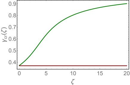
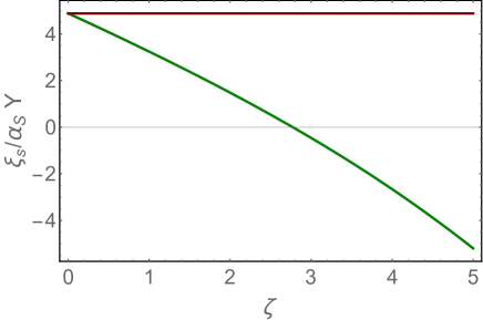
Fig. 2-a		Fig. 2-b

Figure 2: Fig. 2-a: $\gamma_{cr}$ versus $\zeta$ from Eq. (33). The red line corresponds to $\gamma_{cr}=0.37$, which is the solution of Eq. (33) at $b=0$.Fig. 2-b: $\xi_{s}\Big{/}\bar{\alpha}_{S}Y$ versus $\zeta$, where $\xi_{s}\,\,=\,\,\ln\left(Q^{2}_{s}\left(Y,\zeta\right)/Q^{2}_{s}\left(Y=0,\zeta=0\right)\right)$. The red line shows $\xi_{s}\Big{/}\bar{\alpha}_{S}Y$ at $\zeta=0$.

From Eq. (32a) we can calculate $\xi_{s}$, which is equal to

$$\xi_{s}\,\,=\,\,\ln\left(Q^{2}_{s}\left(Y,\zeta\right)/Q^{2}_{s}\left(Y=0,\zeta=0\right)\right)\,\,=\,\,-\,\frac{d\,\chi(\gamma_{\rm SP})}{d\gamma}\Big{|}_{\gamma_{\rm SP}\,=\,\gamma_{cr}\left(\zeta\right)}\,\bar{\alpha}_{S}\,Y$$ (34)

In Fig. 2-b we plot the value $\xi_{s}\Big{/}\bar{\alpha}_{S}Y$ as a function of $\zeta$. For $\zeta\,>\,2.8$, the saturation momentum starts to decrease as function of $Y$. In the vicinity of the saturation scale the scattering amplitude has the following formMUT :

$$N\left(r,b;Y\right)\,\,=\,\,N_{0}\left(r^{2}\,Q^{2}_{s}\left(Y,\zeta\right)\right)^{1\,-\,\gamma_{cr}\left(\zeta\right)}$$ (35)

where $N_{0}$ is a constant smaller than 1.

The radius of the Froissart disc ($R$) can be found from the condition:

$$N\left(r,R;Y\right)\,\,=\,\,f$$ (36)

where $f$ is a constant ( $f\,<\,1$ ). Introducing a new variable $z\,=\,\ln\left(r^{2}\,Q^{2}_{s}\left(Y,\zeta\right)\right)$, Eq. (37) can be re-written as

$$\left(1-\gamma_{cr}\left(\zeta_{R}\right)\right)\,z\,\,=\,\,\left(1-\gamma_{cr}\right)\,\left(\xi+\xi_{s}\right)\,\,=\,\,\left(1-\gamma_{cr}\right)\,\left(\xi\,-\,\,\frac{d\,\chi(\gamma_{\rm SP})}{d\gamma}\Big{|}_{\gamma_{\rm SP}\,=\,\gamma_{cr}\left(\zeta_{R}\right),\zeta=\zeta_{R}}\,\bar{\alpha}_{S}\,Y\right)=\,\,\tilde{f}$$ (37)

where $\tilde{f}\,=\,\ln\left(\frac{f}{N_{0}}\right)$. We re-write Eq. (37) as follows:

$$\eta\,\,-\,\,\frac{d\,\chi(\gamma_{\rm SP})}{d\gamma}\Big{|}_{\gamma_{\rm SP}\,=\,\gamma_{cr}\left(\zeta_{R}\right),\zeta=\zeta_{R}}\,\,=\,\,\frac{\tilde{f}}{\bar{\alpha}_{S}Y}\,\,\xrightarrow{\bar{\alpha}_{S}Y\,\gg\,1}0;~{}~{}~{}~{}~{}~{}~{}~{}~{}\eta\,\,=\,\,\frac{\xi}{\bar{\alpha}_{S}Y}$$ (38)

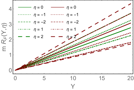
Fig. 3-a		Fig. 3-b

Figure 3: Fig. 3-a: $\zeta_{R}$ versus $\eta$ from Eq. (38). Fig. 3-b: The radius of the Froissart disc versus $Y$ at different values of $\eta$.The red lines show the estimates from Eq. (42) for the radius of the Froissart disc. The value of $\bar{\alpha}_{S}$ is taken $\bar{\alpha}_{S}=0.2$.

In Fig. 3 we plot the solution to Eq. (38) as a function of $\eta$, while in Fig. 3-b we see the dependence of the radius of the Froissart disc on $Y$. Note that the radius increases as ${\rm Const}\,Y$, but the value of ${\rm Const}$ depends on $\xi$($\eta$).

III.5 Discussion

Hence, we can conclude that in non-abelian gauge theories with the Higgs mechanism for mass generation, in the CGC approach, we obtain a Froissart disc with the radius $R\,\propto\,Y$, with a coefficient of proportionality, which depends on the size of colliding dipole.

III.5.1 Restoration of the Froissart theorem

It is easy to demonstrate the restoration of the Froissart theoremFROI for this approach. Using the unitarity constraints that $N\left(r,b;Y\right)\,\,\leq\,\,1$ , we can find the bound for the total cross section (see for example appendix 2.2 of Ref.KOLEB ):

$$\sigma_{tot}\,\,=\,\,2\int N\left(r,b;Y\right)d^{2}b\,\,<\,\,\underbrace{2\int^{b_{0}}d^{2}b}_{\mbox{unitarity constrants}}\,\,+\,\,\int_{b_{0}}d^{2}b\,\,N\left(r,b;Y\right)$$ (39)

We estimate the value of $b_{0}$, using the following equation

$$N\left(r,b_{0};Y\right)\,\,=\,\,f\,<1$$ (40)

Plugging in Eq. (40) the solution of the BFKL equation in the form: $\tilde{N}\left(r;Y\right)\,\exp\left(-\,4\,m\,b\right)$ (see Eq. (28)) we obtain

$$\tilde{N}\left(r;Y\right)\,e^{-4\,m\,b_{0}}\,\,=\,\,\underbrace{N_{0}\left(r^{2}Q_{s}(Y)\right)^{1-\gamma_{cr}}}_{\mbox{vicinity of the saturation momentum}}\,e^{-4\,m\,b_{0}}\,\,=\,\,f\,<1$$ (41)

where $\gamma_{cr}\,\,\approx\,\,0.37$ is the solution to Eq. (32a) and Eq. (32b) at $m\,=\,0$. From Eq. (41) one can see that

$$b_{0}\,\,=\,\,\frac{1}{4\,m}\Big{(}(1-\gamma_{cr})\,z\,\,-\,\,\ln\frac{f}{N_{0}}\Big{)}$$ (42)

where $z\,\,=\,\,\ln\left(r^{2}Q_{s}(Y)\right)\,\,=\,\,\xi\,\,-\,\bar{\alpha}_{S}\frac{d\chi\left(\gamma\right)}{d\,\gamma}\Big{|}_{\gamma\,=\,\gamma_{cr}}\,Y$. The dependence of the radius of the Froissart disc given by Eq. (42), is shown in Fig. 3-b by red lines. One can see that in spite of the same proportionality to $Y$, the value of the coefficients are quite different.

Plugging Eq. (42) into Eq. (39) one can see that

$$\sigma_{tot}\,\,\leq\,\,2\pi\,b^{2}_{0}\,\,=\,\,2\,\pi\left(\frac{1}{4\,m}\Big{(}\frac{1}{1-\gamma_{cr}}\,z\,\,-\,\,\ln\frac{f}{N_{0}}\Big{)}\right)^{2}$$ (43)

For $\xi=0$ Eq. (43) gives $\sigma_{tot}\,\,\leq\,\,2\,\pi\left(\bar{\alpha}_{S}\,\chi(\gamma_{cr}\,Y\right)^{2}$ and, therefore, leads to the Froissart theorem.

III.5.2 More about eigenfunctions - a recap

To learn more about the behaviour of the eigenfunction at large distances we follow Ref.LLS and consider the BFKL equation (see Eq. (11a) and Eq. (11b)) at $Q_{T}=0$. It has the form:

$$E\phi\left(\kappa\right)\,\,=$$ (44)

$$\,\,\underbrace{\frac{\kappa+1}{\sqrt{\kappa}\sqrt{\kappa+4}}\ln\frac{\sqrt{\kappa+4}+\sqrt{\kappa}}{\sqrt{\kappa+4}-\sqrt{\kappa}}\phi\left(\kappa\right)}_{{\rm kinetic\,energy\,term}}\,\,-\,\,\underbrace{\int^{\infty}_{0}\,\frac{d\kappa^{\prime}\phi\left(\kappa^{\prime}\right)}{\sqrt{(\kappa-\kappa^{\prime})^{2}\,+\,2(\kappa+\kappa^{\prime})+1}}}_{\rm potential\,energy\,term}\,\,+\,\,\underbrace{\frac{N^{2}_{c}+1}{2N^{2}_{c}}\frac{1}{\kappa+1}\int^{\infty}_{0}\frac{\phi\left(\kappa^{\prime}\right)\,d\kappa^{\prime}}{\kappa^{\prime}+1}}_{{\rm contact\,term}}$$

In Eq. (44) we introduce the following notations:

$$\kappa\,=\,\frac{q^{2}}{m^{2}};\,\,\,\,\,\,\,\,\,\,\,\,\,\,\kappa^{\prime}\,=\,\frac{q^{\prime 2}}{m^{2}};\,\,\,\,\,\,\,\,\,\,\,\,\,E\,=\,-\frac{\omega}{\bar{\alpha}_{S}};\,\,\,\,\,\,\,\,\,\,\,\,\,\bar{\alpha}_{S}\,=\,\frac{\alpha_{S}N_{c}}{\pi}$$ (45)

Re-writing Eq. (44) in the coordinate representation, we can see that it takes the form:

$$E\phi\left(r\right)\,\,=\,\,{\cal H}\,\phi\left(r\right)$$ (46)

with

$${\cal H}\,=\,\frac{\kappa^{2}+1}{|\kappa|\sqrt{\kappa^{2}+4}}\ln\frac{\sqrt{\kappa^{2}+4}+|\kappa|}{\sqrt{\kappa^{2}+4}-|\kappa|}\,\,-\,\,2K_{0}\left(|r|m\right)\,+\,\frac{N^{2}_{c}+1}{2\,N^{2}_{c}}\hat{P}\,\,=\,\,T\left(\kappa\right)\,\,+\,\,V\left(r\right)\,\,+\,\,\frac{N^{2}_{c}+1}{2\,N^{2}_{c}}\hat{P}$$ (47)

where $\hat{P}$ is a shorthand notation for the projector onto the state $\sim m^{2}/(p^{2}+m^{2})$

$$\hat{P}\,\phi\left(\kappa\right)\,=\,\frac{1}{\kappa^{2}+1}\int\frac{d^{2}\kappa^{\prime}}{\pi}\frac{\phi\left(\kappa^{\prime}\right)}{\kappa^{\prime 2}\,+\,1}$$ (48)

where $\kappa\,=\,-i\nabla_{\perp}$.

At large distances ($r\to\infty$) the potential energy in the Hamiltonian $\left(V\left(r\right)=-2K_{0}\left(rm\right)\right)$ is exponentially small, the contribution from the projector $\hat{P}$ in Eq. (46) is proportional to $1/(\kappa^{2}+1)$ and is also exponentially suppressed, so the only relevant term in the Hamiltonian is the kinetic energy

$$E\left(\kappa\right)\,\,=\,\,T\left(\kappa\right)\,\,=\,\,\frac{\kappa^{2}+1}{|\kappa|\sqrt{\kappa^{2}+4}}\ln\frac{\sqrt{\kappa^{2}+4}+|\kappa|}{\sqrt{\kappa^{2}+4}-|\kappa|},$$ (49)

for which the eigenfunctions have a form

$$\phi\left(\boldsymbol{r}\right)\,\,\sim\,\,e^{i\sqrt{\kappa^{2}}r},~{}~{}\kappa^{2}\,\,>\,\,0;\quad\phi\left(\boldsymbol{r}\right)\,\,\sim\,\,e^{-\sqrt{-\kappa^{2}}r},~{}~{}\kappa^{2}\,<\,0.$$ (50)

The point $\kappa\,=\,0$ is special, since it separates two different behaviours at large $r$. This point corresponds to energy $E=\frac{1}{2}$ or $\omega=\omega_{0}\equiv-\frac{1}{2}\bar{\alpha}_{S}$. As is shown in Ref.LLS , there are qualitative changes in the shape of the wave functions near this point. From the structure of the kinetic energy term (49) we can see that the energy $E$ is positive ($\omega<0$) for $\kappa^{2}>0$, however for $-4\,<\,\kappa^{2}\,<\,0$, the energy may have any value from $-\infty$ up to $\frac{1}{2}$. This means that for $\kappa^{2}\,<\,0$ we have a discrete spectrum with two conditions shown in Eq. (24). Hence, the exponential decrease of the eigenfunction is intimately related to the behaviour of the reggeization term in the BFKL equation, and it stems from the region, where $\omega\left(q\right)$ is positive.

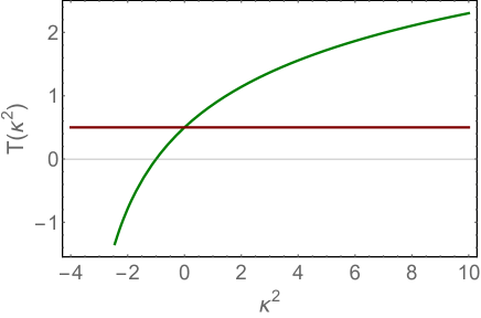
Figure 4: The dependence of the kinetic energy (see Eq. (49)) versus $\kappa^{2}$ . The red line corrsponds to $T\left(\kappa=0\right)$.

The large $b$ dependence is determined by the singularities of this term which in turn, corresponds to the singularities of the gluon propagator. In this model it is a pole at the Higgs mass. Actually, the scattering amplitude at large $b$ $N\left(r,b;Y\right)\,\xrightarrow{r\,m\,\gg\,1}\,\exp\left(-\,4\,m\,b\right)$, where $q^{2}=-4\,m^{2}$, is the singularity of the gluon reggeization in the momentum space (see Eq. (11b)). Hence, our next step will be to understand the singularities of the gluon propagator in QCD. Certainly, they have a non-perturbative origin, and we have to rely on a non-perturbative approach, which is in an embryonic stage at the moment. The only reliable information comes from lattice QCDLAT , which we will discuss in the next section.

IV Gribov - Zwanziger confinement and the BFKL equation

Among numerous approaches to confinement, the one proposed by Gribov, GRI0 ; GRI1 ; GRI2 ; GRI3 ; GRI4 ; GRREV ; DOKH ; KHLE has special advantages ,which makes it most suitable for discussion of the BFKL equation in the framework of this hypothese. First, it is based on the existence of Gribov copiesGRI0 - multiple solutions of the gauge-fixing conditions, which are the principle properties of non-perturbative QCD. Second, the main ingredient is the modified gluon propagator, which can be easily included in the BFKL-type of equations. Third, in Ref.KHLE (see also ref.FDGS ) it is demonstrated that the Gribov gluon propagator originates naturally from the topological structure of non-perturbative QCD in the form:

$$G\left(q\right)\,\,=\,\,\frac{1}{q^{2}\,\,+\,\,\frac{\chi_{\rm top}}{q^{2}}}\,\,\,=\,\,\frac{q^{2}}{q^{4}\,\,+\,\,\mu^{4}}\,\,=\,\,\frac{1}{2}\Bigg{(}\frac{1}{q^{2}\,+\,i\,\mu^{2}}\,\,+\,\,\frac{1}{q^{2}\,-\,i\,\mu^{2}}\Bigg{)}$$ (51)

where $\chi_{\rm top}\,\,=\,\,\mu^{4}$ is the topological susceptibility of QCD, which is related to the $\eta^{\prime}$ mass by the Witten-Veneziano relationVEN ; WIT . This allows us to obtain the principal non-perturbative dimensional scale, directly from the experimental data.

IV.1 The gluon propagator.

As we have discussed above, to find the large impact parameter behaviour, we need to know the gluon reggeization contribution in coordinate space. However, before calculating it, we evaluate the behaviour of the gluon propagator. As we can see from Fig. 1, the gluon reggeization term comes from the exchange of gluons at high energy. It is known (see Ref.KOLEB ) that $t$-channel gluons in the BFKL equation depend only on transverse momenta of the gluons. Hence, we need to calculate the following integral in coordinate space:

$$G\left(r\right)\,\,\,=\,\,\,\int\frac{d^{2}q_{T}}{(2\,\pi)^{2}}e^{i\boldsymbol{r}\cdot\boldsymbol{q}_{T}}\,G\left(q_{T}\right)$$ (52)

Plugging in Eq. (52) Eq. (51) we obtain

$$G\left(r\right)\,\,\,=\,\,\,\int\frac{d^{2}q_{T}}{(2\,\pi)^{2}}e^{i\boldsymbol{r}\cdot\boldsymbol{q}_{T}}\,\frac{q^{2}_{T}}{q^{4}_{T}\,\,+\,\,\mu^{2}}\,\,=\,\frac{1}{4}G_{0,4}^{3,0}\left(\frac{r^{4}\mu^{4}}{256}|\begin{array}[]{c}0,0,\frac{1}{2},\frac{1}{2}\\ \end{array}\right)$$ (53)

Where $G_{0,4}^{3,0}$ is the Meijer’s G-Function (see formulae 9.3 given in Ref.RY ).

$$G\left(r\right)\,\,\rightarrow\,\,\left\{\begin{array}[]{l l}r\,\rightarrow\infty&\,\,\,\propto~{}~{}e^{-\frac{\mu\,r}{\sqrt{2}}}\,\cos\left(\frac{\mu\,r}{\sqrt{2}}\,\,\frac{\pi}{8}\right)\\ &\\ r\,\rightarrow\,\,0&\,\,\,\propto\,~{}~{}-\ln\left(\frac{\mu\,r}{\sqrt{2}}\right)\,-\,C\end{array}\right.$$ (54)

where $C$ denotes the Euler constant.

Hence, we see that at large values of $r$ the gluon propagator decreases exponentially, giving us hope, that Gribov’s confinement will lead to a scattering amplitude, that will be exponentially small at long distances.

IV.2 The gluon trajectory.

The general expression for the gluon trajectory has the following formFKL :

$$\omega_{G}\left(q\right)\,\,=\,\,G^{-1}\left(q\right)\Sigma\left(q\right)~{}~{}~{}\mbox{where}~{}~{}\Sigma\left(q\right)\,\,=\,\,\int\frac{d^{2}q^{\prime}}{4\,\pi}G\left(\boldsymbol{q}^{\prime}\right)\,G\left(\boldsymbol{q}-\boldsymbol{q}^{\prime}\right)$$ (55)

Before making estimates with the gluon propagator of Eq. (51), we need to mention, that the lattice calculation of the gluon propagator leads to $G\left(0\right)\,\neq\,0$( see Refs.DOS ; DOV ; CDMV and references therein), in explicit contradiction with Eq. (11b). However, in Ref.DSVV ; DGSVV ; DSV it is proven that Gribov’s copies generate the gluon propagator in a more general form:

$$G\left(q\right)\,\,=\,\,\frac{q^{2}\,\,+\,\,M^{2}_{0}}{\left(q^{2}\,+\,M^{2}\right)^{2}\,\,+\,\,\mu^{4}}$$ (56)

which leads to $G\left(0\right)\,\neq\,\,0$. We consider this form as a parameterization of the sum of Gribov’s propagators of Eq. (51), with different values of $\mu$. In particular, in Ref.DKEL it was demonstrated that the approach, suggested in Ref.KHLE , leads to a gluon propagator of the following form:

$$G\left(q\right)\,=\,\frac{1}{\sqrt{\pi}}\,\frac{1}{q^{2}}\,\int^{\infty}_{0}d\zeta\,e^{-\zeta}\,\frac{\zeta^{-\frac{1}{2}}}{1\,+\,\zeta\,z}\,\,=\,\frac{\sqrt{\pi}}{\mu^{2}}\,e^{1/z}\,{\rm Erfc}\left(\frac{1}{\sqrt{z}}\right)\rightarrow\,\,\left\{\begin{array}[]{l l}\,\,\,q^{2}\,\gg\,\mu^{2}&\propto\,\,\,1/q^{2};\\ &\\ q^{2}\,\ll\,\mu^{2}&\propto\,\,\sqrt{\pi}/\mu^{2};\end{array}\right.$$ (57)

where $z\,=\,\frac{\mu^{4}}{q^{4}}$.

As we have mentioned, at high energies $q$ is a two dimensional vector, which corresponds to transverse momentum carried by the gluon. Introducing

$$G^{\pm}\left(q\right)\,\,=\,\,\frac{1}{\left(q^{2}\,\,+\,\,M^{2}\right)\,\,\pm\,i\,\mu^{2}}$$ (58)

we can re-write Eq. (56) in the form:

$$G\left(q\right)\,\,=$$ (59)

$$,\,\frac{1}{2}\Big{(}G^{+}\left(q\right)\,\,+\,\,G^{-}\left(q\right)\Big{)}\,\,+\,\,\frac{M^{2}_{0}-M^{2}}{2\,\mu^{2}\,i}\Big{(}G^{+}\left(q\right)\,\,-\,\,G^{-}\left(q\right)\Big{)}\,\,=\,\,\frac{1}{\mu^{2}}\Big{(}{\rm Re}\,G^{+}\left(\kappa\right)\,\,+\,\,(M^{2}_{0}-M^{2})\,{\rm Im}\,G^{+}\left(\kappa\right)\Big{)}$$

$$=\frac{1}{2}\Bigg{\{}(1\,\,+\,\,i\,\frac{M^{2}_{0}-M^{2}}{\mu^{2}})\,G^{+}\left(q\right)+(1\,\,-\,\,i\,\frac{M^{2}_{0}-M^{2}}{\mu^{2}})\,G^{-}\left(q\right)\Bigg{\}}=\frac{1}{2}\Bigg{\{}(1\,\,+\,\,i\,m_{0})\,G^{+}\left(\kappa\right)\,\,+\,\,(1\,\,-\,\,i\,m_{0})\,G^{-}\left(\kappa\right)\Bigg{\}}$$

where we use notation similar to Eq. (45):

$$\kappa\,=\,\frac{q^{2}}{\mu^{2}};\,\,\,\,\,\,\,\,\,\,\,\,\,\,\kappa^{\prime}\,=\,\frac{q^{\prime 2}}{\mu^{2}};\,\,\,\,\,\,\,\,\,\,\,\,\,E\,=\,-\frac{\omega}{\bar{\alpha}_{S}};\,\,\,\,\bar{\alpha}_{S}\,=\,\frac{\alpha_{S}N_{c}}{\pi};\,\,\,m\,\,=\,\,\frac{M^{2}}{\mu^{2}};\,\,\,m_{0}\,\,=\,\,\frac{M^{2}_{0}\,-\,M^{2}}{\mu^{2}};$$ (60)

Plugging Eq. (59) into Eq. (55) one can see that

$$\Sigma\left(\kappa\right)\,\,=\,\,\int\frac{d^{2}\kappa^{\prime}}{4\,\pi}\sum_{j=\pm,\,l=\pm}a_{jl}\,G^{j}\left(\boldsymbol{\kappa}^{\prime}\right)G^{l}\left(\boldsymbol{\kappa}\,-\,\boldsymbol{\kappa}^{\prime}\right)$$ (61)

where the coefficient $a_{jl}$ can be easily calculated from the decomposition of Eq. (59). Each term of Eq. (61) can be re-written in the form

$$\Sigma_{1,2}\left(\kappa\right)\,\,=\,\,\int\frac{d^{2}\kappa^{\prime}}{4\,\pi}\,G^{1}\left(\boldsymbol{\kappa}^{\prime}\right)G^{2}\left(\boldsymbol{\kappa}\,-\,\boldsymbol{\kappa}^{\prime}\right)\,\,=\,\,\int\frac{d^{2}\kappa^{\prime}}{4\,\pi}\frac{1}{(\kappa^{\prime 2}\,+\,m^{2}_{1})\,((\boldsymbol{\kappa}\,-\,\boldsymbol{\kappa}^{\prime})^{2}\,+\,m^{2}_{2})}$$ (62)

$$=\frac{1}{2}\int^{1}_{0}d\alpha\int\frac{d\kappa^{\prime 2}}{\left((\boldsymbol{\kappa}^{\prime}-\alpha\,\boldsymbol{\kappa})^{2}\,+\,\kappa\,\alpha(1-\alpha)\,\,+\,m^{2}_{1}\,-\,(m^{2}_{2}\,-\,m^{2}_{1})\alpha\right)^{2}}\,\,=\,\,\frac{1}{2}\int^{1}_{0}d\alpha\frac{1}{\,\kappa\,\alpha(1-\alpha)\,+\,m^{2}_{1}\,-\,(m^{2}_{2}\,-\,m^{2}_{1})\alpha}$$

where we have introduced the Feyman parameter $\alpha$ and $m^{2}_{1}=\,m\,\pm i$ and $m^{2}_{2}\,=\,m\,\pm\,i$.

Integrating over $\alpha$ we obtain:

$$\Sigma_{1,2}\,=\,\frac{1}{\Delta}\displaystyle{\Big{\{}\ln\Big{(}\frac{-\kappa\,+\,m^{2}_{2}\,-\,m^{2}_{1}\,+\,\Delta}{\kappa\,+\,m^{2}_{2}\,-\,m^{2}_{1}\,+\,\Delta}\Big{)}\,\,\,-\,\,\ln\Big{(}\frac{\kappa\,-\,m^{2}_{2}\,+\,m^{2}_{1}\,+\,\Delta}{-\kappa\,-\,m^{2}_{2}\,+\,m^{2}_{1}\,+\,\Delta}\Big{)}}\Big{\}}$$ (63)

where $\Delta\,\,=\,\,\sqrt{-\left(\kappa+(m_{1}-m_{2})^{2}\right)\,\left(\kappa\,+\,(m_{1}\,+\,m_{2})^{2}\right)}$ and $\kappa$ is defined in Eq. (45).

Cumbersome, but simple calculations lead from Eq. (63) to the expression for the gluon trajectory $T\left(\kappa\right)\,\,=\,\,2\,\Omega_{G}\left(\kappa\right)$ (see appendix A). Fig. 5-a shows the resulting $T(\kappa)$ as function of $\kappa$ for different values of $m$ and $m_{0}$.

At first sight, the behaviour of the kinetic energy (see Fig. 5 ) for the BFKL with Gribov’s confinement, is not that different from the case that we have described in section III. Indeed, $T$ is negative for negative $\kappa$ ( see Fig. 5-a), and due to this, we expect we have a bound state as in the case of the model, discussed in section III. As in the model of section III for negative $\kappa$, we expect the eigenfunction, which is small at large $r$ ($\Psi\,\propto\,\exp\left(-\sqrt{|\kappa|}\,r\right)$). Hence, we expect that the scattering amplitude will decrease at large $b$. For example, we see such a situation in Fig. 5-b, where the kinetic energy is plotted for the gluon propagator, which is in agreement with lattice QCD data DOS . However, the actual setup is more interesting: for the propagator of Eq. (51), the kinetic energy is positive for all values of $\kappa$ (see Fig. 6). We will argue below that in this case, the generalized BFKL Pomeron has the intercept which is equal to zero, and the eigenfunctions do not decrease exponentially at large $r$.

In the appendix A we discuss the $\kappa$ dependence of $\omega_{G}$ in more detail.

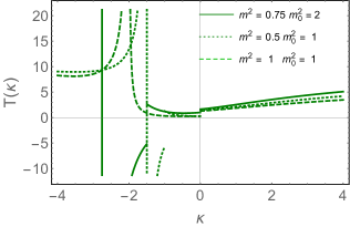
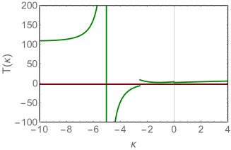
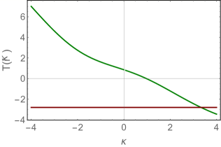
Fig. 5-a	Fig. 5-b	Fig. 5-c

Figure 5: Fig. 5-a: $T\left(\kappa\right)$ versus $\kappa$ at different values of $m$ and $m_{0}$.Fig. 5-b: The same as Fig. 5-a but for $m_{0}=5.03$ , $m=1.27$ and $\mu^{2}=0.459\,GeV^{2}$, which corresponds to the description of recent calculations in lattice QCD(DOS , section 2.1). In Fig. 5-c the kinetic energy $T\left(i\,\kappa\right)$ is plotted. The red line corresponds to $T\left(\kappa\right)=-\Delta_{\rm BFKL}\,\,=\,\,-4\ln 2$, where $\Delta_{\rm BFKL}$ is the intercept of the BFKL Pomeron for QCD.

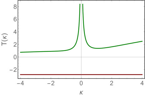
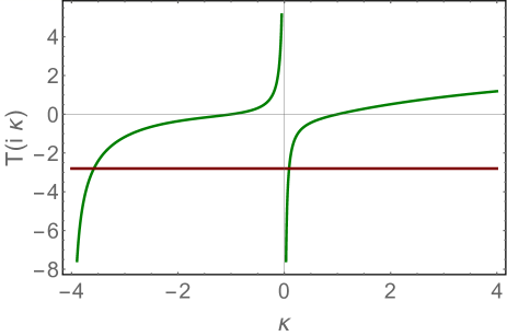
Fig. 6-a		Fig. 6-b

Figure 6: $\omega_{G}\left(\kappa\right)$ versus $\kappa$ for the Gribov propagator of Eq. (51). The red line corresponds to $T\left(\kappa\right)=-\Delta_{\rm BFKL}\,\,=\,\,-4\ln 2$, where $\Delta_{\rm BFKL}$ is the intercept of the BFKL Pomeron for QCD. Fig. 6-a: $T\left(\kappa\right)$, Fig. 6-b:$T\left(i\,\kappa\right)$.

IV.3 The BFKL equation in momentum representation.

In the previous section we found $\omega_{G}\left(q\right)$, now we are going to find the kernel which is responsible for gluon emission. Using the decomposition of Eq. (51) for the Gribov propagator, we can treat the production of the gluon as sum of two sets of the diagrams (see Fig. 7 ) with $\tilde{M}^{2}=\,\,i\mu^{2}$ and with $\tilde{M}^{2}=-\,\,i\mu^{2}$.

We sum the first diagrams of the gluon emission shown in Fig. 7 to find the vertex $\Gamma_{\mu}\left(q,q^{\prime}\right)$ for the kernel of the BFKL equation (see Fig. 1-b). It is easy to see that the sum shown in Fig. 7, leads to the Lipatov vertex that has the following form

$$\Gamma_{\mu}\left(q,q^{\prime}\right)\,\,=\,\,-q^{\perp}_{\mu}\,-\,q^{\prime\perp}_{\mu}\,+\,p_{1,\mu}\left(-G^{-1}\left(q\right)\frac{1}{p_{1}\cdot k}\,+\,\frac{p_{2}\cdot k}{p_{1}\cdot p_{2}}\right)\,-\,p_{2,\mu}\left(-G^{-1}\left(q^{\prime}\right)\frac{1}{p_{2}\cdot k}\,+\,\frac{p_{1}\cdot k}{p_{1}\cdot p_{2}}\right)$$ (64)

The gluon production vertex for the conjugated reggeized gluon can be written as follows

$$\tilde{\Gamma}_{\mu}\left(q_{1},q_{1}^{\prime}\right)\,\,=\,\,-q^{\perp}_{1,\mu}\,-\,q^{\prime\perp}_{1,\mu}\,+\,p_{1,\mu}\left(-G^{-1}\left(q_{1}\right)\frac{1}{p_{1}\cdot k}\,+\,\frac{p_{2}\cdot k}{p_{1}\cdot p_{2}}\right)\,-\,p_{2,\mu}\left(-G^{-1}\left(q^{\prime}_{1}\right)\frac{1}{p_{2}\cdot k}\,+\,\frac{p_{1}\cdot k}{p_{1}\cdot p_{2}}\right)$$ (65)

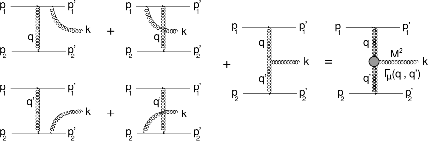
Figure 7: The first Feynman diagrams with gluon emission, whose sum leads to $\Gamma_{\nu}\left(q,q^{\prime}\right)$ (Lipatov vertex is denoted by the gray blob ).

The BFKL kernel for one given configuration of the masses ( say, $\tilde{M^{2}}\,=\,+i\,\mu^{2}$) at $Q_{T}=0$ ( for forward scattering $q=q_{1},q^{\prime}=q^{\prime}_{1}$) is given by

$$\left(G^{-1}\left(q^{\prime}\right)\right)^{2}K\left(q,q^{\prime}\right)\,=\,\Gamma_{\mu}\left(q,q^{\prime}\right)\cdot\tilde{\Gamma}_{\mu}\left(q,q^{\prime}\right)\,=\\ \,\,\underbrace{4\Bigg{(}\frac{G^{-1}\left(q\right)\,G^{-1}\left(q^{\prime}\right)}{k^{2}+\tilde{M}^{2}}\Bigg{)}}_{\mbox{gluon emission}}\,\,-\,\,\underbrace{2\,M^{2}\left(\frac{N^{2}+1}{N^{2}_{c}}\right)}_{\mbox{contact term}}$$ (66)

where the contact term has been discussed in Ref.LLS and $K\left(q,q^{\prime}\right)$ is the BFKL kernel of gluon emission. $N_{c}$ in Eq. (66) denotes the number of colours.

Illustrating the derivation of Eq. (66), we calculate the diagram with the emission of one gluon in quark-antiquark scattering, to understand the structure of the BFKL equation (see Fig. 7). The contribution of this diagram is equal to

$$N\left({Fig.~{}\ref{3}}\right)\,=\,\frac{\alpha_{S}N_{c}}{2\pi^{2}}\int d^{2}q\,d^{2}q^{\prime}\,G^{2}\left(q\right)\,\Gamma_{\mu}\left(q,q^{\prime}\right)\cdot\tilde{\Gamma}_{\mu}\left(q,q^{\prime}\right)\,G^{2}\left(q^{\prime}\right)$$

The gluon emission term can be re-written in the simple form

$$N_{\mbox{gluon emission}}\left({Fig.~{}\ref{3}}\right)\,\,=\,\,\frac{\alpha_{S}N_{c}}{2\pi^{2}}\int d^{2}q\,d^{2}q^{\prime}\,G\left(q\right)\,G\left(k\right)G\left(q^{\prime}\right)$$ (67)

Collecting all terms, including the gluon reggeization, which has been discussed in the previous section, and summing the contributions with $M^{2}$ and $\tilde{M}^{2}$, we obtain the BFKL equation in the form:

$$\omega\,\phi\left(\omega,q\right)\,\,=\,\,-\,2\omega_{G}\left(q\right)\,\,\phi\left(\omega,q\right)\,\,+\,\,\bar{\alpha}_{S}\int\frac{d^{2}q^{\prime}}{\pi}G\left(\boldsymbol{q}-\boldsymbol{q}^{\,{}^{\prime}}\right)\,\,\phi\left(\omega,q^{\prime}\right)$$ (68)

Assuming that $\phi\left(q\right)$ depends only on $|\boldsymbol{q}|$, we can integrate the emission kernel over the angle and in terms of the variable of Eq. (60), Eq. (68) takes the form:

$$E\,\phi\left(\kappa\right)\,\,=\,\,\,T\left(\kappa\right)\,\,-\,\,\int d\kappa^{\prime}\,K\left(\kappa,\kappa^{\prime}\right)\,\phi\left(\kappa^{\prime}\right)\,\,\,$$ (69)

where

$$K\left(\kappa,\kappa^{\prime}\right)\,\,\,=\,\,\,\displaystyle{{\rm Re}\Bigg{\{}\frac{1\,+\,i\,m_{0}}{\sqrt{2(m+i)(\kappa\,\,+\,\,\kappa^{\prime})+(m+i)^{2}+(\kappa\,-\,\kappa^{\prime})^{2}}}\Bigg{\}}}$$ (70)

and

$$G\left(\kappa\right)\,\,=\,\,\frac{\kappa\,+\,m\,+\,m_{0}}{\left(\kappa\,+\,m\right)^{2}\,\,+\,\,1};~{}~{}~{}~{}\kappa\,=\,q^{2}/\mu^{2}$$ (71)

In Eq. (69) - Eq. (71) we introduce $m$ and $m_{0}$, which are equal to $m^{2}/\mu^{2}$ and $m^{2}_{0}/\mu^{2}$, respectively (see Eq. (60)).

This equation appears to be similar to the BFKL equation for a massive gluon (see Ref. LLS , and section III) in the non-abelian Yang-Mills theories with a Higgs particle, which is responsible for generation of mass. However, we do not have a contact term in Eq. (68), which stems in such an approach from the mass of the gluon and from Higgs production. It is instructive to note, that for the Gribov’s propagator the contact term does not appear, even if we assume the existence of a Higgs meson, with mass squared $\pm i\mu^{2}$. A more general form of the gluon propagator, which is given in Eq. (56) and which we view as a sum of Gribov’s propagators, also does not generate a contact term. Therefore, the absence of a contact term in our equation, is a direct indication that Gribov-Zwanziger confinement does not lead to a massive gluon.

IV.4 The Pomeron intercept.

IV.4.1 General features of the equation’s spectrum

Following the general pattern of Ref.LLS we can re-write Eq. (69) in the form of Eq. (44) -Eq. (48) (see section IIIE.2):

$$E\,\Psi\left(r\right)\,\,=\,\,{\cal H}\,\Psi\left(r\right)$$ (72)

with

$${\cal H}\,\,=\,\,T\left(\hat{\kappa}\right)\,\,-\,\,G\left(r\right)\,\,+\,\,\frac{N^{2}_{c}+1}{2\,N^{2}_{c}}\hat{P}$$ (73)

where $\sqrt{\hat{\kappa}}\,\,=\,\,-\,i\boldsymbol{\nabla}_{\perp}$ and $\hat{P}$ is a shorthand notation for the projector onto the state $\sim m^{2}/(p^{2}+m^{2})$

$$\hat{P}\,\phi\left(p\right)\,=\,2m^{2}G\left(\kappa\right)\int d\kappa^{\prime}G\left(\kappa^{\prime}\right)\phi\left(\kappa^{\prime}\right)\,\,\xrightarrow{\rm coordinate\,\,image}G\left(r\right)\,C_{1}~{}~{}~{}\mbox{where}~{}~{}C_{1}\,=\,2m^{2}\int d\kappa^{\prime}G\left(\kappa^{\prime}\right)\phi\left(\kappa^{\prime}\right)$$ (74)

For large $r$, $G\left(r\right)$ exponentially decreases (see Eq. (54)) as well as the contact term. Hence, at large $r$ Eq. (72) takes the following form:

$$E\Psi\left(r\right)\,\,=\,\,T\left(\hat{\kappa}\right)\Psi\left(r\right)$$ (75)

with the eigenfunctions of Eq. (50). Denoting the large asymptotic behaviour of the eigenfunction as $\Psi\left(r\right)\xrightarrow{r\,\gg\,\,1/\mu}\,\,\exp\left(-\sqrt{a}\,r\right)$, we see that the energy is equal to

$$E\,\,=\,\,T\left(-\,a\right)$$ (76)

On the other hand, it is shown in Ref.LLS (see section III-D) that in the region of small $r$ Eq. (73) reduces to the massless QCD BFKL equation FKL ; BFKL ; LIP :

$$E\,\Psi\left(r\right)\,\,=\,\,{\cal H}_{0}\,\Psi\left(r\right)$$ (77)

whereLIP

$${\cal H}_{0}\,=\,\ln p^{2}\,+\,\ln|r|^{2}\,-\,2\psi\left(1\right)\,$$ (78)

The eigenfunctions of Eq. (77) are $\Psi\left(r\right)\,=\,r^{2(1-\gamma)}$, and the eigenvalues of Eq. (77) can be parametrized as a function of $\gamma$ (see Eq. (• ‣ III.3)). Therefore, for $r\,\to\,0$ we have the eigenvalue which is equal to

$$E\,\,\,=\,\,\chi\left(\gamma\right)$$ (79)

From Eq. (76) and Eq. (79) we can conclude, that the value of $a$ and $\gamma$ are correlated, since

$$E\,\,\,=\,\,\chi\left(\gamma\right)\,\,=\,\,T\left(-\,a\right)$$ (80)

Based on Eq. (80) we expect that the minimum eigenvalue is equal to $\chi(\frac{1}{2})\,=\,-\,4\,\ln 2$. For the simplest Gribov’s propagator of Eq. (51) we see from Fig. 6 that $T\left(\kappa\right)\,>\,0$ for all values of $-\infty\,<\,\kappa\,<\,+\infty$ which means that $\gamma$ in Eq. (80), should be such that $\chi\left(\gamma\right)>0$. Consequently, we infer that Eq. (80) contradicts Eq. (79).

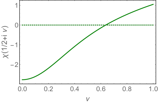
Figure 8: The eigenvalues of the BFKL equation for QCD $E\,=\,\chi(\gamma)$ versus $\gamma=\frac{1}{2}\,+\,i\,\nu$. The solid line shows the real part of E, while the dotted line shows the imaginary part.

A possible way out of this contradiction, could be that both equations are correct for specific values of $\gamma$. In Fig. 8 we plot the eigenvalues of the massless BFKL equation for $\gamma=\frac{1}{2}\,+\,i\,\nu$. One can see that for $\nu\,\geq\,0.6$ the energy is positive. Hence, this value of $\nu$ could correspond to the Pomeron with the intercept which is equal to zero. The fact that the so called soft Pomeron has a small intercept, is one of the reliable results of the high energy phenomenological attempt to describe the soft data at the LHC.

However, for $m\,\neq\,0$ and $m_{0}\,\neq\,0$ the kinetic energy could be negative, and Eq. (80) holds for $\gamma=\frac{1}{2}$, leading to the intercept of the Pomeron which coincides with the intercept of the massless BFKL Pomeron. In particular, this is the case for the gluon propagator which describes the lattice QCD data ( see Ref.DOS and Fig. 5-b).

IV.4.2 Estimates from the variational method

As we have discussed above, we expect that (1) the energy of the ground state will be close to zero for $m\,=\,0$ and $m_{0}\,=\,0$; and (2) it will be the same as for the massless BFKL equation, for $m^{2}\,\neq\,0$ and $m^{2}_{0}\,\neq\,0$ . In this section we check this, using the variational approach. In this approach, the upper bound for the ground state energy $E_{0}$ of the Hamiltonian $\mathcal{H}$ may be found by minimizing the functional

$$E_{\mbox{ground}}\,\,\equiv\,\,E_{0}\,\,\,\leq\,\,\,F[\{\phi\}]\,\,=\,\,\frac{\Big{\langle}\phi^{\ast}\!\left(r\right)\Big{|}{\cal H}\Big{|}\phi\!\left(r\right)\Big{\rangle}}{\Big{\langle}\phi^{\ast}\!\left(r\right)\Big{|}\phi\!\left(r\right)\Big{\rangle}}$$ (81)

Eq. (81) means that the functional $F[\{\phi\}]$ has a minimum for the function $\phi_{0}\left(r\right)$, which is the eigenfunction of the ground state with energy $E_{0}$.

For our Hamiltonian in momentum space, Eq. (81) can be re-written in the form

$$E_{0}\,\,=$$ (82)

$$\min_{\phi}\left\{\frac{\int^{\infty}_{0}d\kappa\,T\left(\kappa\right)\,|\phi\left(\kappa\right)|^{2}\,-\,\int^{\infty}_{0}d\kappa\int^{\infty}_{0}d\kappa^{\prime}\,K\left(\kappa,\kappa^{\prime}\right)\,\phi\left(\kappa\right)\phi^{*}\left(\kappa^{\prime}\right)\,\,+\,2m\frac{N^{2}_{c}+1}{2N^{2}_{c}}\Big{|}\int^{\infty}_{0}d\kappa\,\frac{\phi\left(\kappa\right)}{\kappa+1}\Big{|}^{2}}{\int^{\infty}_{0}d\kappa|\phi\left(\kappa\right)|^{2}}\right\}$$

The success of finding the value of $E_{0}$, depends on the choice of the trial functions in Eq. (82). We choose it in the form

$$\phi_{\mbox{trial}}\left(\kappa\right)\,\,=\,\,\left(\frac{\kappa}{\kappa^{2}+a^{2}}\right)^{\gamma}$$ (83)

In the coordinate representation Eq. (83) corresponds to

$$\Psi_{\mbox{trial}}\left(r\right)\,\, = \,\,2^{-2(\gamma+2)}\left(\frac{1}{a^{4}}\right)^{-\gamma}\left(a^{4}\right)^{-\gamma}\left(\frac{\sqrt{\pi}2^{\gamma+3}\left(\frac{1}{a^{4}}\right)^{\frac{\gamma-1}{2}}\Gamma\left(\frac{\gamma-1}{2}\right)\,_{1}F_{4}\left(\frac{\gamma}{2}+\frac{1}{2};\frac{1}{2},\frac{1}{2},1,\frac{3}{2}-\frac{\gamma}{2};-\frac{1}{256}a^{4}r^{4}\right)}{\Gamma\left(\frac{\gamma}{2}\right)}\right.$$ (88)

$$\left.+\frac{32\Gamma(1-\gamma)r^{2\gamma-2}\,_{1}F_{4}\left(\gamma;\frac{\gamma}{2}+\frac{1}{2},\frac{\gamma}{2}+\frac{1}{2},\frac{\gamma}{2},\frac{\gamma}{2};-\frac{1}{256}a^{4}r^{4}\right)}{\Gamma(\gamma)}\right.$$

$$\left.-\frac{\sqrt{\pi}2^{\gamma}\gamma r^{2}\left(\frac{1}{a^{4}}\right)^{\frac{\gamma}{2}-1}\Gamma\left(\frac{\gamma}{2}-1\right)\,_{1}F_{4}\left(\frac{\gamma}{2}+1;1,\frac{3}{2},\frac{3}{2},2-\frac{\gamma}{2};-\frac{1}{256}a^{4}r^{4}\right)}{\Gamma\left(\frac{\gamma+1}{2}\right)}\right)$$

$$\rightarrow\,\,\left\{\begin{array}[]{l l}r\,\rightarrow\infty&\,\,\,\propto~{}~{}r^{-2(\gamma+1)}\\ &\\ r\,\rightarrow\,\,0&\,\,\,\propto\,~{}~{}r^{-2+2\gamma}\end{array}\right.$$

The form of the trial function was suggested by the form of Gribov’s propagator. One can see that our trial function has the expected behaviour for the case of $m=0,m_{0}=0$ , if $a>0$ and $b\,=\,2\gamma-1\,>\,0$, leading to a power-like decrease at large $r$. Such a function cannot be an eigenfunction of ${\cal H}=T(\kappa)$, indicating possible difficulties with Eq. (80).

In Fig. 9-a and Eq. (9)-b we calculate $E_{\mbox{ground}}$ from Eq. (81), for the case of Gribov’s propagator of Eq. (51) ($m=0,m_{0}=0$). In appendix B we describe the details of the numerical estimates.

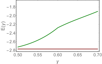
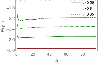
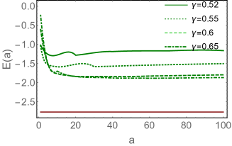
Fig. 9-a	Fig. 9-b	Fig. 9-c

Figure 9: Fig. 9-a: $E\equiv-{\rm Pomeron\,\,intercept}$ of the BFKL Pomeron versus $\gamma$ at different values of $\gamma$ for $a=100$ and $m=0$ and $m_{0}=0$. These values of $m$ and $m_{0}$ correspond to the Gribov’s propagator of Eq. (51), which stems from Refs.GRI0 ; GRI1 ; GRI2 ; GRI3 ; GRI4 . Fig. 9-b: The same as in Fig. 9-a but at fixed values of $\gamma$ as function of $a$. In Fig. 9-c we plot the energy as function of $a$ for the case of $m=1.27\mu^{2}$ and $m_{0}=3.76\mu^{2}$ , which describes the lattice QCD evaluation of the gluon propagator DOS . The estimates for $E$ were performed in the framework of the variational method with the trial function $\phi_{\rm trial}$ of Eq. (83) (see appendix B for details).

We obtain the minimal energy corresponds to $\gamma\,=\,\frac{1}{2}$ in accord with our expectation. However, $E_{\mbox{ground}}\,\,\to\,\,-4\ln 2$ instead of $E_{\mbox{ground}}=0$, in contradiction to our expectations. Note that the singularities of the trial function corresponds to $\kappa\,=\,i\,a$. In Fig. 6-c we plot the kinetic energy at pure imaginary $\kappa$, and we see that $T\left(i\kappa\right)$ can be negative and equal to $-4\,\ln 2$.

For $m^{2}\,\neq\,0$ and $m^{2}_{0}\,\neq\,0$ we face a different problem: $\gamma$ turns out to be larger than expected $\gamma=\frac{1}{2}$, and the energy level is far away from the ground state energy $E=-4\ln 2$ for the massless BFKL equation(see Fig. 9-c). Perhaps, this result is due to our choice of the trial function, not being satisfactory. We believe, that both observations show that we need to solve Eq. (69) numerically, in the same way as it has been done in Ref.LLS . We intend to do this in the near future, and we will publish the results elsewhere.

IV.5 The BFKL kernel in the coordinate representation.

Using Eq. (12), and the decomposition of Eq. (59), we obtain the gluon propagator of Eq. (56) in the coordinate representation in the form:

$$G\left(r\right)\,\,\,=\,\,\,\frac{1}{2}\left(\left(1-\frac{\text{m}_{0}^{2}}{i}\right)K_{0}\left(r\,\sqrt{m^{2}-i}\right)+\left(1+\frac{\text{m}^{2}_{0}}{i}\right)K_{0}\left(r\,\sqrt{m^{2}+i}\right)\right)$$ (89)

Note, that we now return to using the notation $m=M/\mu$ and $m_{0}=\sqrt{M^{2}_{0}\,-\,M^{2}}/\mu$ .

At large $r$ it tends to

$$G\left(r\right) \,\,\xrightarrow{\mu\,r\,\gg\,\,1} \frac{1}{2}\sqrt{\frac{\pi}{2\,\,r}}{\rm Re}\left(\frac{\left(1-i\text{m}^{2}_{0}\right)e^{-\,r\,\sqrt{m^{2}+i}}}{\sqrt[4]{m^{2}+i}}\right)$$

$$= \frac{1}{2}\sqrt{\frac{\pi}{2\,\,r}}e^{-r\sqrt{m^{2}\,+\,1}\cos\theta}\Bigg{(}\cos\left(-r\sqrt{m^{2}\,+\,1}\sin\theta+\frac{1}{2}\theta\right)-\,m^{2}_{0}\sin\left(-r\sqrt{m^{2}\,+\,1}\sin\theta+\frac{1}{2}\theta\right)\Bigg{)}$$

where

$$\cos\theta\,\,=\,\,\sqrt{\frac{1}{2}\left(1\,\,+\,\,\frac{m}{\sqrt{m^{2}\,+\,1}}\right)};~{}~{}~{}\sin\theta\,\,=\,\,\sqrt{\frac{1}{2}\left(1\,\,-\,\,\frac{m}{\sqrt{m^{2}\,+\,1}}\right)}.$$

Hence, one can see that the gluon propagator decreases exponentially at large $r$, even at $m=0$. From Eq. (IV.5) we can conclude that

$$\Sigma\left(r\right)\,\,\,=\,\,G^{2}\left(r\right)\xrightarrow{\mu\,r\,\gg\,\,1}\Bigg{(}\frac{1}{2}\sqrt{\frac{\pi}{2\,\,r}}{\rm Re}\left(\frac{\left(1-i\text{m}^{2}_{0}\right)e^{-\sqrt{m^{2}+i}r}}{\sqrt[4]{m^{2}+i}}\right)\Bigg{)}^{2}\,\,\propto\,\,e^{-\,r\,2\sqrt{m^{2}\,+\,1}\cos\theta}$$ (91)

From Eq. (56) and $\boldsymbol{q}\,=\,-i\,\boldsymbol{\nabla}$ we conclude that $\omega_{G}\left(r\right)$ is equal to

$$\omega_{G}\left(r\right)\,\,=\,\,\int d^{2}\,r^{\prime}\,K_{0}\left(M_{0}\,|\boldsymbol{r}\,-\,\boldsymbol{r}^{\prime}|\right)\Big{(}\left(-\nabla^{2}_{r^{\prime}}\,\,+\,\,m^{2}\right)^{2}+1\Big{)}\,\Sigma\left(r^{\prime}\right)$$ (92)

In Eq. (92) the behaviour of $\omega_{G}\left(r\right)$ at large $r$ stems from the integration in two regions: $M_{0}\,|\boldsymbol{r}\,-\,\boldsymbol{r}^{\prime}|\,\leq\,1$ and $\,r^{\prime}\,2\sqrt{m^{2}\,+\,1}\cos\theta\,\leq\,1$. The first region leads to the asymptotic behaviour of Eq. (92), while the second region gives $\omega_{G}\left(r\right)\,\,\propto\,\exp\left(-M_{0}\,r\right)$. Hence for $M_{0}\,<\,2\sqrt{m^{2}\,+\,1}\cos\theta$ $\omega_{G}\left(r\right)\,\,\propto\,\exp\left(-M_{0}\,\,r\,\right)$. Lattice QCD leads to such behaviour of $\omega_{g}$, as it can be seen from Fig. 6. It should be stressed, that the exponential decrease depends on the value of the gluon propagator at $q=0$ $G\left(q=0\right)\,\,\propto\,M_{0}^{2}/\mu^{4}$. In other words, the original Gribov propagator of Eq. (51) does not give the BFKL kernel which decreases exponentially at large $b$. Indeed, at $M_{0}\,\to\,0$ instead of $\exp\left(-M_{0}\,r\right)$ decrease, we have $\ln r$ behaviour from the region $\sqrt{m^{2}+1}\,r^{\prime}\,\leq\,1$. However, even for $m_{0}\neq 0$ one can see from Eq. (51), that $\omega_{G}$ is a decreasing function, with oscillations. These oscillations do not contradict the unitarity constraints, they also do not violate the exponential decrease of the scattering amplitude at large $b$.

V Non-linear equation and the size of Froissart disc.

The eigenfunctions of the master equation (see Eq. (69)) at short distances are proportional to $\left(r^{2}\right)^{1-\gamma}$ and, therefore, for deep inelastic scattering, which occurs at short distances, the solution has the form of Eq. (31). Hence, repeating the procedure that has been discussed in Eq. (32a) - Eq. (33), we obtain the same equations for the radius of the Froissart disc (see Eq. (37) and Eq. (38)). The variable $\zeta$ takes the form: $\zeta=4(m+m_{0})b/\bar{\alpha}_{S}\,Y$. Actually, as we have discussed in section IV-E, the asymptotic exponential decrease at $r\,\geq\,1/\mu$ is determined by the smaller of the two masses: $m+m_{0}$ and $2\,\sqrt{m^{2}\,+\,\mu^{2}}$. For the realistic case of $m^{2}=1.27\mu^{2}$ and $m^{2}_{0}=3.76\,\mu$ DOS $m+m_{0}\,\,<\,\,2\,\sqrt{m^{2}\,+\,\mu^{2}}$.

The non-linear equation has the same form as Eq. (1) with the kernel

$$K\left(\boldsymbol{r}^{\prime},\boldsymbol{r}-\boldsymbol{r}^{\prime};\boldsymbol{r}\right)\,\,\,=\,\,\frac{r^{2}}{r^{\prime 2}}\int d^{2}\,r^{\prime\prime}\,K_{0}\left(M_{0}\,|\boldsymbol{r}\,-\boldsymbol{r}^{\prime}\,-\,\,\boldsymbol{r}^{\prime\prime}|\right)\Big{(}\left(-\nabla^{2}_{r^{\prime\prime}}\,\,+\,\,m^{2}\right)^{2}+1\Big{)}\,\Sigma\left(r^{\prime\prime}\right)$$ (93)

It should be noted, that this kernel approaches the kernel of Eq. (1) at short distances. Generally speaking, at $r\,\geq\,1/\mu$ (see Eq. (51)) we need to take into account the full kernel of Eq. (93). However, for DIS processes the typical $r\,\propto\,1/Q\,\,\ll\,\,1/\mu$, where $Q$ is the photon virtuality, and we can safely use the kernel of Eq. (1), even in the saturation region, where $r^{2}\,Q^{2}_{s}\left(Y,b\right)\,>\,1$. Restricting ourselves to the DIS process, we wish to consider the following $r$

$$\frac{1}{\mu^{2}}\,\,>\,\,r^{2}\,\,>\,\,\frac{1}{Q^{2}_{s}\left(Y,b\right)}$$ (94)

However, even in this region the general non-linear evolution of Eq. (1) is difficult to analyze analytically, for the full BFKL kernel of Eq. (2) . This kernel includes the summation over all twist contributions. We would like to start with a simplified version of the kernel in which we restrict ourselves to the leading twist term onlyLETU . For the leading twist term we only sum logs terms, and actually we have two types of logs: $\Big{(}\bar{\alpha}_{S}\ln\left(r\,\Lambda_{QCD}\right)\Big{)}^{n}$ in the perturbative QCD kinematic region where $r\,Q_{s}\left(Y,b\right)\,\,\equiv\,\,\tau\,\,\ll\,\,1$; and $\Big{(}\bar{\alpha}_{S}\ln\left(r\,Q_{s}\left(Y,b\right)\right)\Big{)}^{n}$ inside the saturation domain ($\tau\,\gg\,1$), where $Q_{s}\left(Y,b\right)$ denotes the saturation scale. To sum these logs it is necessary to modify the BFKL kernel in different ways in the two kinematic regions, which takes the form

$$\chi\left(\gamma\right)\,\,=\,\,\left\{\begin{array}[]{l}\,\,\,\frac{1}{\gamma}\,\,\,\,\,\,\,\,\,\,\mbox{for}\,\,\,\tau\,=\,rQ_{s}\,<\,1\,\,\,\,\,\,\mbox{summing}\left(\ln\left(1/(r\,\Lambda_{\rm QCD})\right)\right)^{n};\\ \\ \,\,\,\frac{1}{1\,-\,\gamma}\,\,\,\,\,\mbox{for}\,\,\,\tau\,=\,rQ_{s}\,>\,1\,\,\,\,\,\mbox{summing}\left(\ln\left(rQ_{s}\right)\right)^{n};\end{array}\right.$$ (98)

instead of the full expression of Eq. (2). Recall that the solution has the form of Eq. (31).

Inside the saturation region where $\tau\,\,=\,\,r^{2}\,Q^{2}_{s}\left(Y,b\right)\,\,>\,\,1$, the logs originate from the decay of a large size dipole into one small size dipole and one large size dipole. However, the size of the small dipole is still larger than $1/Q_{s}$. This observation can be translated in the following form of the kernel

$$\int\,\displaystyle{K\left(\boldsymbol{x}_{01};\boldsymbol{x}_{02},\boldsymbol{x}_{12}\right)}\,d^{2}x_{02}\,\,\rightarrow\,\pi\,\int^{x^{2}_{01}}_{1/Q^{2}_{s}(Y,b)}\frac{dx^{2}_{02}}{x_{02}^{2}}\,\,+\,\,\pi\,\int^{x^{2}_{01}}_{1/Q^{2}_{s}(Y,b)}\frac{d|\boldsymbol{x}_{01}-\boldsymbol{x}_{02}|^{2}}{|\boldsymbol{x}_{01}-\boldsymbol{x}_{02}|^{2}}$$ (99)

Inside the saturation region Eq. (1) has the form

$$\frac{\partial^{2}\widetilde{N}\left(Y;\xi,\boldsymbol{b}\right)}{\partial Y\,\partial\xi}\,\,=\,\,\bar{\alpha}_{S}\,\left\{\left(1\,\,-\,\frac{\partial\widetilde{N}\left(Y;\boldsymbol{r},\boldsymbol{b}\right)}{\partial\xi}\right)\,\widetilde{N}\left(Y;\xi,\boldsymbol{b}\right)\right\}$$ (100)

where $\widetilde{N}\left(Y;\xi,\boldsymbol{b}\right)\,\,=\,\,\int^{r^{2}}dr^{\prime 2}\,N\left(Y;\boldsymbol{r}^{\prime},\boldsymbol{b}\right)/r^{\prime 2}\,\,=\,\,\int^{\xi}d\xi^{\prime}N\left(Y,\xi^{\prime},\boldsymbol{b}\right)$ .

Rewriting $\frac{\partial}{\partial Y}$ in terms of

$$z\,\,=\,\,-\,\frac{d\,\chi\left(\gamma_{\rm SP}\right)}{d\gamma_{\rm SP}}\Big{|}_{\gamma_{\rm SP}\,\,=\,\,\gamma_{cr}\left(\zeta\right)}\,\bar{\alpha}_{S}Y\,\,+\,\,\xi\,\,\,=\,\,\lambda\left(\zeta\right)\,\bar{\alpha}_{S}\,Y\,\,+\,\,\xi;~{}~{}~{}\mbox{where}\,\,\xi\,\,=\,\,\ln\left(r^{2}\,Q^{2}_{s}\left(Y=Y_{0},b=0\right)\right)$$ (101)

we obtain

$$\frac{\partial}{\partial Y}\,=\,\frac{\partial}{\partial\,z}\frac{\partial\,z}{\partial Y}\,=\,\bar{\alpha}_{S}\Big{(}\lambda\left(\zeta\right)\,\,-\,\,\zeta\frac{d\lambda\left(\zeta\right)}{d\zeta}\Big{)}\frac{d}{d\,z}\,\,\equiv\,\,\bar{\alpha}_{S}\,\kappa\left(\zeta\right)\,\frac{d}{d\,z}$$ (102)

Introducing

$$\frac{\partial\widetilde{N}\left(Y;\xi,\boldsymbol{b}\right)}{\partial\xi}\,\,=\,\,1-e^{-\phi\left(Y,\xi,\boldsymbol{b}\right)}$$ (103)

and searching for the solution that depends on $z$, we can re-write Eq. (100) in the form:

$$\frac{d^{2}\phi\left(z,\zeta\right)}{dz^{2}}\,=\,\frac{1}{\kappa(\zeta)}\left(1\,\,-\,\,e^{-\phi\left(z,\zeta\right)}\right)$$ (104)

Introducing $\frac{d\phi\left(\zeta\right)}{d\zeta}\,\,=\,\,F\left(\phi\right)$ we can re-write Eq. (104) in the form

$$\frac{1}{2}\frac{dF^{2}\left(\phi\right)}{d\phi}\,=\,\frac{1}{\kappa\left(\zeta\right)}\left(1-e^{-\phi}\right);~{}~{}~{}~{}~{}~{}~{}F^{2}\left(\phi\right)=\int d\phi\frac{2}{\kappa\left(\zeta\right)}\left(1-e^{-\phi}\right)\,=\,\frac{2}{\kappa\left(\zeta\right)}\Big{(}-1+\phi+e^{-\phi}\,+\,C\left(Y,b\right)\Big{)}$$ (105)

Finally,

$$\sqrt{\frac{1}{2}\kappa\left(\zeta\right)}\int^{\phi}_{\phi_{0}}\frac{d\phi^{\prime}}{\sqrt{-1+\phi^{\prime}+e^{-\phi^{\prime}}+C\left(\zeta\right)}}\,\,=\,\,z+{\rm Const}$$ (106)

The equations of Eq. (106)-type are discussed in Ref.MATH (see formula 4.1.1.). $\phi_{0}$ denotes the value of $\phi$ at $\zeta=0$. From Eq. (106) we see that ${\rm Const}$ is equal to 0. We need to find $\phi_{z}\left(z,\zeta\right)|_{z=0}$ for matching with the linear evolution, which is given by Eq. (32a) - Eq. (32b). These equations for the kernel of Eq. (98) can be re-written in the form:

$$-\frac{\bar{\alpha}_{S}}{\gamma_{\rm cr}^{2}}\,Y\,+\,\,\xi\,\, = \,\,0$$ (107a)

$$\frac{\bar{\alpha}_{S}}{\gamma_{\rm cr}}\,Y\,\,-\,\,\left(1\,-\,\gamma_{\rm cr}\right)\xi\,\,\, = \,\,4\,(m\,+\,m_{0})\,b;$$ (107b)

which leads to the solution for $\gamma$ and the expression for the saturation momentum:

$$\gamma_{cr}\,\,=\,\,\frac{1}{2\,-\,\zeta};~{}~{}~{}~{}~{}~{}~{}~{}~{}~{}~{}~{}~{}\xi_{s}\,\,=\,\left(2\,-\,\zeta\right)^{2}\,\bar{\alpha}_{S}\,Y\,\,\equiv\,\,\lambda\left(\zeta\right)\,\bar{\alpha}_{S}\,Y;\,\,~{}~{}~{}~{}~{}~{}~{}~{}\kappa\left(\zeta\right)\,\,=\,\,4\,-\,\zeta^{2}$$ (108)

Therefore, for $\zeta\,>\,1$ , Eq. (107b) does not have a solution resulting in the scattering amplitude which is smaller than unity, $N\left(\xi^{\prime},Y,b\right)\,<\,1$. Hence, $\zeta=1$ gives the radius of the Froissart disc($R_{F}$) in this case: $R_{F}\,=\,\bar{\alpha}_{S}\,Y/(4\,(m+m_{0})$.

One can see that for $\phi_{0}\,<\,1$:

$$\sqrt{\kappa\left(\zeta\right)}\frac{1}{\sqrt{\phi^{2}_{0}\,+\,2\,C\left(\zeta\right)}}\,\frac{\partial\,\phi\left(z,\zeta\right)}{\partial\,z}|_{z=0+\epsilon}\,\,=\,\,1$$ (109)

For linear evolution at $z\,<\,0$ we have

$$\frac{\partial\,\phi\left(z,\zeta\right)}{\partial\,z}|_{z=0-\epsilon}\,\,=\,\,\left(1\,-\,\gamma_{\rm cr}\right)\,\phi_{0};~{}~{}~{}~{}~{}~{}~{}~{}~{}\phi\left(z=0-\epsilon,\zeta\right)\,\,=\,\,\phi_{0};$$ (110)

Hence the matching condition has the following form:

$$\frac{\partial\,\phi\left(z,\zeta\right)}{\partial\,z}|_{z=0+\epsilon}\,\,=\,\,\frac{\partial\,\phi\left(z,\zeta\right)}{\partial\,z}|_{z=0-\epsilon}\,\,=\,\,\left(1\,-\,\gamma_{\rm cr}\right)\,\phi_{0};~{}~{}\phi\left(z=0+\epsilon,\zeta\right)\,\,=\,\,\phi\left(z=0-\epsilon,\zeta\right)\,\,=\,\,\phi_{0};~{}~{}\mbox{ at}~{}~{}~{}\epsilon\,\to\,0$$ (111)

Plugging this equation in Eq. (109) we obtain

$$C\left(\zeta\right)\,\,=\,\,\frac{1}{2}\phi^{2}_{0}\,\left(\kappa\left(\zeta\right)\,\left(1\,-\,\gamma_{cr}\right)^{2}\,-\,1\right)\,\,=\,\,\frac{1}{2}\phi^{2}_{0}\,\Bigg{(}\Big{(}1\,+\,\frac{\zeta}{\sqrt{1\,-\,\zeta}\,\left(1\,+\,\sqrt{1\,-\,\zeta}\right)}\Big{)}\,\left(1\,-\,\zeta\right)\,\,-\,\,1\Bigg{)}$$ (112)

The explicit form of the solution at $\phi\,\to\,\phi_{0}$ takes the form:

$$\phi\left(z,\zeta\right)\,\,=$$ (113)

$$\,\,\frac{1}{2}\phi_{0}\,\Bigg{(}\Big{(}1\,+\,\sqrt{\kappa\left(\zeta\right)}\,(1\,-\,\gamma_{cr}\left(\zeta\right))\Big{)}\,\exp\left(\frac{z}{\sqrt{\kappa\left(\zeta\right)}}\right)\,\,+\,\,\Big{(}1\,-\,\sqrt{\kappa\left(\zeta\right)}\,(1\,-\,\gamma_{cr}\left(\zeta\right))\Big{)}\,\,\exp\left(-\,\frac{z}{\sqrt{\kappa\left(\zeta\right)}}\right)\Bigg{)}$$

For large $\phi$ the denominator in Eq. (106) takes the form, $\sqrt{\phi^{\prime}}$ leading to $\phi={\rm Const}\exp\left(-z^{2}/\left(2\kappa\left(\zeta\right)\right)\right)$, which is the scattering amplitude in the approach of Ref.LETU for our simplified BFKL kernel. In Fig. 10 we present the numerical solution to Eq. (106) which shows that non-linear equation generates the impact parameter dependence which is typical for the Froissart disc with radius ($R_{F}$) proportional to $Y$ and $|b-R|\,\propto 1/(m+m_{0})$ .

Figure 10: The solution to Eq. (106) with the boundary conditions given by Eq. (108). $\phi_{0}$ is taken to be $0.01$.

VI Conclusions

In the paper we derived the generalization of the BFKL equation in Gribov-Zwanziger approachGRI0 ; GRI1 ; GRI2 ; GRI3 ; GRI4 ; GRREV ; DOKH , to the confinement of quarks and gluons. We found the solution to this modified BFKL equation at large impact parameters. This solution shows that generally speaking, this equation includes a dimensional scale, which provides the exponential decrease of the scattering amplitude at large impact parameters. Such behaviour of the scattering amplitude leads to the radius of interaction which at high energies increases as $\ln(1/x)=Y$ . Solving the non-linear evolution equation for deep inelastic scattering we calculated the $x$ and $r$ dependence of this radius.

However , it turns out that for the Gribov propagator (see Eq. (51)) of the gluon, which tends to zero at small momenta ($G(q)\,\,\xrightarrow{q\,\ll\,\mu}\,\,q^{2}/\mu^{4}$), the solution to the modified BFKL equation does not show an exponential decrease , leading to the scattering amplitude that decreases as a power of the impact parameter. Fortunately, for the general form of the gluon propagator in the Gribov-Zwanziger approach, in which the gluon propagator is finite at small momenta ($G(q)\,\,\xrightarrow{q\,\ll\,\mu}\,\,(m^{2}+m^{2}_{0})/(m^{4}\,+\,\mu^{4})$), we have indeed an exponential decrease. It should be emphasized, that only such a gluon propagator can be in accord with the lattice QCD estimatesDOS .

We discuss the solution to a new equation, and single out the problem that the behaviour of the intercept of the BFKL Pomeron, estimated in the variational approximation, does not follow our expectations that we obtain on general grounds from Eq. (80). Indeed, the general discussion in the spirit of Ref.LLS leads to a small intercept in the case of the Gribov gluon propagator, and to the same intercept as for the massless BFKL Pomeron, in the case that describes the lattice QCD resultsDOS . The variation approximation, developed in the paper, leads to the intercept of the massless BFKL Pomeron for the Gribov’s gluon propagator and a sufficiently smaller intercept for the realistic case. We consider as the next topic for us, is to find the numerical solution for the spectrum of the suggested equation.

In the paper we have investigated the impact parameter dependence of the solutions to the master equation in the entire kinematic region of impact parameters, without the additional assumption that the variable $\zeta\,\,\ll\,\,1$(see Eq. (33)).

We hope that this paper demonstrates, why and how the suggested modified non-linear equation resolves the main difficulty of the CGC approach: power-like decrease of the solution at large values of the impact parameter; and clarifies the physical meaning of the non-perturbative dimensional scale, which was introduced in addition to the saturation scale.

Acknowledgements.
We thank our colleagues at Tel Aviv University and UTFSM for encouraging discussions. The special thanks go to Marat Siddikov for his advices on numerical estimates of the variational approximation. This research was supported by ANID PIA/APOYO AFB180002 (Chile) and Fondecyt (Chile) grant 1180118 .

Appendix A $\Sigma\left(\kappa\right)$

Using Eq. (59) we can re-write Eq. (61) in the form:

$$\Sigma\left(\kappa\right)\,\,=\,\,\frac{1}{2}{\rm Re}\Bigg{(}\int\,d\kappa^{\prime}\Big{\{}\left(1\,\,+\,\,m_{0}\,i\right)^{2}\,G^{+}\left(\boldsymbol{\kappa}-\boldsymbol{\kappa}^{\prime}\right)\,G^{+}\left(\boldsymbol{\kappa}^{\prime}\right)\,\,+\,\,\left(1\,\,+\,\,m^{2}_{0}\right)\,G^{+}\left(\boldsymbol{\kappa}-\boldsymbol{\kappa}^{\prime}\right)\,G^{-}\left(\boldsymbol{\kappa}^{\prime}\right)\Big{\}}\Bigg{)}$$ (114)

Using Eq. (63) and plugging in this equation $m_{1}\,=m_{2}\,=\sqrt{m\,+\,i}\,=\,\sqrt{m\,+\,1}\,\,e^{\frac{1}{2}i\tan^{-1}\left(\frac{1}{m}\right)}$ we obtain :

$$I_{1}\left(m,\kappa\right)\,\,=\,\,\int d\kappa^{\prime}G^{+}\left(\boldsymbol{\kappa}-\boldsymbol{\kappa}^{\prime}\right)\,G^{+}\left(\boldsymbol{\kappa}^{\prime}\right)\,\,=\\ \displaystyle{\frac{2}{\sqrt{\kappa(\kappa+4(m+i))}}\ln\left(\frac{\sqrt{\kappa}+\sqrt{\kappa+4(m+i)}}{-\sqrt{\kappa}+\sqrt{\kappa+4(m+i)}}\right)}$$ (115)

For $\int d\kappa^{\prime}G^{+}\left(\boldsymbol{\kappa}-\boldsymbol{\kappa}^{\prime}\right)\,G^{-}\left(\boldsymbol{\kappa}^{\prime}\right)$ we have

$$I_{2}\left(m,\kappa\right)\,\,=\,\,\int d\kappa^{\prime}G^{+}\left(\boldsymbol{\kappa}-\boldsymbol{\kappa}^{\prime}\right)\,G^{-}\left(\boldsymbol{\kappa}^{\prime}\right)\,\,=$$ (116)

$$\displaystyle{-\frac{1}{\sqrt{4m\kappa+\kappa^{2}-4}}\ln\left(\frac{\kappa\,+\,2\,m\,-\,\sqrt{4m\kappa+\kappa^{2}-4}}{\kappa\,+\,2\,m\,+\,\sqrt{4m\kappa+\kappa^{2}-4}}\right)}$$ (117)

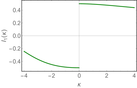
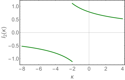
Fig. 11-a		Fig. 11-b

Figure 11: $I_{1}\left(m,\kappa\right)$ ( Fig. 11-a) and $I_{2}\left(m,\kappa\right)$ ( Fig. 11-b) versus $\kappa$ at $m^{2}$=1.

In Fig. 11 we plot the ${\rm Re}I_{1}$ and $I_{2}$ as function of $\kappa$ at $m^{2}=1$. The singularities of $I_{1}$ are easy to see from the explicit expression in Eq. (115): $\kappa=0$ and $\kappa=4(m\,+\,i)$. However, the second singularities for the $\kappa$ dependence of ${\rm Re}I_{1}$ are not obvious. The possible singularities of $I_{2}$ stem from the solution of the equation:

$$4m\kappa+\kappa^{2}-4=0;~{}~{}~{}\kappa_{\pm}\,\,=\,\,2\left(-m\pm\sqrt{m^{2}+1}\right)$$ (118)

However, it is easy to see that, both $\kappa_{+}$ and $\kappa_{-}$ do not correspond to the singularity of $I_{2}$ (see Fig. 11-b).

Plugging Eq. (115) and Eq. (116) into Eq. (114) we obtain

$$\Sigma\left(\kappa\right)\,\,=\,\,\frac{1}{4}{\rm Re}\Bigg{(}\Big{\{}\left(1\,\,+\,\,m_{0}\,i\right)^{2}\,I_{1}\,\,+\,\,\left(1\,\,+\,\,m^{2}_{0}\right)\,I_{2}\Bigg{)}$$ (119)

where $m$ and $m_{0}$ are defined as in Eq. (69) - Eq. (71).

Appendix B The numerical estimates in the variational approach.

As it has been pointed out in Ref.LLS in the integrals in Eq. (82) we have two problems: (i) the very large values of $\kappa$ and $\kappa^{\prime}$ are essential; and (2) the region of $\kappa\,\to\,\kappa^{\prime}$ is very sensitive to the numerical calculation proceedure. Recall that this region in the case of massless BFKL equation leads to a divergency. To heal all these problems we re-write Eq. (69) and Eq. (82) in the following form:

$$E\,\phi\left(\kappa\right)\,\,=\,\,\,-\,T\left(\kappa\right)\,\phi\left(\kappa\right)\,-\,\,\bar{\alpha}_{S}\int d\kappa^{\prime}\,K\left(\kappa,\kappa^{\prime}\right)\,\Bigg{\{}\phi\left(\kappa^{\prime}\right)\,\,-\,\,\frac{G\left(\kappa^{\prime}\right)}{G\left(\kappa\right)}\,\phi\left(\kappa\right)\Bigg{\}}+\,\,m\,\frac{N^{2}+1}{N^{2}_{c}}G\left(\kappa\right)\int d\kappa^{\prime}G\left(\kappa^{\prime}\right)\,\phi\left(\kappa\right)$$ (120)

where $G\left(\kappa\right)$ is given by Eq. (56). One can see that at $\kappa^{\prime}\,\to\,\kappa$ the term in curly brackets vanishes, providing the smooth integration in this dangerous region. For a better control of the interation at large $\kappa$ in Eq. (82) we replace

$$T\left(\kappa\right)\,\,\to\,\,\Bigg{(}T\left(\kappa\right)\,\,-\,\,\ln\kappa\Bigg{)}\,\,+\,\,\ln\kappa$$ (121)

The term in parentheses vanishes at large $\kappa$, leading to a converged integral at large $\kappa$, while the integral for the trial function of Eq. (83) can be taken, leading to the following expression:

$$\int d\kappa\left(\ln\kappa\right)\,\,\phi^{2}_{\rm trial}\left(\kappa\right)\,\,=\,\,-\frac{\sqrt{\pi}4^{-\gamma}\left(\frac{1}{a^{2}}\right)^{\frac{1}{2}-\gamma}\left(a^{2}\right)^{1-2\gamma}\Gamma\left(\gamma+\frac{1}{2}\right)\left((2\gamma-1)\log\left(\frac{1}{a^{2}}\right)-2\right)}{(1-2\gamma)^{2}\Gamma(\gamma)}$$ (122)

All numerical integration were take replacing $\kappa=e^{l}$ and $\kappa^{\prime}=e^{l^{\prime}}$ and $l(l^{\prime})$ runs from $-20$ to $250$.

References

- (1) I. Balitsky, “Operator expansion for high-energy scattering", [arXiv:hep-ph/9509348]; “Factorization and high-energy effective action", Phys. Rev. D60, 014020 (1999) [arXiv:hep-ph/9812311]; Y. V. Kovchegov, “ Small-x structure function of a nucleus including multiple Pomeron exchanges"’ Phys. Rev. D60, 034008 (1999), [arXiv:hep-ph/9901281].
- (2) Yuri V Kovchegov and Eugene Levin, “ Quantum Choromodynamics at High Energies", Cambridge Monographs on Particle Physics, Nuclear Physics and Cosmology, Cambridge University Press, 2012 and references therein
- (3) V. S. Fadin, E. A. Kuraev and L. N. Lipatov, “On the pomeranchuk singularity in asymptotically free theories", Phys. Lett. B60, 50 (1975); E. A. Kuraev, L. N. Lipatov and V. S. Fadin, “The Pomeranchuk Singularity in Nonabelian Gauge Theories" Sov. Phys. JETP 45, 199 (1977), [Zh. Eksp. Teor. Fiz.72,377(1977)];
- (4) I. I. Balitsky and L. N. Lipatov, “The Pomeranchuk Singularity in Quantum Chromodynamics,” Sov. J. Nucl. Phys. 28, 822 (1978), [Yad. Fiz.28,1597(1978)].
- (5) L. N. Lipatov, “The Bare Pomeron in Quantum Chromodynamics,” Sov. Phys. JETP 63, 904 (1986) [Zh. Eksp. Teor. Fiz. 90, 1536 (1986)].
-
(6)
M. Froissart,
Phys. Rev. 123 (1961) 1053;
A. Martin, “Scattering Theory: Unitarity, Analitysity and Crossing." Lecture Notes in Physics, Springer-Verlag, Berlin-Heidelberg-New-York, 1969. - (7) A. Kovner and U. A. Wiedemann, “Nonlinear QCD evolution: Saturation without unitarization,” Phys. Rev. D 66, 051502 (2002) [hep-ph/0112140]; “Perturbative saturation and the soft pomeron,” Phys. Rev. D 66, 034031 (2002) [hep-ph/0204277]; ,̇ “No Froissart bound from gluon saturation,” Phys. Lett. B 551, 311 (2003) [hep-ph/0207335].
- (8) E. Ferreiro, E. Iancu, K. Itakura and L. McLerran, “Froissart bound from gluon saturation,” Nucl. Phys. A 710, 373 (2002) [hep-ph/0206241].
- (9) E. M. Levin and M. G. Ryskin, “High-energy hadron collisions in QCD,” Phys. Rept. 189 (1990) 267.
- (10) E. M. Levin and M. G. Ryskin, “The Shrinkage Of The Diffraction Peak Of The Bare Pomeron In QCD,” Sov. J. Nucl. Phys. 50 (1989) 881 [Z. Phys. C 48 (1990) 231] [Yad. Fiz. 50 (1989) 1417].
- (11) E. Levin and C. I. Tan, “Heterotic pomeron: A Unified treatment of high-energy hadronic collisions in QCD,” In *Santiago de Compostela 1992, Proceedings, Multiparticle dynamics* 568-575 and Fermilab Batavia - FERMILAB-Conf-92-391 (92/09,rec.Jan.93) 9 p. (303600) Brown Univ. Providence - BROWN-HET-889 (92/09,rec.Jan.93); [hep-ph/9302308].
- (12) D. Y. Ivanov, R. Kirschner, E. M. Levin, L. N. Lipatov, L. Szymanowski and M. Wusthoff, “The BFKL pomeron in (2+1)-dimensional QCD,” Phys. Rev. D 58 (1998) 074010 doi:10.1103/PhysRevD.58.074010 [hep-ph/9804443].
- (13) D. Kharzeev and E. Levin, “Scale anomaly and ’soft’ pomeron in QCD,” Nucl. Phys. B 578 (2000) 351 doi:10.1016/S0550-3213(00)00158-9 [hep-ph/9912216].
- (14) D. E. Kharzeev, Y. V. Kovchegov and E. Levin, “QCD instantons and the soft pomeron,” Nucl. Phys. A 690 (2001) 621 doi:10.1016/S0375-9474(01)00352-9 [hep-ph/0007182].
- (15) K. J. Golec-Biernat and A. M. Stasto, “On solutions of the Balitsky-Kovchegov equation with impact parameter,” Nucl. Phys. B 668, 345 (2003) [hep-ph/0306279].
- (16) S. Bondarenko, E. Levin and C. I. Tan, “High energy amplitude as an admixture of ’soft’ and ’hard’ pomerons,” Nucl. Phys. A 732 (2004) 73 doi:10.1016/j.nuclphysa.2003.11.056 [hep-ph/0306231].
- (17) E. Gotsman, M. Kozlov, E. Levin, U. Maor and E. Naftali, “Towards a new global QCD analysis: Solution to the nonlinear equation at arbitrary impact parameter,” Nucl. Phys. A 742, 55 (2004) [hep-ph/0401021].
- (18) Y. Hatta and A. H. Mueller, “Correlation of small-x gluons in impact parameter space,” Nucl. Phys. A 789, 285 (2007) [hep-ph/0702023 [HEP-PH]].
- (19) A. H. Mueller and S. Munier, “Correlations in impact-parameter space in a hierarchical saturation model for QCD at high energy,” Phys. Rev. D 81, 105014 (2010) [arXiv:1002.4575 [hep-ph]].
- (20) J. Berger and A. M. Stasto, “Small x nonlinear evolution with impact parameter and the structure function data,” Phys. Rev. D 84, 094022 (2011) [arXiv:1106.5740 [hep-ph]].
- (21) J. Berger and A. Stasto, “Numerical solution of the nonlinear evolution equation at small x with impact parameter and beyond the LL approximation,” Phys. Rev. D 83, 034015 (2011) [arXiv:1010.0671 [hep-ph]].
- (22) A. Kormilitzin and E. Levin, “Non-linear equation: Energy conservation and impact parameter dependence,” Nucl. Phys. A 849, 98 (2011) [arXiv:1009.1468 [hep-ph]].
- (23) E. Levin and S. Tapia, “BFKL Pomeron: modeling confinement,” JHEP 1307 (2013) 183 [arXiv:1304.8022 [hep-ph]].
- (24) E. Levin, L. Lipatov and M. Siddikov, “BFKL Pomeron with massive gluons,” Phys. Rev. D 89 (2014) 074002 [arXiv:1401.4671 [hep-ph]].
- (25) E. Levin, “Large behaviour in the CGC/saturation approach: BFKL equation with pion loops,” Phys. Rev. D 91 (2015) no.5, 054007 [arXiv:1412.0893 [hep-ph]].
- (26) D. E. Kharzeev and E. M. Levin, “Color Confinement and Screening in the Vacuum of QCD,” Phys. Rev. Lett. 114, no.24, 242001 (2015) doi:10.1103/PhysRevLett.114.242001 [arXiv:1501.04622 [hep-ph]].
- (27) O. V. Kancheli, “On the parton picture of Froissart asymptotic behavior,” arXiv:1609.07657 [hep-ph].
- (28) E. Gotsman and E. Levin, “Large impact parameter behavior in the CGC/saturation approach: A new nonlinear equation,” Phys. Rev. D 101, no.1, 014023 (2020) doi:10.1103/PhysRevD.101.014023 [arXiv:1910.11662 [hep-ph]].
- (29) V. N. Gribov, “Quantization of Nonabelian Gauge Theories,” Nucl. Phys. B 139, 1 (1978)
- (30) V. N. Gribov, “The Theory of quark confinement,” Eur. Phys. J. C 10, 91-105 (1999) doi:10.1007/s100529900052 [arXiv:hep-ph/9902279 [hep-ph]].
- (31) V. N. Gribov, “ORSAY lectures on confinement. 1.,” [arXiv:hep-ph/9403218 [hep-ph]].
- (32) V. N. Gribov, “Orsay lectures on confinement. 2.,” [arXiv:hep-ph/9404332 [hep-ph]].
- (33) V. N. Gribov, “Orsay lectures on confinement. 3.,” [arXiv:hep-ph/9905285 [hep-ph]].
- (34) N. Vandersickel and D. Zwanziger, “The Gribov problem and QCD dynamics,” Phys. Rept. 520, 175 (2012) and references therein.
- (35) Y. L. Dokshitzer and D. E. Kharzeev, “The Gribov conception of quantum chromodynamics,” Ann. Rev. Nucl. Part. Sci. 54, 487 (2004) [hep-ph/0404216].
- (36) D. Dudal, O. Oliveira and P. J. Silva, “High precision statistical Landau gauge lattice gluon propagator computation vs. the Gribov-Zwanziger approach,” Annals Phys. 397, 351-364 (2018) doi:10.1016/j.aop.2018.08.019 [arXiv:1803.02281 [hep-lat]].
- (37) I. Gradstein and I. Ryzhik, Table of Integrals, Series, and Products, Fifth Edition, Academic Press, London, 1994.
- (38) L. V. Gribov, E. M. Levin and M. G. Ryskin, “Semihard Processes in QCD,” Phys. Rept. 100 (1983) 1.
- (39) J. Bartels, E. Levin, “Solutions to the Gribov-Levin-Ryskin equation in the nonperturbative region,” Nucl. Phys. B387 (1992) 617-637;.
- (40) E. Levin and K. Tuchin, “Solution to the evolution equation for high parton density QCD,” Nucl. Phys. B 573 (2000) 833, [hep-ph/9908317].
- (41) E. Iancu, K. Itakura and L. McLerran, “Geometric scaling above the saturation scale,” Nucl. Phys. A 708 (2002) 327 [hep-ph/0203137].
- (42) A. H. Mueller and D. N. Triantafyllopoulos, “The energy dependence of the saturation momentum,” Nucl. Phys. B 640 (2002) 331 [hep-ph/0205167]
- (43) C. Gattringer and C. B. Lang, "Quantum Chromodynamics on the Lattice", Springer-Verlag, Berlin, Heidelberg, 2010; R. Gupta, “Introduction to lattice QCD: Course,” [arXiv:hep-lat/9807028 [hep-lat]]. G. P. Lepage, “Lattice QCD for novices,” [arXiv:hep-lat/0506036 [hep-lat]]; C. Morningstar, “The Monte Carlo method in quantum field theory,” [arXiv:hep-lat/0702020 [hep-lat]].
- (44) D. Dudal, C. P. Felix, M. S. Guimaraes and S. P. Sorella, “Accessing the topological susceptibility via the Gribov horizon,” Phys. Rev. D 96, no.7, 074036 (2017) doi:10.1103/PhysRevD.96.074036 [arXiv:1704.06529 [hep-ph]].
- (45) G. Veneziano, “U(1) Without Instantons,” Nucl. Phys. B 159 (1979) 213.
- (46) E. Witten, “Current Algebra Theorems for the U(1) Goldstone Boson,” Nucl. Phys. B 156, 269 (1979).
- (47) D. Dudal, O. Oliveira and N. Vandersickel, “Indirect lattice evidence for the Refined Gribov-Zwanziger formalism and the gluon condensate in the Landau gauge,” Phys. Rev. D 81, 074505 (2010) doi:10.1103/PhysRevD.81.074505 [arXiv:1002.2374 [hep-lat]].
- (48) A. Cucchieri, D. Dudal, T. Mendes and N. Vandersickel, “Modeling the Gluon Propagator in Landau Gauge: Lattice Estimates of Pole Masses and Dimension-Two Condensates,” Phys. Rev. D 85, 094513 (2012) [arXiv:1111.2327 [hep-lat]].
- (49) D. Dudal, S. P. Sorella, N. Vandersickel and H. Verschelde, “New features of the gluon and ghost propagator in the infrared region from the Gribov-Zwanziger approach,” Phys. Rev. D 77, 071501 (2008) doi:10.1103/PhysRevD.77.071501 [arXiv:0711.4496 [hep-th]].
- (50) D. Dudal, J. A. Gracey, S. P. Sorella, N. Vandersickel and H. Verschelde, “A Refinement of the Gribov-Zwanziger approach in the Landau gauge: Infrared propagators in harmony with the lattice results,” Phys. Rev. D 78, 065047 (2008) doi:10.1103/PhysRevD.78.065047 [arXiv:0806.4348 [hep-th]].
- (51) D. Dudal, S. P. Sorella and N. Vandersickel, “The dynamical origin of the refinement of the Gribov-Zwanziger theory,” Phys. Rev. D 84, 065039 (2011) doi:10.1103/PhysRevD.84.065039 [arXiv:1105.3371 [hep-th]].
- (52) D.Kharzeev and E. Levin, “Fluctuating topology as a solution of UA(1) and confinement problems in QCD",(in preparation).
- (53) A.D. Polyanin, Handbook of linear partial differential equations for engineers and scientists , Chapman Hall/CRC, 2001.