Latent Causal Socioeconomic Health Index

Abstract

This research develops a model-based LAtent Causal Socioeconomic Health (LACSH) index at the national level. Motivated by the need for a holistic national well-being index, we build upon the latent health factor index (LHFI) approach that has been used to assess the unobservable ecological/ecosystem health. LHFI integratively models the relationship between metrics, latent health, and covariates that drive the notion of health. In this paper, the LHFI structure is integrated with spatial modeling and statistical causal modeling. Our efforts are focused on developing the integrated framework to facilitate the understanding of how an observational continuous variable might have causally affected a latent trait that exhibits spatial correlation. A novel visualization technique to evaluate covariate balance is also introduced for the case of a continuous policy (treatment) variable. Our resulting LACSH framework and visualization tool are illustrated through two global case studies on national socioeconomic health (latent trait), each with various metrics and covariates pertaining to different aspects of societal health, and the treatment variable being mandatory maternity leave days and government expenditure on healthcare, respectively. We validate our model by two simulation studies. All approaches are structured in a Bayesian hierarchical framework and results are obtained by Markov chain Monte Carlo techniques.

, and

1 Introduction

The gross domestic product (GDP) has been conventionally used as a measure when benchmarking different countries’ growth and production. However, the commonly used GDP arguably only captures one aspect/perspective—the economic performance of a country—rather than a country’s overall performance and wellbeing. Consequently, many ongoing discussions and much effort have been made to find an alternative ‘wellbeing’ indicator as a holistic measure of a country’s socioeconomic health [Conceição and Bandura (2008)]. Such wellbeing indices are useful for governments and organizations to benchmark a country’s overall performance (other than solely economic) and help policy makers form evidence-based decisions. Despite that, there are issues with existing methods that attempt to quantify this health/wellbeing feature. For instance, multiple sources of subjectivity are combined and arbitrarily turned into a single score, yet without rigorously quantifying the uncertainties around the score [New Economics Foundation (2016); Organisation for Economic Co-operation and Development (2016) (OECD); United Nations Development Programme (2018)], or a country’s wellbeing is taken as a chosen proxy such as the life satisfaction score [Sachs et al. (2018)], which is not a direct measurement of the variable of interest. Health and wellbeing are increasingly being accepted as multidimensional concepts that often involve multiple subjective and objective measures on the macro- and micro-levels [McGillivray and Clarke (2006); Yang (2018)]. We recognize that the concept of wellbeing is inevitably subjective and we focus on reducing the subjectivity on the quantifiable measures through statistical inference of the country’s socioeconomic health as a model parameter.

This paper proposes a LAtent Causal Socioeconomic Health (LACSH) index by developing a hierarchical, latent variable framework to simultaneously model each country’s health as a latent parameter, account for spatial correlation among countries, and evaluate the causal impact of a policy variable on the latent health. This new methodology contributes to the aforementioned effort towards a holistic approach by addressing the subjectivity and uncertainty propagation through a single statistical inferential framework. To assess societal health for countries, the LACSH index builds on the concept of the latent health factor index (LHFI) for modeling the underlying ecosystem health in Chiu et al. (2011) and Chiu et al. (2013) as unobservable and latent.

Note that the approach to measuring latent traits is not unique, as the idea appears in item response theory (IRT) in the psychometrics literature [Rabe-Hesketh and Skrondal (2004)]. Other examples include the quantification of the position of political actors on a political spectrum [Jackman (2001); Martin and Quinn (2002)], constructing measures of nations’ underlying democracy [Treier and Jackman (2008)], and assessing ecological/ecosystem health [Chiu et al. (2011); Chiu et al. (2013)]. Rijpma et al. (2016) model the wellbeing of countries also as a latent variable, similar to the special-case LHFI model that regresses health indicators on $H$ alone. In contrast, the general LHFI model further regresses $H$ on covariates that are chosen due to their perceived explanatory nature to health. In this paper, our holistic framework further incorporates causal modeling and spatial structures into the LHFI framework.

In applying our work, we quantify the latent health of the countries using data collected at the national level. Observable variables (e.g. gross national income (GNI) per capita, life expectancy, mean years of schooling) are treated as either indicators or drivers/covariates of a country’s underlying health condition as opposed to measures of health. We use ‘health’ and ‘wellbeing’ interchangeably to capture the notion of a country’s socioeconomic performance from the social, political, economic and environmental perspectives simultaneously. For the rest of the paper we will continue to refer to this holistic notion as (latent) health when referring to both the model parameter and the concept of wellbeing. As national-level variables tend to be spatially dependent [Ward and Gleditsch (2018)], we incorporate a spatial modeling structure into the LHFI framework to formally model this dependency among the countries. Here, in addition to capturing latent health, we are interested in the counterfactual: what might happen to the country’s health had policy makers altered the value of the policy variable in question?

To this end, we consider propensity score adjustment for reducing confounding bias in observational studies. This technique has been used widely in the literature since the seminal paper by Rosenbaum and Rubin (1983). Subsequently, there have been ample discussions [An (2010); McCandless et al. (2010); Kaplan and Chen (2012); Zigler et al. (2013)] on modeling the uncertainty associated with the inference of the propensity score, as reflected by McCandless et al. (2009) who model the uncertainty under a Bayesian framework to evaluate the impact of statin therapy on mortality of myocardial infarction patients. We extend this idea of using the generalized propensity score framework for continuous treatment to estimate a dose-response function [Hirano and Imbens (2004); Imai and Van Dyk (2004)]. We evaluate the impact of varied doses of a ‘policy treatment’ variable (for illustration purposes, mandatory maternity leave (MML) days and domestic general government health expenditure (GGHE) per capita, respectively) on a country’s health. Including this notion of ‘policy treatment’ in our model allows a model-based assessment of the effect of a policy variable on the (latent) health of a country, in the context of counterfactuals.

To elaborate on the above elements, our paper is laid out as follows. In the next section, we briefly review the methodologies used to construct some of the existing socioeconomic health indices. Section 3 introduces the countries’ data, and Section 4 discusses the methodology and building blocks we employ to construct our latent socioeconomic health for nations. In Section 5, we propose a framework (using the building blocks discussed in Section 4) which is applied to the data, and highlight some of the results from our models; we also discuss a new visualization technique for assessing covariate balance under the generalized propensity score framework. In Section 6, we revisit the data by providing an in-depth discussion of the specifics of the data and model structure we have used. In Section 7, we discuss two simulation studies to validate our model results. Finally, we review the limitations of our work and conclude the paper by discussing some potential future work in Section 8. Appendices A–G in the supplemental document contain further details on computation, posterior distributions, and additional insights.

2 Review on existing indices

2.1 Global and regional indices

There is an increasing awareness that the GDP has been inappropriately used as a broader benchmark measure for overall welfare among countries [Kubiszewski et al. (2014)]. Several methods have been proposed as an alternative measure to the GDP, but existing approaches have used, e.g. the life evaluation score or ‘happiness’ as a proxy measure of a country’s health (or subjective wellbeing) [Sachs et al. (2018); Conceição and Bandura (2008)]. This is also problematic, as a country’s health is a multidimensional concept as aforementioned. We review five such alternative indices in Table 2.1. The background and components contributing to these five and other indices have been discussed by Hashimoto et al. (2018) and Kubiszewski et al. (2014), but here we focus on the statistical methodology being used. Note that 2 out of these 5 indices assume equal weighting of pre-specified variables that contribute to a country’s health. There appears to be little justification apart from convenience, that the concept of health should be represented by equal parts of a wide variety of variables.

Index	Statistical Methodology
United Nations Human Development Index (HDI)58	Arithmetic means of different variables are computed, then a geometric mean of the arithmetic means is computed to form the HDI
World Happiness Report50	Pooled ordinary least squares regression (from econometrics) of the national average response to the survey question of life evaluations on 6 categories of variables hypothesized as underlying determinants of the nation’s ‘happiness score’
Social Progress Index (SPI)55	First, a principal component analysis (PCA) is used to determine the weighting of indicators within each component, and the weights and indicators are multiplied to obtain component scores. Next, component scores are transformed onto a scale of 0-100, an arithmetic mean is computed for each dimension, and another arithmetic mean is computed to obtain the final SPI
Happy Planet Index (HPI)38	The variables ‘experienced wellbeing’ and ‘life expectancy’ are multiplied, then divided by ‘ecological footprint’; scaling constants are used to map the final HPI to range from 0-100
Organisation for Economic Co-operation and Development (OECD) Better Life Index (BLI)41	OECD BLI website user-specified weights are assigned to each topic (e.g. education, income), and up to four indicators which constitute each topic are assigned equal weights to form the final BLI

Table 2.1: Selection of existing indices and methodology used

3 Data

The variables in this work are chosen based on data availability and quality, and in alignment with other existing well-being indices. They can be roughly grouped according to environmental and infrastructure, progressiveness and inclusiveness, education, income and wealth, and demographic variables. We collated our data from the years 2010–2016 from publicly available databases. We consider 15 metrics, $\bm{Y}$, each of 2 treatment variables, $T$, and 4 covariates, $\bm{X}$, shown in Table 3.1.

Most of the metrics and covariates employed in our models are taken from the data section in the United Nations Human Development Report, which is sourced from various organizations and the World Bank database. Specifically, the POLITY variable is sourced from the Polity IV project [Center for Systemic Peace (2016)], and Corruption Perception Index from the Transparency International website [Transparency International (2018)]. Other relevant variables (e.g. literacy rate among adults in the country) were not included in our model due to a substantial amount of missing data.

X, Covariates	T, Treatment variable
Forest area♯	Federally mandated maternity
Access to electricity, rural	leave (MML) days
Mean years of schooling	Domestic general government expenditure
Population, total♭	on health (GGHE) per capita♭
Y, Metrics    Education index		⋆Population density♭
⋆Popn., urban (% of total)	⋆Popn., ages 65 and older♭
⋆Employment to popn. ratio (%)	⋆Unemployment rate (%)♯
⋆Corruption Perception Index♯	Life expectancy∂
Infant mortality rate♯	Internet users (% of popn.)♯
⋆Renewable energy consumption (%)♯	⋆POLITY index∂
Gross National Income (GNI)  per capita (current international $)♭
⋆Prop. of parliamentary seats   held by women (%)♯
Popn. with at least some   secondary education (% ages 25 and older)
⋆Variables included as $Y^{*}$  ♯square-root transformed  ♭log-transformed    ∂cubic-transformed

Table 3.1: List of variables $\bm{X},{T}\text{ and }\bm{Y}$

Literature on Neyman-Rubin’s causal framework advocates the use of pre-treatment variables to answer causal questions. For our case studies, we argue that unlike the policy variables, existing traits on infrastructure and demography are what a country “comes with”. These “inherent” traits are therefore regarded as drivers of socioeconomic health, and as pre-policy-treatment covariates. Specifically, the $Y$’s are indicators of health (e.g. education index) based on measures that we perceive as reflective of a country’s health and regarded as the outcome variables due to various policies. In particular, GNI as opposed to GDP was used as it is perceived as a more inclusive indicator of a country’s wealth [Klugman et al. (2011)]. These indicators, or metrics, have been a priori transformed so that increasing values reflect better health and to reduce skewness; see Section 6.3 for additional details. For our single policy treatment variable $T$, we consider each of the following in two separate models — federally mandated number of maternity leave (MML) days and domestic general government health expenditure (GGHE) per capita. These two variables were chosen based largely on data availability, but also on the fact that their proposed economic and societal benefits [Chapman et al. (2008); Lea (1993)] make them interesting examples to illustrate our methodology. Note that the World Bank data source only has alternate years of maternity leave data, and we had to informally impute the data for some of the OECD countries using data from the OECD website [OECD (2018)]. A discussion of data imputation is found in Section 6.3.

Importantly, it is recognized that the selection of modeled variables is inevitably subjective but still in line with other literature and well-being indices. As such, we focus on the methodology and its interpretation.

4 Methodology

To quantify the latent causal socioeconomic health (LACSH) and its uncertainty in a policy-specific context, we integrate two modern approaches—the latent health factor index (LHFI) [Chiu et al. (2011)] and the generalized propensity score (GPS) methodology and its extensions [Hirano and Imbens (2004), Imai and Van Dyk (2004)]—along with spatial modeling to account for spatial dependence among countries. We are interested in these two methods as the former describes health as latent, i.e. a trait that is not directly measurable, while the latter allows us to examine the effect of policy prescription and estimate the dose-response function for different ‘doses’ of a policy treatment and the corresponding response—a nation’s overall socioeconomic health—as a counterfactual.

4.1 Latent health

As an analogy to a country’s latent health, the underlying health conditions of a person who is deemed healthy cannot be directly compared to those conditions of another person. It is the measurable variables such as height, weight or calorie intake of a person that can be compared. Similarly, for a country, there is no single directly observable quantity that can represent “how well a country is doing”. Thus, the health of a country is a notion that we wish to evaluate comprehensively and holistically. For instance, we may argue that variables like GNI, life expectancy, and infant mortality rate can each coarsely inform us on some aspect of the state in which a country’s health is, but not its overall health. The LHFI framework unifies multiple aspects of health by modeling the underlying condition that we wish to assess as a latent parameter (not directly measurable), but it is dependent on different measurables that are either drivers of health (covariates), or indicators of health (metrics); see Figure 1.

Figure 1: Schematics of a conventional health index and LHFI [adapted from Chiu et al. (2013)]

The LHFI structure employed to model health as a latent variable for our specific context is a type of mixed model [Rabe-Hesketh and Skrondal (2004)], where nation-specific health is a random effect. We formulate our model as a Bayesian hierarchical mixed model, as it is noted in Gelman and Hill (2007) as the most direct approach to handle latent structures.

Martin and Quinn (2002) discuss the unidentifiability issues that are prominent in item response models (a type of generalized linear mixed model) in their work. To address this issue in our framework, we truncate the distribution for one pre-selected country’s health parameter, $H_{anc}$, to anchor our latent score’s scale. A more in-depth discussion of the anchoring approach can be found in Section 6.1.

Note that a country’s metrics are multivariate in nature. Thus, in our hierarchical model, we use a multivariate normal distribution on the first level in the hierarchy, i.e. the metric level (Y-level) (equation (1)). We consider the previous years’ covariates and metrics, averaged over years, as a set of combined covariates that drive the countries’ health in the following year, which, in turn, is reflected by that year’s metrics.

Specifically, we designate the year 2015 as the current year, in which the treatment is administered, and we evaluate its effect on the country’s socioeconomic health and metrics in the following year (2016). Pre-treatment covariates are $\bm{X}^{*}$ and $\bm{Y}^{*}$, where $\bm{X}^{*}$ denotes the averaged covariate values over the years 2010–2014. Similarly, $\bm{Y}^{*}$ denotes the averaged metric values over the years 2010–2014; to avoid collinearity among regressors, we retain only one of the $Y^{*}$’s that show a correlation of 0.8+ with another $Y^{*}$ or an $X^{*}$ (see Table 3.1). In particular, we eliminate the metrics one-by-one until all correlations between $\bm{X}^{*}$ and $\bm{Y^{*}}$ are less than 0.8. Both $\bm{X}^{*}$ and $\bm{Y}^{*}$ are regarded as predictors of latent health in 2016. (The exclusion of 2015 from the definitions of $\bm{X}^{*}$ and $\bm{Y}^{*}$ will be further discussed in Section 4.3.) Therefore, our base LHFI model (excluding spatial elements) with an ‘$H$-anchor’ takes on the form

$$\bm{y_{i}}|\bm{a},H_{i},\Sigma_{Y} \stackrel{{\scriptstyle ind.}}{{\sim}} \text{MVN}(\bm{a}H_{i},\Sigma_{Y})$$ (1)

$$\bm{H}|\bm{\zeta},\bm{W^{*}},\sigma^{2}_{H} \sim \text{TMVN}(\bm{W^{*}}\bm{\zeta},\Sigma_{H})\mathbb{1}\{H_{anc}<0\}$$ (2)

$$\text{where}\ \ \ \Sigma_{H} = \sigma^{2}_{H}{\bm{I}}$$

and where MVN and TMVN denote the multivariate and truncated multivariate normal distributions, respectively. The TMVN is defined as the joint distribution of $N-1$ MVNs (for non-anchor countries) with a truncated normal (for $H_{anc}$). This joint distribution has mean $\bm{W^{*}\zeta}$ and an $N\times N$ diagonal covariance matrix $\Sigma_{H}$, which reflects the naive assumption that countries are independent given the covariates. See Horrace (2005) for full details of the TMVN formulation. Normality is assumed due to the nature of our metric variables (see Section 3).

At the Y-level, we let $\bm{y_{i}}=(y_{i1},\ldots,y_{iP})^{T}$ be a $P\times\text{1}$ vector for the $i$th country’s metrics in the year 2016 for $i=1,\ldots,N$; $\bm{a}=(a_{1},\ldots,a_{P})^{T}$ be the $P\times 1$ vector for the ‘loadings’ of any country’s health on its metrics; and $\Sigma_{Y}$ be the $P\times P$ covariance matrix for the 2016 metrics.

We refer to equation (2) as the health level ($H$-level), where $\bm{H}$ is an $N\times\text{1}$ vector of latent health in 2016 for all $N$ countries including the chosen anchor country; $\bm{W^{*}}=(\bm{1},\bm{T},\bm{X^{*}},\bm{Y^{*}})$ is an $N\times(2+K+Q)$ matrix where $\bm{1}$ is an $N\times 1$ vector of ones; $\bm{T}$ is an $N\times 1$ vector of treatment values in 2015; $\bm{X^{*}}=(\bm{x^{*}_{1}},\ldots,\bm{x^{*}_{K}})$ is an $N\times K$ matrix for $K$ different covariates, $\bm{x^{*}_{k}}$ being an $N\times 1$ vector of the $k$th covariate for $k=1,\ldots,K$, averaged over the years 2010–2014; and $\bm{Y^{*}}=(\bm{y^{*}_{1}},\ldots,\bm{y^{*}_{Q}})$ is an $N\times Q$ matrix where $\bm{y^{*}_{q}}$ is an $N\times 1$ vector of the $q$th metric for $q=1,\ldots,Q$, also averaged over the years 2010–2014 (and $Q\textless P$); $\bm{\zeta}=(\zeta_{0},\zeta_{1},\ldots,\zeta_{K+Q+1})^{T}$ is a $(2+K+Q)\times 1$ vector including the intercept and slope coefficients corresponding to the treatment variable, the five-year averaged pre-treatment covariates and the five-year averaged pre-treatment metrics; $\sigma^{2}_{H}$ is the common variance for $H_{i}$ for all $i$ including $H_{anc}$; $\bm{I}$ is an $N\times N$ identity matrix; finally, $H_{anc}$ for the chosen anchor country is restricted in $(-\infty,0)$ (see Section 6.1 for justification).

Note that the raw metrics are on vastly different scales, so we standardize each metric to have mean zero and unit variance. As such, the overall intercept of the model appears at the $H$-level rather than the $Y$-level. A discussion of data transformations is found in Section 6.3.

4.2 Spatial modeling

Ward and Gleditsch (2018) and Darmofal (2015) note that there are very few examples of point-level data in the social sciences. In addition, spatial correlations among countries are often not accounted for, even though macro-level variables of countries are expected to be spatially correlated, as countries that are close together in regions (e.g. Europe, North America and Central Asia) tend to be more similar in terms of a cultural, economic, social or political context. This suggests that the latent health of countries may also be spatially dependent. In order to assess the need for spatial modeling in our framework, we fit the base LHFI model, treating the policy variable as a typical covariate, in this case MML, using equations (1) - (2) and examined its residuals. The residuals are defined as

$$\bm{\widehat{\epsilon_{H}}}^{*}=\bm{H}-\bm{X\zeta}$$

where $\bm{\widehat{\epsilon_{H}}}^{*}$ is the posterior median of the residuals after subtraction on the right-hand-side based on the Markov chain Monte Carlo (MCMC) samples.

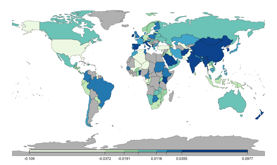
Figure 2: Residuals $\bm{\widehat{\epsilon_{H}}}^{*}$ on the world map. Gray regions are not represented in our dataset

Figure 2 presents the residuals from the base LHFI model fit on the world map. It is apparent that countries that are geographically close together in regions such as North America, Western Europe, Central and South East Asia have residuals that are either similarly under- or over-estimated by our base model. Similarly, the model that replaces MML with GGHE (map not shown) also shows the need to address spatial dependency. To accommodate this, in the next section we incorporate spatial dependency among residuals on the health level, and modify equation (2) to account for this spatial dependence in its residuals.

4.3 Causal inference

In addition to quantifying our latent socioeconomic health and its uncertainty, we seek to integrate causal modeling into our framework to provide insight into the effect of a ‘policy treatment’ variable on the health of a country.

Two schools of thought dominate the causal inference literature — namely, “Pearl’s causal diagram” [Pearl (2009)] and “Rubin’s causal model” [Imbens and Rubin (2015)]. Both attempt to establish causal effects from observational studies, which was previously considered impossible because such studies are not randomized controlled trials [Imbens and Rubin (2015); Hernán and Robins (2020)]. Among causal inference methods for non-experimental data, propensity score (PS) analysis (stratification, matching and covariate adjustment) in the so-called Rubin’s approach has been widely used to address selection bias. In our current work under the Rubin framework, instead of dichotomizing the continuous treatment variables, we consider the generalized propensity score (GPS), which were developed similarly by Hirano and Imbens (2004) and Imai and Van Dyk (2004), to estimate the dose-response function. The GPS approach is an extension to the propensity score method for binary treatments and multi-valued treatments [Rosenbaum and Rubin (1983); Imbens (2000)]. It allows us to fully utilize the raw information while reducing the ambiguity due to an arbitrary quantile used to categorize treatments. We follow the specifications as laid out by Hirano and Imbens (2004) in our work.

In the case of binary treatments, there has since been research that considers the uncertainty in the propensity scores [McCandless et al. (2009); An (2010)], although incorporating the outcome variable at the stage where the inference of the PS is conducted may be contentious [Kaplan and Chen (2012); Zigler et al. (2013); Zigler (2016)]. For this reason, our GPS framework extends the work by Zigler et al. (2013) for binary treatment, whereby we use the Bayesian posterior predictive distribution of the GPS to separate the design stage and analysis stage in order to ‘cut the feedback’ (i.e. to ensure that the inference of the GPS does not depend on the outcome variable) [McCandless et al. (2010); Zigler et al. (2013); Zigler and Dominici (2014)]. Cutting the feedback is further explored by Stephens et al. (2023); like various discussants of this work, we take the viewpoint that cutting the feedback is fully consistent with the Bayesian paradigm. See Appendix A for implementation details.

Irrespective of a categorical or continuous treatment variable, there are three main assumptions in Rubin’s approach of causal modeling, namely, (i) the stable unit treatment value assumption (SUTVA), which stipulates no interference between units [Rubin (2005)]; (ii) strongly ignorable treatment assignment, which stipulates no unmeasured confounders [Rosenbaum and Rubin (1983)]; and (iii) consistency, where the potential outcome of the treatment must correspond to the observed response when the treatment variable is set to the observed ‘exposure’ level [Cole and Frangakis (2009)]. For the GPS method, Hirano and Imbens (2004) generalize (ii) to the weak unconfoundedness assumption, which only requires conditional independence for each value of the treatment ($H(t)\perp T\ |\ X,\text{ for all }t\in T$) as opposed to joint independence for all potential outcomes.

However, incorporating causal modeling in a spatial setting potentially violates the no interference assumption (SUTVA) as discussed at length in Keele and Titiunik (2015) and Noreen (2018). In investigating the effect of convenience voting and voter turnout, Keele and Titiunik (2015) are concerned about interference and spillover effects – the units (individuals) may be influenced due to proximity of geographical regions (or influenced at the workplace or by their social network, etc.).

In our paper, the causal question of interest is the effect of a national policy variable on a country’s health, with the unit of interest being at the national-level rather than at the individual-level. We consider two policy variables in our work. For the mandatory maternity leave (MML) variable, two obvious scenarios of interference and spillover in our case may be a) individuals immigrating or emigrating and in their newly adopted country, either influencing policy makers or affecting the health of the country (e.g. a Canadian mother whose wellbeing benefited from the Canadian federal maternity leave policy emigrates to the United States, which does not have federal maternity leave, thus possibly improving the health of the United States); b) policy makers being influenced by their international social networks.

The second policy variable of interest is domestic general government health expenditure (GGHE) per capita in a country. Note that ‘health’ in this variable refers to the individual-level’s public healthcare funding rather than the countries’ overall socioeconomic health $H$. We argue that the potential scenarios of interference and spillover are similar to a) and b) mentioned above.

Here, we can assume minimal effects of individuals’ international migration on MML, GGHE, or socioeconomic health at the national level. Additionally, we can assume that federal policy making regarding maternity leave and public healthcare expenditure is a collective domestic effort and generally conducted with minimal foreign interference. Finally, as discussed by Schutte and Donnay (2014), when there is only minor overlap in the units, a consistent treatment effect can still be valid. These arguments suggest that SUTVA is reasonable in our case.

Moreover, we utilize structural variables, namely, the country’s existing infrastructure and the average of previous years’ metrics as covariates in our framework. This is to align with the approach by Rubin (2005) of conditioning on the pre-treatment variables. We can assume that the current year’s policy treatment is affected by metrics and covariates from previous years. We assume that, given these observable pre-treatment covariates through the GPS, a country’s choice of MML days and GGHE is random, and that there are no unmeasured important confounders. Hence, we proceed with the GPS framework while assuming that the required assumptions (i), (ii), and (iii) hold.

Our GPS formulation is based on work by Hirano and Imbens (2004). Similar to the PS approach for the binary case, in which the PS is the probability of receiving treatment given the covariates, the GPS is defined as the conditional probability density of the continuous treatment given the covariates. The relevant properties and methodology are discussed at length in Hirano and Imbens (2004) and Kluve et al. (2012). The ‘outcome variable’ in our work is the country’s latent health. A schematic representation is presented in the left panel of Figure 3 and we represent the full inference and causal DAG in the right panel.

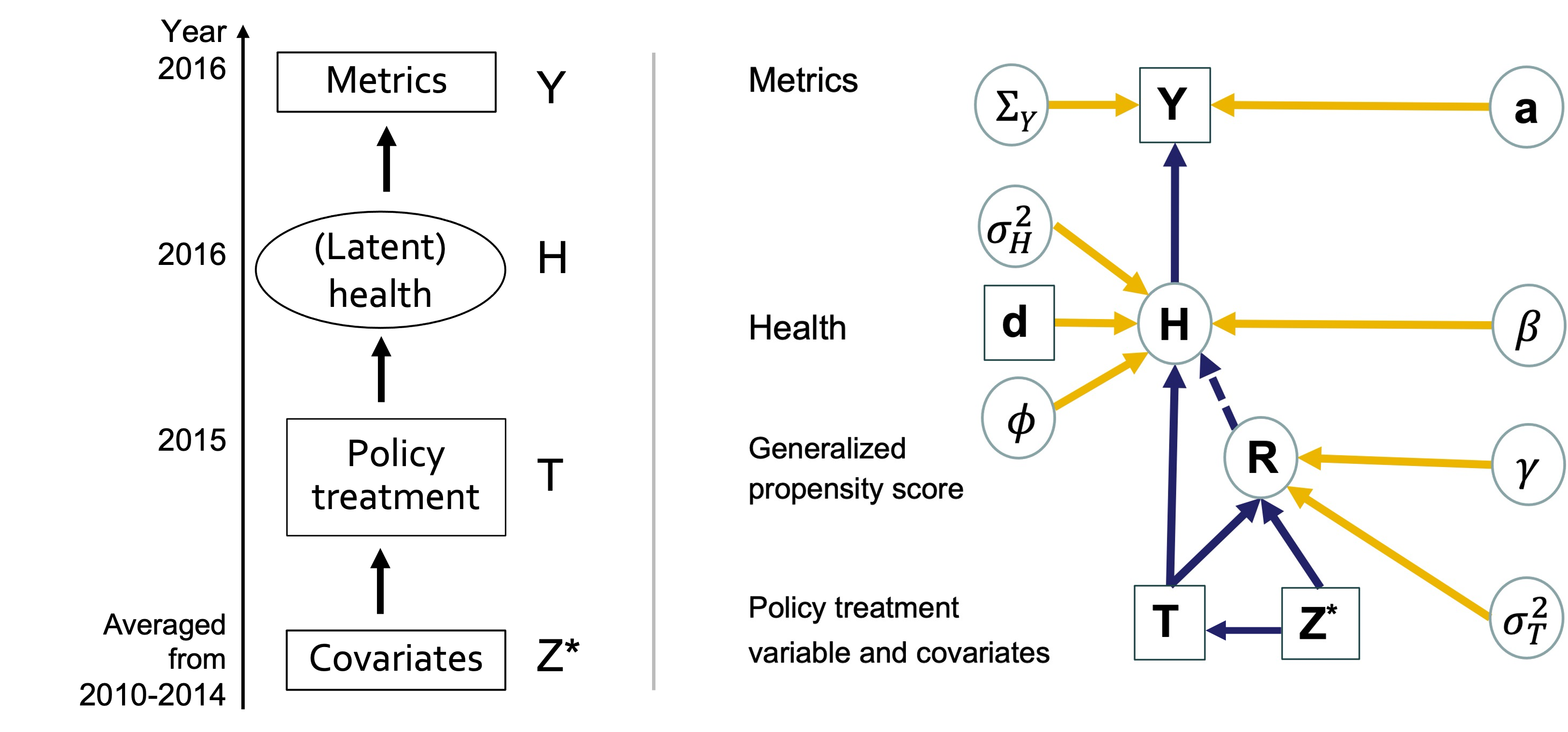
Figure 3: Left panel: Extension of the LHFI framework with causal modeling. Right panel: Causal directed acyclic graph (DAG) of our full LACSH model (dark purple arrows only) and the model’s inference graph (arrows in either color), where the dashed arrow indicates ‘cutting the feedback’.

As such, we propose the LHFI methodology that includes causal and spatial modeling as the LAtent Causal Socioeconomic Health (LACSH) index. To incorporate causal modeling into our spatial LHFI model, we introduce the policy treatment variable $T$ and its generalized propensity score $R=r(T,\bm{\gamma},\bm{Z^{*}},\sigma^{2}_{T})$ to our health-level through its mean (however, note the special MCMC implementation in Appendix A regarding “cutting the feedback” in the MCMC):

$$\bm{y_{i}}|\bm{a},H_{i},\Sigma_{Y} \stackrel{{\scriptstyle ind.}}{{\sim}} \text{MVN}(\bm{a}H_{i},\Sigma_{Y})$$ (3)

$$\bm{H}|\bm{\beta},\bm{T},\bm{R},\Sigma_{H} \sim \text{TMVN}(\bm{\mu},\Sigma_{H})\mathbb{1}\{H_{anc}<0\}$$ (4)

$$\vspace{2em}T_{i}|\bm{Z^{*}}_{i},\bm{\gamma},\sigma^{2}_{T} \stackrel{{\scriptstyle ind.}}{{\sim}} \text{N}(\bm{Z^{*}}_{i}\bm{\gamma},\sigma^{2}_{T})$$ (5)

$$\text{where}\hskip 30.00005pt[\bm{\mu}]_{i} = \beta_{0}+\beta_{1}T_{i}+\beta_{2}T_{i}^{2}+\beta_{3}R_{i}+\beta_{4}R_{i}^{2}+\beta_{5}T_{i}R_{i}$$ (6)

$$R_{i}=r(T_{i},\bm{\gamma},\bm{Z^{*}_{i}},\sigma^{2}_{T}) = \frac{1}{\sqrt{2\pi}\sigma_{T}}\text{exp}\left(-\frac{1}{2\sigma_{T}^{2}}(T_{i}-\bm{Z^{*}}_{i}\bm{\gamma})^{2}\right)$$ (7)

$$\Sigma_{H} = \sigma_{H}^{2}\mathbf{\Omega}(d,\phi)$$ (8)

$$\mathbf{\Omega}(d,\phi) = \begin{bmatrix}1&\rho_{12}&\cdots&\rho_{1n}\\ \rho_{21}&1&\ddots&\vdots\\ \vdots&\ddots&\ddots&\rho_{n-1,n}\\ \rho_{n1}&\cdots&\rho_{n,n-1}&1\\ \end{bmatrix}$$ (9)

$$\rho_{nm} = exp(-d_{nm}/\phi)=\rho_{mn}$$ (10)

where $\Sigma_{H}$ denotes the $N\times N$ spatial covariance matrix for health; $\rho_{nm}$ is the correlation parameter between countries $n$ and $m$, which is a function of both $d_{nm}$ (the great circle distance (GCD) between capital cities of two countries and $\phi$ (the ‘range’ or inverse rate of decay parameter).

In equation (6), $T_{i}$ is the policy treatment variable of interest in 2015, $R_{i}=r(\cdot)$ is the GPS, and $\bm{\beta}=(\beta_{0},\beta_{1},\ldots,\beta_{5})^{T}$ are the associated regression coefficients. The inclusion of quadratic and interaction terms of the GPS and treatment variable are described in Section 5.3. In equation (7), $\bm{Z^{*}}_{i}$ is the $i$th row vector of the $N\times(K+Q)$ matrix $\bm{Z^{*}}=(\mathbf{1},\bm{X^{*}},\bm{Y^{*}})$, whose columns are the $N\times 1$ vector of ones, and the covariates and metrics averaged over 2010–2014 (as described in Section 4.1); the corresponding $(1+K+Q)\times 1$ regression coefficient vector is $\bm{\gamma}=(\gamma_{0},\gamma_{1},\ldots,\gamma_{K+Q})^{T}$.

The covariance function we employ in equations (8) - (10) is a special case of the Matérn class of spatial covariance functions, for modeling the dependence between spatial observations [Gelfand et al. (2010)]. For instance, a large value of $\rho$ suggests that countries that are relatively far from one another are still moderately correlated [Hoeting et al. (2006)]. Note that while we consider GCDs, geographical distance measures on a global scale have always been a contentious issue [Ward and Gleditsch (2018)]. We discuss some possible extensions to the spatial component in our framework in Section 6.2.

5 Latent Health for the World

We present results from our LACSH model (spatial causal LHFI in Section 4.3), separately fitted to the countries’ data using MML days and GGHE as the treatment variable. The posterior credible intervals of rankings of countries are provided in Appendix B, and the resulting LACSH rankings using the two different treatment variables are compared to each other and also to the HDI and SPI rankings on ladder plots in Appendix C.

For Bayesian inference, an adaptive MCMC algorithm [Roberts and Rosenthal (2009)] was used to automatically tune all parameters on the $H$-level, and as well as $H_{anc}$ in the MCMC due to non-conjugacy and to improve convergence and mixing. All other parameters were sampled using Gibbs sampling. Specific sampling specifications are documented in Appendix A. For model results, we utilized roughly 100,000 post-burn-in MCMC samples from the posterior distribution. Standard diagnostics (e.g. trace plots in Table 5.1 and effective sample sizes in Appendix D) suggested that each parameter of the MCMC chain had reached its steady state.

5.1 Priors

We specify conjugate diffuse priors for most parameters. For each regression coefficient $a_{j}$, $\beta_{k}$, and $\gamma_{l}$, the variance parameter log($\sigma^{2}_{H}$), and the spatial correlation parameter log$(\phi)$, we specify a normal prior distribution with mean 0 and variance 100. The covariance matrix $\Sigma_{Y}$ is given an inverse-Wishart prior with $P+2$ degrees of freedom, and an identity scale matrix. The diffuse prior for $\sigma^{2}_{T}$ is inverse gamma with shape = 1 and scale = 0.01.

5.2 Ranking of countries according to latent health, $H$

I. MML days

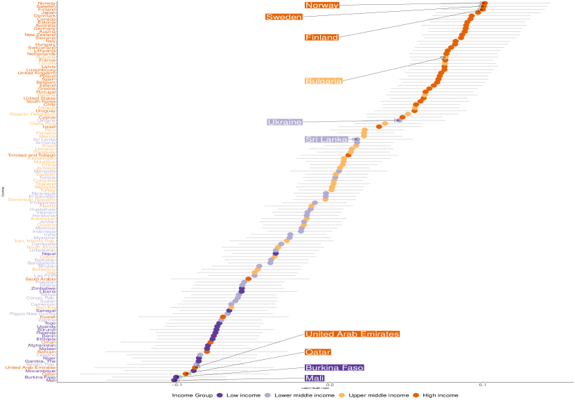
Figure 4: Latent health for 120 countries in 2016 color-coded by income group, with MML as treatment

a Figure 4 shows the country ranking based on the posterior medians of the $H$’s (colored dots) along with their corresponding 90% credible intervals (gray bands). The figure highlights some countries that are ranked highest, lowest, or differently than its United Nations’ (UN) designated income group. Exceptions include United Arab Emirates (UAE) and Qatar, which belong to UN’s high income group, but are ranked low by our LACSH index when using MML as policy treatment, and also by the Social Progress Index [Stern et al. (2020)]. Indeed, MML may be seen as a strong social progress indicator. Formal quantification of the uncertainty for our health parameter suggests that countries are not polarized into developed/developing countries or rich/poor countries; the lack of polarization aligns with the findings in Rosling (2019).

Nevertheless, our color-coding according to the designated income groups shows that the countries are generally ranked according to their income group. This suggests that the health of a country is highly correlated with the income group of the country. However, as will be discussed below, income is not necessarily the most important index to examine when considering the health of a country.

The posterior median and corresponding credible interval for the highest-ranked, lowest-ranked, and anchor country are shown in Table 5.1.

II. GGHE

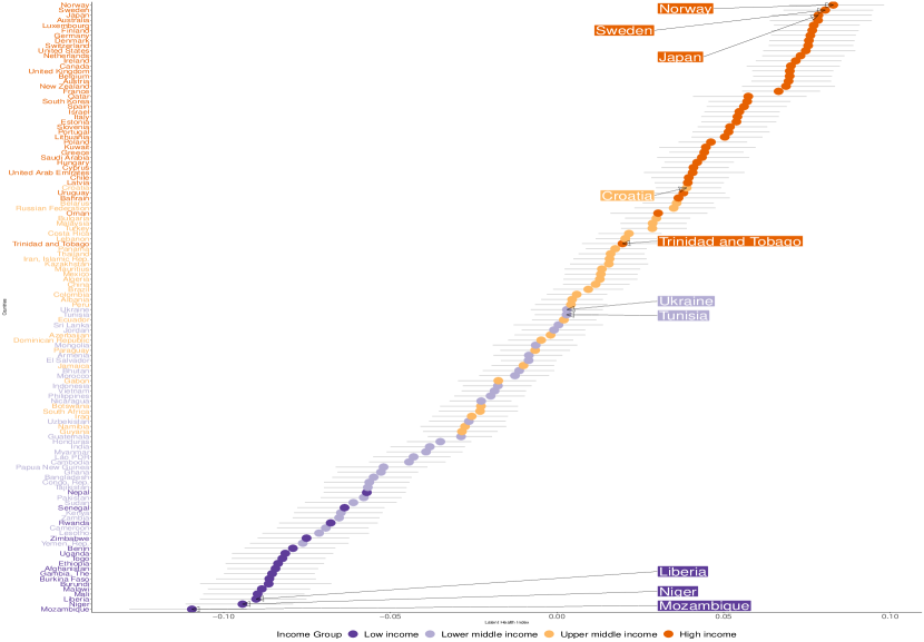
Figure 5: Latent health for 120 countries in 2016 color-coded by income group, with GGHE as treatment

The countries’ health ranking using GGHE as the treatment variable is shown in Figure 5. Compared to using MML as treatment, this ranking shows tighter credible intervals (narrower gray bands) and follows the UN’s designated income groups more closely. This may be due to the high correlation between the GGHE treatment variable and many metrics and covariates (e.g. ‘mean years of schooling’, ‘GNI per capita’).

Some exceptions are Ukraine and Sri Lanka, which are classified as lower-middle income countries by the United Nations, but are ranked among the high and upper-middle income countries in our rankings in both models fitted using MML and GGHE as treatment. These results suggest that a country’s health is not solely reflected by its income or wealth.

5.3 Numerical results and implications

Posterior summaries for selected parameters are shown in Table 5.1. The other model parameters are tabulated in Appendix B.

Nations’ latent health, $H$

Table 5.1 left panel shows the highest and lowest ranked $H_{i}$ from our LACSH model using MML as treatment, corresponding to Norway ($i=$ 84) and Mali ($i=$ 73). Based on the 90% credible intervals, Figure 4 suggests that there are no stark differences from country to country. Nevertheless, we can consider potential groupings by examining the posterior probability of a positive difference in health between countries. For the top-ranked countries, the posterior probability for Norway to be in better health than Sweden is negligible at 0.53, for Sweden to be better than Finland is 0.51, whereas for Finland to be better health than Japan is 0.57, suggesting the four countries may be grouped together. Similar calculations of posterior probabilities can also be easily obtained for other countries.

Some of the posterior summaries for our LACSH model using GGHE as treatment are tabulated in the right panel of Table 5.1. Norway ($i=$ 84) is again ranked at the top, similar to using MML as treatment, followed by Sweden ($i=$ 104), Japan ($i=$ 57) and Australia ($i=$ 5). However, similar calculations of posterior probability of difference as above again suggest these countries may be grouped together. Mali and Mozambique remain in the bottom five of our ranking for results from both treatment variables.

Health loadings, $\bm{a}$

Insights into the associated strength and direction of relationship between metrics and health are available from the inference about the health loadings, $a_{j}$. These results demonstrate that our model-based approach does not require a priori input on which metrics reflect ‘good’ health, or which metrics are important to a country’s latent health.

Table 5.1 left panel shows the results based on the marginal posterior medians using MML as treatment variable, for the three metrics which receive the highest positive impact from health, and one example of a negative loading, which will be discussed via Figure 6.

In decreasing order of effect size, the corresponding positively affected metrics are: ‘population, ages 65 and older (% of total)” ($j=$ 9), ‘education index’ ($j=$ 1) and ‘infant mortality rate (per 1,000 live births)’ (reversed-scale) ($j=$ 6). This suggests that, among the 15 metrics, population health-themed and education variables receive the highest three loadings from the country’s latent health.

The right panel of Table 5.1 shows some of the results for GGHE as treatment. The posterior probability is 0.66 for health to have a bigger effect on ‘GNI per capita’ ($j=$ 3) than ‘infant mortality rate (per 1,000 live births)’ (reversed-scale) ($j=$ 6), and is 0.55 for ‘infant mortality rate’ than ‘internet users(% of population)’ ($j=$ 4), suggesting that the latent health of countries has similarly weighted effects on the three metrics receiving the highest positive impact. The different results between MML and GGHE suggest that which metrics are most affected by health depends on the treatment variable in the model. Other relevant discussions for GGHE as treatment are given in Appendix E.

Parameter	MC	5%	Median	95%
$H_{84\phantom{,}\text{(Norway)}}$		0.07	0.10	0.14
$H_{73\phantom{,}\text{(Mali)}}$		-0.15	-0.10	-0.07
$H_{anc}$		-0.12	-0.07	-0.04
$a_{9}$		10.97	14.80	19.02
$a_{1}$		9.07	12.74	16.68
$a_{6}$		8.90	12.73	16.78
$a_{2}$		-7.35	-4.17	-1.38
$\beta_{1}$		-0.02	-0.01	0.00
$\sigma_{H}^{2}$		0.002	0.005	0.011
$\phi$		3.37	5.37	8.82
$\gamma_{1}$		-0.10	0.04	0.17

Parameter	MC	5%	Median	95%
$H_{84\phantom{,}\text{(Norway)}}$		0.07	0.08	0.10
$H_{76\phantom{,}\text{(Mozambique)}}$		-0.13	-0.11	-0.09
$H_{anc}$		-0.11	-0.09	-0.07
$a_{3}$		15.43	17.81	20.23
$a_{6}$		15.10	17.41	19.83
$a_{4}$		14.97	17.30	19.73
$a_{15}$		-13.64	-10.86	-8.26
$\beta_{1}$		0.04	0.04	0.05
$\sigma_{H}^{2}$		0.002	0.003	0.004
$\phi$		27.10	29.64	33.16
$\gamma_{1}$		-0.04	0.11	0.26

Table 5.1: Posterior summaries for selected LACSH model parameters, with MML and GGHE as treatment, respectively

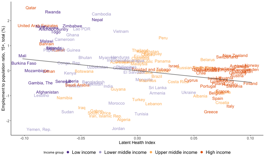
Figure 6: Plot of employment-to-population ratio vs. LACSH model posterior median of latent health, with MML as treatment, and with a least squares regression fit for visualization

Figure 6 shows a weak negative relationship between the metric ‘employment to population ratio’ and a country’s latent health (90% credible interval for $a_{2}$ is $(-7.35,-1.38)$). As we can see from the figure, countries with a high proportion of employment-to-population ratio are generally in the low-income group, and the ratio decreases with increasing income. This perhaps goes against the naive belief that a high employment ratio reflects a country’s ‘good’ health. There are several possible explanations for this result. One, wages are typically low in low-income countries, resulting in a higher proportion of the population having to work in order to secure a decent living wage. Two, lower-income countries relatively lack effective social safety nets and social protection systems for its population, resulting in a higher proportion of the population working for a longer period of time until (a possibly later) retirement age. Some exceptions are Qatar and UAE, which are high-income countries but also have high employment ratio due to a large proportion of its population being expatriate workers [Parcero and Ryan (2017)].

Given the other metrics in the model, for MML as treatment, three metrics namely, ‘population density’, ‘unemployment rate’ (reversed-scale), and ‘renewable energy consumption’ were found to have no substantial statistical relationship with a country’s latent health. For GGHE as treatment, the metric ‘proportion of seats held by women in national parliament’ also shows no statistical relationship with a country’s latent health as opposed to ‘renewable energy consumption’. In fact, the model suggests there is a negative relationship between ‘renewable energy consumption’ and a country’s latent health. We provide further discussions in Appendix E.

Average dose-response function

To examine the dose-response function which relates the inherent impact of varied levels of a policy treatment variable on the country’s health, we utilize the GPS formulation as proposed by Hirano and Imbens (2004). The GPS approach allows us to evaluate a country’s health outcome that corresponds to each specified value of the continuous treatment (i.e. MML days or GGHE). Note that the conditional expectation of the outcome as a function of the treatment $T$ and the GPS $R$ is $\beta(t,r)=E[H|T=t,R=r]$ for each specified treatment ‘dose’ $t\in T$.

We can obtain an estimate of the entire dose-response function through estimating the average potential outcome at a given $t$. In particular, $\mu(t)=E[H_{i}(t)]$ is calculated similar to equation (6) but substituting specific values of $t$ for $T$ in equations (6) and (7). The entire dose-response function is then $\mu(t)=E[\beta\{t,r(t,\bm{Z_{i}}^{*})\}]$, which is estimated by $\hat{\mu}(t)=(1/N)\sum_{i}\beta\{t,r(t,\bm{Z_{i}}^{*})\}$. As $\hat{\mu}(t)$ depends on the parameters $\bm{\beta}$ and $\bm{\gamma}$, we examine the posterior median of $\hat{\mu}(t)$ at a given $t$ (red curves in Figures 7 and 8).

Hirano and Imbens (2004) assert that the conditional expectation of the outcome as a function of the treatment level $T$ and the GPS $R$ ($\beta(t,r)$) does not have a causal interpretation, but that $\mu(t)$ which corresponds to the dose-response function for treatment level $t$, when compared to another value of $t^{\prime}$, does have a causal interpretation.

Many authors in the GPS literature use quadratic and interaction terms of the GPS and treatment variable in its conditional expectation of the outcome. We examine the need for the quadratic terms, by comparing both models with and without the terms in equation (6) using the Watanabe-Akaike information criterion (WAIC), also known as the widely applicable information criterion, which is useful for models with a hierarchical structure and in which the number of parameters grows with the sample size [Watanabe (2010); Gelman et al. (2014); Statisticat and LLC. (2020)]. We find that quadratic terms are needed for GGHE but not MML (WAIC values 3032.35 (quadratic) and 3026.84 for MML, and 2950.37 (quadratic) and 3742.99 for GGHE). To discuss the comparison between MML and GGHE, we keep the quadratic terms.

Figures 7 and 8 show the posterior average dose-response function using thinned posterior samples (for visualization purposes) from our LACSH model (eq. (4) - (7)).

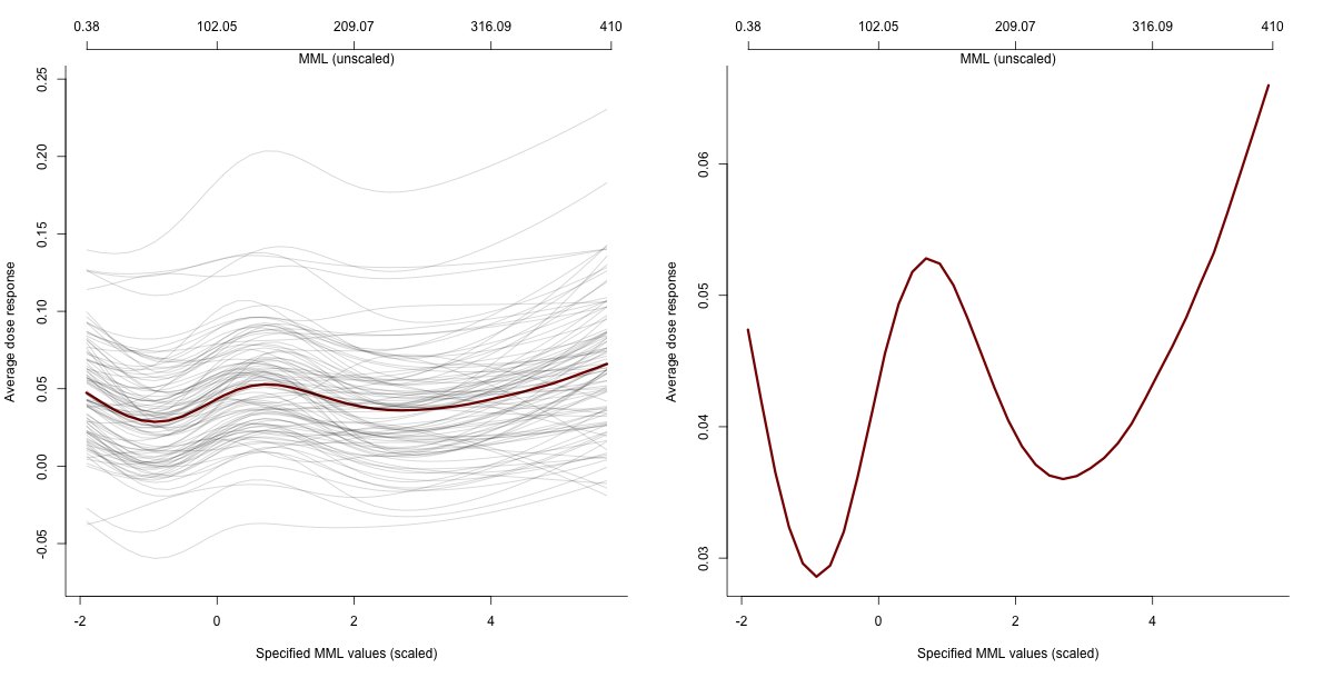
Figure 7: The LACSH model posterior median dose-response function (red), with MML as treatment, and with 100 thinned MCMC samples (gray) for visualization of uncertainty

The left panel in Figure 7 shows gray curves as the posterior dose-response based on a thinned MCMC sample; the red curve indicates the posterior median based on approximately 100,000 MCMC scans. The curves show a very weak increase (with a slight blip) in the average dose-response as the number of MML days increases. The right panel, the curve of posterior median zoomed-in vertically, shows an increasing dose-response when MML days range over 53-145 and 236-410. Upon further inspection, the double ‘dip’ may be due to the lack of data around certain ranges of MML days with clusters of countries having similar MML values.

Figure 8: The LACSH model posterior median dose-response function (red), with GGHE as treatment, and with 100 thinned MCMC samples (gray) for visualization of uncertainty

The average dose-response function shown in Figure 8 suggests that increasing the level of health expenditure (GGHE) monotonically leads to an increased level of the country’s health. The figure also presents strong evidence of a causal phenomenon, in that all posterior samples in the figure are monotone.

Assessing covariate balance under the generalized propensity scores framework

In Rubin’s approach of causal inference, the balance between treatment and control groups with respect to the pre-treatment covariates is a crucial assumption [Imbens and Rubin (2015)]. We introduce a novel technique to visually assess covariate balance in the GPS framework. Generally, testing for covariate balance with a continuous treatment variable is not straightforward, and we consider the approaches by both Hirano and Imbens (2004) and Imai and Van Dyk (2004) (as noted in Kluve et al. (2012)) to test for:

$$\bm{Z_{i}^{*}}\perp\mathbb{1}\{T_{i}=t\}\ |\ r(t,\bm{Z_{i}^{*}})$$

where the GPS $r(\cdot)$ is evaluated at different specified values of $t$ for the continuous treatment variable. Specifically, we divide the sorted data of $\{T_{1},\ldots,T_{N}\}$ into moving blocks of 20 observations, overlapping 10 observations between neighboring blocks. (This results in 11 blocks for $N=$120 observations.) The GPS is then evaluated at the median of each block.

As the GPS is a dimension reduction tool to control for what is usually a large number of covariates, we investigate covariate balance collectively instead of what is done in the literature, being on each individual covariate. Specifically, we represent the covariates by its first principal component $f(\cdot)$ when evaluating

$$f(\bm{Z_{i}^{*}})\perp\mathbb{1}\{T_{i}=t\}\ |\ r(t,\bm{Z_{i}^{*}})$$ (11)

where $t$ is the block median,

$\mathbb{1}\{T_{i}=t\}=\left\{\begin{array}[]{ll}&1\ \text{if country }i\text{ is in the current block of 20 countries}\\ &0\ \text{otherwise}\end{array}\right.$

and $r(\cdot)$ is computed as $r(t;u_{i},v)=\frac{1}{v\sqrt{2\pi}}\text{exp}(-\frac{(t-u_{i})^{2}}{2v^{2}})$ where $u_{i}$ and $v$ are based on a standalone frequentist linear multiple regression of the $T$ data on the $\bm{Z^{*}}$ data, such that $u_{i}$ is the fitted value for the $i$th country, and $v$ is the fitted residual standard error.

To evaluate if equation (11) holds, first, for each block of 20 countries, we run a frequentist logistic regression of $\mathbb{1}\{T_{i}=t\}$ on $f$ and $r(\cdot)$ and record the $p$-value of the slope for $f$. A $p$-value exceeding, say, 0.1, suggests that the covariates, given the GPS, are not significantly related to the treatment variable at and around that median value. Because the main objective of the GPS methodology is to remove any potential biases introduced by the covariates, we consider the set of 11 $p$-values collectively, whereby covariate balance is deemed adequate if most of the 11 $p$-values satisfy 0.9 $>$ 1-$p$. In the case of MML, left panel of Figure 9 shows there are 5 out of 11 blocks that are above the 0.9 threshold, but if we used 0.95 then 8 out of 11 blocks show adequate covariate balance. The right panel of Figure 9 shows the same blocks that contribute to the overall imbalance whether we use 0.9 or 0.95 as the threshold.

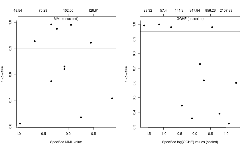
Figure 9: Plot of p-values (reversed-scale) for assessing covariate balance, with MML as treatment (left panel), and with GGHE as treatment (right panel).

In addition to ‘blocking on the (generalized propensity) score’ to assess covariate balance [Imai and Van Dyk (2004)], our novel approach described here also allows us to identify the ranges of treatment values that may be the sources of any overall imbalance. The observations that fall under those ranges may be further investigated for improving overall covariate imbalance, if necessary. In the case of MML (left panel of Figure 9), there are no consistent patterns of covariate imbalance. In contrast, in the case of GGHE (right panel of Figure 9), the lower range of GGHE values (approximately 0-90) consistently show covariate imbalance. To further investigate this, we removed countries in those ranges and re-ran our model on the subsample of countries, which removed the consistent pattern of imbalance. More details are in Appendix F.

Inverse decay parameter $\phi$ and spatial correlation function $\rho(d,\phi)$

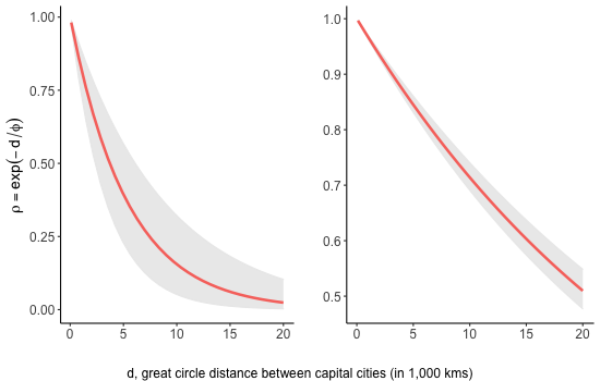
Figure 10: Spatial correlation based on the posterior of $\rho=exp(-\frac{d}{\phi})$ as a function of $d$, under the LACSH model with MML as treatment (left panel), and with GGHE as treatment (right panel).

Figure 10 shows the posterior median of the spatial correlation function $\rho$ evaluated at a given $d$ between capital cities, under the LACSH model with MML and GGHE as treatment, respectively. Both panels show decreasing spatial correlation between the countries as distance increases. The model with MML has a sharper decrease but with more uncertainty (wider credible band) compared to GGHE. For the two countries whose capitals are furthest apart (Spain and New Zealand), our models yield noticeable spatial correlation (90% credible intervals of $(0.02,0.10)$ and $(0.51,0.55)$) with MML and GGHE as treatment, respectively. These results suggest that the LACSH models would be inadequate if spatial dependence were not accounted for.

6 Some technical details

6.1 Identifiability

Recall that at the metric level (Y-level), $a_{j}$ is the population-level loading of a country’s health on its $j$th metric. However, similar to the discussions by Chiu and Westveld (2011) and Martin and Quinn (2002), modeling health $H_{i}$ as a random effect leads to an unidentifiable $\bm{a}$ vector unless constraints are imposed.

The constraint we have utilized in our models is a TMVN distribution on the $H$-level so that the health of an anchor country is negative (or positive, if desired). To decide on the anchor country, we conducted a pilot run of the base LHFI model in Section 4.1 but without any anchor, then selected a low-income group country (Burundi, in this case) on the extreme end of the $H$-scale as the anchor in all subsequent formal models.

As the ranking of a country is relative to the others’, the constraint restricts the anchor country’s health in the negative space and imposes this fixed scale on all other countries. This constraint solves the parameter identifiability issue along with aiding the interpretation of $H_{i}$, as it encodes in the model the fact that a higher value of $H_{i}$ should be interpreted as a higher level of health, not lower.

We have explored alternative constraints, including a ‘soft anchor’ (fixing mean and variance for $H_{anc}$), a ‘hard anchor’ (fixing $H_{anc}$ to a constant), and transposing the $H$-scale manually post-MCMC sampling (so the scale of $H$ aligns with increasing value of $H$ corresponding to increasing levels of health). While our ‘truncated anchor’ leads to additional computational burden, we believe this constraint to be the most desirable as it results in the most flexible approach.

6.2 Spatial distances

Section 5.3 shows that there is considerable spatial correlation among countries, so that not accounting for it would result in model inadequacy. To limit the amount of additional model complexity in our LACSH model, spatial correlation between countries was modeled through the simplest Matérn covariance function in the form of an exponential decay over great circle distances between capital cities of countries. Due to the earth’s spherical nature, Euclidean distances may be inappropriate on a global scale [Banerjee (2005)], and therefore to define neighbors, Gleditsch and Ward (2001) also use a minimum distance between countries based on country borders of up to a certain distance. When we extend the LACSH model to more complex forms in order to formally incorporate dependencies jointly across time (2010–2016) and space (see Section 8), we may explore this minimum distance measure, as well as alternative covariance functions.

6.3 Data transformation and missing values

Higher unemployment rate is generally regarded as bad for societal health [Wulfgramm (2014); Helliwell and Huang (2014)]. For this reason, the metric for the ‘infant mortality rate’ had been linearly transformed prior to modeling so that higher values reflect better societal health. The same transformation was also applied to the metric for ‘unemployment rate’. In practice, the modeler needs not to carry out this transformation, because the fitted model can be used to distinguish the strength and direction of the relationship between latent health and metrics, as reflected by the signs of the health loadings $a_{j}$ on metrics. For instance, the results from both of our treatment variables suggest that higher values of latent health are associated with higher values of the (reversed-scale) infant mortality rate metric (equivalent to low infant mortality rate in the country before the data transformation). In other words, it is inferred that countries with better latent health have low infant mortality rate, conditioned on the set of metrics and covariates that are included in our model. Other visualizations and summaries of the posterior distribution for the negative health effect, $a_{j}$, are included in Appendix E in the supplementary material.

Note that the selection of variables to be included as metrics and covariates in our model was largely based on the availability of data. Initial model fits included more covariates; however, due to collinearity, past-year metrics with a correlation higher than the arbitrary threshold of 0.8 with other covariates/metrics were removed sequentially from modeling. While this paper focuses on the development of methodology, when applying the methodology in practice, the covariates and metrics could be specified by the modeler more according to their domain knowledge and less to data availability. In either case, the issue of missing data may require special attention.

In this paper, we considered two continuous ‘policy treatment’ variables separately in our models. In particular, for MML days, the data obtained from the World Bank only include MML data every other year. Therefore, data for the years 2010, 2012, and 2014 are considered missing. For those years, only countries with the same values for the years before and after the missing year entered our model. To further reduce data missingness in each year, OECD data were used for some OECD countries when MML was missing from the World Bank data, although we note that the two organizations have slightly different definitions of maternity leave. For example, according to the World Bank, Sweden has zero MML days based on its definition. However, the OECD and other sources suggest that this may not be an accurate representation of their maternity policy. (As such, future iterations of our work will consider non-World Bank definitions.)

In our work, given the right-skewed nature of GGHE, we log-transformed the values before standardization. MML days also appeared skewed, but the data appeared in clusters, thus showing large unobserved ranges, and various transformations did not improve the data distribution. For this reason, we had kept the variable untransformed other than standardizing it to have mean zero and unit variance. In future extensions of the current work, we may consider other approaches such as rank likelihood estimation when using treatment variables that are distributed in clusters. All transformations including those in Table 3.1 are intended to adhere to our normality assumptions.

Finally, even if data exist in published records, it is recognized that such data collected on the country-level by various world organizations may have been derived from different and unpublished imputation techniques. Of course, the quality of the data would depend on the actual imputation techniques employed. Moreover, one may not rule out the possibility that data or official statistics reported by certain countries may have been fabricated. Although these disadvantages could reduce the accountability of our modeling results, overcoming such data-related challenges is beyond the scope of our paper.

7 Simulation studies

To validate our models, we ran two simulations. The first is a cross validation study to recover missing metric $Y$ values. The second study assesses the ability to recover true parameter values. Detailed results of the simulations are shown in Appendix G.

In the cross validation study, we use the original data in the paper where our metric $\bm{Y}$ is an $N\times Q$ matrix, where $N=120$ and $Q=15$. We randomly select 100 values (about 5%) from the original $N\times Q$ values of $y_{ij}$ and discard them. In the inference, the 100 missing values are treated as model parameters and estimated alongside all the other parameters. We repeat this process 10 times, each time resulting in a different set of missing values. For each set of 100, we record the number of withheld $y_{ij}$’s that are captured by the 95% posterior predictive intervals. We find that among the 10 sets, the lowest capture rate for missing $y_{ij}$’s is 90% (90/100) and the highest is 98% (98/100).

In the second simulation study, we generate fictitious data based on a version of our model. We fix the parameter values on the $T$-, $H$- and $Y$-levels and generate new $T$’s, $H$’s and $Y$’s, each time the dimension for $\bm{Y}$ is $N^{*}\times Q^{*}$, where $N^{*}=10$ and $Q^{*}=3$. We set $\sigma_{H}=\sigma_{T}=1$; $\phi=5$; $\gamma=0.5$; $\bm{a}=(0.14,0.12,0.08)$; $\Sigma_{Y}$ is fixed with a once-randomly generated $3\times 3$ Wishart-distributed matrix with degrees of freedom 3. Three sets of $\bm{\beta}$ values were used — $\{(2,3,3),(2,-3,-3),(2,-3,\frac{(-\beta_{0}+\beta_{1}\bar{T})}{\bar{R}})\}$, where $\bar{T}$ and $\bar{R}$ are medians of $T$ and $R(\cdot)$ values from the generated $T$’s. We fit our LACSH model and compute the 95% credible interval for each parameter. We repeat the entire process 50 times for each of the three sets of $\bm{\beta}$ values. We find that the capture rate ranges from 70% (35/50) to 100% (50/50).

8 Discussion and future work

In this paper, we developed a LACSH model-based approach that models spatially correlated latent traits alongside the evaluation of policy effects through the integration of LHFI with a causal modeling framework. Through rigorous handling of quantitative treatment variables and the uncertainty quantification that directly results from the integrated LACSH modeling, we have demonstrated that our novel unified framework and visual assessment of covariate balance can be valuable to evidence-based social science with causal implications. Our methodology has been validated through simulations discussed in the previous section.

As mentioned in Section 4.3, to facilitate formal causal inference, our LACSH approach incorporates the Bayesian extension of the generalized propensity score in the spatial LHFI framework. In addition, we intend to consider the alternative framework of Pearl’s causal diagram approach, which could reveal if, by controlling for certain variables, we have unintentionally opened some ‘backdoor paths’ in the causal diagram which would result in spurious correlation [Pearl (2009)]. In the literature, backdoor paths are any non-causal paths between the treatment and outcome variables in the causal diagram. As such, Pearl’s approach might prompt us to explore controlling for a different set of variables and potentially lead to a different scientific conclusion.

In addition to a spatial correlation function to account for dependencies using great circle distances between countries, one might also explore the use of clustering to account for potential cultural or political ideology of countries, but that is beyond the scope of our current paper. Note that other types of distance measures and neighborhood structures may also be explored, although island countries that do not share borders (e.g. Australia, New Zealand, and Sri Lanka) should be handled with care. Regarding temporal data, currently, metrics from 2016 are hierarchically regressed on the treatment from 2015 and the GPS, which depends on temporally averaged covariates and metrics from 2010–2014. A substantively more complex model would be required to formally model temporal correlation in any of $Y,H,T\text{ and }X,$ as an extension to this paper. This would result in a spatio-temporal hierarchical causal model. We anticipate that careful consideration of separability (or otherwise) between space and time will be required.

Also of interest may be formal inference that allows us to identify which metrics are crucial in reflecting the health of a country. To do so, we would consider modeling the health loadings as proportions that sum to 1, resulting in a type of variable/model selection framework. The implication of such a parameterization is the reduction in any modeler-induced selection bias due to choosing variables that are a priori perceived as being important in reflecting a country’s health.

Lastly, existing causal frameworks that jointly handle multiple treatment variables are not readily adaptable to our LACSH framework. The extended rank likelihood approach by Kuh (2022) may be further explored for this purpose.

[Acknowledgements] This research has been supported by an IBISWorld philanthropic donation by the late Phil Ruthven to the Australian National University in the form of research funds awarded to GS Chiu. We thank the handling editor and reviewers for their valuable input. We also thank Beatrix Jones, Bruce Chapman, Carolyn Huston, Corwin Zigler, Paul Gustafson, Peter Mueller, Tim Higgins, and the attendees of Bayes on the Beach 2017 and Joint Statistical Meeting 2018 for stimulating discussions and constructive comments on the topic. The authors acknowledge William & Mary Research Computing (https://www.wm.edu/it/rc) for providing computational resources and technical support that have contributed to the results reported within this paper.

Appendix A MCMC algorithm

All model inference is done through MCMC sampling. All parameters are updated via Gibbs sampling except for some of the parameters on the $H$-level, because equations (4.2) and (4.4) are a combination of $N-1$ multivariate normals and a truncated normal:

1. Sample $H_{i|-i}$ from its N($M,V$) full conditional distribution where:

   $$V=\left(\bm{a}^{T}\Sigma_{Y}^{-1}\bm{a}+D^{-1}\right)$$

   $$M=V^{-1}\left(\bm{a}^{T}\Sigma_{Y}\bm{y_{i}}+D^{-1}m_{i}\right)$$

   $$D=\Sigma_{H[i,i]}-\Sigma_{H[i,-i]}^{T}\Sigma_{H[-i,-i]}^{-1}\Sigma_{H[-i,i]}$$

   $$m_{i}=\mu_{i}+\Sigma_{H[i,-i]}^{T}\Sigma_{H[-i,-i]}^{-1}(H_{[-i]}-\mu_{-i})$$

   $$\bm{\mu}=\mathbf{(1,T,T^{2},R,R^{2},TR)}\bm{\beta}$$

   $$\text{for }i=1,\ldots,N;i\neq\text{anc}$$

2. Sample $\bm{a}=(a_{1},\ldots,a_{P})^{T}$ from its MVN($\bm{M}$, $\bm{V}$) full conditional distribution where:

   $${\bm{V}}=\left(\sum_{i=1}^{N}H_{i}^{2}\Sigma_{Y}^{-1}+100\bm{I_{P}}\right)$$

   $$\bm{M}=\bm{V}^{-1}\left(\Sigma_{Y}^{-1}\mathbf{Y}^{T}\bm{H}\right)$$

   where $\bm{I_{P}}$ is a $P\times P$ identity matrix and $P=15$.

3. Sample $\Sigma_{Y}$ from its Inv-Wishart($\nu_{n}$, $\bm{S_{n}}$) full conditional distribution where:

   $$\nu_{n}=\nu_{0}+N$$

   $$\bm{S_{n}}=(\mathbf{Y}-\bm{H}\bm{a}^{T})^{T}(\mathbf{Y}-\bm{H}\bm{a}^{T})+\bm{I_{P}}$$

   where $\nu_{0}=P+2$, $N=120$ and $\bm{I_{P}}$ is as described above.

4. Sample $\sigma^{2}_{T}$ from its Inverse-Gamma($\alpha_{n}$, $\beta_{n}$) full conditional distribution where:

   $$\alpha_{n}=N/2+1$$

   $$\beta_{n}=\sum_{i=1}^{N}D_{i}^{2}/2+0.01$$

   $$D_{i}=T_{i}-\bm{Z_{i}}^{*}\bm{\gamma}$$

5. Sample $\bm{\gamma}=(\gamma_{1},\ldots,\gamma_{9})^{T}$ from MVN($\bm{M}$, $\bm{V}$) where:

   $${\bm{V}}=\left(\sigma^{-2}_{T}\bm{Z^{*T}}\bm{Z^{*}}+100\bm{I_{(1+K+Q)}}\right)$$

   $${\bm{M}}=\sigma^{-2}_{T}{\bm{V}}^{-1}\bm{Z^{*T}}\bm{T}$$

   where $\bm{I_{(1+K+Q)}}$ is a $(1+K+Q)\times(1+K+Q)$ identity matrix and $(1+K+Q)=10$. This MVN distribution is proportional to $\prod^{n}_{i=1}P(T_{i}|\gamma,\sigma^{2}_{T})P(\gamma)$ which is not a full conditional for $\bm{\gamma}$, in order to ‘cut the feedback’ [McCandless et al. (2010); Zigler et al. (2013)]. This approximate conditional for $\bm{\gamma}$ is then used as the posterior predictive on the $H$-level. Note that this approximation ignores the ($H$-level) contribution from the (country’s health) outcome, thus cutting the feedback.
   

6. Sample the $H$-level parameters ($\bm{\beta}^{\star},\text{log}(\sigma^{2\star}_{H}),\text{log}(\phi^{\star}),H_{i=anc}^{\star}$) as a vector from the proposal distribution $Q_{s}(\bm{u},\cdot)$ as set out below. In particular, the Metropolis algorithm is performed with a scan-specific proposal distribution; for $s\leq 200$, take $Q_{s}(\bm{u},\cdot)=\text{MVN}(\bm{u},(0.1)^{2}\bm{I}_{d}/d)$, whereas for $s>200$, take $Q_{s}(\bm{u},\cdot)=(0.9)\text{MVN}(\bm{u},v^{2}\Sigma_{s}/d)+(0.1)\text{MVN}(\bm{u},(0.1)^{2}\bm{I}_{d}/d)$ where $\bm{u}=$ our parameter vector in the previous MCMC iteration; $d=$ dimension of our target distribution; $v=2.38$ for MML and $v=5$ for GGHE. The different values for $v$ were adapted from Roberts and Rosenthal (2009) to improve slow mixing.
   

   We define the ratio of densities as ${\displaystyle\kappa=\frac{p(\bm{\beta}^{\star},\text{log}(\sigma^{2\star}_{H}),\text{log}(\phi^{\star}),H_{i=anc}^{\star}|\bm{R},\bm{T},H_{i\neq anc})}{p(\bm{\beta},\text{log}(\sigma^{2}_{H}),\text{log}(\phi),H_{i=anc}|\bm{R},\bm{T},H_{i\neq anc})}}$ and accept $(\bm{\beta}^{\star},\text{log}(\sigma^{2\star}_{H}),\text{log}(\phi^{\star}),H_{i=anc}^{\star})\text{ jointly with probability }\kappa\land 1.$

Appendix B Results for LACSH models

B.1 Posterior summaries for LACSH model, MML as treatment variable

Table B.1: Posterior median of parameters using MML as treatment variable, and associated 90% credible intervals

$a_{j}$	5%	50%	95%
$a_{1}$	9.07	12.74	16.68
$a_{2}$	-7.35	-4.17	-1.38
$a_{3}$	6.39	10.20	14.15
$a_{4}$	7.31	11.02	14.94
$a_{5}$	8.53	12.35	16.39
$a_{6}$	8.90	12.73	16.78
$a_{7}$	-3.17	-0.11	2.93
$a_{8}$	8.06	11.58	15.42
$a_{9}$	10.97	14.80	19.02
$a_{10}$	4.66	8.14	11.90
$a_{11}$	2.02	4.83	8.14
$a_{12}$	-4.47	-1.44	1.46
$a_{13}$	7.40	10.88	15.00
$a_{14}$	6.84	9.83	13.34
$a_{15}$	-7.66	-3.59	0.53
$\sigma_{H}^{2}$	0.00	0.01	0.01
$\phi$	3.37	5.37	8.82
$\Sigma_{Y\{2,12\}}$	0.68	0.53	0.68
$\Sigma_{Y\{3,15\}}$	-0.47	-0.69	-0.47
$\Sigma_{Y\{10,15\}}$	-0.40	-0.61	-0.40
$\Sigma_{Y\{3,4\}}$	0.40	0.22	0.40
$\Sigma_{Y\{4,15\}}$	-0.40	-0.62	-0.40

$\beta_{k}$	5%	50%	95%	p($\beta>0\ |$ data)
$\beta_{0}$	-0.01	0.04	0.10	0.89
$\beta_{1}$	-0.02	-0.01	0.00	0.09
$\beta_{2}$	-0.00	0.00	0.00	0.94
$\beta_{3}$	-0.20	-0.01	0.18	0.47
$\beta_{4}$	-0.24	0.07	0.41	0.64
$\beta_{5}$	0.03	0.08	0.12	0.99
$\gamma_{(1+K+Q)}$	5%	50%	95%	p($\gamma>0\ |$ data)
$\gamma_{0}$	-0.11	0.00	0.11	0.50
$\gamma_{1}$	-0.10	0.04	0.17	0.68
$\gamma_{2}$	-0.21	-0.08	0.05	0.15
$\gamma_{3}$	-0.11	0.02	0.14	0.58
$\gamma_{4}$	-0.07	0.07	0.20	0.79
$\gamma_{5}$	-0.09	0.03	0.14	0.65
$\gamma_{6}$	-0.02	0.12	0.26	0.92
$\gamma_{7}$	-0.15	-0.03	0.08	0.33
$\gamma_{8}$	-0.14	-0.01	0.12	0.44
$\gamma_{9}$	-0.11	0.02	0.15	0.59
$\gamma_{10}$	-0.13	-0.01	0.11	0.43
$\gamma_{11}$	-0.19	-0.07	0.06	0.19
$\gamma_{12}$	-0.13	0.00	0.13	0.51
$\gamma_{13}$	-0.21	-0.08	0.05	0.16

$j$	Metrics, Y
1	Education index
2	Employment to popn. ratio, 15+, total (%)
3	GNI per capita (2011 PPP$)
4	Internet users (% of popn.)
5	Life expectancy at birth, total (years)
6	Mortality rate, infant (per 1,000 live births)
7	Population density
8	Popn. with at least some secondary education (% ages 25 and older)
9	Popn., ages 65 and older (% of total)
10	Popn., urban (% of total)
11	Proportion of seats held by women in national parliaments (%)
12	Unemployment, total (% of total labor force)
13	POLITY index
14	Corruption Perception Index
15	Renewable energy consumption (% of total final energy consumption)
$K+Q$	Previous years’ covariates, $Z^{*}=(X^{*},Y^{*})$
1	Access to electricity, rural (% of rural population)
2	Employment to population ratio, 15+, total (%)
3	Forest area (% of land area)
4	Mean years of schooling (years)
5	Population density
6	Population, ages 65 and older (% of total)
7	Population, total
8	Population, urban (% of total)
9	Renewable energy consumption (% of total final energy consumption)
10	Proportion of seats held by women in national parliaments (%)
11	Unemployment, total (% of total labor force)
12	POLITY index
13	CPI

Table B.2: Posterior median of latent health of countries in LACSH using MML as treatment variable, and associated 90% credible intervals

$H_{i}$	5%	50%	95%
$H_{1}$	-0.11	-0.08	-0.05
$H_{2}$	0.03	0.06	0.08
$H_{3}$	-0.15	-0.09	-0.04
$H_{4}$	-0.01	0.02	0.04
$H_{5}$	0.06	0.09	0.13
$H_{6}$	0.06	0.09	0.12
$H_{7}$	-0.04	-0.02	0.01
$H_{8}$	-0.12	-0.07	-0.04
$H_{9}$	0.05	0.07	0.10
$H_{10}$	-0.11	-0.08	-0.05
$H_{11}$	-0.14	-0.10	-0.07
$H_{12}$	-0.07	-0.04	-0.01
$H_{13}$	0.05	0.08	0.11
$H_{14}$	-0.15	-0.08	-0.03
$H_{15}$	0.04	0.06	0.10
$H_{16}$	-0.00	0.02	0.04
$H_{17}$	-0.08	-0.05	-0.02
$H_{18}$	-0.08	-0.05	-0.02
$H_{19}$	0.06	0.09	0.13
$H_{20}$	0.06	0.08	0.11
$H_{21}$	0.03	0.06	0.09
$H_{22}$	-0.01	0.01	0.03
$H_{23}$	-0.10	-0.06	-0.04
$H_{24}$	-0.10	-0.06	-0.03
$H_{25}$	-0.02	0.00	0.02
$H_{26}$	0.02	0.04	0.06
$H_{27}$	0.02	0.05	0.07
$H_{28}$	0.06	0.09	0.13
$H_{29}$	0.07	0.09	0.13
$H_{30}$	-0.02	-0.00	0.02

	5%	50%	95%
$H_{31}$	-0.04	-0.01	0.02
$H_{32}$	-0.02	0.00	0.02
$H_{33}$	0.05	0.07	0.10
$H_{34}$	0.07	0.09	0.13
$H_{35}$	-0.11	-0.08	-0.05
$H_{36}$	0.07	0.10	0.14
$H_{37}$	0.05	0.08	0.11
$H_{38}$	-0.07	-0.04	-0.01
$H_{39}$	0.05	0.07	0.11
$H_{40}$	-0.09	-0.06	-0.03
$H_{41}$	-0.12	-0.09	-0.06
$H_{42}$	0.04	0.07	0.10
$H_{43}$	-0.03	-0.01	0.01
$H_{44}$	-0.04	-0.02	0.01
$H_{45}$	-0.04	-0.02	0.01
$H_{46}$	0.05	0.08	0.11
$H_{47}$	0.06	0.08	0.12
$H_{48}$	-0.04	-0.02	0.00
$H_{49}$	-0.05	-0.03	-0.00
$H_{50}$	0.04	0.07	0.10
$H_{51}$	-0.07	-0.03	0.00
$H_{52}$	-0.09	-0.05	-0.02
$H_{53}$	0.01	0.03	0.06
$H_{54}$	0.06	0.08	0.12
$H_{55}$	-0.01	0.01	0.03
$H_{56}$	-0.05	-0.02	0.01
$H_{57}$	0.07	0.10	0.14
$H_{58}$	-0.02	0.01	0.04
$H_{59}$	-0.09	-0.06	-0.04
$H_{60}$	-0.06	-0.03	-0.01

	5%	50%	95%
$H_{61}$	0.03	0.06	0.09
$H_{62}$	-0.13	-0.07	-0.03
$H_{63}$	-0.08	-0.05	-0.02
$H_{64}$	-0.01	0.01	0.04
$H_{65}$	-0.10	-0.06	-0.02
$H_{66}$	-0.01	0.02	0.05
$H_{67}$	-0.13	-0.08	-0.05
$H_{68}$	0.05	0.08	0.11
$H_{69}$	0.05	0.07	0.11
$H_{70}$	0.05	0.07	0.11
$H_{71}$	-0.04	-0.02	0.01
$H_{72}$	-0.00	0.02	0.05
$H_{73}$	-0.15	-0.10	-0.07
$H_{74}$	-0.05	-0.03	0.00
$H_{75}$	-0.03	0.01	0.04
$H_{76}$	-0.13	-0.09	-0.05
$H_{77}$	-0.02	0.01	0.03
$H_{78}$	-0.12	-0.08	-0.05
$H_{79}$	-0.02	0.00	0.02
$H_{80}$	-0.10	-0.06	-0.04
$H_{81}$	-0.13	-0.09	-0.05
$H_{82}$	-0.02	-0.00	0.02
$H_{83}$	0.05	0.08	0.11
$H_{84}$	0.07	0.10	0.14
$H_{85}$	-0.06	-0.04	-0.01
$H_{86}$	0.06	0.09	0.12
$H_{87}$	-0.14	-0.08	-0.03
$H_{88}$	-0.09	-0.06	-0.03
$H_{89}$	0.00	0.02	0.04
$H_{90}$	-0.00	0.02	0.05

	5%	50%	95%
$H_{91}$	-0.03	-0.01	0.01
$H_{92}$	-0.10	-0.07	-0.04
$H_{93}$	0.05	0.07	0.10
$H_{94}$	0.04	0.06	0.09
$H_{95}$	-0.01	0.01	0.04
$H_{96}$	-0.16	-0.09	-0.04
$H_{97}$	0.02	0.05	0.08
$H_{98}$	-0.11	-0.07	-0.04
$H_{99}$	-0.10	-0.05	-0.01
$H_{100}$	-0.10	-0.06	-0.03
$H_{101}$	-0.10	-0.07	-0.04
$H_{102}$	-0.02	-0.00	0.02
$H_{103}$	0.06	0.09	0.12
$H_{104}$	0.07	0.10	0.14
$H_{105}$	-0.11	-0.07	-0.04
$H_{106}$	-0.02	0.00	0.03
$H_{107}$	-0.07	-0.04	-0.01
$H_{108}$	-0.02	0.01	0.04
$H_{109}$	-0.02	0.00	0.02
$H_{110}$	-0.02	0.00	0.02
$H_{111}$	-0.11	-0.07	-0.05
$H_{112}$	0.02	0.05	0.08
$H_{113}$	0.03	0.06	0.09
$H_{114}$	0.04	0.06	0.09
$H_{115}$	-0.07	-0.04	-0.01
$H_{116}$	-0.04	-0.01	0.01
$H_{117}$	-0.13	-0.09	-0.06
$H_{118}$	-0.07	-0.03	-0.00
$H_{119}$	-0.11	-0.07	-0.04
$H_{120}$	-0.09	-0.06	-0.03

Table B.3: Countries used in LACSH model

$i$	Country
1	Afghanistan
2	Albania
3	United Arab Emirates
4	Armenia
5	Australia
6	Austria
7	Azerbaijan
8	Burundi (Anchor country)
9	Belgium
10	Benin
11	Burkina Faso
12	Bangladesh
13	Bulgaria
14	Bahrain
15	Belarus
16	Brazil
17	Bhutan
18	Botswana
19	Canada
20	Switzerland
21	Chile
22	China
23	Cameroon
24	Congo, Rep.
25	Colombia
26	Costa Rica
27	Cyprus
28	Germany
29	Denmark
30	Dominican Republic

$i$	Country
31	Algeria
32	Ecuador
33	Spain
34	Estonia
35	Ethiopia
36	Finland
37	France
38	Gabon
39	United Kingdom
40	Ghana
41	Gambia, The
42	Greece
43	Guatemala
44	Guyana
45	Honduras
46	Croatia
47	Hungary
48	Indonesia
49	India
50	Ireland
51	Iran, Islamic Rep.
52	Iraq
53	Israel
54	Italy
55	Jamaica
56	Jordan
57	Japan
58	Kazakhstan
59	Kenya
60	Cambodia

$i$	Country
61	South Korea
62	Kuwait
63	Lao PDR
64	Lebanon
65	Liberia
66	Sri Lanka
67	Lesotho
68	Lithuania
69	Luxembourg
70	Latvia
71	Morocco
72	Mexico
73	Mali
74	Myanmar
75	Mongolia
76	Mozambique
77	Mauritius
78	Malawi
79	Malaysia
80	Namibia
81	Niger
82	Nicaragua
83	Netherlands
84	Norway
85	Nepal
86	New Zealand
87	Oman
88	Pakistan
89	Panama
90	Peru

$i$	Country
91	Philippines
92	Papua New Guinea
93	Poland
94	Portugal
95	Paraguay
96	Qatar
97	Russian Federation
98	Rwanda
99	Saudi Arabia
100	Sudan
101	Senegal
102	El Salvador
103	Slovenia
104	Sweden
105	Togo
106	Thailand
107	Tajikistan
108	Trinidad and Tobago
109	Tunisia
110	Turkey
111	Uganda
112	Ukraine
113	Uruguay
114	United States
115	Uzbekistan
116	Vietnam
117	Yemen, Rep.
118	South Africa
119	Zambia
120	Zimbabwe

Table B.4: Posterior median ranks of countries in LACSH using MML as the treatment variable, and associated 90% credible intervals

Country	5%	50%	95%
Finland	1	4	14
Norway	1	4	16
Sweden	1	4	15
Japan	1	5	20
Canada	1	8	24
Denmark	2	8	20
Estonia	2	9	22
Australia	1	10	28
Austria	3	10	22
Germany	2	10	22
New Zealand	3	11	27
Slovenia	3	12	25
Italy	2	14	29
Hungary	4	15	28
Switzerland	6	17	30
Lithuania	7	18	31
Netherlands	6	19	32
Bulgaria	5	20	32
France	8	20	31
Croatia	7	20	32
Luxembourg	7	20	32
Latvia	7	20	33
United Kingdom	9	22	33
Spain	7	23	35
Poland	10	23	33
Belgium	11	24	34
Ireland	12	26	36
Greece	11	28	37
Belarus	12	29	38
Portugal	14	29	38
United States	17	30	38
South Korea	15	31	39
Chile	19	32	40
Albania	20	33	39
Uruguay	15	33	42
Russian Federation	18	35	43
Cyprus	27	36	43
Ukraine	24	37	44
Costa Rica	33	40	48
Israel	33	41	53

Country	5%	50%	95%
Peru	37	44	58
Mexico	37	45	57
Panama	39	45	55
Armenia	39	47	62
Brazil	39	47	62
Sri Lanka	34	47	68
Lebanon	39	49	67
Paraguay	39	49	65
Trinidad and Tobago	37	50	70
Kazakhstan	39	52	72
Mauritius	41	52	69
China	42	53	67
Jamaica	44	54	68
Mongolia	40	54	75
Ecuador	45	56	69
Tunisia	44	56	70
Colombia	46	57	70
Malaysia	45	57	73
Thailand	43	57	72
Turkey	46	58	71
Nicaragua	46	60	74
El Salvador	48	60	73
Dominican Republic	48	61	74
Philippines	50	65	77
Algeria	50	67	84
Guatemala	52	67	79
Vietnam	53	68	80
Azerbaijan	52	69	85
Honduras	54	69	81
Guyana	52	70	83
Jordan	54	70	86
Indonesia	57	71	82
Morocco	56	71	84
India	59	75	87
Myanmar	57	75	89
Iran, Islamic Rep.	59	76	100
Cambodia	63	78	92
South Africa	60	79	98
Nepal	65	80	94
Uzbekistan	64	80	101

Country	5%	50%	95%
Gabon	63	81	97
Bangladesh	69	82	96
Tajikistan	69	82	97
Bhutan	71	86	101
Botswana	71	87	106
Iraq	74	88	109
Lao PDR	74	88	102
Saudi Arabia	69	90	114
Pakistan	79	92	107
Ghana	79	93	107
Liberia	73	93	111
Zimbabwe	78	93	107
Kenya	81	94	108
Congo, Rep.	81	95	110
Sudan	81	96	112
Cameroon	82	98	112
Namibia	81	98	114
Papua New Guinea	83	99	114
Senegal	84	99	111
Kuwait	77	101	117
Zambia	88	102	114
Togo	88	103	114
Uganda	88	104	115
Burundi	82	105	118
Rwanda	86	105	117
Benin	90	106	116
Ethiopia	90	106	116
Oman	80	107	119
Afghanistan	94	108	117
Bahrain	77	108	119
Malawi	93	108	117
Gambia, The	98	111	118
Lesotho	90	111	120
Niger	91	111	119
Yemen, Rep.	93	112	119
United Arab Emirates	82	113	120
Mozambique	95	113	120
Qatar	84	115	120
Burkina Faso	106	117	120
Mali	107	117	120

B.2 Posterior summaries for LACSH model, GGHE as treatment variable

Table B.5: Posterior median of parameters in LACSH using GGHE as the treatment variable, and associated 90% credible intervals

$a_{j}$	5%	50%	95%
$a_{1}$	14.48	16.81	19.23
$a_{2}$	-6.53	-3.70	-0.90
$a_{3}$	15.43	17.81	20.23
$a_{4}$	14.97	17.30	19.73
$a_{5}$	14.64	16.97	19.45
$a_{6}$	15.10	17.41	19.83
$a_{7}$	-2.48	0.39	3.28
$a_{8}$	11.92	14.32	16.87
$a_{9}$	11.38	13.86	16.53
$a_{10}$	11.82	14.26	16.88
$a_{11}$	-0.96	1.88	4.76
$a_{12}$	-3.18	-0.34	2.56
$a_{13}$	4.87	7.60	10.49
$a_{14}$	11.67	14.18	16.90
$a_{15}$	-13.64	-10.86	-8.26
$\sigma_{H}^{2}$	0.002	0.003	0.004
$\phi$	27.10	29.64	33.16
$\Sigma_{Y\{2,12\}}$	0.71	0.55	0.71
$\Sigma_{Y\{9,13\}}$	0.36	0.26	0.36
$\Sigma_{Y\{3,15\}}$	0.36	0.25	0.36
$\Sigma_{Y\{7,12\}}$	0.29	0.15	0.29
$\Sigma_{Y\{11,13\}}$	0.28	0.15	0.28

$\beta_{k}$	5%	50%	95%	p($\beta>0\ |$ data)
$\beta_{0}$	-0.07	0.02	0.13	0.63
$\beta_{1}$	0.04	0.04	0.05	1.00
$\beta_{2}$	0.00	0.00	0.01	0.99
$\beta_{3}$	-0.01	0.01	0.03	0.75
$\beta_{4}$	-0.03	-0.01	0.02	0.35
$\beta_{5}$	0.00	0.01	0.02	0.98
$\gamma_{(1+K+Q)}$	5%	50%	95%	p($\gamma>0\ |$ data)
$\gamma_{0}$	-0.14	-0.00	0.14	0.50
$\gamma_{1}$	-0.04	0.11	0.26	0.90
$\gamma_{2}$	-0.16	-0.01	0.13	0.44
$\gamma_{3}$	-0.14	0.01	0.15	0.53
$\gamma_{4}$	-0.02	0.13	0.28	0.92
$\gamma_{5}$	-0.15	-0.01	0.13	0.43
$\gamma_{6}$	-0.06	0.09	0.24	0.83
$\gamma_{7}$	-0.16	-0.03	0.11	0.38
$\gamma_{8}$	-0.03	0.12	0.27	0.91
$\gamma_{9}$	-0.24	-0.09	0.06	0.15
$\gamma_{10}$	-0.13	0.01	0.15	0.56
$\gamma_{11}$	-0.15	-0.01	0.13	0.46
$\gamma_{12}$	-0.09	0.05	0.20	0.73
$\gamma_{13}$	-0.03	0.12	0.27	0.91

Table B.6: Posterior median of latent health of countries in LACSH using GGHE as the treatment variable, and associated 90% credible intervals

$H_{i}$	5%	50%	95%
$H_{1}$	-0.10	-0.08	-0.07
$H_{2}$	-0.00	0.00	0.01
$H_{3}$	0.03	0.04	0.06
$H_{4}$	-0.02	-0.01	0.00
$H_{5}$	0.06	0.08	0.09
$H_{6}$	0.06	0.07	0.08
$H_{7}$	-0.01	-0.00	0.01
$H_{8}$	-0.11	-0.09	-0.07
$H_{9}$	0.06	0.07	0.08
$H_{10}$	-0.09	-0.08	-0.07
$H_{11}$	-0.10	-0.09	-0.07
$H_{12}$	-0.07	-0.06	-0.04
$H_{13}$	0.02	0.03	0.04
$H_{14}$	0.02	0.04	0.05
$H_{15}$	0.03	0.04	0.05
$H_{16}$	-0.00	0.01	0.02
$H_{17}$	-0.02	-0.01	-0.00
$H_{18}$	-0.03	-0.02	-0.01
$H_{19}$	0.06	0.07	0.08
$H_{20}$	0.06	0.08	0.09
$H_{21}$	0.03	0.04	0.05
$H_{22}$	0.00	0.01	0.02
$H_{23}$	-0.08	-0.07	-0.06
$H_{24}$	-0.07	-0.06	-0.04
$H_{25}$	-0.00	0.01	0.02
$H_{26}$	0.01	0.02	0.03
$H_{27}$	0.03	0.04	0.05
$H_{28}$	0.06	0.08	0.09
$H_{29}$	0.06	0.08	0.09
$H_{30}$	-0.01	-0.00	0.00

	5%	50%	95%
$H_{31}$	0.00	0.01	0.02
$H_{32}$	-0.01	0.00	0.01
$H_{33}$	0.05	0.06	0.07
$H_{34}$	0.04	0.05	0.07
$H_{35}$	-0.10	-0.08	-0.07
$H_{36}$	0.07	0.08	0.09
$H_{37}$	0.06	0.07	0.08
$H_{38}$	-0.03	-0.02	-0.01
$H_{39}$	0.06	0.07	0.08
$H_{40}$	-0.07	-0.05	-0.04
$H_{41}$	-0.10	-0.09	-0.07
$H_{42}$	0.03	0.04	0.06
$H_{43}$	-0.04	-0.03	-0.02
$H_{44}$	-0.04	-0.03	-0.02
$H_{45}$	-0.05	-0.04	-0.03
$H_{46}$	0.03	0.04	0.05
$H_{47}$	0.03	0.04	0.05
$H_{48}$	-0.03	-0.02	-0.01
$H_{49}$	-0.05	-0.04	-0.03
$H_{50}$	0.06	0.07	0.09
$H_{51}$	0.01	0.02	0.03
$H_{52}$	-0.04	-0.03	-0.01
$H_{53}$	0.04	0.05	0.07
$H_{54}$	0.04	0.05	0.07
$H_{55}$	-0.02	-0.01	-0.00
$H_{56}$	-0.01	-0.00	0.01
$H_{57}$	0.07	0.08	0.09
$H_{58}$	0.00	0.02	0.03
$H_{59}$	-0.08	-0.07	-0.05
$H_{60}$	-0.06	-0.04	-0.03

	5%	50%	95%
$H_{61}$	0.05	0.06	0.07
$H_{62}$	0.03	0.05	0.06
$H_{63}$	-0.05	-0.04	-0.03
$H_{64}$	0.01	0.02	0.03
$H_{65}$	-0.11	-0.09	-0.08
$H_{66}$	-0.01	0.00	0.01
$H_{67}$	-0.09	-0.07	-0.06
$H_{68}$	0.04	0.05	0.06
$H_{69}$	0.07	0.08	0.09
$H_{70}$	0.03	0.04	0.05
$H_{71}$	-0.02	-0.01	-0.00
$H_{72}$	0.00	0.01	0.02
$H_{73}$	-0.11	-0.09	-0.08
$H_{74}$	-0.05	-0.04	-0.03
$H_{75}$	-0.02	-0.01	0.01
$H_{76}$	-0.13	-0.11	-0.09
$H_{77}$	0.00	0.01	0.02
$H_{78}$	-0.11	-0.09	-0.08
$H_{79}$	0.02	0.03	0.04
$H_{80}$	-0.04	-0.03	-0.02
$H_{81}$	-0.11	-0.09	-0.08
$H_{82}$	-0.03	-0.02	-0.01
$H_{83}$	0.06	0.07	0.09
$H_{84}$	0.07	0.08	0.10
$H_{85}$	-0.07	-0.06	-0.05
$H_{86}$	0.06	0.07	0.08
$H_{87}$	0.02	0.03	0.05
$H_{88}$	-0.07	-0.06	-0.05
$H_{89}$	0.01	0.02	0.03
$H_{90}$	-0.01	0.00	0.01

	5%	50%	95%
$H_{91}$	-0.03	-0.02	-0.01
$H_{92}$	-0.07	-0.05	-0.04
$H_{93}$	0.04	0.05	0.06
$H_{94}$	0.04	0.05	0.06
$H_{95}$	-0.02	-0.01	0.00
$H_{96}$	0.04	0.06	0.08
$H_{97}$	0.02	0.04	0.05
$H_{98}$	-0.08	-0.07	-0.06
$H_{99}$	0.03	0.04	0.06
$H_{100}$	-0.08	-0.06	-0.05
$H_{101}$	-0.08	-0.06	-0.05
$H_{102}$	-0.02	-0.01	-0.00
$H_{103}$	0.04	0.05	0.06
$H_{104}$	0.07	0.08	0.10
$H_{105}$	-0.10	-0.08	-0.07
$H_{106}$	0.01	0.02	0.03
$H_{107}$	-0.07	-0.06	-0.05
$H_{108}$	0.01	0.02	0.03
$H_{109}$	-0.01	0.00	0.01
$H_{110}$	0.02	0.03	0.04
$H_{111}$	-0.10	-0.08	-0.07
$H_{112}$	-0.01	0.00	0.01
$H_{113}$	0.03	0.04	0.05
$H_{114}$	0.06	0.08	0.09
$H_{115}$	-0.04	-0.03	-0.02
$H_{116}$	-0.03	-0.02	-0.01
$H_{117}$	-0.09	-0.08	-0.06
$H_{118}$	-0.04	-0.02	-0.01
$H_{119}$	-0.08	-0.07	-0.05
$H_{120}$	-0.09	-0.08	-0.06

Table B.7: Posterior median ranks of countries in LACSH using GGHE as the treatment variable, and associated 90% credible intervals

Country	5%	50%	95%
Norway	1	2	10
Sweden	1	4	11
Australia	1	5	16
Japan	1	5	15
Finland	2	7	15
Luxembourg	1	7	14
Switzerland	2	8	16
Germany	2	8	15
Denmark	2	8	16
United States	2	9	17
Netherlands	4	11	17
Ireland	4	12	18
Canada	4	13	20
Austria	6	14	19
Belgium	6	14	18
United Kingdom	6	14	19
New Zealand	5	15	21
France	9	16	20
South Korea	16	21	29
Qatar	10	21	33
Spain	17	22	29
Estonia	19	23	31
Israel	18	23	29
Italy	18	23	31
Portugal	19	25	33
Slovenia	20	25	32
Lithuania	20	26	33
Poland	23	29	37
Greece	24	31	39
Kuwait	21	31	41
Saudi Arabia	22	32	41
Hungary	26	33	40
United Arab Emirates	23	34	44
Cyprus	27	34	41
Chile	26	35	43
Croatia	29	36	42
Latvia	28	36	42
Uruguay	27	37	45
Bahrain	26	38	46
Belarus	30	38	45

Country	5%	50%	95%
Russian Federation	30	39	46
Oman	32	42	51
Bulgaria	36	43	48
Malaysia	37	43	49
Turkey	37	43	48
Costa Rica	41	47	54
Lebanon	43	48	54
Trinidad and Tobago	41	49	58
Panama	44	50	57
Thailand	45	51	59
Iran, Islamic Rep.	45	52	60
Kazakhstan	45	52	60
Mauritius	46	53	62
Algeria	47	54	62
Mexico	46	54	62
China	48	55	62
Brazil	49	56	65
Colombia	52	59	66
Albania	53	60	67
Peru	52	61	69
Ecuador	55	62	69
Tunisia	54	62	69
Ukraine	53	62	69
Sri Lanka	53	64	73
Azerbaijan	57	65	73
Jordan	57	65	72
Dominican Republic	60	67	74
Mongolia	59	69	77
Paraguay	61	69	76
Armenia	63	70	77
El Salvador	64	70	76
Jamaica	65	71	78
Bhutan	64	72	80
Morocco	66	73	80
Gabon	69	76	84
Indonesia	70	77	83
Vietnam	71	77	84
Philippines	71	78	85
Botswana	73	80	87
Nicaragua	74	80	85

Country	5%	50%	95%
South Africa	73	80	87
Iraq	75	82	88
Namibia	75	83	89
Uzbekistan	75	83	88
Guatemala	78	84	88
Guyana	77	84	89
Honduras	82	87	90
India	84	88	92
Myanmar	84	89	92
Lao PDR	86	90	94
Cambodia	87	91	94
Ghana	90	94	100
Papua New Guinea	89	94	100
Bangladesh	91	95	101
Congo, Rep.	91	96	102
Nepal	92	96	102
Tajikistan	91	96	103
Pakistan	92	97	103
Sudan	93	99	105
Senegal	94	100	106
Kenya	95	101	106
Zambia	96	101	106
Rwanda	96	103	108
Cameroon	98	104	109
Lesotho	97	105	112
Zimbabwe	102	106	112
Yemen, Rep.	101	107	116
Benin	104	109	115
Uganda	105	110	117
Togo	106	111	116
Afghanistan	106	112	118
Ethiopia	106	112	118
Gambia, The	107	113	118
Burundi	105	114	119
Burkina Faso	107	114	118
Malawi	109	115	119
Liberia	109	116	119
Mali	110	116	119
Niger	113	118	119
Mozambique	119	120	120

Appendix C Ladder plot of rankings between LACSH and selected existing methods

The left of the ladder plot in Figure C.2 shows the country ranking according to the posterior median of $H$ from LACSH with MML as treatment variable. The right of the plot is the HDI ranking from the year 2016, and ‘NIS’ denotes countries that are not in our data for LACSH. Generally, the two sets of rankings are somewhat similar, except for some of the high-income countries such as Saudi Arabia, Kuwait, and Oman that have drastically different ranks between the indices. Thus, MML may be viewed as a driver of human development.

Figure C.3 replaces the HDI ranking with the SPI ranking in 2016. The SPI, too, ranks a few high-income countries drastically lower than LACSH. The overall similarity between LACSH and SPI rankings suggests that MML can be seen as a driver of social progress.

Figure C.4 replaces the $H$’s of Figure C.2 with LACSH posterior median values of $H$ that utilise GGHE as treatment variable. Here, countries are ranked much more similarly between LACSH and HDI. It also shows a stronger similarity according to income group. This illustrates that not only is GGHE highly correlated with the income of a country, but it also can be seen as a driver of human development.

Finally, Figure C.5 displays the LACSH rankings with the SPI ranking in 2016. Again, we see that the countries are ranked quite similarly, except for a few high-income countries that are ranked lower in the SPI ranking.

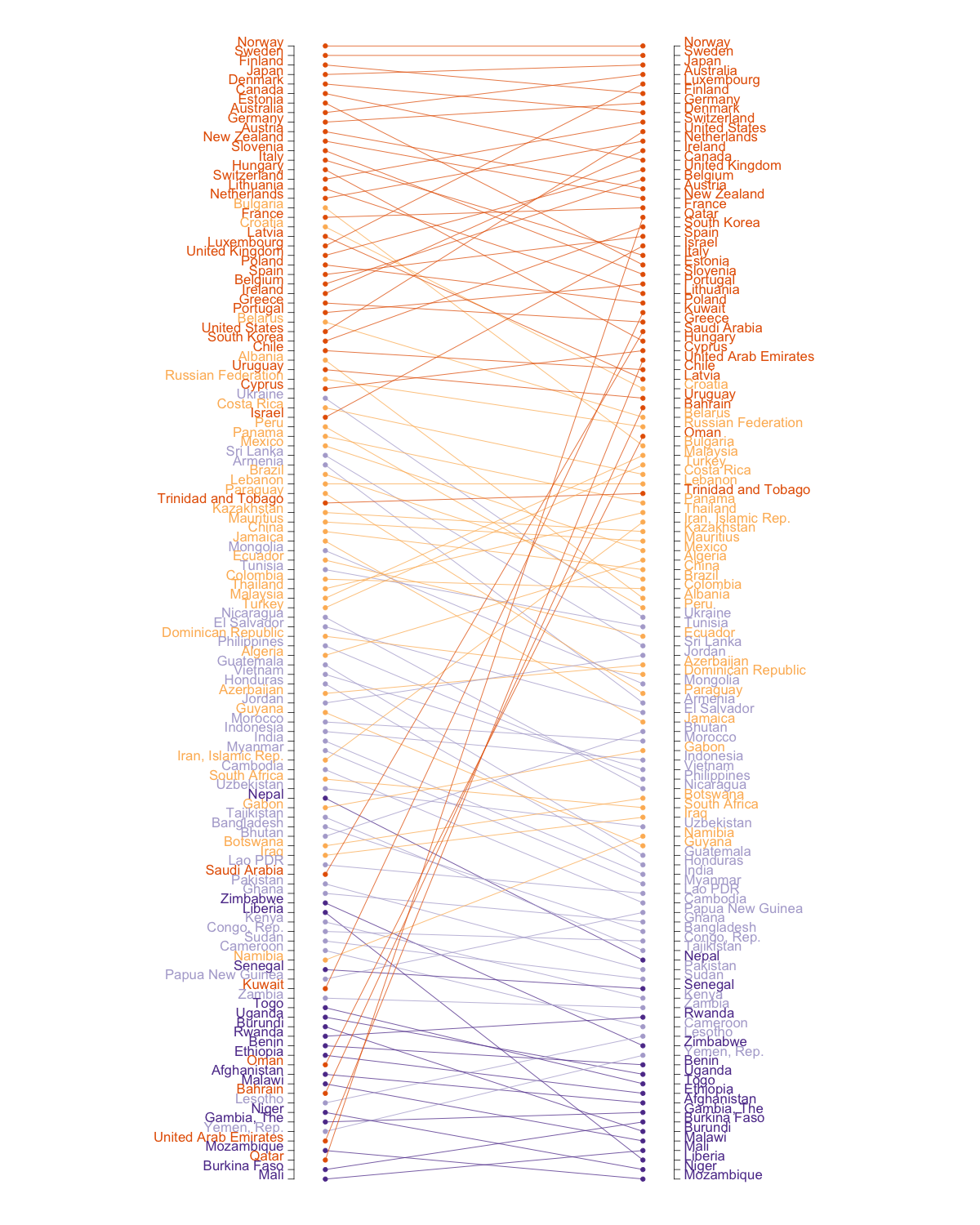
Figure C.1: Ladder plot for (posterior median of) $H$’s between using MML and using GGHE as the treatment variable

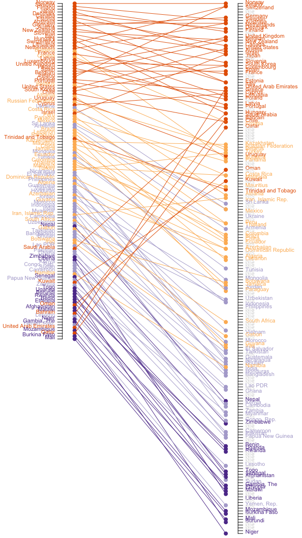
Figure C.2: Ladder plot for (posterior median of) latent $H$ ranking from LACSH using MML as the treatment variable against HDI ranking

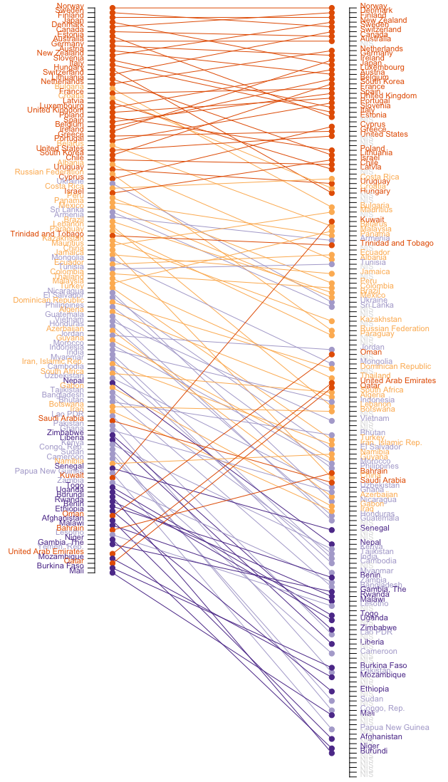
Figure C.3: Ladder plot for (posterior median of) latent $H$ ranking from LACSH using MML as the treatment variable against SPI ranking

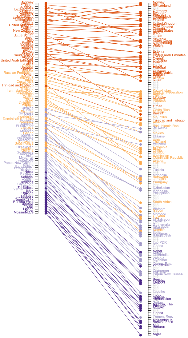
Figure C.4: Ladder plot for (posterior median of) latent $H$ ranking from LACSH using GGHE as the treatment variable against HDI ranking

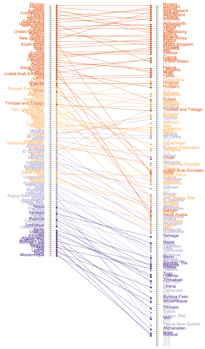
Figure C.5: Ladder plot for (posterior median of) latent $H$ ranking from LACSH using GGHE as the treatment variable against SPI ranking

Appendix D Diagnostics: Effective sample sizes

For model results, we utilised roughly 100,000 post-burn-in MCMC samples from the posterior distribution. Standard diagnostics suggested that each parameter of the MCMC chain had reached its steady state. We present trace plots for selected parameters from our LACSH models in the results in Table 5.1 in the main paper.

Moreover, to check convergence of our models, we calculate the effective sample size for each of the parameters. The effective sample size adjusts the total sample size due to autocorrelation, resulting in an approximate sample size that reflects what would have been an independent sample. Table D.1 shows the minimum and maximum effective sample size of all of the parameters calculated using the effectiveSize function in the coda package in R.

Table D.1: Minimum and maximum effective size of parameters for LACSH models

Models	Minimum effective sample size	Maximum effective sample size
MML as treatment	256.04	126927.2
GGHE as treatment	542.06	385777.8

Appendix E Additional interesting results on parameters

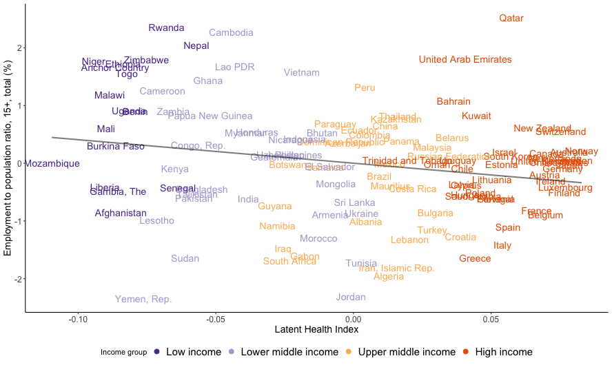
Figure E.1: Plot of employment-to-population ratio vs. posterior median of latent health, with GGHE as treatment and with a least squares regression fit for visualization

Figure E.1 shows a negative relationship for employment-to-population ratio and countries’ latent health, conditioned on other metrics with GGHE as treatment (90% credible interval for $a_{2}$ is $(-6.53,-0.90)$). The relevant discussions appear in Section 5.3.

Additionally, with GGHE as treatment, the metric ‘renewable energy consumption’ (shown in Figure E.2 and discussed in Section 6.3) also has a negative relationship with the country’s latent health (90% credible interval for $a_{15}$ is $(-13.64,-8.26)$).

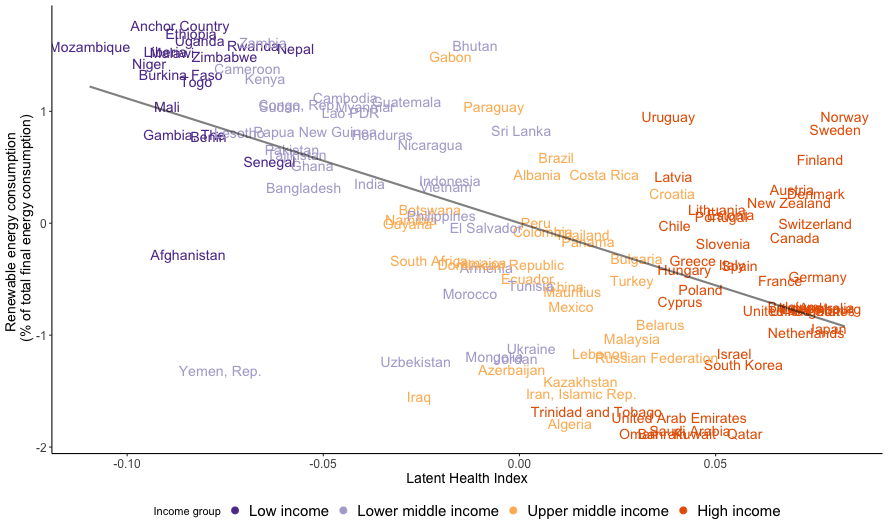
Figure E.2: Plot of renewable energy consumption vs. posterior median of latent health, with GGHE as treatment and with a least squares regression fit for visualization

There are a few possible explanations for this negative relationship. For example, lower-income countries lack the capital to expand existing infrastructure for electricity access, especially into rural areas, hence certain renewable energy sources that do not rely on existing infrastructure serve as more viable options. In addition, high-income countries may be reluctant, for various reasons, to transition from established infrastructure to renewable energy sources.

Appendix F Posterior average dose-response curves for subsample of countries

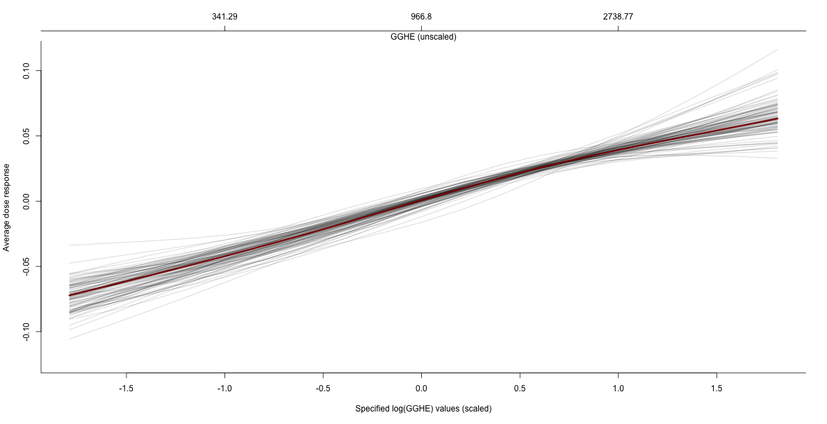
Figure F.1: Posterior median dose-response function (red), with GGHE as treatment, for the subsample of 82 countries, with 100 thinned MCMC samples (gray) for visualization of uncertainty

Figure F.1 shows the average dose-response curves for 82 countries, a subsample of the original set of 120 countries. Subsampling was done to address the consistent pattern of covariate imbalance in Figure 10. Compared to using the full sample, the average dose-response curve for the subsample shows less uncertainty with tighter credible bands for the dose-response curve, but the MCMC samples are no longer always monotone.

Figure F.2: Plot of p-values (reversed-scale) for assessing covariate balance, with GGHE as treatment, for the subsample of 82 countries

Figure F.2 no longer shows any consistent pattern of covariate imbalance.

Appendix G Simulation studies

G.1 Simulation study I: Cross validation study

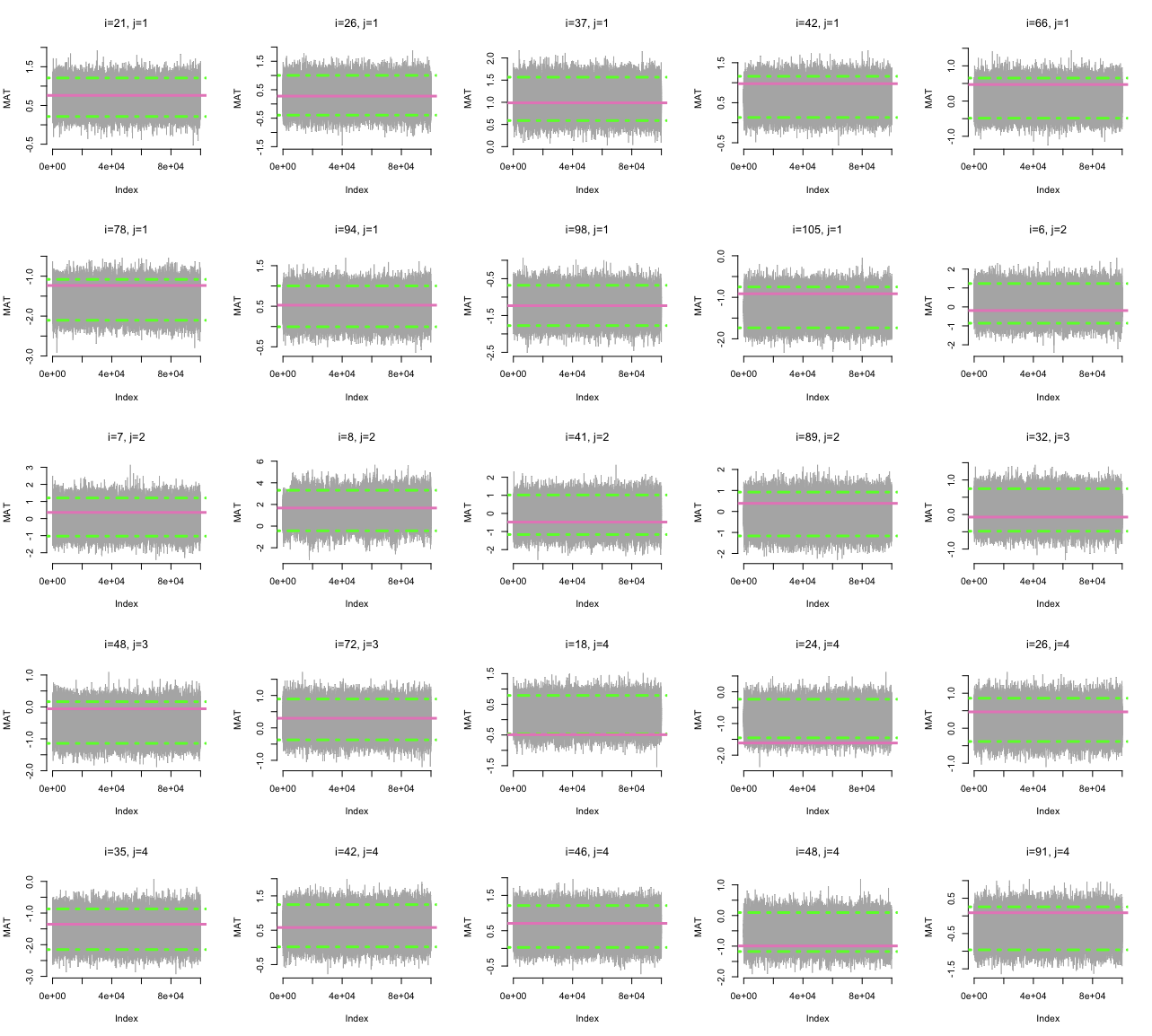
Figure G.1: Trace plots of the corresponding missing $y_{ij}$’s for a chosen iteration to be representative of all 10 iterations. The green dashed lines are 95% posterior predictive intervals and the red lines represent the true $y_{ij}$’s before withholding them as missing. We find that across the 10 iterations, the lowest capture rate for missing $y_{ij}$’s values is 90% and the highest capture rate is 98%.

Table G.1: ‘Capture’ rate for 100 missing $y_{ij}$ values using a 95% posterior predictive interval for each of the 10 iterations. For each iteration, we determine how many times (out of 100) the true value was ‘captured’ by the intervals, and tabulate the rates of capture in this table.

Iteration	$1$	$2$	$3$	$4$	$5$	$6$	$7$	$8$	$9$	$10$
Capture rate	$0.90$	$0.98$	$0.91$	$0.92$	$0.93$	$0.90$	$0.98$	$0.92$	$0.90$	$0.92$

G.2 Simulation study II: Recovering parameter values from fictitious data

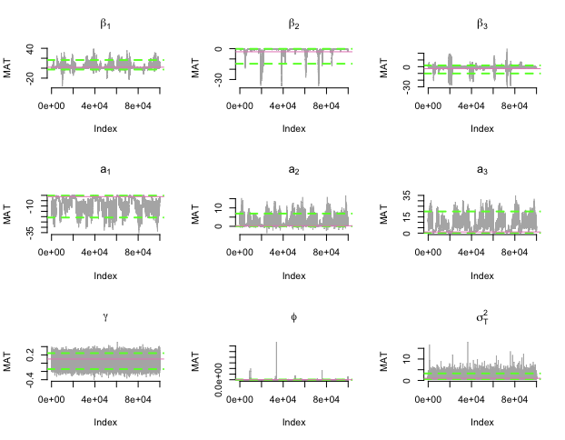
Figure G.2: Trace plots of the corresponding parameters for a chosen iteration (iteration 21 out of 50) for $\bm{\beta}=\{2,-3,-3\}$. The green dashed lines are 95% credible intervals and the red lines represent the true parameter values.

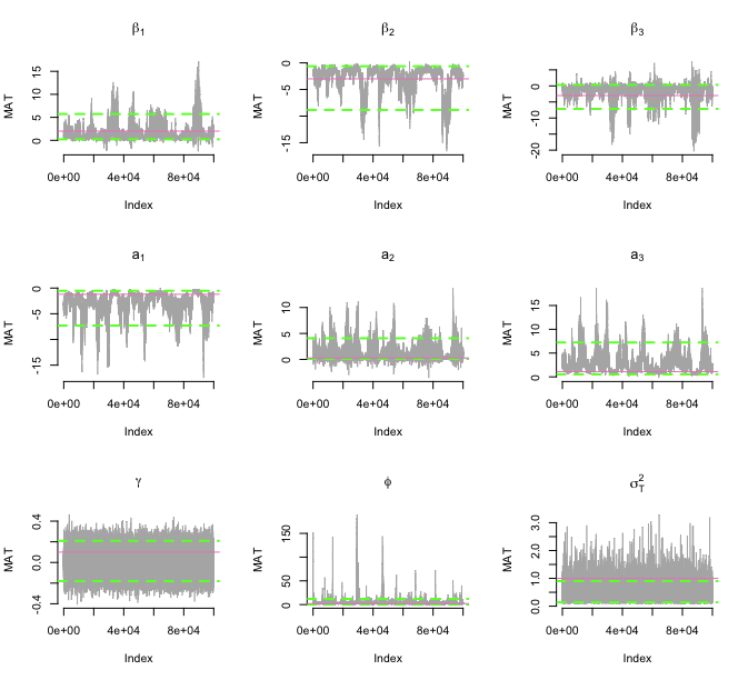
Figure G.3: Trace plots of the corresponding parameters for a chosen iteration (iteration 24 out of 50) for $\bm{\beta}=\{2,-3,-3\}$. The green dashed lines are 95% credible intervals and the red lines represent the true parameter values.

Table G.2: ‘Capture’ rate for each parameter using a 95% credible interval over 50 iterations. For each iteration, the LACSH model was fitted to the randomly generated $H$’s and $Y$’s. For each model parameter, we determine how many times the true value was ‘captured’ by the fifty 95% credible intervals, and tabulate the rates of capture in this table.

	Parameter	$\bm{\beta}=\{2,3,3\}$	$\bm{\beta}=\{2,-3,\frac{(-\beta_{0}+\beta_{1}\bar{T})}{R}\}$	$\bm{\beta}=\{2,-3,-3\}$
1	$a_{1}$	$0.84$	$0.70$	$0.82$
2	$a_{2}$	$0.86$	$0.74$	$0.86$
3	$a_{3}$	$0.86$	$0.72$	$0.80$
4	$\beta_{1}$	$0.90$	$1$	$0.92$
5	$\beta_{2}$	$0.80$	$0.68$	$0.82$
6	$\beta_{3}$	$0.94$	$0.72$	$0.72$
7	$\gamma$	$1$	$1$	$1$
8	$\phi$	$0.86$	$0.96$	$0.90$
9	$\sigma^{2}_{H}$	$0.90$	$0.84$	$0.86$
10	$\sigma^{2}_{T}$	$0.94$	$0.90$	$0.92$
11	$\Sigma_{y[1,1]}$	$0.90$	$0.96$	$0.92$
12	$\Sigma_{y[1,2]}$	$0.98$	$0.94$	$0.96$
13	$\Sigma_{y[1,3]}$	$0.88$	$0.88$	$0.90$
14	$\Sigma_{y[2,2]}$	$0.94$	$0.90$	$0.96$
15	$\Sigma_{y[2,3]}$	$1$	$0.98$	$0.94$
16	$\Sigma_{y[3,3]}$	$0.86$	$0.80$	$0.82$

References

- An [2010] An, W. (2010). “4. Bayesian Propensity Score Estimators: Incorporating Uncertainties in Propensity Scores into Causal Inference.” Sociological Methodology, 40(1): 151–189.
- Banerjee [2005] Banerjee, S. (2005). “On geodetic distance computations in spatial modeling.” Biometrics, 61(2): 617–625.
-
Center for Systemic Peace [2016]
Center for Systemic Peace (2016).
“The Polity Project.”
URL http://www.systemicpeace.org/polityproject.html - Chapman et al. [2008] Chapman, B., Higgins, T., Lin, L., et al. (2008). “Sharing the costs of parental leave: Paid parental leave and income contingent loans.” Information Paper (Committee for Economic Development of Australia), iv.
- Chiu et al. [2011] Chiu, G. S., Guttorp, P., Westveld, A. H., Khan, S. A., and Liang, J. (2011). “Latent health factor index: A statistical modeling approach for ecological health assessment.” Environmetrics, 22(3): 243–255.
- Chiu and Westveld [2011] Chiu, G. S. and Westveld, A. H. (2011). “A unifying approach for food webs, phylogeny, social networks, and statistics.” Proceedings of the National Academy of Sciences, 108(38): 15881–15886.
- Chiu et al. [2013] Chiu, G. S., Wu, M. A., and Lu, L. (2013). “Model-based assessment of estuary ecosystem health using the latent health factor index, with application to the Richibucto Estuary.” PloS one, 8(6): e65697.
- Cole and Frangakis [2009] Cole, S. R. and Frangakis, C. E. (2009). “The consistency statement in causal inference: a definition or an assumption?” Epidemiology, 20(1): 3–5.
- Conceição and Bandura [2008] Conceição, P. and Bandura, R. (2008). “Measuring subjective wellbeing: A summary review of the literature.” United nations development programme (UNDP) development studies, working paper.
- Darmofal [2015] Darmofal, D. (2015). Spatial analysis for the social sciences. Cambridge University Press.
- Gelfand et al. [2010] Gelfand, A. E., Diggle, P., Guttorp, P., and Fuentes, M. (2010). Handbook of spatial statistics. CRC press.
- Gelman and Hill [2007] Gelman, A. and Hill, J. (2007). Data analysis using regression and multilevel/hierarchical models, volume 1. Cambridge University Press New York, NY, USA.
- Gelman et al. [2014] Gelman, A., Hwang, J., and Vehtari, A. (2014). “Understanding predictive information criteria for Bayesian models.” Statistics and computing, 24(6): 997–1016.
- Gleditsch and Ward [2001] Gleditsch, K. S. and Ward, M. D. (2001). “Measuring space: A minimum-distance database and applications to international studies.” Journal of Peace Research, 38(6): 739–758.
- Hashimoto et al. [2018] Hashimoto, T., Oda, K., and Qi, Y. (2018). “On Well-being, Sustainability and Wealth Indices beyond GDP: A guide using cross-country comparisons of Japan, China, South Korea.” Economic Studies, 68(1): 35–88.
- Helliwell and Huang [2014] Helliwell, J. F. and Huang, H. (2014). “New measures of the costs of unemployment: Evidence from the subjective well-being of 3.3 million Americans.” Economic Inquiry, 52(4): 1485–1502.
- Hernán and Robins [2020] Hernán, M. and Robins, J. (2020). Causal inference. Boca Raton: Chapman & Hall/CRC, forthcoming.
- Hirano and Imbens [2004] Hirano, K. and Imbens, G. W. (2004). “The propensity score with continuous treatments.” Applied Bayesian modeling and causal inference from incomplete-data perspectives, 226164: 73–84.
- Hlavac [2022] Hlavac, M. (2022). “stargazer: beautiful LATEX, HTML and ASCII tables from R statistical output.” The Comprehensive R Archive Network.
- Hoeting et al. [2006] Hoeting, J. A., Davis, R. A., Merton, A. A., and Thompson, S. E. (2006). “Model selection for geostatistical models.” Ecological Applications, 16(1): 87–98.
- Hoff [2009] Hoff, P. D. (2009). A first course in Bayesian statistical methods, volume 580. Springer.
- Horrace [2005] Horrace, W. C. (2005). “Some results on the multivariate truncated normal distribution.” Journal of multivariate analysis, 94(1): 209–221.
- Imai and Van Dyk [2004] Imai, K. and Van Dyk, D. A. (2004). “Causal inference with general treatment regimes: Generalizing the propensity score.” Journal of the American Statistical Association, 99(467): 854–866.
- Imbens [2000] Imbens, G. W. (2000). “The role of the propensity score in estimating dose-response functions.” Biometrika, 87(3): 706–710.
- Imbens and Rubin [2015] Imbens, G. W. and Rubin, D. B. (2015). Causal inference in statistics, social, and biomedical sciences. Cambridge University Press.
- Jackman [2001] Jackman, S. (2001). “Multidimensional analysis of roll call data via Bayesian simulation: Identification, estimation, inference, and model checking.” Political Analysis, 9(3): 227–241.
- Kaplan and Chen [2012] Kaplan, D. and Chen, J. (2012). “A two-step Bayesian approach for propensity score analysis: Simulations and case study.” Psychometrika, 77(3): 581–609.
- Keele and Titiunik [2015] Keele, L. J. and Titiunik, R. (2015). “Geographic boundaries as regression discontinuities.” Political Analysis, 23(1): 127–155.
- Klugman et al. [2011] Klugman, J., Rodríguez, F., and Choi, H.-J. (2011). “The HDI 2010: new controversies, old critiques.” The Journal of Economic Inequality, 9(2): 249–288.
- Kluve et al. [2012] Kluve, J., Schneider, H., Uhlendorff, A., and Zhao, Z. (2012). “Evaluating continuous training programmes by using the generalized propensity score.” Journal of the Royal Statistical Society: Series A (Statistics in Society), 175(2): 587–617.
-
Kubiszewski et al. [2014]
Kubiszewski, I., Costanza, R., Franco, C., Lawn, P., Talberth, J., Jackson, T.,
and Aylmer, C. (2014).
“Beyond GDP: are there better ways to measure well-being?”
The Conversation.
URL https://theconversation.com/beyond-gdp-are-there-better-ways-to-measure-well-being-33414 - Kuh [2022] Kuh, F. S. (2022). “A Holistic Bayesian Framework for Modelling Latent Socio-Economic Health.” Ph.D. thesis, The Australian National University (Australia).
- Lea [1993] Lea, R. A. (1993). “World Development Report 1993:‘Investing in Health’.”
- Martin and Quinn [2002] Martin, A. D. and Quinn, K. M. (2002). “Dynamic ideal point estimation via Markov chain Monte Carlo for the US Supreme Court, 1953–1999.” Political Analysis, 10(2): 134–153.
- McCandless et al. [2010] McCandless, L. C., Douglas, I. J., Evans, S. J., and Smeeth, L. (2010). “Cutting feedback in Bayesian regression adjustment for the propensity score.” The international journal of biostatistics, 6(2).
- McCandless et al. [2009] McCandless, L. C., Gustafson, P., and Austin, P. C. (2009). “Bayesian propensity score analysis for observational data.” Statistics in medicine, 28(1): 94–112.
- McGillivray and Clarke [2006] McGillivray, M. and Clarke, M. (2006). Human well-being: Concepts and measures. United Nations University Press.
-
New Economics Foundation [2016]
New Economics Foundation (2016).
“Happy Planet Index 2016: Methods Paper.”
Technical report.
URL https://static1.squarespace.com/static/5735c421e321402778ee0ce9/t/578cc52b2994ca114a67d81c/1468843308642/Methods+paper_2016.pdf - Noreen [2018] Noreen, S. (2018). “Quantifying the Impact of Local SUTVA Violations in Spatiotemporal Causal Models.” Ph.D. thesis, Emory University.
-
OECD [2018]
OECD (2018).
“OECD.Stat.”
URL https://stats.oecd.org/ -