Matrix-Monotonic Optimization $-$ Part II: Multi-Variable Optimization

Abstract

In contrast to Part I of this treatise [1] that focuses on the optimization problems associated with single matrix variables, in this paper, we investigate the application of the matrix-monotonic optimization framework in the optimization problems associated with multiple matrix variables. It is revealed that matrix-monotonic optimization still works even for multiple matrix-variate based optimization problems, provided that certain conditions are satisfied. Using this framework, the optimal structures of the matrix variables can be derived and the associated multiple matrix-variate optimization problems can be substantially simplified. In this paper several specific examples are given, which are essentially open problems. Firstly, we investigate multi-user multiple-input multiple-output (MU-MIMO) uplink communications under various power constraints. Using the proposed framework, the optimal structures of the precoding matrices at each user under various power constraints can be derived. Secondly, we considered the optimization of the signal compression matrices at each sensor under various power constraints in distributed sensor networks. Finally, we investigate the transceiver optimization for multi-hop amplify-and-forward (AF) MIMO relaying networks with imperfect channel state information (CSI) under various power constraints. At the end of this paper, several simulation results are given to demonstrate the accuracy of the proposed theoretical results.

I Motivations

The deployment of multi-antenna arrays opened a door to effectively exploit spatial resources to improve energy efficiency and spectrum efficiency [1, 2, 3, 4, 5]. Meanwhile, the involved design variables are usually matrices instead of simple scalars [6, 7, 8]. In order to solve the matrix-variate optimization problems for MIMO communications efficiently, the most widely used logic is first to derive the optimal structures of the matrix variables. Then based on the optimal structures, the considered optimization problems can be greatly simplified [9, 10, 12, 15, 16, 11, 13, 14].

Matrix-monotonic optimization is an interesting framework that takes advantage of monotonic property in positive semidefinite matrix set to derive the optimal structures of optimization variables [1, 18, 17, 19, 20]. In Part I [1], we focus our attention on single-variable optimization problems. However, for many practical optimization problems there are multiple matrix variates to optimize. For example, in multi-user multiple-input multiple-output (MU-MIMO) communication systems, the transceiver optimization processes of the downlink and uplink involve multiple matrix variables, namely the equalizer matrices and precoder matrices [24, 23, 22, 21]. For multi-carrier MIMO systems, in each subcarrier there is a precoder matrix and an equalizer matrix [17]. Moreover, in multi-hop communications the forwarding matrix of each relay has to be optimized [25, 26].

This fact inspires us to take a further step and to investigate the optimization problems hinging on multiple matrix-variables. Generally speaking, solving an optimization problem having multiple matrix-variables is more challenging than its single matrix-variable counterpart. How to solve this kind of optimization problems has attracted substantial attention both across the wireless communication and signal processing research communities [21, 22, 23]. In contrast to single matrix-variable optimizations, for multiple matrix-variable optimization in most cases it is impossible to derive the optimal solutions in closed-form. Iterative optimization algorithms or alternating optimization algorithms have neeb widely used to solve this kind of optimization problems [23, 24, 27, 25, 26]. Unfortunately, there is no general-purpose mathematical tool or framework that can cover all the kinds of optimization problems. In some cases, similar to the single-variable case, for multiple matrix-variable optimization first the optimal structures of the matrix variables have to be derived, based on which the optimization can be significantly simplified and the corresponding convergence rate can be substantially improved.

In this paper, we investigate in detail, how to exploit the hidden monotonicity in positive semidefinite matrix fields to derive the optimal structures of the multiple matrix variables. Based on the optimal structures, the optimizations of multiple matrix variables can be significantly simplified. In our work, it is revealed that for many optimization problems associated with multiple matrix variables, the matrix-monotonic optimization framework still works. We also would like to point out that the authors of [17] also investigate how to apply matrix-monotonic optimization to optimization problems associated with multiple matrix variables. However, it is worth highlighting that the previous contribution [17] only considers a simple sum power constraint. By contrast, our work in this paper is significantly different from that in [17], since here diverse power constraints are taken into account, such as the multiple weighted power constraints of [20], the shaping constraint of [29, 28] and so on. Additionally, more scenarios are also taken into account. Furthermore, in addition to the multi-hop systems investigated in [17], in this paper, the MU-MIMO uplink and distributed sensor networks are also considered.

The main contributions of this paper are enumerated in the following. These contributions distinguish our work from the existing related works.

• Firstly, we investigate precoder optimization in the uplink of MU-MIMO communications under three different power constraints, namely the shaping constraint, joint power constraint and multiple weighted power constraints. Based on the matrix-monotonic optimization framework, the optimal structures of the matrix variables can be derived. Then the optimization can be substantially simplified and can be efficiently solved by an iterative algorithm. In each iteration based on the optimal structure, the optimal solutions of the remaining variables are standard water-filling solutions. We cover the precoder optimization under per-antenna power constraint as its special cases.

• Secondly, we investigate the signal compression matrix optimization problem in a distributed sensor network under the above three power constraints. For this data fusion optimization, there exist correlations between the signals transmitted from different sensors. This makes the corresponding optimization problem significantly different from that in the MU-MIMO uplink. Moreover, in contrast to [27], where at each sensor only the sum power constraint is considered, in our work more general power constraints are taken into account, namely the shaping constraint, joint power constraint and multiple weighted power constraints. This is our main contribution. Based on the matrix-monotonic optimization framework, the optimal structures of the compression matrices can be derived and the optimal solutions of the remaining vectors are found to correspond to water-filling solutions.

• Thirdly, we investigate the robust transceiver optimization problem of multi-hop amplify-and-forward (AF) cooperative MIMO networks, including both linear and nonlinear transceivers. For the linear transceivers, various kinds of performance metrics are taken into account, namely the additively Schur-convex and Schur-concave scenarios [25, 26, 30]. On the other hand, for nonlinear transceivers, both decision feedback equalizers (DFE) and Tomlinson-Harashima precoding (THP) are investigated. In contrast to [28, 31], various power constraints are taken into account in the robust transceiver optimization instead of the simple sum power constraint. Based on the proposed framework, the optimal structures of the robust transceiver design can be derived, based on which the robust transceiver optimization can be efficiently solved. Hence our contribution fills a void in the robust transceiver design literature of multi-hop AF MIMO systems under multiple weighted power constraints.

The remainder of this paper is organized as follows. In Section II, the basic properties of the framework on matrix-monotonic optimizations are given first. Following that, the MU-MIMO uplink is investigated in Section III. Compression matrix optimization for distributed sensor networks is discussed based on matrix-monotonic optimization in Section IV. In Section V, robust transceiver optimization is proposed for multi-hop AF MIMO relaying networks separately under shaping constraints, joint power constraints and multiple weighted power constraints. Several numerical results are given in Section VII, Finally, the conclusions are drawn in Section VIII.

Notation: To be consistent with our Part I work [1], the following notations and definitions are used throughout this paper. The symbols $\bm{Z}^{\rm H}$, $\bm{Z}^{\rm{T}}$, ${\rm Tr}(\bm{Z})$ and $|\bm{Z}|$ denote the Hermitian transpose, transpose, trace and determinant of matrix $\bm{Z}$, respectively. The matrix $\bm{Z}^{\frac{1}{2}}$ is the Hermitian square root of a positive semidefinite matrix $\bm{Z}$, which is also a positive semidefinite matrix. For an $N\times N$ matrix ${\bm{Z}}$, the vector ${\bm{\lambda}}({\bm{Z}})$ is defined as ${\bm{\lambda}}({\bm{Z}})=[\lambda_{1}({\bm{Z}}),\cdots,\lambda_{N}({\bm{Z}})]^{\rm{T}}$ where $\lambda_{i}(\bm{Z})$ denotes the $i$th largest eigenvalue of $\bm{Z}$. The symbol $[\bm{Z}]_{i,j}$ denotes the $i$th-row and $j$th-column element. On the other hand, the symbol $\bm{d}(\bm{Z})$ denotes the vector consisting of the diagonal elements of $\bm{Z}$. The identity matrix is denoted by $\bm{I}$. In this paper, $\bm{\Lambda}$ always represents a diagonal matrix, and $\bm{\Lambda}\searrow$ and $\bm{\Lambda}\nearrow$ represent a rectangular or square diagonal matrix with the diagonal elements in descending order and ascending order, respectively.

II Fundamentals of Matrix-Monotonic Optimization

In this paper, we investigate a real valued optimization problem with multiple complex matrix variables $\{\bm{X}_{k}\}_{k=1}^{K}$ which is generally formulated as

Opt. 1.1: $$\min\limits_{\{\bm{X}_{k}\}_{k=1}^{K}}f_{0}(\{\bm{X}_{k}\}_{k=1}^{K}),$$

$$\ \ \ {\rm{s.t.}}\ \ \ \ \psi_{k,i}(\bm{X}_{k})\leq 0,$$

$$\ \ \ \ \ \ \ \ \ \ \ 1\leq k\leq K,1\leq i\leq I_{k},$$ (1)

where $\psi_{k,i}(\cdot)$, $1\leq k\leq K$, $1\leq i\leq I_{k}$, denotes the constraint functions. Similar to the single-variate matrix-monotonic optimization investigated in Part I [1], all constraints considered in this paper are right unitarily invariant, i.e., for arbitrary unitary matrices ${\bm{Q}}_{\bm{X}_{k}}$’s,

$$\psi_{k,i}\left(\bm{X}_{k}{\bm{Q}}_{\bm{X}_{k}}\right)=\psi_{k,i}\left(\bm{X}_{k}\right).$$ (2)

In the following, several specific power constraints are given. The general power constraint model is one of the main contributions of this work.

II-A The Constraints on Multiple Matrix Variables

The simplest constraint is sum power constraint, i.e., the sum power across all transmit antennas is smaller than a predefined threshold. For example, in MU-MIMO uplink communications, each mobile terminal has a sum power constraint such as

$${\rm Tr}\big{(}\bm{X}_{k}\bm{X}_{k}^{\rm H}\big{)}\leq P_{k}.$$ (3)

It is obvious that the sum power constraint is right unitarily invariant. Moreover, in order to constrain the fluctuation of the eigenvalues of $\bm{X}_{k}\bm{X}_{k}^{\rm H}$, the following joint power constraint will be used [28, 29]

$${\rm Tr}\big{(}\bm{X}_{k}\bm{X}_{k}^{\rm H}\big{)}\leq P_{k},\ \ \bm{X}_{k}\bm{X}_{k}^{\rm H}\preceq\tau_{k}\bm{I}.$$ (4)

The difference between the sum power constraint and the joint power constraint is that there is an additional maximum eigenvalue constraint. It is obvious that the joint power constraint is right unitarily invariant.

From the circuit viewpoint, each amplifier is connected to one distinct antenna. It is not reasonable to use the sum power as a constraint as the powers cannot be shared between different antennas. In other words, the individual power constraint or per-antenna power constraint is more practical, which is formulated as [31, 32, 21]

$$\big{[}\bm{X}_{k}\bm{X}_{k}^{\rm H}\big{]}_{n,n}\leq P_{k,n},\ \ n=1,\cdots,N.$$ (5)

The per-antenna power constraint is also right unitarily invariant. It is worth highlighting that the per-antenna power constraint cannot include the sum power constraint as its special case.

In order to build a more general constraint model including more specific power constraints as its special cases, multiple weighted power constraints are given in the following [1, 20]

$${\rm Tr}\big{(}\bm{\Omega}_{k,i}\bm{X}_{k}\bm{X}_{k}^{\rm H}\big{)}\leq P_{k,i},\ \ i=1,\cdots,I_{k},$$ (6)

where $I_{k}$ is the number of weighted power constraints for the $k$th variable ${\bm{X}}_{k}$. The positive semidefinite matrices $\bm{\Omega}_{k,i}$’s are weighting matrices. The multiple weighted power constraints are right unitarily invariant as well.

Finally, in order to constrain the transmit signals to be in a desired region, shaping constraint can be used. Shaping constraint is a constraint on the covariance matrix of transmitted signals. Specifically, the shaping constraint on a matrix variable $\bm{X}_{k}$ is defined as [28, 33]

$$\bm{X}_{k}\bm{X}_{k}^{\rm H}\preceq\bm{R}_{{\rm s}_{k}},$$ (7)

where $\bm{R}_{{\rm s}_{k}}$ is the desired signal shaping matrix [28, 33]. The shaping constraint (7) is right unitarily invariant as well. Under these power constraints, in the following we give the properties which are the basis of application of the framework of matrix-monotonic optimization.

From a mathematical perspective, the more complicated power constraints will significantly change the feasible set compared to that of the sum power constraint. This is because the sum power constraint is both right unitarily invariant and left unitarily invariant, however the general power constraints are only right unitarily invariant. In other words, the symmetry of sum power constraint does not exist for the general power constraints such as multiple weighted power constraints. It is clear that under multiple weighted power constraints the extreme values and the optimal solutions are significantly different from that under the sum power constraint. The multiple weighted power constraints model also includes the sum power constraint model as its special case. Note that the sum power constraint model is not a special case of the per-antenna power constraint model. One model can include two different constraint models as its special cases. This is also an advantage of the multiple weighted power constraints model.

II-B Matrix-Monotonic Properties

The framework of matrix-monotonic optimization aims at exploiting the monotonicity in positive semidefinite field to derive the optimal structures of the matrix variates. As the constraints in Opt. 1.1 are right unitarily invariant, defining $\bm{X}_{k}=\bm{F}_{k}{\bm{Q}}_{\bm{X}_{k}}$ Opt. 1.1 is equivalent to the following optimization problem

$$\textbf{Opt.\,1.2:}\ \ \min\limits_{\{\bm{F}_{k},{\bm{Q}}_{\bm{X}_{k}}\}_{k=1}^{K}}\ \ f_{0}(\{\bm{F}_{k}{\bm{Q}}_{\bm{X}_{k}}\}_{k=1}^{K}),$$

$${\rm{s.t.}}\ \ \ \ \psi_{k,i}(\bm{F}_{k})\leq 0,$$

$$1\leq k\leq K,1\leq i\leq I_{k}$$ (8)

In our work, Opt. 1.2: satisfies the following properties.

For the $k$th optimal unitary matrix ${\bm{Q}}_{\bm{X}_{k}}$, the objective function in Opt. 1.2 can be transferred into a function of ${\bm{\lambda}}(\bm{F}_{k}^{\rm H}\bm{\Pi}_{k}\bm{F}_{k})$ i.e.,

$$f_{0}(\{\bm{F}_{k}{\bm{Q}}_{\bm{X}_{k}}\}_{k=1}^{K})=g_{0,k}({\bm{\lambda}}(\bm{F}_{k}^{\rm H}\bm{\Pi}_{k}\bm{F}_{k})),\text{for}\ k=1,\cdots,K$$ (9)

with $g_{0,k}({\bm{\lambda}}(\bm{F}_{k}^{\rm H}\bm{\Pi}_{k}\bm{F}_{k}))$ being a monotonically decreasing function with respect to ${\bm{\lambda}}(\bm{F}_{k}^{\rm H}\bm{\Pi}_{k}\bm{F}_{k})$ for $k=1,\cdots,K$. The optimal $\bm{F}_{k}$ is a Pareto optimal solution of the following vector optimization subproblem

$$\textbf{Opt.\,1.3:}\ \ \max\limits_{\bm{F}_{k}}\ \ {\bm{\lambda}}(\bm{F}_{k}^{\rm H}\bm{\Pi}_{k}\bm{F}_{k}),$$

$${\rm{s.t.}}\ \ \ \ \psi_{k,i}(\bm{F}_{k})\leq 0,\ \ 1\leq i\leq I_{k},$$ (10)

which is equivalent to the following matrix-monotonic optimization problem [17, 1]

$$\textbf{Opt.\,1.4:}\ \ \max\limits_{\bm{F}_{k}}\ \ \bm{F}_{k}^{\rm H}\bm{\Pi}_{k}\bm{F}_{k},$$

$${\rm{s.t.}}\ \ \ \ \psi_{k,i}(\bm{F}_{k})\leq 0,\ \ 1\leq i\leq I_{k}.$$ (11)

where $\bm{\Pi}_{k}$ is independent of $\bm{F}_{k}$. Then, based on the results of Part I [1], the optimal structure of $\bm{F}_{k}$ can be derived. Based on the optimal structures, the optimization problem can be substantially simplified. To elaborate a little further, given the optimal structures, the optimization problem Opt. 1.2 associated with multiple matrix variables can be efficiently solved in an iterative manner. It is worth noting that given the optimal structures, an iterative algorithm is still needed to solve Opt. 1.2 and in most cases the iterative algorithms used are iterative water-filling algorithms [54, 53]. Suffice to say that the convergence of this kind of algorithms can be guaranteed, but in a general case after convergence only covergence to the local optimum of the final solutions can be guaranteed. Based on Part I [1], in the following the fundamental results for Opt. 1.4 are given, which constitute the basis for the following sections.

Shaping Constraint For the shaping constraint, Opt. 1.4 becomes the following optimization problem [28]

$$\textbf{Opt.\,1.5:}\ \ {\max}_{\bm{F}_{k}}\ \ \bm{F}_{k}^{\rm H}\bm{\Pi}_{k}\bm{F}_{k}$$

$${\rm s.t.}\ \bm{F}_{k}\bm{F}_{k}^{\rm H}\preceq\bm{R}_{\rm{s}_{k}}.$$ (12)

The following lemma reveals the optimal structure of $\bm{F}_{k}$ for Opt. 1.5 with the shaping constraint.

Lemma 1

When the rank of $\bm{R}_{\rm{s}_{k}}$ is not higher than the number of columns and the number of rows in $\bm{F}_{k}$, the optimal solution $\bm{F}_{\rm{opt},k}$ of Opt. 1.5 is a square root of $\bm{R}_{\rm{s}_{k}}$, i.e., $\bm{F}_{\rm{opt},k}\bm{F}_{\rm{opt},k}^{\rm H}=\bm{R}_{\rm{s}_{k}}$.

Joint Power Constraint Under the joint power constraint, Opt. 1.4 can be rewritten as

$$\textbf{Opt.\,1.6:}\ \ {\max}_{\bm{F}_{k}}\ \bm{F}_{k}^{\rm H}\bm{\Pi}_{k}\bm{F}_{k}$$

$${\rm s.t.} {\rm Tr}\big{(}\bm{F}_{k}\bm{F}_{k}^{\rm H}\big{)}\leq P_{k},\bm{F}_{k}\bm{F}_{k}^{\rm H}\preceq\tau_{k}\bm{I}.$$ (13)

The Pareto optimal solution $\bm{F}_{\rm{opt},k}$ for Opt. 1.6 is given in Lemma 2.

Lemma 2

For Opt. 1.6 with the joint power constraint, the Pareto optimal solutions satisfy the following structure

$$\bm{F}_{\rm{opt},k}= \bm{U}_{\bm{\Pi}_{k}}\bm{\Lambda}_{\bm{F}_{k}}\bm{U}_{\text{Arb},k}^{\rm H},$$ (14)

where the unitary matrix $\bm{U}_{\bm{\Pi}_{k}}$ is specified by the EVD

$$\bm{\Pi}_{k}= \bm{U}_{\bm{\Pi}_{k}}\bm{\Lambda}_{\bm{\Pi}_{k}}\bm{U}_{\bm{\Pi}_{k}}^{\rm H}\ \text{with}\ \bm{\Lambda}_{\bm{\Pi}_{k}}\searrow,$$ (15)

every diagonal element of the rectangular diagonal matrix $\bm{\Lambda}_{\bm{F}_{k}}$ is smaller than $\sqrt{\tau_{k}}$, and $\bm{U}_{\text{Arb},k}$ is an arbitrary unitary matrix having the appropriate dimension.

Multiple Weighted Power Constraints Under the multiple weighted power constraints, Opt. 1.4 becomes

$$\textbf{Opt.\,1.7:}\max\limits_{\bm{F}_{k}}\ \ \bm{F}_{k}^{\rm H}\bm{\Pi}_{k}\bm{F}_{k}$$

$${\rm s.t.}\ \ {\rm Tr}\big{(}\bm{\Omega}_{k,i}\bm{F}_{k}\bm{F}_{k}^{\rm H}\big{)}\leq P_{k,i},1\leq i\leq I_{k}.$$ (16)

Note that the weighted power constraints include both the sum power constraint and per-antenna power constraints as its special cases. The Pareto optimal solution $\bm{F}_{\rm{opt},k}$ for Opt. 1.7 is given in Lemma 3.

Lemma 3

The Pareto optimal solutions of Opt. 1.6 satisfy the following structure

$$\bm{F}_{\rm{opt},k}= \bm{\Omega}_{k}^{-\frac{1}{2}}\bm{U}_{\widetilde{\bm{\Pi}}_{k}}\bm{\Lambda}_{\widetilde{\bm{F}}_{k}}\bm{U}_{\rm{Arb},k}^{\rm H},$$ (17)

where $\bm{U}_{\rm{Arb},k}$ is an arbitrary unitary matrix of appropriate dimension, $\bm{\Omega}_{k}=\sum_{i=1}^{I_{k}}\alpha_{k,i}\bm{\Omega}_{k,i}$, the nonnegative scalars $\alpha_{k,i}$ are the weighting factors that ensure that the constraints ${\rm Tr}\big{(}\bm{\Omega}_{k,i}\bm{F}_{k}\bm{F}_{k}^{\rm H}\big{)}\leq P_{k,i}$ hold and they can be computed by classic subgradient methods, while the unitary matrix $\bm{U}_{\widetilde{\bm{\Pi}}_{k}}$ is specified by the EVD

$$\bm{\Omega}_{k}^{-\frac{1}{2}}\bm{\Pi}_{k}\bm{\Omega}_{k}^{-\frac{1}{2}}= \bm{U}_{\widetilde{\bm{\Pi}}_{k}}\bm{\Lambda}_{\widetilde{\bm{\Pi}}_{k}}\bm{U}_{\widetilde{\bm{\Pi}}_{k}}^{\rm H}\ \text{with}\ \bm{\Lambda}_{\widetilde{\bm{\Pi}}_{k}}\searrow.$$ (18)

In this paper, we focus our attention on the optimization problems of multiple complex matrix variates. In order to overcome the difficulties arising from the coupling relationships among the multiple matrix variates, the right unitarily invariant property of the constraints in Opt. 1.1 is exploited to introduce a series of auxiliary unitary matrices. Each auxiliary unitary matrix aligns its corresponding matrix variable to achieve extreme objective values. As a result, the optimal solutions of the matrix variables are Pareto optimal solutions of a series of single-variate matrix monotonic optimization problems. Then the optimal structure of each matrix variable can be derived, based on which the original optimization problem can be solved efficiently in an iterative manner. In the following, three specific optimization problems will be investigated, namely transceiver optimization for the multi-user MIMO (MU-MIMO) uplink, signal compression for distributed sensor networks and transceiver optimizations for multi-hop amplify-and-forward (AF) MIMO relaying networks. Generally speaking, an auxiliary unitary matrix aligns its lefthand side and righthand side with its corresponding matrix variables. The three examples are specifically chosen for characterizing the effects of the matrix variates on the auxiliary unitary matrices. Specifically, in the transceiver optimization of the MU-MIMO uplink, when optimizing the $k$th matrix variate, the other matrix variates only affect the righthand side of the corresponding unitary matrix. As for signal compression in distributed sensor networks, when optimizing the $k$th matrix variate, the effects of other matrix variates are only on the lefthand side of the corresponding unitary matrix. Finally, as for transceiver optimizations in AF MIMO relaying networks, when optimizing the $k$th matrix variate, the other matrix variates affect both sides of the corresponding unitary matrix.

III MU-MIMO Uplink Communications

The first application scenario for the matrix monotonic optimization theory is found in MU MIMO uplink communications. In the MU MIMO uplink system of Fig. 1, $K$ multi-antenna aided mobile users communicate with a multi-antenna assisted base station (BS) [34, 35, 36, 37]. The BS recovers the signals transmitted from all the $K$ mobile terminals. The sum rate maximization problem associated with this MU-MIMO uplink can be formulated as follows [21, 34, 35, 36]

$$\begin{array}[]{lcl}\textbf{Opt.\,2.1:}\!\!&\!\!\!\!\min\limits_{\{\bm{P}_{k}\}_{k=1}^{K}}\!\!\!\!&\!\!\!\!-\log\bigg{|}\bm{R}_{\rm n}+\sum\limits_{k=1}^{K}\bm{H}_{k}\bm{X}_{k}{\bm{W}}_{k}\bm{X}_{k}^{\rm H}\bm{H}_{k}^{\rm H}\bigg{|},\\ \!\!\!\!&\!\!\!\!\rm{s.t.}\!\!\!\!&\!\!\!\!\psi_{k,i}(\bm{X}_{k})\leq 0,1\leq i\leq I_{k},1\leq k\leq K,\end{array}\!\!$$ (21)

where $\bm{H}_{k}$ is the MIMO channel matrix between the $k$th user and the BS, $\bm{X}_{k}$ is the precoding matrix at the $k$th user, and $\bm{R}_{\rm n}$ is the additive noise’s covariance matrix at the BS. For the $k$th user, the positive definite matrix $\bm{W}_{k}$ is the corresponding weighting matrix. Different from the work in [21], the power constraints considered in our work are more general than the per-antenna power constraints in [21]. Similar to Opt. 1.2, defining $\bm{X}_{k}=\bm{F}_{k}{\bm{Q}}_{\bm{X}_{k}}$, the optimization problem (21) is equivalent to

$$\begin{array}[]{lcl}\textbf{Opt.\,2.2:}\!\!\!\!&\!\!\!\!\min\limits_{\{\bm{F}_{k}\}_{k=1}^{K}}\!\!\!\!&\!\!\!\!-\log\bigg{|}\bm{R}_{\rm n}+\sum\limits_{k=1}^{K}\bm{H}_{k}\bm{F}_{k}{\bm{Q}}_{\bm{X}_{k}}{\bm{W}}_{k}{\bm{Q}}_{\bm{X}_{k}}^{\rm{H}}\bm{F}_{k}^{\rm H}\bm{H}_{k}^{\rm H}\bigg{|},\\ \!\!\!\!&\!\!\!\!\rm{s.t.}\!\!\!\!&\!\!\!\!\psi_{k,i}(\bm{F}_{k})\leq 0,1\leq i\leq I_{k},1\leq k\leq K,\end{array}\!\!$$ (24)

The objective function of Opt. 2.2 satisfies the following property, which can be exploited to optimize the multiple

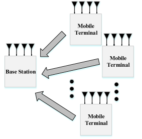
Figure 1: The uplink of MU-MIMO communications.

matrix variables

$$\log\bigg{|}\bm{R}_{\rm n}+\sum\limits_{k=1}^{K}\bm{H}_{k}\bm{F}_{k}{\bm{Q}}_{\bm{X}_{k}}\bm{W}_{k}{\bm{Q}}_{\bm{X}_{k}}^{\rm{H}}\bm{F}_{k}^{\rm H}\bm{H}_{k}^{\rm H}\bigg{|}$$

$$=\log\bigg{|}\bm{I}+\bm{H}_{k}\bm{F}_{k}{\bm{Q}}_{\bm{X}_{k}}\bm{W}_{k}{\bm{Q}}_{\bm{X}_{k}}^{\rm{H}}\bm{F}_{k}^{\rm H}\bm{H}_{k}^{\rm H}$$

$$\ \ \ \ \ \ \ \ \ \ \ \ \ \ \ \times\bigg{(}\bm{R}_{\rm n}+\sum\limits_{j\neq k}\bm{H}_{j}\bm{F}_{j}{\bm{Q}}_{\bm{X}_{k}}\bm{W}_{j}{\bm{Q}}_{\bm{X}_{k}}^{\rm{H}}\bm{F}_{j}^{\rm H}\bm{H}_{j}^{\rm H}\bigg{)}^{-1}\bigg{|}$$

$$+\log\bigg{|}\bm{R}_{\rm n}+\sum\limits_{j\neq k}\bm{H}_{j}\bm{F}_{j}{\bm{Q}}_{\bm{X}_{j}}\bm{W}_{j}{\bm{Q}}_{\bm{X}_{j}}^{\rm{H}}\bm{F}_{j}^{\rm H}\bm{H}_{j}^{\rm H}\bigg{|}$$

$$=\log\bigg{|}\bm{I}+\bm{W}_{k}{\bm{Q}}_{\bm{X}_{k}}^{\rm{H}}\bm{F}_{k}^{\rm H}\bm{H}_{k}^{\rm H}\bm{K}_{{\rm n}_{k}}^{-1}\bm{H}_{k}\bm{F}_{k}{\bm{Q}}_{\bm{X}_{k}}\bigg{|}+\log\big{|}\bm{K}_{{\rm n}_{k}}\big{|},$$ (25)

where we have

$$\bm{K}_{{\rm n}_{k}}= \bm{R}_{\rm n}+\sum\nolimits_{j\neq k}\bm{H}_{j}\bm{F}_{j}{\bm{Q}}_{\bm{X}_{j}}\bm{W}_{j}{\bm{Q}}_{\bm{X}_{j}}^{\rm{H}}\bm{F}_{j}^{\rm H}\bm{H}_{j}^{\rm H}.$$ (26)

Therefore, based on (III) for the $k$th matrix variate $\bm{F}_{k}$ Opt. 2.2 can be written in the following equivalent formula

$$\begin{array}[]{lcl}\textbf{Opt.\,2.3:}&\min\limits_{\bm{F}_{k}}&-\log\bigg{|}\bm{I}+\bm{W}_{k}{\bm{Q}}_{\bm{X}_{k}}^{\rm{H}}\bm{F}_{k}^{\rm H}\bm{H}_{k}^{\rm H}\bm{K}_{{\rm n}_{k}}^{-1}\bm{H}_{k}\bm{F}_{k}{\bm{Q}}_{\bm{X}_{k}}\bigg{|},\\ &\rm{s.t.}&\bm{K}_{{\rm n}_{k}}=\bm{R}_{\rm n}+\sum\limits_{j\neq k}\bm{H}_{j}\bm{F}_{j}{\bm{Q}}_{\bm{X}_{j}}\bm{W}_{j}{\bm{Q}}_{\bm{X}_{j}}^{\rm{H}}\bm{F}_{j}^{\rm H}\bm{H}_{j}^{\rm H},\\ &&\psi_{k,i}(\bm{F}_{k})\leq 0,i=1,\cdots,I_{k}.\end{array}$$ (30)

The matrix $\bm{F}_{k}^{\rm H}\bm{H}_{k}^{\rm H}\bm{K}_{{\rm n}_{k}}^{-1}\bm{H}_{k}\bm{F}_{k}$ can be interpreted as the matrix version SNR for the $k$th user [31]. Based on Matrix Inequality 4 in Part I [1], we have

$$\log\bigg{|}\bm{I}+\bm{W}_{k}{\bm{Q}}_{\bm{X}_{k}}^{\rm{H}}\bm{F}_{k}^{\rm H}\bm{H}_{k}^{\rm H}\bm{K}_{{\rm n}_{k}}^{-1}\bm{H}_{k}\bm{F}_{k}{\bm{Q}}_{\bm{X}_{k}}\bigg{|}$$

$$\leq\sum_{i}\log\left(1+\lambda_{i}(\bm{W})\lambda_{i}(\bm{F}_{k}^{\rm H}\bm{H}_{k}^{\rm H}\bm{K}_{{\rm n}_{k}}^{-1}\bm{H}_{k}\bm{F}_{k})\right).$$ (31)

The equality holds when the unitary matrix ${\bm{Q}}_{\bm{X}_{k}}$ equals

$${\bm{Q}}_{{\rm{opt}},\bm{X}_{k}}={\bm{U}}_{{\rm{SNR}},k}{\bm{U}}_{\bm{W}}^{\rm{H}}$$ (32)

where the unitary matrices ${\bm{U}}_{{\rm{SNR}},k}$ and ${\bm{U}}_{\bm{W}_{k}}$ are defined based on the following EVDs

$$\bm{F}_{k}^{\rm H}\bm{H}_{k}^{\rm H}\bm{K}_{{\rm n}_{k}}^{-1}\bm{H}_{k}\bm{F}_{k}={\bm{U}}_{{\rm{SNR}},k}{\bm{\Lambda}}_{{\rm{SNR}},k}{\bm{U}}_{{\rm{SNR}},k}^{\rm{H}}\text{ with }\bm{\Lambda}_{{\rm{SNR}},k}\searrow$$

$$\bm{W}_{k}=\bm{U}_{\bm{W}_{k}}\bm{\Lambda}_{\bm{W}_{k}}\bm{U}_{\bm{W}_{k}}^{\rm H}\text{ with }\bm{\Lambda}_{\bm{W}_{k}}\searrow.$$ (33)

From the multi-objective optimization viewpoint, the optimal solutions of Opt. 2.3 belong to the Pareto optimal solution sets of the following optimization problems for $1\leq k\leq K$

$$\begin{array}[]{lcl}\textbf{Opt.\,2.4:}&\max\limits_{\bm{F}_{k}}&{\bm{\lambda}}\left(\bm{F}_{k}^{\rm H}\bm{H}_{k}^{\rm H}\bm{K}_{{\rm n}_{k}}^{-1}\bm{H}_{k}\bm{F}_{k}\right),\\ &\rm{s.t.}&\bm{K}_{{\rm n}_{k}}=\bm{R}_{\rm n}+\sum\limits_{j\neq k}\bm{H}_{j}\bm{F}_{j}{\bm{Q}}_{\bm{X}_{j}}\bm{W}_{j}{\bm{Q}}_{\bm{X}_{j}}^{\rm{H}}\bm{F}_{j}^{\rm H}\bm{H}_{j}^{\rm H},\\ &&\psi_{k,i}(\bm{F}_{k})\leq 0,i=1,\cdots,I_{k}.\end{array}$$ (37)

which is equivalent to

$$\begin{array}[]{lcl}\textbf{Opt.\,2.5:}&\max\limits_{\bm{F}_{k}}&\bm{F}_{k}^{\rm H}\bm{H}_{k}^{\rm H}\bm{K}_{{\rm n}_{k}}^{-1}\bm{H}_{k}\bm{F}_{k},\\ &\rm{s.t.}&\bm{K}_{{\rm n}_{k}}=\bm{R}_{\rm n}+\sum\limits_{j\neq k}\bm{H}_{j}\bm{F}_{j}{\bm{Q}}_{\bm{X}_{j}}\bm{W}_{j}{\bm{Q}}_{\bm{X}_{j}}^{\rm{H}}\bm{F}_{j}^{\rm H}\bm{H}_{j}^{\rm H},\\ &&\psi_{k,i}(\bm{F}_{k})\leq 0,i=1,\cdots,I_{k}.\end{array}$$ (41)

It can be seen that by using alternating optimization algorithm, the multiple-matrix-variate optimization of Opt. 2.3 is transferred into the multiple single-matrix-variate matrix-monotonic optimization of Opt. 2.5. Based on Opt. 2.5, the optimal structure of $\bm{F}_{k}$ can be derived, and then the original optimization problem Opt. 2.2 can be solved in an iterative manner. It is worth noting that in most cases, for the alternating optimization algorithm, the final solutions are suboptimal. The alternating optimization algorithm stops when the performance improvement is smaller than a predefined threshold or the iteration number reaches the predefined maximum value. The convergence can be guaranteed when the subproblems are solved with global optimality.

1) Shaping Constraint: We have $I_{k}=1$ and

$$\psi_{k,1}(\bm{F}_{k})= \bm{F}_{k}\bm{F}_{k}^{\rm H}-\bm{R}_{{\rm s}_{k}}.$$ (42)

Based on Lemma 1 in Section II, we readily conclude that for $1\leq k\leq K$, when the rank of $\bm{R}_{{\rm s}_{k}}$ is not higher than the number of columns and the number of rows in $\bm{F}_{k}$, the optimal solution $\bm{F}_{{\rm opt},k}$ of Opt. 2.3 is a square root of $\bm{R}_{{\rm s}_{k}}$.

2) Joint Power Constraint: We have $I_{k}=2$ and

$$\begin{array}[]{l}\psi_{k,1}(\bm{F}_{k})={\rm Tr}\big{(}\bm{F}_{k}\bm{F}_{k}^{\rm H}\big{)}-P_{k},\\ \psi_{k,2}(\bm{F}_{k})=\bm{F}_{k}\bm{F}_{k}^{\rm H}-\tau_{k}\bm{I}.\end{array}$$ (45)

Based on Lemma 2 in Section II, we readily conclude that for $1\leq k\leq K$, the optimal solution $\bm{F}_{{\rm opt},k}$ of Opt. 2.3 satisfies the following structure

$$\bm{F}_{{\rm opt},k}= \bm{V}_{\widetilde{\bm{H}}_{k}}\bm{\Lambda}_{\bm{F}_{k}}\bm{U}_{{\rm{Arb}},k}^{\rm H},$$ (46)

where the unitary matrix $\bm{V}_{\widetilde{\bm{H}}_{k}}$ is defined based on the SVD

$$\bm{K}_{{\rm n}_{k}}^{-\frac{1}{2}}\bm{H}_{k}= \bm{U}_{\widetilde{\bm{H}}_{k}}\bm{\Lambda}_{\widetilde{\bm{H}}_{k}}\bm{V}_{\widetilde{\bm{H}}_{k}}^{\rm H}\text{ with }\bm{\Lambda}_{\widetilde{\bm{H}}_{k}}\searrow.$$ (47)

and every diagonal element of the rectangular diagonal matrix $\bm{\Lambda}_{\bm{F}_{k}}$ is smaller than $\sqrt{\tau_{k}}$. The diagonal matrix $\bm{\Lambda}_{\bm{F}_{k}}$ can be efficiently solved using a variant water-filling algorithm [52, 54].

3) Multiple Weighted Power Constraints: In this case, we have

$$\psi_{k,i}(\bm{F}_{k})= {\rm Tr}\big{(}\bm{\Omega}_{k,i}\bm{F}_{k}\bm{F}_{k}^{\rm H}\big{)}-P_{k,i}.$$ (48)

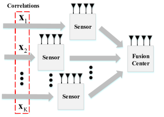
Figure 2: Illustration of distribute sensor network.

Then based on Lemma 3 in Section II, we conclude that for $1\leq k\leq K$, the optimal solution $\bm{F}_{{\rm opt},k}$ of Opt. 2.3 satisfies the following structure

$$\bm{F}_{{\rm opt},k}= \bm{\Omega}_{k}^{-\frac{1}{2}}\bm{V}_{\bm{\mathcal{H}}_{k}}\bm{\Lambda}_{\widetilde{\bm{F}}_{k}}\bm{U}_{{\rm{Arb}},k}^{\rm H},$$ (49)

where the unitary matrix $\bm{V}_{\bm{\mathcal{H}}_{k}}$ is defined by the following SVD

$$\bm{K}_{{\rm n}_{k}}^{-\frac{1}{2}}\bm{H}_{k}\bm{\Omega}_{k}^{-\frac{1}{2}}= \bm{U}_{\bm{\mathcal{H}}_{k}}\bm{\Lambda}_{\bm{\mathcal{H}}_{k}}\bm{V}_{\bm{\mathcal{H}}_{k}}^{\rm H}\text{ with }\bm{\Lambda}_{\bm{\mathcal{H}}_{k}}\searrow,$$ (50)

and the matrix $\bm{\Omega}_{k}$ is defined as

$$\bm{\Omega}_{k}= \sum\nolimits_{i=1}^{I_{k}}\alpha_{k,i}\bm{\Omega}_{k,i}.$$ (51)

The diagonal matrix $\bm{\Lambda}_{\widetilde{\bm{F}}_{k}}$ can be efficiently solved using water-filling algorithms [53].

IV Signal Compression for Distributed Sensor Networks

In the distributed sensor network illustrated in Fig. 2, the $K$ sensors transmit their individual signals to the fusion center [39, 40, 38, 44, 46, 42, 43, 47, 45, 41]. Specifically, the $k$th sensor transmits its signal $\bm{x}_{k}$ to the fusion center, when the channel between the $k$th sensor and the fusion center is $\bm{H}_{k}$. The fusion center recovers the transmitted signals $\bm{x}_{k}$ for $1\leq k\leq K$. In contrast to the scenario of MU-MIMO communications, there exist correlations among $\bm{x}_{k}$ [27], and the correlation matrix is denoted by

$$\bm{C}_{\bm{x}}= \mathbb{E}\Big{\{}\big{[}\bm{x}_{1}^{\rm T}\cdots\bm{x}_{K}^{\rm T}\big{]}^{\rm T}\big{[}\bm{x}_{1}^{\rm T}\cdots\bm{x}_{K}^{\rm T}\big{]}^{*}\Big{\}}.$$ (37)

Note that the correlations among the signals make the optimization approach of this application totally different from that of the MU-MIMO application.

To maximize the mutual information between the received signal at the data fusion center and the signal to estimate, the signal compression can be formulated as Opt. 3.1 [27], given as

$$\textbf{Opt.\,3.1:}\min\limits_{\{\bm{X}_{k}\}_{k=1}^{K}} -\log\Big{|}\bm{C}_{\bm{x}}^{-1}$$

$$+{\rm diag}\Big{\{}\big{\{}\bm{X}_{k}^{\rm H}\bm{H}_{k}^{\rm H}\bm{R}_{\rm{n}_{k}}^{-1}\bm{H}_{k}\bm{X}_{k}\big{\}}_{k=1}^{K}\Big{\}}\Big{|},$$

$${\rm s.t.} \psi_{k,i}\big{(}\bm{X}_{k}\bm{R}_{\bm{x}_{k}}^{\frac{1}{2}}\big{)}\leq 0,~{}1\leq i\leq I_{k},1\leq k\leq K,$$ (38)

where $\bm{F}_{k}$ is the signal compression matrix at the $k$th sensor, $\bm{R}_{\bm{x}_{k}}$ is the covariance matrix of the signal $\bm{x}_{k}$ transmitted from the $k$th sensor, and $\bm{R}_{\rm{n}_{k}}$ is the covariance matrix of the additive noise $\bm{n}_{k}$ for the $k$th sensor signal received in its own time slot at the fusion center. Note that if all the sensors send signals at the same frequency, all the $\bm{R}_{\rm{n}_{k}}$ are identical. If the sensors use different frequency bands, the noise covariance matrices $\bm{R}_{{\rm{n}}_{k}}$ are different.

Note that in [27], only the simple sum power constraint is considered, while in our work the more general multiple weighted linear power constraints are taken into account. In other words, the result derived in this section for signal compression in distributed sensor networks is novel.

For the general correlation matrix $\bm{C}_{\bm{x}}$, it is difficult to directly decouple the optimization problem. A natural choice is to take advantage of alternating optimization algorithms among $\bm{X}_{k}$ for $1\leq k\leq K$. To simplify the derivation, a permutation matrix $\bm{P}_{k}$ is first introduced, which reorders the block diagonal matrix ${\rm diag}\Big{\{}\big{\{}\bm{X}_{k}^{\rm H}\bm{H}_{k}^{\rm H}\bm{R}_{\rm{n}_{k}}^{-1}\bm{H}_{k}\bm{X}_{k}\big{\}}_{k=1}^{K}\Big{\}}$ so that the following equality holds

$$\bm{P}_{k}{\rm diag}\Big{\{}\big{\{}\bm{X}_{k}^{\rm H}\bm{H}_{k}^{\rm H}\bm{R}_{\rm{n}_{k}}^{-1}\bm{H}_{k}\bm{X}_{k}\big{\}}_{k=1}^{K}\Big{\}}\bm{P}_{k}^{\rm H}$$

$$\hskip 28.45274pt=\left[\begin{array}[]{cc}\bm{X}_{k}^{\rm H}\bm{H}_{k}^{\rm H}\bm{R}_{\rm{n}_{k}}^{-1}\bm{H}_{k}\bm{X}_{k}&\bm{0}\\ \bm{0}&\bm{\Xi}_{k}\end{array}\right].$$ (41)

The computation of $\bm{P}_{k}$ and the definition of $\bm{\Xi}_{k}$ are provided in Appendix A. The permutation matrix $\bm{P}_{k}$ aims at moving the term $\bm{X}_{k}^{\rm H}\bm{H}_{k}^{\rm H}\bm{R}_{\rm{n}_{k}}^{-1}\bm{H}_{k}\bm{X}_{k}$ at the top of the block diagonal matrix. The permutation matrix $\bm{P}_{k}$ is determined by the position of the term $\bm{X}_{k}^{\rm H}\bm{H}_{k}^{\rm H}\bm{R}_{\rm{n}_{k}}^{-1}\bm{H}_{k}\bm{X}_{k}$ in the block diagonal matrix ${\rm diag}\Big{\{}\big{\{}\bm{X}_{k}^{\rm H}\bm{H}_{k}^{\rm H}\bm{R}_{\rm{n}_{k}}^{-1}\bm{H}_{k}\bm{X}_{k}\big{\}}_{k=1}^{K}\Big{\}}$. Note that a permutation matrix is also a unitary matrix. By further exploiting the properties of matrix determinants, Opt. 3.1 becomes equivalent to Opt. 3.2 of (IV).

$$\textbf{Opt.\,3.2:}\min\limits_{\{\bm{F}_{k}\}_{k=1}^{K}} -\log\Big{|}\bm{P}_{k}\bm{C}_{\bm{x}}^{-1}\bm{P}_{k}^{\rm H}$$

$$+\bm{P}_{k}{\rm diag}\Big{\{}\big{\{}\bm{X}_{k}^{\rm H}\bm{H}_{k}^{\rm H}\bm{R}_{\rm{n}_{k}}^{-1}\bm{H}_{k}\bm{X}_{k}\big{\}}_{k=1}^{K}\Big{\}}\bm{P}_{k}^{\rm H}\Big{|},$$

$${\rm s.t.} \psi_{k,i}\big{(}\bm{X}_{k}\bm{R}_{\bm{x}_{k}}^{\frac{1}{2}}\big{)}\leq 0,~{}1\leq i\leq I_{k},1\leq k\leq K.$$ (42)

In order to simplify Opt. 3.2, we divide $\bm{P}_{k}\bm{C}_{\bm{x}}^{-1}\bm{P}_{k}^{\rm H}$ into

$$\bm{P}_{k}\bm{C}_{\bm{x}}^{-1}\bm{P}_{k}^{\rm H}= \left[{\begin{array}[]{cc}\bm{P}_{1,1}&\bm{P}_{1,2}\\ \bm{P}_{2,1}&\bm{P}_{2,2}\end{array}}\right].$$ (43)

Combining (IV) and (43) leads to

$$\bm{P}_{k}\bm{C}_{\bm{x}}^{-1}\bm{P}_{k}^{\rm H}+\bm{P}_{k}{\rm diag}\Big{\{}\big{\{}\bm{X}_{k}^{\rm H}\bm{H}_{k}^{\rm H}\bm{R}_{\rm{n}_{k}}^{-1}\bm{H}_{k}\bm{X}_{k}\big{\}}_{k=1}^{K}\Big{\}}\bm{P}_{k}^{\rm H}$$

$$\hskip 17.07164pt=\left[\begin{array}[]{cc}\bm{P}_{1,1}+\bm{X}_{k}^{\rm H}\bm{H}_{k}^{\rm H}\bm{R}_{\rm{n}_{k}}^{-1}\bm{H}_{k}\bm{X}_{k}&\bm{P}_{1,2}\\ \bm{P}_{2,1}&\bm{P}_{2,2}+\bm{\Xi}_{k}\end{array}\right]\!.\!$$ (46)

Further exploiting the fundamental properties of matrix determinants [27, 56], we have the following equality

$$\left|\left[\begin{array}[]{cc}\bm{P}_{1,1}+\bm{X}_{k}^{\rm H}\bm{H}_{k}^{\rm H}\bm{R}_{\rm{n}_{k}}^{-1}\bm{H}_{k}\bm{X}_{k}&\bm{P}_{1,2}\\ \bm{P}_{2,1}&\bm{P}_{2,2}+\bm{\Xi}_{k}\end{array}\right]\right|$$ (49)

$$\hskip 28.45274pt=\big{|}\bm{P}_{2,2}+\bm{\Xi}_{k}\big{|}\big{|}\bm{X}_{k}^{\rm H}\bm{H}_{k}^{\rm H}\bm{R}_{\rm{n}_{k}}^{-1}\bm{H}_{k}\bm{X}_{k}+\bm{\Phi}_{k}\big{|},$$ (50)

where

$$\bm{\Phi}_{k}= \bm{P}_{1,1}-\bm{P}_{1,2}(\bm{P}_{2,2}+\bm{\Xi}_{k})^{-1}\bm{P}_{2,1}.$$ (51)

Based on (49), the alternating optimization of $\bm{F}_{k}$ for $1\leq k\leq K$ can be performed. Specifically, the optimization problem Opt. 3.2 is transferred into: for $1\leq k\leq K$,

$$\begin{array}[]{lcl}\textbf{Opt.\,3.3:}&\min\limits_{\bm{X}_{k}}&-\log\big{|}\bm{\Phi}_{k}+\bm{X}_{k}^{\rm H}\bm{H}_{k}^{\rm H}\bm{R}_{\bm{n}_{k}}^{-1}\bm{H}_{k}\bm{X}_{k}\big{|},\\ &{\rm{s.t.}}&\psi_{k,i}\big{(}\bm{X}_{k}\bm{R}_{\bm{x}_{k}}^{\frac{1}{2}}\big{)}\leq 0,1\leq i\leq I_{k}.\end{array}$$ (54)

It can be seen that by exploiting its block diagonal structure, the multiple-matrix-variate matrix-monotonic optimization of Opt. 3.1 is transferred into several single-matrix-variate matrix-monotonic optimization problems in the form of Opt. 3.3.

For $1\leq k\leq K$, by introducing the auxiliary variable

$${\bm{F}}_{k}{\bm{Q}}_{\bm{X}_{k}}= \bm{X}_{k}\bm{R}_{\bm{x}_{k}}^{\frac{1}{2}},$$ (55)

the optimization problem Opt. 3.3 is transferred into:

$$\textbf{Opt.\,3.4:}\ \min\limits_{{\bm{F}}_{k}} -\log\big{|}\bm{R}_{\bm{x}_{k}}^{-\frac{1}{2}}\bm{\Phi}_{k}\bm{R}_{\bm{x}_{k}}^{-\frac{1}{2}}$$

$$+{\bm{Q}}_{\bm{X}_{k}}^{\rm{H}}{\bm{F}}_{k}^{\rm H}\bm{H}_{k}^{\rm H}\bm{R}_{\bm{n}_{k}}^{-1}\bm{H}_{k}{\bm{F}}_{k}{\bm{Q}}_{\bm{X}_{k}}\big{|},$$

$${\rm{s.t.}}\!\! \!\!\psi_{k,i}\big{(}{\bm{F}}_{k}\big{)}\leq 0,1\leq i\leq I_{k}.$$ (56)

Based on Matrix Inequality 3 in Part I [1], we have

$$\log\big{|}\bm{R}_{\bm{x}_{k}}^{-\frac{1}{2}}\bm{\Phi}_{k}\bm{R}_{\bm{x}_{k}}^{-\frac{1}{2}}+{\bm{Q}}_{\bm{X}_{k}}^{\rm{H}}{\bm{F}}_{k}^{\rm H}\bm{H}_{k}^{\rm H}\bm{R}_{\bm{n}_{k}}^{-1}\bm{H}_{k}{\bm{F}}_{k}{\bm{Q}}_{\bm{X}_{k}}\big{|}$$

$$\leq\sum_{j}{\rm{log}}|\lambda_{N-j+1}(\bm{R}_{\bm{x}_{k}}^{-\frac{1}{2}}\bm{\Phi}_{k}\bm{R}_{\bm{x}_{k}}^{-\frac{1}{2}})+\lambda_{j}({\bm{F}}_{k}^{\rm H}\bm{H}_{k}^{\rm H}\bm{R}_{\bm{n}_{k}}^{-1}\bm{H}_{k}{\bm{F}}_{k})|$$ (57)

based on which the optimal unitary matrix ${\bm{Q}}_{\bm{X}_{k}}$ equals [17]

$${\bm{Q}}_{{\rm{opt}},\bm{X}_{k}}={\bm{U}}_{{\rm{SNR}},k}\bar{\bm{U}}_{\bm{\Phi}_{k}\bm{R}_{k}}^{\rm{H}}$$ (58)

where the unitary matrices ${\bm{U}}_{{\rm{SNR}},k}$ and $\bar{\bm{U}}_{\bm{\Phi}_{k}\bm{R}_{k}}^{\rm H}$ are defined by the following SVD and EVD,

$$\bm{F}_{k}^{\rm H}\bm{H}_{k}^{\rm H}\bm{K}_{{\rm n}_{k}}^{-1}\bm{H}_{k}\bm{F}_{k}={\bm{U}}_{{\rm{SNR}},k}{\bm{\Lambda}}_{{\rm{SNR}},k}{\bm{U}}_{{\rm{SNR}},k}^{\rm{H}}\text{ with }\bm{\Lambda}_{{\rm{SNR}},k}\searrow$$

$$\bm{R}_{\bm{x}_{k}}^{-\frac{1}{2}}\bm{\Phi}_{k}\bm{R}_{\bm{x}_{k}}^{-\frac{1}{2}}\!=\!\bar{\bm{U}}_{\bm{\Phi}_{k}\bm{R}_{k}}\bar{\bm{\Lambda}}_{\bm{\Phi}_{k}\bm{R}_{k}}\bar{\bm{U}}_{\bm{\Phi}_{k}\bm{R}_{k}}^{\rm H}\!\text{ with }\bar{\bm{\Lambda}}_{\bm{\Phi}_{k}\bm{R}_{k}}\!\nearrow\!.$$ (59)

From the multi-objective optimization viewpoint, the optimal solutions of Opt. 3.4 belong to the Pareto optimal solution sets of the following optimization problems for $1\leq k\leq K$ [17]

$$\begin{array}[]{lcl}\textbf{Opt.\,3.5:}&\max\limits_{{\bm{F}}_{k}}&{\bm{\lambda}}\left({\bm{F}}_{k}^{\rm H}\bm{H}_{k}^{\rm H}\bm{R}_{\rm{n}_{k}}^{-1}\bm{H}_{k}{\bm{F}}_{k}\right),\\ &{\rm{s.t.}}&\psi_{k,i}\big{(}{\bm{F}}_{k}\big{)}\leq 0,1\leq i\leq I_{k}.\end{array}$$ (62)

which is equivalent to the following matrix-monotonic optimization problem:

$$\begin{array}[]{lcl}\textbf{Opt.\,3.6:}&\max\limits_{{\bm{F}}_{k}}&{\bm{F}}_{k}^{\rm H}\bm{H}_{k}^{\rm H}\bm{R}_{\rm{n}_{k}}^{-1}\bm{H}_{k}{\bm{F}}_{k},\\ &{\rm{s.t.}}&\psi_{k,i}\big{(}{\bm{F}}_{k}\big{)}\leq 0,1\leq i\leq I_{k}.\end{array}$$ (65)

Based on the fundamental results of the previous sections derived for matrix-monotonic optimization, we have the following results. Clearly, the optimal $\bm{X}_{k}$ equals

$$\bm{X}_{{\rm opt},k}={\bm{F}}_{{\rm opt},k}{\bm{Q}}_{{\rm opt},\bm{X}_{k}}\bm{R}_{\bm{x}_{k}}^{-\frac{1}{2}}.$$ (66)

 

$$\begin{array}[]{lcl}\textbf{Opt\,4.1:}&\min\limits_{\{\bm{F}_{k}\}_{k=1}^{K},\{\bm{Q}_{\bm{X}_{k}}\}_{k=1}^{K},\bm{C}}&f\big{(}\bm{\Phi}_{\rm MSE}\big{(}\{\bm{F}_{k}\}_{k=1}^{K},\{\bm{Q}_{\bm{X}_{k}}\}_{k=1}^{K},\bm{C}\big{)}\big{)},\\ &{\rm{s.t.}}&\psi_{k,i}(\bm{F}_{k})\leq 0,~{}1\leq i\leq I_{k},1\leq k\leq K,\\ &&[\bm{C}]_{i,i}=1,~{}[\bm{C}]_{i,j}=0~{}{\text{for}}\ \ i<j,1\leq i\leq N.\end{array}$$ (78)

1) Shaping Constraint: We have $I_{k}=1$ and

$$\psi_{k,1}\big{(}{\bm{F}}_{k}\big{)}={\bm{F}}_{k}{\bm{F}}_{k}^{\rm H}-\bm{R}_{{\rm s}_{k}}.$$ (63)

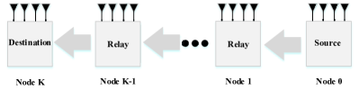
Figure 3: Multi-hop cooperative AF MIMO relaying network.

Based on Lemma 2 in Section II, we have when the rank of $\bm{R}_{{\rm s}_{k}}$ is not higher than the number of columns and the number of rows in ${\bm{F}}_{k}$, the optimal solution ${\bm{F}}_{{\rm opt},k}$ is a square root of $\bm{R}_{{\rm s}_{k}}$.

2) Joint Power Constraints: We have

$$\begin{array}[]{l}\psi_{k,1}\big{(}{\bm{F}}_{k}\big{)}={\rm Tr}\big{(}{\bm{F}}_{k}{\bm{F}}_{k}^{\rm H}\big{)}-P_{k},\\ \psi_{k,2}\big{(}{\bm{F}}_{k}\big{)}={\bm{F}}_{k}{\bm{F}}_{k}^{\rm H}-\tau_{k}\bm{I}.\end{array}$$ (66)

Based on Lemma 2 in Section II, the Pareto optimal solutions $\bm{F}_{{\rm opt},k}$ satisfy the following structure

$$\bm{F}_{{\rm opt},k}=\bm{V}_{\bm{H}_{k}}\bm{\Lambda}_{{\bm{F}}_{k}}\bm{U}_{{\text{Arb}},k}^{\rm H},$$ (67)

where every diagonal element of the rectangular diagonal matrix $\bm{\Lambda}_{\breve{\bm{F}}_{k}}$ is smaller than $\sqrt{\tau_{k}}$. The diagonal matrix $\bm{\Lambda}_{\breve{\bm{F}}_{k}}$ can be efficiently solved using a variant water-filling algorithm [54, 52].

3) Multiple Weighted Power Constraints: We have

$$\psi_{k,i}\big{(}{\bm{F}}_{k}\big{)}={\rm Tr}\big{(}\bm{\Omega}_{k,i}{\bm{F}}_{k}{\bm{F}}_{k}^{\rm H}\big{)}-P_{k,i}.$$ (68)

Based on Lemma 3 in Section II, the Pareto optimal solutions $\bm{F}_{{\rm opt},k}$ satisfy the following structure

$$\bm{F}_{{\rm opt},k}=\bm{\Omega}_{k}^{-\frac{1}{2}}\breve{\bm{V}}_{\bm{\mathcal{H}}_{k}}\bm{\Lambda}_{\breve{\bm{F}}_{k}}{\bm{U}}_{{\rm{Arb}},k}^{\rm H},$$ (69)

where $\bm{\Omega}_{k}$ is given by (51), while $\breve{\bm{V}}_{\bm{\mathcal{H}}_{k}}$ is defined by the following SVD, respectively,

$$\bm{R}_{\bm{n}_{k}}^{-\frac{1}{2}}\bm{H}_{k}\bm{\Omega}_{k}^{-\frac{1}{2}}\!=\!\breve{\bm{U}}_{\bm{\mathcal{H}}_{k}}\breve{\bm{\Lambda}}_{\bm{\mathcal{H}}_{k}}\breve{\bm{V}}_{\bm{\mathcal{H}}_{k}}^{\rm H}\text{ with }\breve{\bm{\Lambda}}_{\bm{\mathcal{H}}_{k}}\searrow.$$ (70)

The diagonal matrix $\bm{\Lambda}_{\breve{\bm{F}}_{k}}$ can be efficiently solved using water-filling algorithms [53, 54].

Remark 1

The results of this paper can also be applied to more complex scenarios. For example, when the CSI between a sensor and its data fusion center is imperfect, $\bm{H}_{k}=\widehat{\bm{H}}_{k}+\bm{H}_{{\rm W},k}\bm{\Psi}_{k}^{\frac{1}{2}}$, where $\widehat{\bm{H}}_{k}$ and $\bm{H}_{{\rm W},k}\bm{\Psi}_{k}^{\frac{1}{2}}$ are the estimated CSI and the channel estimation error, respectively. The correlation matrix $\bm{\Psi}_{k}$ is a function of both the channel estimator and of the training sequence. Based on the proposed framework, the optimal structures of the optimal solutions for the robust signal compression matrices at different sensors can also be readily derived.

V Multi-Hop AF MIMO Relaying Networks

Multi-hop relaying communication is one of the most important enabling technologies for future flexible and high-throughput communications, such as machine-to-machine, device-to-device, vehicle-to-vehicle, internet of things or satellite communications [28, 48]. The key idea behind multi-hop communications is to deploy multiple relays to realize the communications between the source node and destination node [48, 49]. Before presenting our third application of transceiver optimization for multi-hop communications, we first highlight the difference between our work presented in this section and the previous conclusions in [28, 31].

• We consider a more general power constraint which includes both the per-antenna power constraint in [31] and the shaping constraints in [28] as its special cases.

• The channel estimation errors are realistically taken into account in our work. By contrast, in [31] the CSI is assumed to be perfectly known.

To the best of our knowledge, the robust transceiver optimization for multi-hop communications even under the per-antenna power constraint is still the problem not yet fully solved in the existing literature. Therefore, the results presented in this section is novel and significant.

TABLE I: The objective functions and the associated optimal first unitary matrices $\bm{Q}_{1}$ for multi-hop cooperative AF relay networks.

Index	Objective function	Optimal $\bm{Q}_{\bm{X}_{1}}$
Obj. 1	$\log\big{|}\bm{\Phi}_{\rm MSE}\big{(}\{\bm{F}_{k}\}_{k=1}^{K},\{\bm{Q}_{\bm{X}_{k}}\}_{k=1}^{K},\bm{C}=\bm{I}\big{)}|$	$\bm{Q}_{{\rm opt},\bm{X}_{1}}=\bm{V}_{\bm{A}_{1}}\bm{U}_{\rm{Arb}}^{\rm H}$
Obj. 2	${\rm{Tr}}\big{(}\bm{W}\bm{\Phi}_{\rm MSE}\big{(}\{\bm{F}_{k}\}_{k=1}^{K},\{\bm{Q}_{\bm{X}_{k}}\}_{k=1}^{K},\bm{C}=\bm{I}\big{)}\big{)}$	$\bm{Q}_{{\rm opt},\bm{X}_{1}}=\bm{V}_{\bm{A}_{1}}\bm{U}_{\bm{W}}^{\rm H}$
Obj. 3	$f_{\text{A-Schur}}^{\text{Convex}}\big{(}\bm{d}\big{[}\bm{\Phi}_{\rm MSE}\big{(}\{\bm{F}_{k}\}_{k=1}^{K},\{\bm{Q}_{\bm{X}_{k}}\}_{k=1}^{K},\bm{C}=\bm{I}\big{)}\big{]}\big{)}$	$\bm{Q}_{{\rm opt},\bm{X}_{1}}=\bm{V}_{\bm{A}_{1}}\bm{U}_{\rm DFT}^{\rm H}$
Obj. 4	$f_{\text{A-Schur}}^{\text{Concave}}\big{(}\bm{d}\big{[}\bm{\Phi}_{\rm MSE}\big{(}\{\bm{F}_{k}\}_{k=1}^{K},\{\bm{Q}_{\bm{X}_{k}}\}_{k=1}^{K},\bm{C}=\bm{I}\big{)}\big{]}\big{)}$	$\bm{Q}_{{\rm opt},\bm{X}_{1}}=\bm{V}_{\bm{A}_{1}}$
Obj. 5	$f_{\text{M-Schur}}^{\text{Convex}}\big{(}\bm{d}\big{[}\bm{\Phi}_{\rm MSE}\big{(}\{\bm{F}_{k}\}_{k=1}^{K},\{\bm{Q}_{\bm{X}_{k}}\}_{k=1}^{K},\bm{C}\big{)}\big{]}\big{)}$	$\bm{Q}_{{\rm opt},\bm{X}_{1}}=\bm{V}_{\bm{A}_{1}}\widetilde{\bm{U}}_{\rm GMD}^{\rm H}$
Obj. 6	$f_{\text{M-Schur}}^{\text{Concave}}\big{(}\bm{d}\big{[}\bm{\Phi}_{\rm MSE}\big{(}\{\bm{F}_{k}\}_{k=1}^{K},\{\bm{Q}_{\bm{X}_{k}}\}_{k=1}^{K},\bm{C}\big{)}\big{]}\big{)}$	$\bm{Q}_{{\rm opt},\bm{X}_{1}}=\bm{V}_{\bm{A}_{1}}$

The $K$-hop AF MIMO relaying network is illustrated in Fig. 3, where the source, denoted as node 0, communicates with the destination, represented by node $K$, with the help of the $(K-1)$ relays, which are nodes 1 to $(K-1)$. Denote the signal sent by the source as $\bm{x}_{0}$, which has the covariance matrix of $\sigma_{\bm{x}_{0}}^{2}\bm{I}$. Then the signal model in the $k$th hop, for $1\leq k\leq K$, can be expressed as

$$\bm{x}_{k}= \bm{H}_{k}\bm{X}_{k}\bm{x}_{k-1}+\bm{n}_{k},$$ (71)

where $\bm{x}_{k}$ is the signal received by node $k$, $\bm{H}_{k}$ is the channel matrix of the $k$th hop, and $\bm{n}_{k}$ is the additive noise of the corresponding link with the covariance matrix $\sigma_{\bm{n}_{k}}^{2}\bm{I}$, while $\bm{X}_{k}$ is the forwarding matrix of node $(k-1)$. Note that $\bm{S}_{1}$ is the source’s transmit precoding matrix. When the channel estimation error is considered, based on a practical channel estimation scheme [15] the CSI of the $k$th hop is expressed as

$$\bm{H}_{k}= \widehat{\bm{H}}_{k}+\bm{H}_{{\rm W},k}\bm{\Psi}_{k}^{\frac{1}{2}},$$ (72)

where $\widehat{\bm{H}}_{k}$ and $\bm{H}_{{\rm W},k}\bm{\Psi}_{k}^{\frac{1}{2}}$ are the estimated CSI and the channel estimation error of the $k$th hop, respectively. Furthermore, $\bm{\Psi}_{k}$ is the covariance matrix of the channel estimate, and the elements of $\bm{H}_{{\rm W},k}$ follow the independent and identical complex Gaussian distribution $\mathcal{CN}(0,1)$. For notational convenience, let us define the new variables $\bm{F}_{1}\bm{Q}_{\bm{X}_{1}}=\bm{X}_{1}$, with the associated unitary matrix $\bm{Q}_{\bm{X}_{1}}$, and $\bm{F}_{k}\bm{Q}_{k}$ for $2\leq k\leq K$ as

$$\bm{F}_{k}= \bm{X}_{k}\bm{K}_{{\rm{n}}_{k-1}}^{\frac{1}{2}}\bm{M}_{k-1}\bm{Q}_{\bm{X}_{k}}^{\rm H},$$ (73)

where $\bm{Q}_{k}$ is the associated unitary matrix,

$$\bm{M}_{k}\!= \Big{(}\!\bm{K}_{{\rm{n}}_{k}}^{-\frac{1}{2}}\widehat{\bm{H}}_{k}\bm{F}_{k}\bm{F}_{k}^{\rm H}\widehat{\bm{H}}_{k}^{\rm H}\bm{K}_{{\rm{n}}_{k}}^{-\frac{1}{2}}\!+\!\bm{I}\Big{)}^{\frac{1}{2}}\!,\!$$ (74)

$$\bm{K}_{{\rm{n}}_{k}}\!= \Big{(}\sigma_{\rm{n}_{k}}^{2}+{\rm{Tr}}\big{(}\bm{F}_{k}\bm{F}_{k}^{\rm H}\bm{\Psi}_{k}\big{)}\Big{)}\bm{I},$$ (75)

and clearly $\bm{K}_{\rm{n}_{0}}^{\frac{1}{2}}\bm{M}_{0}=\sigma_{\bm{x}_{0}}\bm{I}$. Based on these definitions, as proved in Appendix B the MSE matrix of the data detection at the destination is expressed as, [28, 31]

$$\bm{\Phi}_{\rm MSE}\big{(}\{\bm{F}_{k}\}_{k=1}^{K},\{\bm{Q}_{\bm{X}_{k}}\}_{k=1}^{K},\bm{C}\big{)}$$

$$\hskip 14.22636pt=\sigma_{\bm{x}_{0}}^{2}\bm{C}\bm{C}^{\rm H}-\sigma_{\bm{x}_{0}}^{2}\bm{C}\left(\prod_{k=1}^{K}\bm{M}_{k}^{-\frac{1}{2}}\bm{K}_{{\rm{n}}_{k}}^{-\frac{1}{2}}\widehat{\bm{H}}_{k}\bm{F}_{k}\bm{Q}_{\bm{X}_{k}}\right)^{\rm H}$$

$$\ \ \ \ \ \ \ \ \ \ \ \ \ \times\left(\prod_{k=1}^{K}\bm{M}_{k}^{-\frac{1}{2}}\bm{K}_{\rm{n}_{k}}^{-\frac{1}{2}}\widehat{\bm{H}}_{k}\bm{F}_{k}\bm{Q}_{\bm{X}_{k}}\right)\bm{C}^{\rm H}.$$ (76)

Based on the MSE matrix given in (V), both the linear and nonlinear transceiver optimization problems [28, 31] can be unified into the general optimization problem Opt. 4.1 given in (78). Various objective functions typically adopted for Opt. 4.1 are listed in Table I. For linear transceiver optimization, to realize different levels of fairness between different transmitted data streams, a general objective function can be formulated as an additively Schur-convex function [51, 31] or additively Schur-concave function [51, 31] of the diagonal elements of the MSE matrix, which are given by Obj. 3 and Obj. 4 [51, 31], respectively. The additively Schur-convex function $f_{\text{A-Schur}}^{\rm convex}(\cdot)$ and the additively Schur-concave function $f_{\text{A-Schur}}^{\rm concave}(\cdot)$ represent different levels of fairness among the diagonal elements of the data MSE matrix. When nonlinear transceivers are adopted for improving the BER performance at the cost of increased complexity, e.g., THP or DFE, the objective functions of the transceiver optimization can be formulated as a multiplicative Schur-convex function or a multiplicative Schur-concave function of the vector consisting of the squared diagonal elements of the Cholesky-decomposition triangular matrix of the MSE matrix, that is, Obj. 5 and Obj. 6 [51, 31], respectively, where $\bm{L}$ is a lower triangular matrix. The multiplicatively Schur-convex function $f_{\text{M-Schur}}^{\rm convex}(\cdot)$ and the multiplicatively Schur-concave function $f_{\text{M-Schur}}^{\rm concave}(\cdot)$ reflect the different levels of fairness among the different data streams, i.e., different tradeoffs among the performance of different data steams [17]. The detailed definitions of $f_{\text{A-Schur}}^{\rm convex}(\cdot)$, $f_{\text{A-Schur}}^{\rm concave}(\cdot)$, $f_{\text{M-Schur}}^{\rm convex}(\cdot)$ and $f_{\text{M-Schur}}^{\rm concave}(\cdot)$ are given in Appendix C. This appendix makes our work self-contained.

The constraints $\psi_{k,i}(\bm{F}_{k})\leq 0$ are right unitarily invariant, and the power constraint model of Opt. 4.1 is more general than the power constraint models considered in [17, 28, 31].

For linear transceivers with the objective functions Objs. 1-4 in Table I, $\bm{C}=\bm{I}$ is an identity matrix, while for nonlinear transceiver optimization with the objective functions Obj. 5 and Obj. 6 in Table I , $\bm{C}$ is a lower triangular matrix. Specifically, we assume that the size of $\bm{C}$ is $N\times N$. Then, for nonlinear transceivers, the optimal $\bm{C}$ satisfies [31]

$$\bm{C}_{\rm opt}= {\rm diag}\big{\{}\{[\bm{L}]_{i,i}\}_{i=1}^{N}\big{\}}\bm{L}^{-1},$$ (76)

where $\bm{L}$ is the triangular matrix of the Cholesky decomposition of the following matrix [31]

$$\bm{L}\bm{L}^{\rm H}= \widetilde{\bm{\Phi}}_{\rm MSE}\big{(}\{\bm{F}_{k}\}_{k=1}^{K},\{\bm{Q}_{\bm{X}_{k}}\}_{k=1}^{K}\big{)}$$

$$= \sigma_{\bm{x}_{0}}^{2}\bm{I}-\sigma_{\bm{x}_{0}}^{2}\left(\prod_{k=1}^{K}\bm{M}_{k}^{-\frac{1}{2}}\bm{K}_{{\rm{n}}_{k}}^{-\frac{1}{2}}\widehat{\bm{H}}_{k}\bm{F}_{k}\bm{Q}_{\bm{X}_{k}}\right)^{\rm H}$$

$$\hskip 28.45274pt\times\left(\prod_{k=1}^{K}\bm{M}_{k}^{-\frac{1}{2}}\bm{K}_{{\rm{n}}_{k}}^{-\frac{1}{2}}\widehat{\bm{H}}_{k}\bm{F}_{k}\bm{Q}_{\bm{X}_{k}}\right).$$ (77)

The optimal unitary matrices $\bm{Q}_{\bm{X}_{k}}$ can be derived based on majorization theory. Specifically, the optimal $\bm{Q}_{k}$ for $k>1$ are derived as [28, 31, 26]

$$\bm{Q}_{{\rm opt},\bm{X}_{k}}= \bm{V}_{\bm{A}_{k}}\bm{U}_{\bm{A}_{k-1}}^{\rm H},$$ (78)

where the unitary matrices $\bm{V}_{\bm{A}_{k}}$ and $\bm{U}_{\bm{A}_{k}}$ are defined by the following SVDs

$$\bm{M}_{k}^{-\frac{1}{2}}\bm{K}_{{\rm{n}}_{k}}^{-\frac{1}{2}}\widehat{\bm{H}}_{k}\bm{F}_{k}= \bm{U}_{\bm{A}_{k}}\bm{\Lambda}_{\bm{A}_{k}}\bm{V}_{\bm{A}_{k}}^{\rm H}\text{ with }\bm{\Lambda}_{\bm{A}_{k}}\searrow.$$ (79)

The optimal $\bm{Q}_{\bm{X}_{1}}$ is determined by the specific objective function, and various $\bm{Q}_{{\rm opt},\bm{X}_{1}}$ associated with different objective functions are also summarized in Table I. Here, the unitary matrix $\bm{U}_{\rm{Arb}}$ denotes an arbitrary matrix having the appropriate dimension. The unitary matrix $\bm{U}_{\bm{W}}$ is the unitary matrix defined by the following EVD

$$\bm{W}= \bm{U}_{\bm{W}}\bm{\Lambda}_{\bm{W}}\bm{U}_{\bm{W}}^{\rm H}\text{ with }\bm{\Lambda}_{\bm{W}}\searrow.$$ (80)

The unitary matrix $\bm{U}_{\rm DFT}$ is a DFT matrix [55, 56]. Finally, the unitary matrix $\widetilde{\bm{U}}_{\rm GMD}$ ensures that the triangular matrix of the Cholesky decomposition of $\widetilde{\bm{\Phi}}_{\rm MSE}\big{(}\{\bm{F}_{k}\}_{k=1}^{K},\{\bm{Q}_{\bm{X}_{k}}\}_{k=1}^{K}\big{)}$ has the same diagonal elements [31].

Given the optimal $\bm{Q}_{{\rm opt},\bm{X}_{k}}$ and $\bm{C}_{\rm opt}$, the objective function of Opt. 4.1 can be rewritten as [28]

$$f\left(\bm{\Phi}_{\rm MSE}\big{(}\{\bm{F}_{k}\}_{k=1}^{K},\{\bm{Q}_{{\rm opt},\bm{X}_{k}}\}_{k=1}^{K},\bm{C}_{\rm opt}\big{)}\right)$$

$$= \widetilde{f}\left(\left\{\prod_{k=1}^{K}\frac{\lambda_{i}(\bm{F}_{k}^{\rm H}\widehat{\bm{H}}_{k}^{\rm H}\bm{K}_{{\rm{n}}_{k}}^{-1}\widehat{\bm{H}}_{k}\bm{F}_{k})}{1+\lambda_{i}(\bm{F}^{\rm H}_{k}\widehat{\bm{H}}_{k}^{\rm H}\bm{K}_{{\rm{n}}_{k}}^{-1}\widehat{\bm{H}}_{k}\bm{F}_{k})}\right\}_{i=1}^{N}\right)$$

$$\triangleq f_{\text{Eigen}}\left(\left\{\bm{\lambda}\big{(}\bm{F}_{k}^{\rm H}\widehat{\bm{H}}_{k}^{\rm H}\bm{K}_{{\rm{n}}_{k}}^{-1}\widehat{\bm{H}}_{k}\bm{F}_{k}\big{)}\right\}_{k=1}^{K}\right).$$ (81)

In (V) $f_{\text{Eigen}}(\cdot)$ is a monotonically decreasing function with respect to the eigenvalue vector $\bm{\lambda}\big{(}\bm{F}_{k}^{\rm H}\widehat{\bm{H}}_{k}^{\rm H}\bm{K}_{{\rm{n}}_{k}}^{-1}\widehat{\bm{H}}_{k}\bm{F}_{k}\big{)}$. The specific formula of $f_{\text{Eigen}}(\cdot)$ is determined by the specific performance metrics. For example, for sum MSE minimization $f_{\text{Eigen}}(\cdot)$ equals

$$f_{\text{Eigen}}\left(\left\{\bm{\lambda}\big{(}\bm{F}_{k}^{\rm H}\widehat{\bm{H}}_{k}^{\rm H}\bm{K}_{{\rm{n}}_{k}}^{-1}\widehat{\bm{H}}_{k}\bm{F}_{k}\big{)}\right\}_{k=1}^{K}\right)$$

$$= \sum_{i=1}^{I}x_{0}^{2}\left(1-\prod_{k=1}^{K}\frac{\lambda_{i}(\bm{F}_{k}^{\rm H}\widehat{\bm{H}}_{k}^{\rm H}\bm{K}_{\rm{n}_{k}}^{-1}\widehat{\bm{H}}_{k}\bm{F}_{k})}{1+\lambda_{i}(\bm{F}^{\rm H}_{k}\widehat{\bm{H}}_{k}^{\rm H}\bm{K}_{{\rm{n}}_{k}}^{-1}\widehat{\bm{H}}_{k}\bm{F}_{k})}\right).$$ (82)

In addition, for sum rate maximization $f_{\text{Eigen}}(\cdot)$ equals

$$f_{\text{Eigen}}\left(\left\{\bm{\lambda}\big{(}\bm{F}_{k}^{\rm H}\widehat{\bm{H}}_{k}^{\rm H}\bm{K}_{{\rm{n}}_{k}}^{-1}\widehat{\bm{H}}_{k}\bm{F}_{k}\big{)}\right\}_{k=1}^{K}\right)$$

$$= \sum_{i=1}^{I}{\rm{log}}\left(1-\prod_{k=1}^{K}\frac{\lambda_{i}(\bm{F}_{k}^{\rm H}\widehat{\bm{H}}_{k}^{\rm H}\bm{K}_{\rm{n}_{k}}^{-1}\widehat{\bm{H}}_{k}\bm{F}_{k})}{1+\lambda_{i}(\bm{F}^{\rm H}_{k}\widehat{\bm{H}}_{k}^{\rm H}\bm{K}_{{\rm{n}}_{k}}^{-1}\widehat{\bm{H}}_{k}\bm{F}_{k})}\right).$$ (83)

Hence, given $\bm{Q}_{{\rm opt},\bm{X}_{k}}$ and $\bm{C}_{\rm opt}$, Opt. 4.1 is transferred into

$$\begin{array}[]{lcl}\textbf{Opt.\,4.2:}\!\!&\!\!\min\limits_{\{\bm{F}_{k}\}_{k=1}^{K}}\!\!&\!\!f_{\text{Eigen}}\left(\left\{\bm{\lambda}\big{(}\bm{F}_{k}^{\rm H}\widehat{\bm{H}}_{k}^{\rm H}\bm{K}_{\rm{n}_{k}}^{-1}\widehat{\bm{H}}_{k}\bm{F}_{k}\big{)}\right\}_{k=1}^{K}\right)\!,\\ \!\!&\!\!{\rm{s.t.}}\!\!&\!\!\bm{K}_{\rm{n}_{k}}=\Big{(}\sigma_{\rm{n}_{k}}^{2}+{\rm{Tr}}\big{(}\bm{F}_{k}\bm{F}_{k}^{\rm H}\bm{\Psi}_{k}\big{)}\Big{)}\bm{I},\\ \!\!&\!\!\!\!&\!\!\psi_{k,i}(\bm{F}_{k})\leq 0,1\leq i\leq I_{k},1\leq k\leq K.\end{array}$$ (87)

Since the objective function of Opt. 4.2 is a monotonically decreasing function of $\bm{\lambda}\big{(}\bm{F}_{k}^{\rm H}\widehat{\bm{H}}_{k}^{\rm H}\bm{K}_{{\rm{n}}_{k}}^{-1}\widehat{\bm{H}}_{k}\bm{F}_{k}\big{)}$, it can be decoupled into the following sub-problems: for $1\leq k\leq K$,

$$\begin{array}[]{lcl}\textbf{Opt.\,4.3:}&\min\limits_{\bm{F}_{k}}&\bm{\lambda}\big{(}\bm{F}_{k}^{\rm H}\widehat{\bm{H}}_{k}^{\rm H}\bm{K}_{\rm{n}_{k}}^{-1}\widehat{\bm{H}}_{k}\bm{F}_{k}\big{)},\\ &{\rm{s.t.}}&\bm{K}_{\rm{n}_{k}}=\Big{(}\sigma_{\rm{n}_{k}}^{2}\!+\!{\rm{Tr}}\big{(}\bm{F}_{k}\bm{F}_{k}^{\rm H}\bm{\Psi}_{k}\big{)}\Big{)}\bm{I},\\ &&\psi_{k,i}(\bm{F}_{k})\leq 0,1\leq i\leq I_{k}.\end{array}$$ (91)

Clearly, Opt. 4.3 is equivalent to the following matrix-monotonic optimization problem

$$\begin{array}[]{lcl}\textbf{Opt.\,4.4:}&\min\limits_{\bm{F}_{k}}&\bm{F}_{k}^{\rm H}\widehat{\bm{H}}_{k}^{\rm H}\bm{K}_{\rm{n}_{k}}^{-1}\widehat{\bm{H}}_{k}\bm{F}_{k},\\ &{\rm{s.t.}}&\bm{K}_{\rm{n}_{k}}=\Big{(}\sigma_{\rm{n}_{k}}^{2}\!+\!{\rm{Tr}}\big{(}\bm{F}_{k}\bm{F}_{k}^{\rm H}\bm{\Psi}_{k}\big{)}\Big{)}\bm{I},\\ &&\psi_{k,i}(\bm{F}_{k})\leq 0,1\leq i\leq I_{k}.\end{array}$$ (95)

In this application, by exploiting its cascade structure, we are able to transfer the associated multiple-matrix-variate matrix-monotonic optimization problem into several single-matrix-variate matrix-monotonic optimization problems. Based on the fundamental results of the previous sections, we readily have the following results.

1) Shaping Constraint: We have $I_{k}=1$ and

$$\psi_{k,1}(\bm{F}_{k})= \bm{F}_{k}\bm{F}_{k}^{\rm H}-\bm{R}_{{\rm s}_{k}}.$$ (96)

As proved in Part I, based on Lemma 1 in Section II, it is concluded that when the rank of $\bm{R}_{{\rm s}_{k}}$ is not higher than the number of columns and the number of rows in $\bm{F}_{k}$, a suboptimal solution $\bm{F}_{{\rm opt},k}$ that maximizes a lower bound of the objective of Opt. 4.4 is a square root of $\bm{R}_{{\rm s}_{k}}$. When $\bm{\Psi}_{k}=\bm{0}$ the lower bound is tight and then the suboptimal solution will be the Pareto optimal solution of Opt. 4.4.

2) Joint Power Constraint: We have

$$\begin{array}[]{l}\psi_{k,1}\big{(}{\bm{F}}_{k}\big{)}={\rm Tr}\big{(}{\bm{F}}_{k}{\bm{F}}_{k}^{\rm H}\big{)}-P_{k},\\ \psi_{k,2}\big{(}{\bm{F}}_{k}\big{)}={\bm{F}}_{k}{\bm{F}}_{k}^{\rm H}-\tau_{k}\bm{I}.\end{array}$$ (99)

As proved in Part I, based on Lemma 2 in in Section II for the general case $\bm{\Psi}_{k}\not\propto\bm{I}$, a suboptimal solution that maximizes a lower bound of the objective of Opt. 4.4 satisfies the following structure

$$\bm{F}_{k}=\frac{\sigma_{{\rm{n}}_{k}}\widetilde{\bm{\Psi}}_{k}^{-\frac{1}{2}}{\bm{V}}_{\widetilde{\bm{H}}_{k}}\bm{\Lambda}_{\widetilde{\bm{F}}_{k}}{\bm{U}}_{{\rm{Arb}},k}^{\rm{H}}}{\left(1-{\rm{Tr}}\left(\widetilde{\bm{\Psi}}_{k}^{-\frac{1}{2}}\bm{\Psi}\widetilde{\bm{\Psi}}_{k}^{-\frac{1}{2}}{\bm{V}}_{\widetilde{\bm{H}}_{k}}\bm{\Lambda}_{\widetilde{\bm{F}}_{k}}\bm{\Lambda}_{\widetilde{\bm{F}}_{k}}^{\rm{H}}{\bm{V}}_{\widetilde{\bm{H}}_{k}}^{\rm{H}}\right)\right)^{\frac{1}{2}}},$$ (100)

where $\widetilde{\bm{\Psi}}_{k}=\sigma_{{\rm{n}}_{k}}^{2}\bm{I}+P_{k}\bm{\Psi}_{k}$. It is worth noting that when $\bm{\Psi}_{k}=\bm{0}$ or $\bm{\Psi}_{k}\propto\bm{I}$, the corresponding lower bound is tight. In other words, in that case the suboptimal solution is exactly the Pareto optimal solution of Opt. 4.4. The unitary matrix $\bm{V}_{\widetilde{\bm{H}}_{k}}$ is the right unitary matrix of the following SVD

$$\widehat{\bm{H}}_{k}\big{(}\sigma_{{\rm{n}}_{k}}^{2}\bm{I}+P_{k}\bm{\Psi}_{k}\big{)}^{-\frac{1}{2}}={\bm{U}}_{\widetilde{\bm{H}}_{k}}\bm{\Lambda}_{\widetilde{\bm{H}}_{k}}{\bm{V}}_{\widetilde{\bm{H}}_{k}}^{H},\text{with}\ \bm{\Lambda}_{\widetilde{\bm{H}}_{k}}\searrow,$$ (101)

and every diagonal element of the rectangular diagonal matrix ${{\bm{\Lambda}}}_{\widetilde{\bm{F}}_{k}}$ in (100) is smaller than the following threshold

$$\sqrt{\tau_{k}\big{(}\sigma_{{\rm{n}}_{k}}^{2}+P_{k}\lambda_{\min}(\bm{\Psi}_{k})\big{)}/\big{(}\sigma_{{\rm{n}}_{k}}^{2}+P_{k}\lambda_{\max}(\bm{\Psi}_{k})\big{)}}.$$ (102)

The diagonal matrix $\bm{\Lambda}_{\widetilde{\bm{F}}_{k}}$ can be efficiently solved using a variant water-filling algorithm [54, 53].

3) Multiple weighted power constraints: We have

$$\psi_{k,i}\big{(}{\bm{F}}_{k}\big{)}= {\rm Tr}\big{(}\bm{\Omega}_{k,i}{\bm{F}}_{k}{\bm{F}}_{k}^{\rm H}\big{)}-P_{k,i}.$$ (103)

As proved in Part I, based on Lemma 3 in Section II, we conclude that the Pareto optimal solutions $\bm{F}_{{\rm opt},k}$ satisfy the following structure

$$\bm{F}_{{\rm opt},k}\!= \frac{\sigma_{{\rm{n}}_{k}}\widetilde{\bm{\Omega}}_{k}^{-\frac{1}{2}}\bm{V}_{\bm{\mathcal{H}}_{k}}\bm{\Lambda}_{\widetilde{\bm{F}}_{k}}\bm{U}_{\text{Arb},k}^{\rm H}}{\Big{(}\!1\!-\!{\rm{Tr}}\big{(}\widetilde{\bm{\Omega}}_{k}^{-\frac{1}{2}}\bm{\Psi}_{k}\widetilde{\bm{\Omega}}_{k}^{-\frac{1}{2}}\bm{V}_{\bm{\mathcal{H}}_{k}}\bm{\Lambda}_{\widetilde{\bm{F}}_{k}}\bm{\Lambda}_{\widetilde{\bm{F}}_{k}}^{\rm H}\bm{V}_{\bm{\mathcal{H}}_{k}}^{\rm H}\big{)}\!\Big{)}^{\frac{1}{2}}},\!$$ (104)

where the unitary matrix $\bm{V}_{\bm{\mathcal{H}}_{k}}$ is defined by the SVD

$$\widehat{\bm{H}}_{k}\widetilde{\bm{\Omega}}_{k}^{-\frac{1}{2}}= \bm{U}_{\bm{\mathcal{H}}_{k}}\bm{\Lambda}_{\bm{\mathcal{H}}_{k}}\bm{V}_{\bm{\mathcal{H}}_{k}}^{\rm H}\text{ with }\bm{\Lambda}_{\bm{\mathcal{H}}_{k}}\searrow,$$ (105)

and the matrix $\widetilde{\bm{\Omega}}_{k}$ is defined by

$$\widetilde{\bm{\Omega}}_{k}= \sigma_{\rm{n}_{k}}^{2}\sum\nolimits_{i=1}^{I_{k}}\alpha_{k,i}\big{(}\bm{\Omega}_{k,i}+P_{k,i}\bm{\Psi}_{k}\big{)}.$$ (106)

The diagonal matrix $\bm{\Lambda}_{\widetilde{\bm{F}}_{k}}$ can be efficiently solved using water-filling algorithms [53, 54].

VI Discussions

In this paper, we have investigated three representative examples for the proposed framework of multi-variable matrix-monotonic optimization. Based on the proposed matrix-monotonic framework, the structure of the optimal solutions for the three largely different optimization problems can be derived in the same logic. The distinct difference between our work and existing work is that more general power constraints have been taken in account. Taking more general power constraints into account is definitely not trivial extensions. From physical meaning perspective, the considered optimization under more general power constraints includes more MIMO transceiver optimizations as its special cases. Moreover, from a mathematical viewpoint, the optimization with more general power constraints is more challenging. It is impossible to extend the existing results in the literature to the conclusions given in this paper via using simple substitutions. From convex optimization theory perspective, adding one more constraint may not change the convexity of the considered optimization problem. Specifically, adding one more linear matrix inequality on a SDP problem, the resulting problem is still a SDP problem. Adding a quadratical constraint on a QCQP problem, the resulting problem is still a QCQP. The story is totally different for the matrix-monotonic optimization framework as the matrix-monotonic optimization framework aims at deriving the structure of the optimal solutions. One more constraint will change the feasible region of matrix variate and significantly change the structure of the optimal solutions. The corresponding analytical derivations will change distinctly.

We also would like to point out that the matrix-monotonic optimization framework is applicable to more complicated communication systems. Recently, in [18] based on the matrix-monotonic optimization framework, a general framework on hybrid transceiver optimizations under sum power constraint is proposed. Different from the fully digital MIMO systems, in a typical hybrid MIMO system, at the source or the destination the precoder or the receiver consists of two parts, i.e., analog part and digital part. For the analog part, only the phase of the signal at each antenna is adjustable. After that, in [19] based on the matrix-monotonic optimization framework, a framework on the transceiver optimizations for multi-hop AF hybrid MIMO relaying systems is further proposed. In multi-hop communications, the forwarding matrix at each relay consists of three parts, the left analog part, the inner digital part and the right analog part.

VII Simulation Results and Discussions

VII-A Two-user MIMO Uplink

We first consider the MU-MIMO uplink, where a pair of 4-antenna mobile users communicate with an 8-antenna BS. We define $\frac{P_{k}}{\sigma_{n}^{2}}$ as the SNR for the $k$th user, where $P_{k}$ is the sum transmit power of user $k$ and $\sigma_{n}^{2}$ is the noise power at each receive antenna of the BS. Without loss of generality, the same maximum transmit power is assumed for all the users, i.e., $P_{1}=P_{2}$. Based on the Kronecker correlation model [15, 13, 14], the spatial correlation matrix $\bm{R}_{\rm Rx}$ of the BS’s receive antennas and the spatial correlation matrix $\bm{R}_{{\rm Tx},k}$ of the $k$th user’s transmit antennas, where $k=1,2$, are specified respectively by $\big{[}\bm{R}_{\rm Rx}\big{]}_{i,j}=r_{\rm r}^{|i-j|}$ and $\big{[}\bm{R}_{{\rm Tx},k}\big{]}_{i,j}=r_{{\rm t},k}^{|i-j|}$. In the simulations, we further set $r_{{\rm t},1}=r_{{\rm t},2}=r_{{\rm t}}$. Three power constraints, namely, the shaping constraint, the joint power constraint and the per-antenna power constraints, are considered. For the shaping constraint, the widely used Kronecker correlation model of $\big{[}\bm{R}_{{\rm s}_{k}}\big{]}_{i,j}=0.6^{|i-j|}$ is employed [28]. For the joint power constraint, the threshold is chosen as $\tau_{k}=1.4$. For the per-antenna power constraints, the power limits for the four antennas of each user are set to 1.2, 1.2, 0.8 and 0.8, respectively.

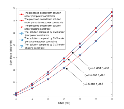
Figure 4: Sum rate performance comparison between the proposed closed-form solutions and the solutions computed by the CVX tool for the two-user MIMO Uplink.

It is worth highlighting that the transceiver optimization under these three power constraints can be transferred into convex optimization problems, which can be solved numerically using the CVX tool [58]. This approach however suffers from high computational complexity, especially for high dimensional antenna arrays. By contrast, our approach presented in Section III provides the optimal closed-form solutions for the same transceiver optimization design problems. Fig. 4 compares the sum rate performance as the function of the SNR for the proposed closed-form solutions and for the numerical optimization solutions computed by the CVX tool. It can be seen that our closed-form solutions have an identical performance to the solutions computed by the CVX tool.

VII-B Signal Compression for Distributed Sensor Networks

In this subsection, we investigate the performance of the proposed algorithm employed for signal compression in distributed sensor networks. Specifically, the distributed sensor network considered consists of $K$ sensors and a data fusion center. Each sensor is equipped with 4 antennas and the data fusion center is equipped with 8 antennas. The per-antenna power constraints for the four antennas of each sensor are set to 1.2, 1.2, 0.8 and $0.8$, respectively. For the signal correlations between different sensors, the distance-dependent correlation matrix model of [27] is adopted. Specifically, we have $\bm{R}_{\bm{x}_{m,n}}=e^{-d_{m,n}}{\bm{I}}$ for the $m$th sensor and the for the $n$th sensor, where $d_{m,n}$ is the correlation between these two sensors. In our simulations, $d_{m,n}$ is distributed uniformly between 0 and 1. In order to quantify the performance advantages attained, a benchmark algorithm based on CVX is used in this subsection. The algorithm based on CVX aims for minimizing the weighted sum MSE under per-antenna power constraints, which is termed as the linear minimum mean square error (LMMSE) algorithm. In the LMMSE algorithm, the signal compression matrices of the different sensors and the combiner matrix at the data fusion center are optimized iteratively. At each iteration, the optimization problem considered is a standard QCQP problem, which can be readily solved by CVX. Observe in Fig. 5 that the proposed algorithm always outperforms the CVX-based benchmarker.

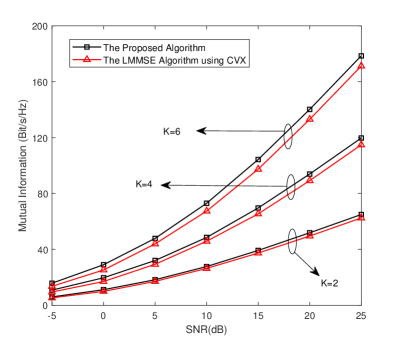
Figure 5: Mutual information performance comparisons between the proposed algorithm and the LMMSE algorithm based on CVX for distributed sensor networks with different numbers of sensors.

VII-C Dual-hop AF MIMO Relaying Network

A dual-hop AF MIMO relaying network is simulated, which consists of one source, one relay and one destination. All the nodes are equipped with 4 antennas. At the source and relay, per-antenna power constraints are imposed. Specifically, the power limits for the four antennas are set as 1, 1, 1 and 1, respectively. The SNR in each hop is defined as the ratio between the transmit power and the noise variance, i.e., $\text{SNR}_{k}=\frac{P_{k}}{\sigma_{{\rm{n}}_{k}}^{2}}$. Without loss of generality, the SNRs in the both hops are assumed to be the same, namely, $\text{SNR}_{1}=\text{SNR}_{2}=\text{SNR}$.

In contrast to the existing works [28, 31], which consider the transceiver optimization unrealistically with the perfect CSI, in this paper, we focus on the robust transceiver optimization, which takes into account the channel estimation error. In the simulations, the estimated channel matrix is generated according to $\widehat{\bm{H}}_{k}=\widehat{\bm{H}}_{{\rm{W}},k}\bm{\Psi}_{k}^{\frac{1}{2}}$ [17], where we have $\big{[}\bm{\Psi}_{k}\big{]}_{i,j}=0.6^{|i-j|}$. The elements of $\widehat{\bm{H}}_{{\rm{W}},k}$ are independently identically distributed Gaussian random variables. In order to ensure that $\mathbb{E}\big{\{}\big{[}\bm{H}\big{]}_{i,j}\big{[}\bm{H}\big{]}_{i,j}^{*}\big{\}}=1$, $\forall i,j$, we set $\mathbb{E}\big{\{}\big{[}\bm{H}_{{\rm W},k}\big{]}_{i,j}\big{[}\bm{H}_{{\rm W},k}\big{]}_{i,j}^{*}\big{\}}=\sigma_{e_{k}}^{2}$ and $\mathbb{E}\big{\{}\big{[}\widehat{\bm{H}}_{{\rm W},k}\big{]}_{i,j}\big{[}\widehat{\bm{H}}_{{\rm W},k}\big{]}_{i,j}^{*}\big{\}}=1-\sigma_{e_{k}}^{2}$. Without loss of generality, we assume $\sigma_{e_{1}}^{2}=\sigma_{e_{2}}^{2}=\sigma_{e}^{2}$. It can be seen from Fig. 6 that our robust design achieves better sum rate performance than the non-robust design of [31]. Furthermore, as expected, the performance gap between the robust and non-robust designs becomes larger as the channel estimation error increases.

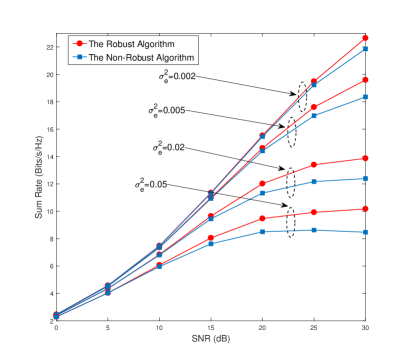
Figure 6: Sum rate performance comparison between our proposed robust design and the non-robust design of [31] for the dual-hop AF MIMO relaying network.

VIII Conclusions

In this paper, we investigated the application of the framework of matrix-monotonic optimization in the optimizations with multiple matrix-variates. It is shown that when several properties are satisfied, the framework of matrix-monotonic optimization still works, based on which the optimal structures of multiple matrix-variates can be derived. Then the multiple matrix-variable optimizations can be effectively solved in iterative manners. Three specific examples are also given in this paper to verify the validity of the proposed multi-variable matrix-monotonic optimization framework. Specifically, under various power constraints, i.e., sum power constraint, shaping constraints, joint power constraints and multiple weighted power constraints, the transceiver optimizations for uplink MIMO communications, the compression matrix optimizations for distributed sensor networks, and the robust transceiver optimizations for multi-hop AF MIMO relaying systems have been investigated. At the end of this paper, several numerical results demonstrated the accuracy and performance advantages of the proposed multi-variable matrix-monotonic optimization framework.

Appendix A Computation of $\bm{P}_{k}$ and $\bm{\Xi}_{k}$

Given the following block diagonal matrix

$$\bm{\Phi}={\rm diag}\Big{\{}\big{\{}\bm{X}_{k}^{\rm H}\bm{H}_{k}^{\rm H}\bm{R}_{\rm{n}_{k}}^{-1}\bm{H}_{k}\bm{X}_{k}\big{\}}_{k=1}^{K}\Big{\}}$$ (107)

the permutation matrix $\bm{P}_{k}$ aims at changing the orders of the $k$th element $\bm{X}_{k}^{\rm H}\bm{H}_{k}^{\rm H}\bm{R}_{\rm{n}_{k}}^{-1}\bm{H}_{k}\bm{X}_{k}$ and the first element $\bm{X}_{1}^{\rm H}\bm{H}_{1}^{\rm H}\bm{R}_{\rm{n}_{1}}^{-1}\bm{H}_{1}\bm{X}_{1}$ along the diagonal line. Before constructing $\bm{P}$, we first give an identity matrix $\bm{I}$ that has the same dimensions as $\bm{\Phi}$. Moreover, $\bm{I}$ can be interpreted as a block diagonal matrix as

$${\bm{I}}={\rm{diag}}\Big{\{}\big{\{}\bm{I}_{k}\big{\}}_{k=1}^{K}\Big{\}}$$ (108)

where $\bm{I}_{k}$ is an identity matrix of the same dimensions as $\bm{X}_{k}^{\rm H}\bm{H}_{k}^{\rm H}\bm{R}_{\rm{n}_{k}}^{-1}\bm{H}_{k}\bm{X}_{k}$ for $1\leq k\leq K$. Moreover, $\bm{I}$ is further divided into the following submatrices

$${\bm{I}}={\rm{diag}}\Big{\{}\big{\{}\bm{I}_{k}\big{\}}_{k=1}^{K}\Big{\}}=\left[{\begin{array}[]{*{20}{c}}{{\bm{\mathcal{I}}}_{1}}\\ {{\bm{\mathcal{I}}}_{2}}\\ {\vdots}\\ {{\bm{\mathcal{I}}}_{K}}\end{array}}\right]$$ (113)

where ${\bm{\mathcal{I}}}_{k}$ and ${\bm{I}}_{k}$ have the same row number for $1\leq k\leq K$. Based on the above definitions of ${\bm{\mathcal{I}}}_{k}$’s, we have

$${\bm{\mathcal{I}}}_{k}\bm{\Phi}{\bm{\mathcal{I}}}_{j}^{\rm{H}}={\bm{\mathcal{I}}}_{k}\bm{\Phi}{\bm{\mathcal{I}}}_{j}^{\rm{T}}={\bm{0}},{\rm{for}},k\not=j,$$ (114)

and

$${\bm{\mathcal{I}}}_{k}\bm{\Phi}{\bm{\mathcal{I}}}_{k}^{\rm{H}}={\bm{\mathcal{I}}}_{k}\bm{\Phi}{\bm{\mathcal{I}}}_{k}^{\rm{T}}=\bm{X}_{k}^{\rm H}\bm{H}_{k}^{\rm H}\bm{R}_{\rm{n}_{k}}^{-1}\bm{H}_{k}\bm{X}_{k}.$$ (115)

Therefore, based on (113) $\bm{P}_{k}$ is constructed by interchanging ${\bm{\mathcal{I}}}_{1}$ and ${\bm{\mathcal{I}}}_{k}$, i.e.,

$$\bm{P}_{k}=\left[{\begin{array}[]{*{20}{c}}{{\bm{\mathcal{I}}}_{k}}\\ {{\bm{\mathcal{I}}}_{2}}\\ {\vdots}\\ {{\bm{\mathcal{I}}}_{k-1}}\\ {{\bm{\mathcal{I}}}_{1}}\\ {{\bm{\mathcal{I}}}_{k+1}}\\ {\vdots}\\ {{\bm{\mathcal{I}}}_{K}}\end{array}}\right].$$ (124)

It is obvious that $\bm{P}_{k}$ is a unitary matrix, i.e.,

$$\bm{P}_{k}\bm{P}_{k}^{\rm{H}}=\bm{I}\ \text{and}\ \bm{P}_{k}^{\rm{H}}\bm{P}_{k}=\bm{I}.$$ (125)

Based on (124) and together with (114) and (115), we have

$$\bm{P}_{k}{\rm diag}\Big{\{}\big{\{}\bm{X}_{k}^{\rm H}\bm{H}_{k}^{\rm H}\bm{R}_{{\rm{n}}_{k}}^{-1}\bm{H}_{k}\bm{X}_{k}\big{\}}_{k=1}^{K}\Big{\}}\bm{P}_{k}^{\rm H}$$

$$= \left[\begin{array}[]{cc}\bm{X}_{k}^{\rm H}\bm{H}_{k}^{\rm H}\bm{R}_{\rm{n}_{k}}^{-1}\bm{H}_{k}\bm{X}_{k}&\bm{0}\\ \bm{0}&\bm{\Xi}_{k}\end{array}\right].$$ (128)

where $\bm{\Xi}_{k}$ is the following block diagonal matrix

$$\bm{\Xi}_{k}={\rm{diag}}\{\widetilde{\bm{\Phi}}_{2},\cdots,\widetilde{\bm{\Phi}}_{k-1},\widetilde{\bm{\Phi}}_{1},\widetilde{\bm{\Phi}}_{k+1},\cdots,\widetilde{\bm{\Phi}}_{K}\}$$ (129)

with $\widetilde{\bm{\Phi}}_{j}=\bm{X}_{j}^{\rm H}\bm{H}_{j}^{\rm H}\bm{R}_{\rm{n}_{j}}^{-1}\bm{H}_{j}\bm{X}_{j}$.

Appendix B MSE Matrix for Multi-Hop Communications

Based on the signal model given in (71), at the destination the received signal $\bm{y}$ equals

$$\bm{y}=\bm{x}_{K}= \bm{H}_{K}\bm{X}_{K}\bm{x}_{K-1}+\bm{n}_{K}.$$ (130)

After performing a linear equalizer $\bm{G}$, the signal estimation MSE matrix at the destination can be written in the following formula [26, 31, 28]

$$\bm{\Phi}_{\rm MSE}\big{(}\bm{G},\{\bm{X}_{k}\}_{k=1}^{K},\bm{C}\big{)}$$

$$=\mathbb{E}\{({\bm{G}}{\bm{y}}-\bm{C}\bm{x}_{0})({\bm{G}}{\bm{y}}-\bm{C}\bm{x}_{0})^{\rm{H}}\}$$ (131)

where $\bm{C}=\bm{I}+\bm{B}$ and $\bm{B}$ is a strictly lower triangular matrix [17]. For the linear transceivers, $\bm{B}$ is a constant matrix, i.e., $\bm{B}=\bm{0}$. On the other hand for the nonlinear transceivers with THP or DFE, $\bm{B}$ corresponds to the feedback operations and should be optimized as well [26, 31, 28]. Substituting (130) into $\bm{\Phi}_{\rm MSE}\big{(}\bm{G},\{\bm{X}_{k}\}_{k=1}^{K}\big{)}$ in (B), we have

$$\bm{\Phi}_{\rm MSE}\big{(}\bm{G},\{\bm{X}_{k}\}_{k=1}^{K},\bm{C}\big{)}$$

$$= \bm{G}\left(\bm{\widehat{H}}_{K}\bm{X}_{K}\bm{R}_{\bm{x}_{K-1}}\bm{X}_{K}^{\rm{H}}\bm{\widehat{H}}_{K}^{\rm{H}}+{\rm{Tr}}(\bm{X}_{K}\bm{R}_{\bm{x}_{K-1}}\bm{X}_{K}^{\rm{H}}{\bm{\Psi}}_{K})\bm{I}\right)\bm{G}^{\rm{H}}$$

$$-\bm{G}\left(\prod_{k=1}^{K}\bm{\widehat{H}}_{k}\bm{X}_{k}\right)\bm{R}_{\bm{x}_{0}}\bm{C}^{\rm{H}}-\bm{C}\bm{R}_{\bm{x}_{0}}\left(\prod_{k=1}^{K}\bm{\widehat{H}}_{k}\bm{X}_{k}\right)^{\rm{H}}\bm{G}^{\rm{H}}$$

$$+\bm{G}\bm{R}_{\bm{n}_{K}}\bm{G}^{\rm{H}}+\bm{C}\bm{R}_{\bm{x}_{0}}\bm{C}^{\rm{H}},$$ (132)

where $\bm{R}_{\bm{x}_{k}}=\mathbb{E}\{\bm{x}_{k}\bm{x}_{k}^{\rm{H}}\}$. The corresponding LMMSE equalizer $\bm{G}_{\rm{LMMSE}}$ equals

$$\bm{G}_{\rm{LMMSE}}=\ \bm{C}\bm{R}_{\bm{x}_{0}}\left(\prod_{k=1}^{K}\bm{\widehat{H}}_{k}\bm{X}_{k}\right)^{\rm{H}}$$

$$\times\left(\bm{\widehat{H}}_{K}\bm{X}_{K}\bm{R}_{\bm{x}_{K-1}}\bm{X}_{K}^{\rm{H}}\bm{\widehat{H}}_{K}^{\rm{H}}+\bm{K}_{{\rm{n}}_{K}}\right)^{-1}$$ (133)

with

$$\bm{K}_{{\rm{n}}_{K}}={\rm{Tr}}(\bm{X}_{K}\bm{R}_{\bm{x}_{K-1}}\bm{X}_{K}^{\rm{H}}{\bm{\Psi}}_{K})\bm{I}+\bm{R}_{\bm{n}_{K}}.$$ (134)

It is well-known that the LMMSE equalizer $\bm{G}_{\rm{LMMSE}}$ is the optimal $\bm{G}$ for $\bm{\Phi}_{\rm MSE}\big{(}\bm{G},\{\bm{X}_{k}\}_{k=1}^{K}\big{)}$ as [17]

$$\bm{\Phi}_{\rm MSE}\big{(}\bm{G},\{\bm{X}_{k}\}_{k=1}^{K},\bm{C}\big{)}\succeq\bm{\Phi}_{\rm MSE}\big{(}\bm{G}_{\rm{LMMSE}},\{\bm{X}_{k}\}_{k=1}^{K},\bm{C}\big{)}.$$ (135)

Substituting $\bm{G}_{\rm{LMMSE}}$ into (B), we have

$$\bm{\Phi}_{\rm MSE}\big{(}\bm{G},\{\bm{X}_{k}\}_{k=1}^{K},\bm{C}\big{)}$$

$$=\bm{C}\bm{R}_{\bm{x}_{0}}\bm{C}^{\rm{H}}-\bm{C}\bm{R}_{\bm{x}_{0}}\left(\prod_{k=1}^{K}\bm{\widehat{H}}_{k}\bm{X}_{k}\right)^{\rm{H}}$$

$$\ \ \ \ \ \ \ \ \ \ \ \times\left(\bm{\widehat{H}}_{K}\bm{X}_{K}\bm{R}_{\bm{x}_{K-1}}\bm{X}_{K}^{\rm{H}}\bm{\widehat{H}}_{K}^{\rm{H}}+\bm{K}_{{\rm{n}}_{K}}\right)^{-1}$$

$$\ \ \ \ \ \ \ \ \ \ \ \ \ \ \ \ \ \ \ \ \ \ \ \ \ \ \ \ \ \times\left(\prod_{k=1}^{K}\bm{\widehat{H}}_{k}\bm{X}_{k}\right)\bm{R}_{\bm{x}_{0}}\bm{C}^{\rm{H}}.$$ (136)

Therefore, based on the definition of $\bm{F}_{k}$ in (73) and the definition of $\bm{M}_{k}$ in (74) we have

$$\bm{\Phi}_{\rm MSE}\big{(}\bm{G},\{\bm{X}_{k}\}_{k=1}^{K},\bm{C}\big{)}$$

$$=\ \bm{\Phi}_{\rm MSE}\big{(}\{\bm{F}_{k}\}_{k=1}^{K},\{\bm{Q}_{\bm{X}_{k}}\}_{k=1}^{K},\bm{C}\big{)}$$

$$=\ \sigma_{\bm{x}_{0}}^{2}\bm{C}\bm{C}^{\rm H}-\sigma_{\bm{x}_{0}}^{2}\bm{C}\left(\prod_{k=1}^{K}\bm{M}_{k}^{-\frac{1}{2}}\bm{K}_{{\rm{n}}_{k}}^{-\frac{1}{2}}\widehat{\bm{H}}_{k}\bm{F}_{k}\bm{Q}_{\bm{X}_{k}}\right)^{\rm H}$$

$$\ \ \ \ \ \ \ \ \ \ \ \ \ \times\left(\prod_{k=1}^{K}\bm{M}_{k}^{-\frac{1}{2}}\bm{K}_{\rm{n}_{k}}^{-\frac{1}{2}}\widehat{\bm{H}}_{k}\bm{F}_{k}\bm{Q}_{\bm{X}_{k}}\right)\bm{C}^{\rm H}.$$ (137)

Appendix C Fundamental Definitions of Majorization Theory

A brief introduction of majorization theory is given in this appendix. Generally speaking, majorization theory is an important branch of matrix inequality theory [57]. Majorization theory is a very useful mathematical tool to prove the inequalities for the diagonal elements of matrices, the eigenvalues of matrices and the singular values of matrices. Majorization theory can reveal the relationships between diagonal elements and eigenvalues, based on which some extrema can be computed. Moreover, majorization theory can quantitatively analyze the relationships between the eigenvalues or singular values of matrix products and matrix additions and that of the involved individual matrices. Based on majorization theory, a rich body of useful matrix inequalities can be derived, based on which the extrema of the matrix variate functions can be derived. The definitions of additively Schur-convex, additively Schur-concave, multiplicatively Schur-convex and multiplciatively Schur-concave functions are given in the following. Meanwhile, we would like to point out that Schur-convex function is a kind of increasing function and Schur-concave function is a kind of decreasing function [28]. They actually have no relationship with the traditional convex or concave properties defined in the convex optimization theory [50].

Definition 1 (​​[57])

For a $K\times 1$ vector ${\bm{x}}\in\mathbb{R}^{K}$, the $\ell$th largest element of ${\bm{x}}$ is denoted as ${x}_{[\ell]}$, i.e., ${x}_{[1]}\geq{x}_{[2]}\geq\cdots\geq{x}_{[K]}$. Based on this definition, for two $K\times 1$ vectors ${\bm{x}},{\bm{y}}\in\mathbb{R}^{K}$, the statement that ${\bm{y}}$ majorizes ${\bm{x}}$ additively, denoted by ${\bm{x}}\prec_{+}{\bm{y}}$, is defined as follows

$$\sum_{n=1}^{m}{x}_{[n]}\leq\sum_{n=1}^{m}{y}_{[n]},\;m=1,\cdots,K-1,\text{and}\sum_{n=1}^{K}{x}_{[n]}=\sum_{n=1}^{K}{y}_{[n]}.$$ (138)

Definition 2 (​​[57])

A real function $f(\cdot)$ is additively Schur-convex when the following relationship holds

$$f({\bm{x}})\leq f({\bm{y}})\ \text{when}\ {\bm{x}}\prec_{+}{\bm{y}}.$$ (139)

A real function $f(\cdot)$ is additively Schur-concave if and only if $-f(\cdot)$ is additively Schur-convex.

Definition 3 (​​[28, 51])

Given $K\times 1$ vectors ${\bm{x}},{\bm{y}}\in\mathbb{R}^{K}$ with nonnegative elements, the statement that the vector ${\bm{y}}$ majorizes vector ${\bm{x}}$ multiplicatively, denoted by ${\bm{x}}\prec_{\times}{\bm{y}}$, is defined as follows

$$\prod_{n=1}^{m}{x}_{[n]}\leq\prod_{n=1}^{m}{y}_{[n]},\;m=1,\cdots,K-1,\text{and}\prod_{n=1}^{K}{x}_{[n]}=\prod_{n=1}^{K}{y}_{[n]}.$$ (140)

Definition 4 (​​[28, 51])

A real function $f(\cdot)$ is multiplicatively Schur-convex when the following relationship holds

$$f({\bm{x}})\leq f({\bm{y}})\ \text{when}\ {\bm{x}}\prec_{\times}{\bm{y}}.$$ (141)

A real function $f(\cdot)$ is multiplicatively Schur-concave if and only if $-f(\cdot)$ is multiplicatively Schur-convex.

Generally, it is not convenient to use these definitions to prove whether a function is Schur-convex or not. In the following, two criteria are given, based on which we can judge whether a function is additively Schur-convex or multiplicatively Schur-convex [26, 17, 25] . For a given function $f(\cdot)$, according to the value order of the elements of $\bm{x}$ the considered function $f(\bm{x})$ is first reformulated as

$$f(\bm{x})=\psi(x_{[1]},\cdots,x_{[k]},x_{[k+1]},\cdots).$$ (142)

When $f(\bm{x})=\psi(x_{[1]},\cdots,x_{[k]}-e,x_{[k+1]}+e,\cdots)$ is a decreasing function with respect to $e$ for $e\geq 0$ and $x_{[k]}-e\geq x_{[k+1]}+e$, $f(\cdot)$ is additively Schur-convex. On the other hand, when $f(\bm{x})=\psi(x_{[1]},\cdots,x_{[k]}/e,x_{[k+1]}e,\cdots)$ is a decreasing function with respect to $e$ for $e\geq 1$ and $x_{[k]}/e\geq x_{[k+1]}e$, $f(\cdot)$ is multiplicatively Schur-convex.

References

- [1] C. Xing, S. Wang, S. Chen, S. Ma, H. V. Poor, and L. Hanzo, “Matrix-monotonic optimization Part I: Single-variate optimization,” IEEE Trans. Signal Process., submitted.
- [2] S. Sugiura, S. Chen, and L. Hanzo, “A universal space-time architecture for multiple-antenna aided systems,” IEEE Commun. Survey & Tutorials, vol. 14, no. 2, pp. 401–420, 2012.
- [3] M. I. Kadir, S. Sugiura, S. Chen, and L. Hanzo, “Unified MIMO-Multicarrier designs: A space-time keying approach,” IEEE Commun. Survey & Tutorials, vol. 17, no. 2, pp. 550–579, 2015.
- [4] S. Sugiura, S. Chen, and L. Hanzo, “MIMO-Aided near-capacity turbo transcever: Taxonomy and performance versus complexity,” IEEE Commun. Survey & Tutorials, vol. 14, no. 2, pp. 421–422, 2012.
- [5] S. Yang and L. Hanzo, “Fifty years of MIMO detection: The road to large-scale MIMOs,” IEEE Commun. Survey & Tutorials, vol. 17, no. 4, pp. 1941–1988, 2015.
- [6] J. Yang and S. Roy, “On joint transmitter and receiver optimization for multiple-input-multiple-output (MIMO) transmission systems,” IEEE Trans. Commun., vol. 42, no. 12, pp. 3221–3231, Dec. 1994.
- [7] H. Sampath and A. Paulraj, “Linear precoding for space-time coded systems with known fading correlations,” IEEE Commun. Lett., vol. 6, no. 6, pp. 239–241, Jun. 2002.
- [8] A. Feiten, R. Mathar, and S. Hanly, “Eigenvalue-based optimum-power allocation for Gaussian vector channels,”IEEE Trans. Infor. Theory, vol. 53, no. 6, pp. 2304–2309, Jun. 2007.
- [9] A. Yadav, M. Juntti, and J. Lilleberg, “Linear precoder design for doubly correlated partially coherent fading MIMO channels,” IEEE Trans. Wireless Commun., vol. 13, no. 7, pp. 3621–3635, Jul. 2014.
- [10] W. Yao, S. Chen, and L. Hanzo, “A transceiver design based on uniform channel decomposition and MBER vector perturbation,” IEEE Trans. Veh. Technology, vol. 59, no. 6, pp. 3153–3159, Jul. 2010.
- [11] S. Gong, C. Xing, S. Chen, and Z. Fei, “Secure communications for dual-polarized MIMO systems,” IEEE Trans. Signal Process., vol. 65, no. 16, pp. 4177-4192, Aug. 15, 2017.
- [12] S. A. Jafar and A. Goldsmith, “Transmitter optimization and optimality of beamforming for multiple antenna systems,” IEEE Trans. Wireless Commun., vol. 3, no. 4, pp. 1165–1175, Jul. 2004.
- [13] X. Zhang, D. P. Palomar, and B. Ottersten, “Statistically robust design of linear MIMO transceivers,” IEEE Trans. Signal Process., vol. 56, no. 8, pp. 3678–3689, Aug. 2008.
- [14] S. A. Jafar and A. Goldsmith, “Multiple-antenna capacity in correlated Rayleigh fading with channel covariance information,” IEEE Trans. Wireless Commun., vol. 4, no. 3, pp. 990–997, May 2005.
- [15] M. Ding and S. D. Blostein, “MIMO minimum total MSE transceiver design with imperfect CSI at both ends,” IEEE Trans. Signal Process., vol. 57, no. 3, pp. 1141–1150, Mar. 2009.
- [16] A. Pastore, M. Joham, and J. R. Fonollosa, “A framework for joint design of pilot sequence and linear precoder,” IEEE Trans. Inf. Theory, vol. 62, no. 9, pp. 5059–5079, Sep. 2016.
- [17] C. Xing, S. Ma, and Y. Zhou, “Matrix-monotonic optimization for MIMO systems,” IEEE Trans. Signal Process., vol. 63, no. 2, pp. 334–348, Jan. 2015.
- [18] C. Xing, X. Zhao, W. Xu, X. Dong, and G. Y. Li, “A Framework on hybrid MIMO transceiver design based on matrix-monotonic optimization,” IEEE Trans. Signal Process., no. 67, no. 13, pp. 3531–3546, July 1, 2019.
- [19] C. Xing, X. Zhao, S. Wang, W. Xu, S. X. Ng, and S. Chen, “Hybrid transceiver optimization for multi-hop communications,” IEEE Selected Area Commu., no. 38, no. 0, pp. 1880–1895, Aug. 2020.
- [20] S. Wang, S. Ma, C. Xing, S. Gong, and J. An, “Optimal training design for MIMO systems with general power constraints,” Trans. Signal Process., vol. 66, no. 14, pp. 3649–3664, Jul. 2018.
- [21] W. Yu and T. Lan, “Transceiver optimization for the multi-antenna downlink with per-antenna power constraints,” IEEE Trans. Signal Process., vol. 55, no. 6, pp. 2646–2660, Jun. 2007.
- [22] S. Vishwanath, N. Jindal, and A. Goldsmith, “Duality, achievable rates, and sum-rate capacity of Gaussian MIMO broadcast channels,” IEEE Trans. Infor. Theory, vol. 49, no. 10, pp. 2658–2668. Oct. 2003.
- [23] S. Serbetli and A. Yener, “Transceiver optimization for multiuser MIMO systems,” IEEE Trans. Signal Process., vol. 52, no. 1, pp. 214–226, Jan. 2004.
- [24] Q. Shi, M. Razaviyayn, Z. Q. Luo, and C. He, “An iteratively weighted MMSE approach to distributed sum-utility maximization for a MIMO interfering broadcast channel,” IEEE Trans. Signal Process., vol. 59, no. 9, pp. 4331–4340, Sep. 2011.
- [25] C. Xing, S. Ma, S. Fei, Y.-C. Wu, and H. V. Poor, “A general robust linear transceiver design for amplify-and-forward multi-hop MIMO relaying systems,” IEEE Trans. Signal Process., vol. 61, no. 5, pp. 1196–1209, Mar. 2013.
- [26] C. Xing, M. Xia, F. Gao and Y.-C. Wu, “Robust transceiver with Tomlinson-Harashima precoding for amplify-and-forward MIMO relaying systems,” IEEE J. Sel. Areas Commun., vol. 30, no. 8, pp. 1370–1382, Sep. 2012.
- [27] J. Fang, H. Li, Z. Chen, and Y. Gong, “Joint precoder design for distributed transmission of correlated sources in sensor networks,” IEEE Trans. Wireless Commun., vol. 12, no. 6, pp. 2918–2929, Jun. 2013.
- [28] C. Xing, F. Gao, and Y. Zhou, “A framework for transceiver designs for multi-hop communications with covariance shaping constraints,” IEEE Trans. Signal Process., vol. 63, no. 15, pp. 3930–3945, Aug. 2015.
- [29] J. Dai, C. Chang, W. Xu, and Z. Ye, “Linear precoder optimization for MIMO systems with joint power constraints,” IEEE Trans. Commun., vol. 60, no. 8, pp. 2240–2254, Aug. 2012.
- [30] E. Jorswieck and H. Boche, “Majorization and matrix-monotone functions in wireless communications,” Foundations and Trends in Communication and Information Theory, vol. 3, no. 6, pp 553–701, Jul. 2007.
- [31] C. Xing, Y. Ma, Y. Zhou, and F. Gao, “Transceiver optimization for multi-hop communications with per-antenna power constraints,” IEEE Trans. Signal Process., vol. 64, no. 6, pp. 1519–1534, Mar. 2016.
- [32] M. Vu, “MIMO capacity with per-antenna power constraint,” in Proc. GLOBECOM 2011 (Houston, USA), Dec. 5-9, 2011, pp. 1–5.
- [33] D. P. Palomar, “Unified framework for linear MIMO transceivers with shaping constraints,” IEEE Communi. Lett., vol. 8, no. 12, pp. 697–699, Dec. 2004.
- [34] A. Goldsmith, Wireless Communications. Cambridge, U.K.: Cambridge University Press, 2005.
- [35] D. N. C. Tse and P. Viswanath, Fundamentals of Wireless Communications. Cambridge, U.K.: Cambridge University Press, 2005.
- [36] A. E. Gamal and Y.-H. Kim, Network Information Theory. Cambridge, U.K.: Cambridge University Press, 2018.
- [37] D. N. C. Tse, P. Viswanath, and L. Zheng, “Diversity-multiplexing tradeoff in multiple-access channels,” IEEE Trans. Inf. Theory, vo. 50, no. 9, pp. 1859–1874, Spe. 2004.
- [38] J. Fang and H. Li, “Power constrained distributed estimation with cluster-based sensor collaboration,” IEEE Trans. Wireless Commun., vol. 8, no. 7, pp. 3822–3832, Jul. 2009.
- [39] J. Fang, H. Li, Z. Chen and S. Li, “Optimal precoding design and power allocation for decentralized detection of deterministic signals,” IEEE Trans. Signal Process., vol. 60, no. 6, pp. 3149–3163, Jun. 2012.
- [40] J. Fang and H. Li, “Joint dimension assignment and compression for distributed multisensor estimation,” IEEE Signal Process. Lett.., vol. 15, pp. 174–177, Jun. 2008.
- [41] N. Venkategowda, H. Lee, and I. Lee, “Joint transceiver designs for MSE minimization in MIMO wireless powered sensor networks,” IEEE Trans. Wireless Commun., vol. 17, no. 8, pp. 5120–5131, Aug. 2018.
- [42] S. Guo, F. Wang, Y. Yang, and B. Xiao, ”Energy-efficient cooperative transmission for simultaneous wireless information and power transfer in clustered wireless sensor networks,” IEEE Trans. Commu., vol. 63, no. 11, pp. 4405–4417, Nov. 2015.
- [43] W. Li and H. Dai, ”Distributed detection in wireless sensor networks using a multiple access channel,” IEEE Trans. Signal Process., vol. 55, no. 3, pp. 822–833, Mar. 2007.
- [44] A. Behbahani, A. Eltawil, and H. Jafarkhani, “Linear decentralized estimation of correlated data for power-constrained wireless sensor networks,” IEEE Trans. Signal Process., vol. 60, no. 11, pp. 6003–6016, Nov. 2012.
- [45] A. Nordio, A. Tarable, F. Dabbene, and R. Tempo, “Sensor selection and precoding strategies for wireless sensor networks,” IEEE Trans. Signal Process., vol. 63, no. 16, pp. 4411–4421, Aug. 2015.
- [46] A. Chawla, A. Patel, A. K. Jagannatham, and P. K. Varshney, “Distributed detection in massive MIMO wireless sensor networks under perfect and imperfect CSI,” IEEE Trans. Signal Process., vol. 67, no. 15, pp. 4055–4068, Aug. 1 2019.
- [47] Y. Liu, J. Li, and H. Wang, “Robust linear beamforming in wireless sensor networks,” IEEE Trans. Commu., vol. 67, no. 6, pp. 4450–4463, Jun. 2019.
- [48] Y. Rong and Y. Hua, “Optimality of diagonalization of multi-hop MIMO relays,” IEEE Trans. Wireless Commun., vol. 8, no. 12, pp. 6068–6077, Dec. 2009.
- [49] R. Mo and Y. Chew, “Precoder design for non-regenerative MIMO relay systems,” IEEE Trans. Wireless Commun., vol. 8, no. 10, pp. 5041–5049, Oct. 2009.
- [50] S. Boyd and L. Vandenberghe, Convex Optimization. Cambridge, U.K.: Cambridge University Press, 2004.
- [51] D. P. Palomar and Y. Jiang, “MIMO transceiver designs via majorization theory,” Foundations and Trends in Commun. and Inform. Theory, vol. 3, no. 4-5, pp 331–551, Jun. 2007.
- [52] F. Gao, T. Cui, and A. Nallanathan, “Optimal training design for channel estimation in decode-and-forward relay networks with individual and total power constraints,” IEEE Trans. Signal Process., vol. 56, no. 12, pp. 5937–5949, Dec. 2008.
- [53] D. P. Palomar and J. R. Fonollosa, “Practical algorithms for a family of water-filling solutions,”IEEE Trans. Signal Process., vol. 53, no. 2, pp. 686–695, Feb. 2005.
- [54] C. Xing, Y. Jing, S. Wang, S. Ma, and H. V. Poor, “New viewpoint and algorithms for water-filling solutions in wireless communications,” IEEE Trans. Signal Process., vol. 68, no. 4, pp. 1618–1634, Feb. 12, 2020.
- [55] C. Xing, Y. Jing, and Y. Zhou, “On weighted MSE model for MIMO transceiver optimization,” IEEE Trans. Veh. Techno., vol. 66, no. 8, pp. 7072–7085, Aug. 2017.
- [56] R. A. Horn and C. R. Johnson, Matrix Analysis. Cambridge, U.K.: Cambridge University Press, 1990.
- [57] A. W. Marshall and I. Olkin, Inequalities: Theory of Majorization and Its Applications. New York: Academic Press, 1979.
- [58] M. C. Grant and S. P. Boyd, The CVX Users’ Guide (Release 2.1) CVX Research, Inc., 2015