Anomalous Nonlinear Dynamics Behavior of Fractional Viscoelastic Structures

Abstract

Fractional models and their parameters are sensitive to changes in the intrinsic micro-structures of anomalous materials. We investigate how such physics-informed models propagate the evolving anomalous rheology to the nonlinear dynamics of mechanical systems. In particular, we analyze the vibration of a fractional, geometrically nonlinear viscoelastic cantilever beam, under base excitation and free vibration, where the viscoelastic response is general through a distributed-order fractional model. We employ Hamilton’s principle to obtain the corresponding equation of motion with the choice of specific material distribution functions that recover a fractional Kelvin-Voigt viscoelastic model of order $\alpha$. Through spectral decomposition in space, the resulting time-fractional partial differential equation reduces to a nonlinear time-fractional ordinary differential equation, in which the linear counterpart is numerically integrated by employing a direct L1-difference scheme. We further develop a semi-analytical scheme to solve the nonlinear system through a method of multiple scales, which yields a cubic algebraic equation in terms of the frequency. Our numerical results suggest a set of $\alpha$-dependent anomalous dynamic qualities, such as far-from-equilibrium power-law amplitude decay rates, super-sensitivity of amplitude response at free vibration, and bifurcation in steady-state amplitude at primary resonance.

1 Introduction

Nonlinearities are inherent characteristics in many real physical systems arising from a variety of sources, such as significant changes in geometry, material properties (e.g., ageing), and boundary effects (e.g., development of boundary layers and shock). In this work we focus on the analysis of nonlinear systems subject to anomalous dynamics that arise from nonlocal/history effects. Despite the existence of “nearly-pure" systems, in which standard features evolve to anomalous qualities, e.g., laminar-to-turbulent flows [1, 2] and dislocation pile-up in localized plastic yielding [3], in our study, the source of anomalies is due to the employment of extraordinary materials.

Power-law rheology is a constitutive behavior observed in a wide range of anomalous materials. Such complex rheology exhibits macroscopic memory-effects by means of single-to-multiple power-law relaxation/creep [4], and dynamic storage/dissipation visco-elasto-plasticity [5]. These power-law characteristics are multi-scale fingerprints of spatial/temporal sub-diffusive processes [6] of heterogeneous, fractal-like micro-structures, where the mean squared displacement of constituents/defects follows a non-linear scaling in time of the form $\langle\Delta r\rangle^{2}\propto t^{\alpha}$ [7, 8]. As anomalous materials undergo cyclic loads, they endure micro-structural changes, i.e. rearrangement/unfolding of polymer networks/chains [4], plastic stretching/buckling of micro-fibers [9], formation, arresting, relaxation of dislocations [10], among others. Such multi-scale physics change the characteristic fractal and spectral dimensions of the microstructure, affecting the small-scale diffusion mechanisms and therefore the micro/macro-rheological properties.

Classical (integer-order) viscoelastic models, i.e., Maxwell, Kelvin-Voigt [11], provide accurate fits for exponential-like relaxation data with a limited number of relaxation times [12, 11]. However, complex arrangements and a large number of Hookean/Newtonian springs/dashpots is required to simply estimate the complex hereditary behavior observed for a broad class of anomalous/non-standard (non-exponential/power law) materials. This leads to high-dimensional parameter spaces, adversely affecting the conditioning of ill-posed inverse problems of parameter estimation [13]. In addition, multi-exponential approximations merely represent a truncated power-law relaxation [14], providing satisfactory representations only for short observation times, therefore lacking predictability and requiring recalibration for multiple time-scales [15].

Fractional differential equations (FDEs) allow excellent predictability of material responses across multiple time-scales for anomalous materials. Nutting and Gemant [16, 17] demonstrated that power law kernels are more descriptive for creep and relaxation. Later on, Bagley and Torvik [18] proposed a link of fractional viscoelasticity with molecular theories of polymers dynamics through frequency-dependent moduli. The basic building block of fractional viscoelasticity is the so-called Scott-Blair (SB) element with fractional order $0<\alpha<1$, which provides a constitutive interpolation between Hookean springs $(\alpha\to 0)$ and Newtonian dashpots $(\alpha\to 1)$. Distinct mechanical arrangements of SB elements allow the modeling multiple experimentally observed power-laws through corresponding multi-term FDEs. Such flexible and compact mathematical tools allowed researchers to develop and employ fractional rheological models in diverse fields, such as bio-engineering[19, 20], visco-elasto-plastic modeling for power-law strain hardening [21], among others [22, 23, 24]. The most general forms of viscoelastic constitutive laws are represented through distributed order differential equations (DODEs) [25, 26], where the fractional-order distributions (and therefore distributions of SB elements) code the heterogeneous multi-scale material properties arising from the evolving material microstructure. In addition, specific choices of material distributions recover known discrete fractional models. DODEs are used in [27, 28] to generalize the stress-strain relation of inelastic media and Fick’s law. Their connection with diffusion-like equations was established in [29, 30] and their applications are also discussed in time domain analysis of control, filtering and signal processing [31, 32], vibration [33], frequency domain analysis [34], and uncertainty quantification [35, 36].

Regarding the dynamics of fractional visco-elastic beams, Łabȩdzki et al. [37] investigated the resonant characteristics of an Euler-Bernoulli piezoelectric cantilever beam by replacing the usual sum of stiffness and damping terms in the strong form of the equation of motion by a single fractional derivative operator, and solved the system using a Rayleigh-Ritz method. Ansari et al. [38] analyzed the free vibration response of a fractional Kelvin-Voigt viscoelastic Euler-Bernoulli nanobeam with nonlocal elastic response. Their work employed a direct Ritz method for space discretization and a time-fractional Adams-Moulton scheme for the resulting time-fractional ODEs, and observed higher damping for higher fractional order values. Utilizing the same model, Faraji Oskouie et al. [39] incorporated the effects of surface stresses using the Gurtin-Murdoch theory in simply supported and cantilever beams. More recently, Eyebe et al. [40] analyzed the nonlinear vibration of a nanobeam resting on a fractional order Winkler-Pasternak foundation, utilizing the D’Alembert principle to obtain the governing equations and a method of multiple scales to approximate the resulting nonlinear problem. In [41], Lewandowski et al. analyzed the non-linear, steady state vibration of viscoelastic beams using a fractional Zener model, where the amplitude equations were obtained using the finite element method together with the harmonic balance method, and solved using the continuation method, followed by a stability analysis.

The sophistication of numerical methods for FDEs allowed increasing applications of fractional models in the last two decades. Here we outline some spectral methods for spatial/temporal discretization of FDEs [42, 43] and DODEs [44]. Among different schemes for time-fractional integration of FDEs [45, 46, 47, 48], for simplicity, we are particularly interested in the direct L1 finite-difference (FD) scheme by Lin and Xu [49] and we refer the readers to [50] for a brief review of numerical methods for time-fractional ODEs. Despite the developed works on nonlinear vibration of fractional viscoelastic beams, they employed direct Ritz discretizations in the developed strong forms of the governing equations, which requires more smoothness to the employed basis functions. The application of spectral methods for nonlinear fractional beam models, where proper finite dimensional function spaces accounting for fractional operators are still lacking in the literature. Furthermore, from the rheology standpoint, studying the emergence of anomalous dynamics from evolving properties of extraordinary materials, as well as their sensitivity also require more attention. Such view is a fundamental step for physics- and mathematically-informed learning of constitutive laws from available data or desired mechanical response of the system.

In this work, we analyze how evolving anomalous constitutive laws leads to (counter-intuitive) anomalous dynamics of mechanical systems. Our approximation of such systems is done through free- and forced- vibration response of a geometrically nonlinear Euler-Bernoulli cantilever beam with a fractional Kelvin-Voigt viscoelastic model, where:

• The fractional Kelvin-Voigt model is obtained both from the Boltzmann superposition principle and a general distributed-order viscoelastic form through the choice of specific distributions of fractional orders.

• Our framework is motivated by the influence of evolving fractal microstructures on the macroscopic dynamics of the material. Therefore, we study the effects of fractional orders on the response of the continuum system.

• We employ Hamilton’s principle to avoid the non-trivial decomposition of conservative (elastic) and non-conservative (viscous) parts of fractional constitutive laws.

• The weak form of the governing equation is derived, and a single-mode approximation in space is employed, reducing the original system to a non-linear fractional ODE.

• We perform a perturbation analysis of the resulting nonlinear fractional ODE through the method of multiple scales for different boundary and forcing cases.

• Finally, we perform a sensitivity analysis of amplitude decay rates with respect to the fractional order $\alpha$.

Our several numerical and semi-analytical experiments demonstrate a series of anomalous responses linked to far-from-equilibrium fractional dynamics, such as $\alpha$-dependent hardening-like drifts in linear amplitude-frequency behavior, long-term power law response, and super sensitivity of amplitude response with respect to fractional order values. A softening-like behavior is observed until a critical fractional order value, followed by a hardening-like response, both justified from the constitutive model standpoint. We also observe a bifurcation behavior under steady-state amplitude at primary resonance. Such anomalous $\alpha-$dependent softening/hardening behavior motivates the notion of evolving anomalous effects, where the changing fractal material microstructure drives the fractional operator form through $\alpha$ [51]. Furthermore, the observed sensitivity of the amplitude with respect to $\alpha$ could also be potentially related to the identification of early damage precursors, before the onset of macroscopic plasticity and cracks [3].

This work is organized as follows. In Section 2, we derive the governing equation for the nonlinear in-plane vibration of a viscoelastic cantilever beam. Afterwards, we define the concepts of fractional viscoelasticity used in this work, and employ the extended Hamilton’s principle to derive the equation of motion with external forces as base excitation. Then, we obtain the weak formulation of the problem and use assumed modes in space to reduce the problem to system of fractional ODEs. In Section 3, we obtain the corresponding linearized equation of motion and comment on the employed time-fractional integration scheme. We perform a perturbation analysis in Section 4 to solve the resulting nonlinear fractional ODE. A series of numerical results are presented, followed by the conclusions in Section 5.

2 Mathematical Formulation

We formulate our anomalous physical system and discuss the main assumptions utilized to derive the corresponding equation of motion.

2.1 Nonlinear In-Plane Vibration of a Viscoelastic Cantilever Beam

Let the nonlinear response of a slender viscoelastic cantilever beam with symmetric cross-section, subject to harmonic vertical base excitation denoted by $v_{b}$ (see Figures 1(a) and 1(b)). We employ the nonlinear Euler-Bernoulli beam theory, where the geometric nonlinearities are taken into account in the equations of motion. We consider the following kinematic and geometric assumptions:

• The beam is inextensional, i.e., the strech along the neutral axis is negligible. The effects of warping and shear deformation are ignored. Therefore, the strain states in the cross section are only due to bending.

• The beam is slender with symmetric cross section, and undergoes purely planar flexural vibration.

• The length $L$, cross section area $A$, mass per unit length $\rho$, mass $M$ and rotatory inertia $J$ of the lumped mass at the tip of beam are constant.

• The axial displacement along length of beam and the lateral displacement are respectively denoted by $u(s,t)$ and $v(s,t)$.

• We consider the in-plane vertical vibration of the beam and reduce the problem to 1-dimension.

Figures 1(a) and 1(b) illustrates the kinematics of the cantilever beam under consideration. Let $(x,y,z)$ be an inertial coordinate system and $(x^{\prime},y^{\prime},z^{\prime})$ be a moving coordinate system attached to the base of the beam, such that $(x^{\prime}_{0},y^{\prime}_{0},z^{\prime}_{0})=(0,v_{b},0)$. We note that both systems coincide when the base displacement is zero, i.e., $v_{b}(t)=0$. Furthermore, a differential element of the beam rotates about the $z^{\prime}$-axis with an angle $\psi(s,t)$ to the coordinate system $(\xi,\eta,\zeta)$, where

$$\begin{bmatrix}\textbf{e}_{\xi}\\ \textbf{e}_{\eta}\\ \textbf{e}_{\zeta}\end{bmatrix}=\begin{pmatrix}cos(\psi)&sin(\psi)&0\\ -sin(\psi)&cos(\psi)&0\\ 0&0&1\end{pmatrix}\begin{bmatrix}\textbf{e}_{x^{\prime}}\\ \textbf{e}_{y^{\prime}}\\ \textbf{e}_{z^{\prime}}\end{bmatrix},$$

and $\textbf{e}_{i}$ is the unit vector along the $i^{\text{\,th}}$ coordinate. The angular velocity and curvature at any point $s$ along the length of the beam at time $t$ can be written, respectively, as

$$\boldsymbol{\omega}(s,t)=\frac{\partial{\psi}}{\partial{t}}\,\textbf{e}_{z^{\prime}},\quad\boldsymbol{\rho}(s,t)=\frac{\partial{\psi}}{\partial{s}}\,\textbf{e}_{z^{\prime}}$$ (1)

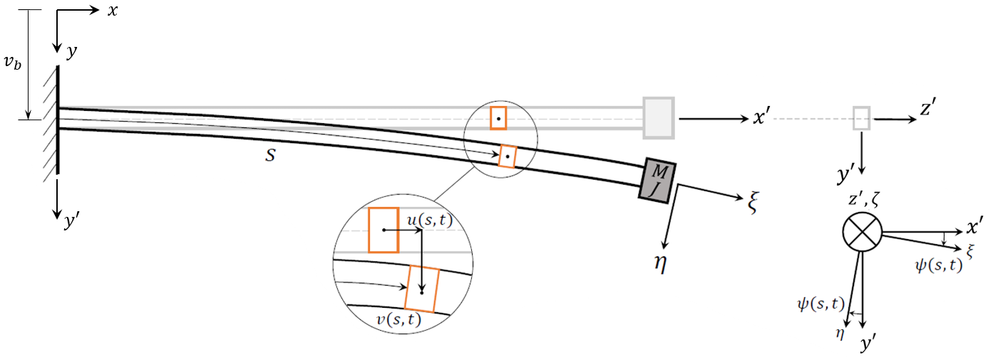
(a)

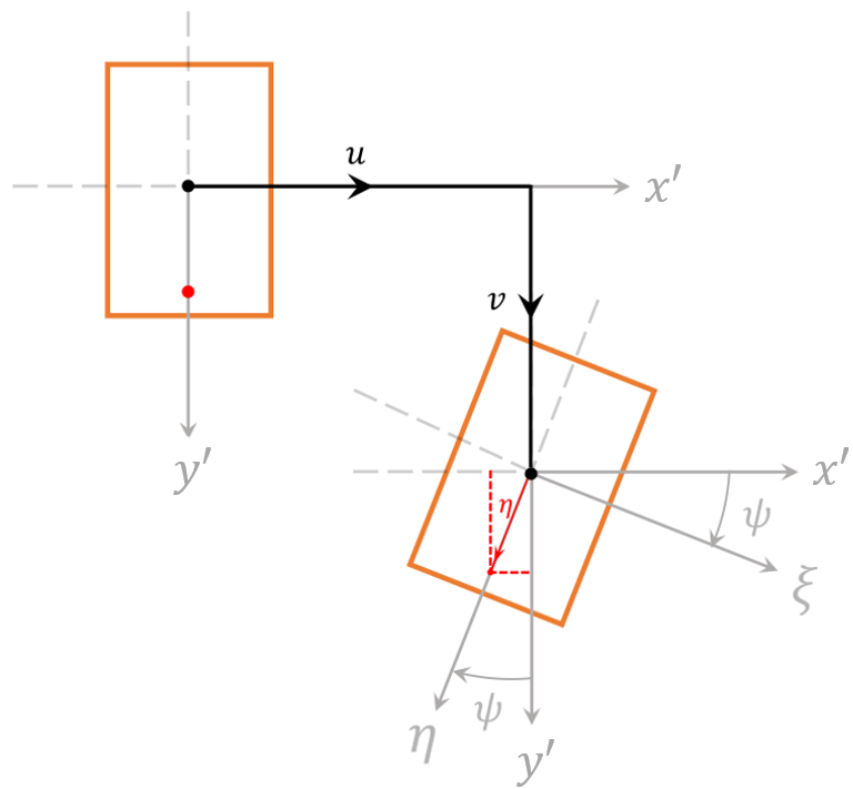
(b)

Figure 1: (a) In-plane kinematics of the cantilever beam subject to a base displacement $v_{b}(t)$ with respect to an inertial coordinate system $(x,y,z)$. The terms $u(s,t)$ and $v(s,t)$ denote, respectively, the axial and vertical displacements with respect to a $(x^{\prime},y^{\prime},z^{\prime})$ coordinate system attached to the base, and $\psi(s,t)$ is the rotation angle about the $z^{\prime}$-axis. (b) The total deformation of an arbitrary (red) point, composed of an axial displacement $u$ and vertical displacement $v$, as well as the displacement due to rotation $\psi$.

Therefore, the total displacement and velocity of an arbitrary point of the beam with respect to the inertial coordinate system takes the form:

r $$=\left(u-\eta\,\sin(\psi)\right)\,\textbf{e}_{x}+\left(v+{{v_{b}}}+\eta\,\cos(\psi)\right)\,\textbf{e}_{y},$$ (2)

$$\frac{\partial{\textbf{r}}}{\partial{t}} =\left(\frac{\partial{u}}{\partial{t}}-\eta\,\frac{\partial{\psi}}{\partial{t}}\,\cos(\psi)\right)\,\textbf{e}_{x}+\left(\frac{\partial{v}}{\partial{t}}+\frac{\partial{{{v_{b}}}}}{\partial{t}}-\eta\,\frac{\partial{\psi}}{\partial{t}}\,\sin(\psi)\right)\,\textbf{e}_{y}.$$ (3)

We also let an arbitrary element $CD$ with initial length $ds$ on the neutral axis, located at a distance $s$ from the origin $O$ of the moving system $(x^{\prime},y^{\prime},z^{\prime})$, to deformation to an updated configuration $C^{*}D^{*}$ (see Fig. 2). The displacement components of points $C$ and $D$ are denoted by the pairs $(u,v)$ and $(u+du,v+dv)$, respectively. The axial strain $e(s,t)$ at point $C$ is given by

$$e =\frac{ds^{*}-ds}{ds}=\frac{\sqrt{(ds+du)^{2}+dv^{2}}-ds}{ds}=\sqrt{(1+\frac{\partial{u}}{\partial{s}})^{2}+(\frac{\partial{v}}{\partial{s}})^{2}}-1.$$ (4)

Applying the inextensionality assumption, i.e. $e=0$, (4) becomes

$$1+\frac{\partial{u}}{\partial{s}}=\left(1-(\frac{\partial{v}}{\partial{s}})^{2}\right)^{1/2}.$$ (5)

Moreover, based on the assumption of negligible vertical shear strains, and using (5), we have the following expression for the rotation:

$$\psi=\text{tan}^{-1}\frac{\frac{\partial{v}}{\partial{s}}}{1+\frac{\partial{u}}{\partial{s}}}=\text{tan}^{-1}\frac{\frac{\partial{v}}{\partial{s}}}{\left(1-(\frac{\partial{v}}{\partial{s}})^{2}\right)^{1/2}}.$$ (6)

Using the expansion $\tan^{-1}(x)=x-\frac{1}{3}x^{3}+\cdots$, the curvature can be approximated up to third-order terms as

$$\psi =\frac{\partial{v}}{\partial{s}}(1-(\frac{\partial{v}}{\partial{s}})^{2})^{-1/2}-\frac{1}{3}(\frac{\partial{v}}{\partial{s}})^{3}(1-(\frac{\partial{v}}{\partial{s}})^{2})^{-3/2}+\cdots$$

$$\simeq\frac{\partial{v}}{\partial{s}}(1+\frac{1}{2}(\frac{\partial{v}}{\partial{s}})^{2})-\frac{1}{3}(\frac{\partial{v}}{\partial{s}})^{3}\simeq\frac{\partial{v}}{\partial{s}}+\frac{1}{6}(\frac{\partial{v}}{\partial{s}})^{3}\$$ (7)

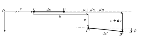
Figure 2: Deformation of an arbitrary element of the beam. The initial configuration $CD$ translates, rotates and elongates to an updated configuration $C^{*}D^{*}$.

Therefore, the angular velocity and curvature of the beam, i.e. $\frac{\partial{\psi}}{\partial{t}}$ and $\frac{\partial{\psi}}{\partial{s}}$, respectively, can be approximated as:

$$\frac{\partial{\psi}}{\partial{t}}\simeq\frac{\partial^{2}{v}}{\partial{t}\partial{s}}+\frac{1}{2}\,\frac{\partial^{2}{v}}{\partial{t}\partial{s}}\,(\frac{\partial{v}}{\partial{s}})^{2}\simeq\frac{\partial^{2}{v}}{\partial{t}\partial{s}}(1+\frac{1}{2}(\frac{\partial{v}}{\partial{s}})^{2}),$$ (8)

$$\frac{\partial{\psi}}{\partial{s}}\simeq\frac{\partial^{2}{v}}{\partial{s}^{2}}+\frac{1}{2}\frac{\partial^{2}{v}}{\partial{s}^{2}}(\frac{\partial{v}}{\partial{s}})^{2}\simeq\frac{\partial^{2}{v}}{\partial{s}^{2}}(1+\frac{1}{2}(\frac{\partial{v}}{\partial{s}})^{2}).$$ (9)

By the Euler-Bernoulli beam assumptions a slender beam without vertical shear strains, the strain-curvature relationship takes the form

$$\varepsilon(s,t)=-\eta\,\frac{\partial{\psi}(s,t)}{\partial{s}}$$ (10)

2.2 Linear Viscoelasticity: Boltzmann Superposition Principle

In this section, we start with a bottom-up derivation of our rheological building block, i.e., the Scott-Blair model through the Boltzmann superposition principle. Then, in a top-bottom fashion, we demonstrate how the fractional Kelvin-Voigt model is obtained from a general distributed-order form. Assuming linear viscoelasticity, and applying a small step strain increase, denoted by $\delta\varepsilon(t)$, at a given time $t=\tau_{1}$, the resulting stress in the material is given by:

$$\sigma(t)=G(t-\tau_{1})\delta\varepsilon(\tau_{1}),\quad t>\tau_{1},$$ (11)

where $G(t)$ denotes the relaxation function. The Boltzmann superposition principle states that resulting stresses from distinct applied small strains are additive. Therefore, the total tensile stress of the specimen at time $t$ is obtained from the superposition of infinitesimal changes in strain at some prior time $\tau_{j}$, given as $G(t-\tau_{j})\delta\varepsilon(\tau_{j})$. Therefore,

$$\sigma(t)=\sum_{\tau_{j}<t}G(t-\tau_{j})\frac{\delta\varepsilon(\tau_{j})}{\delta\tau_{j}}\delta\tau_{j},$$ (12)

where the limiting case $\delta\tau_{j}\rightarrow 0$ yields the following integral form:

$$\sigma(t)=\int_{-\infty}^{t}G(t-\tau)\,\dot{\varepsilon}(\tau)\,d\tau,$$ (13)

where $\dot{\varepsilon}$ denotes the strain rate.

2.2.1 Exponential Relaxation (Classical Models) vs. Power-Law Relaxation (Fractional Models)

The relaxation function $G(t)$ is traditionally expressed as the summation of exponential functions with different exponents and constants, which yields the so-called generalized Maxwell form as:

$$G(t)=\sum C_{i}e^{-t/\tau_{i}}.$$ (14)

For the simple case of a single exponential term (a single Maxwell branch), we have $G(t)=Ee^{-t/\tau}$. Therefore, in the case of zero initial strain $(\varepsilon(0)=0)$, we have:

$$\sigma(t)=E\int_{0}^{t}e^{-(t-\tilde{t})/\tau}\,\dot{\varepsilon}(\tilde{t})\,d\tilde{t},$$ (15)

which solves the integer-order differential equation $\frac{\partial{\varepsilon}}{\partial{t}}=\frac{1}{E}\frac{\partial{\sigma}}{\partial{t}}+\frac{1}{\eta}\sigma$, where the relaxation time constant $\tau=\eta/E$ is obtained from experimental observations. The Maxwell model is in fact a combination of purely elastic and purely viscous elements in series, as illustrated in Fig. 3.

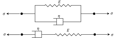
Figure 3: Classical viscoelastic models as a combination of spring (purely elastic) and dash-pot (purely viscous) elements. Kelvin-Voigt (top) and Maxwell (bottom) rheological models.

By letting the relaxation function (kernel) in (13) have a modulated power-law form $G(t)=E_{\alpha}\,g(\alpha)(\,t-\tau\,)^{-\alpha}$, equation (13) for the stress takes the following form,

$$\sigma(t) =E_{\alpha}\,g(\alpha)\,\int_{-\infty}^{t}\frac{\dot{\varepsilon}(\tau)}{(\,t-\tau\,)^{\alpha}}\,d\tau.$$ (16)

where $E_{\alpha}$ denotes a pseudo-constant with units $[Pa.s^{\alpha}]$. If we choose the modulation $g(\alpha)=\frac{1}{\Gamma(1-\alpha)}$, then the integro-differential operator (16) gives the Liouville-Weyl fractional derivative [52]. Although the lower integration limit of (16) is taken as $-\infty$, under hypothesis of causal histories, which states that the viscoelastic body is quiescent for all time prior to some starting point $t=0$, (16) can be re-written as

$$\sigma(t) =\varepsilon(0^{+})\,\frac{E_{\alpha}\,g(\alpha)}{t^{\alpha}}+E_{\alpha}\,g(\alpha)\,\int_{0}^{t}\frac{\dot{\varepsilon}}{(\,t-\tau\,)^{\alpha}}\,d\tau,$$

$$=\varepsilon(0^{+})\,\frac{E_{\alpha}\,g(\alpha)}{t^{\alpha}}+E_{\alpha}\,\prescript{C}{0}{\mathcal{D}}_{t}^{\alpha}\,\varepsilon,$$

$$=E_{\alpha}\,\prescript{RL}{0}{\mathcal{D}}_{t}^{\alpha}\,\varepsilon,$$ (17)

where $\prescript{C}{0}{\mathcal{D}}_{t}^{\alpha}$ and $\prescript{RL}{0}{\mathcal{D}}_{t}^{\alpha}$ denote, respectively, the Caputo and Riemann-Liouville fractional derivatives [52]. Both definitions are equivalent here due to homogeneous initial conditions for the strain.

Remark 1

The constitutive equation (2.2.1) can be thought of as an interpolation between a pure elastic (spring) and a pure viscous (dash-pot) elements, i.e., the Scott Blair element [53, 54, 55, 21]. It should be noted that in the limiting cases of $\alpha\rightarrow 0$ and $\alpha\rightarrow 1$, the relation (2.2.1) recovers the corresponding equations for spring and dash-pot, respectively.

2.2.2 Multi-Scale Power-Laws, Distributed-Order Models

In the most general sense, materials intrinsically possess a spectrum of power-law relaxations, and therefore we need a distributed-order representation for the stress-strain relationship. Consequently, the relaxation function $G(t)$ in (13) does not only contain a single power-law as in (16), but rather a distribution over a range of values. Considering nonlinear viscoelasticity with material heterogeneities, the distributed order constitutive equations over $t>0$ with orders $\alpha\in[\alpha_{min},\alpha_{max}]$ and $\beta\in[\beta_{min},\beta_{max}]$ can be expressed in the general form as

$$\int_{\beta_{min}}^{\beta_{max}}\Phi(\beta;x,t,\sigma)\prescript{*}{0}{\mathcal{D}}_{t}^{\beta}\sigma(t)\,d\beta=\int_{\alpha_{min}}^{\alpha_{max}}\Psi(\alpha;x,t,\varepsilon)\prescript{*}{0}{\mathcal{D}}_{t}^{\alpha}\varepsilon(t)d\alpha,$$ (18)

in which the prescript $*$ stands for any type of fractional derivative, and initial conditions also depending on such definitions. The functions $\Phi(\beta;x,t,\sigma)$ and $\Psi(\alpha;x,t,\varepsilon)$ can be thought of as distribution functions, where $\alpha\mapsto\Psi(\alpha;x,t,\varepsilon)$ and $\beta\mapsto\Phi(\beta;x,t,\sigma)$ are continuous mappings in $[\alpha_{min},\alpha_{max}]$ and $[\beta_{min},\beta_{max}]$. Furthermore, the dependence of the distributions on the (thermodynamically) conjugate pair $(\sigma,\varepsilon)$ introduces the notion of nonlinear viscoelasticity, and the dependence on a material coordinate $x$ induces material heterogeneties in space.

Remark 2

The pairs ($\alpha_{min}$, $\alpha_{max}$) and ($\beta_{min}$, $\beta_{max}$) are only the theoretical lower and upper terminals in the definition of distributed order models. In general, the distribution function $\Phi(\beta;x,t,\sigma)$ and $\Psi(\alpha;x,t,\varepsilon)$ can arbitrarily confine the domain of integration in each realization of practical rheological problems and material design. If we let the distribution be summation of some delta functions, then, the distributed order model becomes the following multi-term model:

$$\left(1+\sum_{k=1}^{p_{\sigma}}\,a_{k}\,\prescript{}{0}{\mathcal{D}}_{t}^{\beta_{k}}\right)\,\sigma(t)=\left(c+\sum_{k=1}^{p_{\varepsilon}}\,b_{k}\,\prescript{}{0}{\mathcal{D}}_{t}^{\alpha_{k}}\right)\,\varepsilon(t).$$

In order to obtain the fractional Kelvin-Voigt model, we let $\Phi(\beta)=\delta(\beta)$ and $\Psi(\alpha)=E_{\infty}\delta(\alpha)+E_{\alpha}\delta(\alpha-\alpha_{0})$ in (18), and therefore,

$$\sigma(t)=E_{\infty}\,\varepsilon(t)+E_{\alpha}\,\prescript{RL}{0}{\mathcal{D}}_{t}^{\alpha}\,\varepsilon(t),\quad{\alpha\in(0,1).}$$ (19)

2.3 Extended Hamilton’s Principle

We derive the equations of motion by employing the extended Hamilton’s principle

$$\int_{t_{1}}^{t_{2}}\left(\delta T-\delta W\right)\,dt=0,$$

where $\delta T$ and $\delta W$ denote the variations of kinetic energy and total work [56]. The only source of external input to our system of interest is the base excitation, which is linearly superposed to the beam’s vertical displacement $v(t)$, and therefore contributes to the kinetic energy taken in the inertial (Lagrangian) coordinate system. Hence, the total work only contains the internal work done by the stress state, with the variation expressed as [57]

$$\delta W=\int_{\mathbb{V}}\sigma\,\delta\varepsilon\,dv,$$ (20)

where the integral is taken over the whole system volume $\mathbb{V}$.

Remark 3

It is remarked in (1) that the fractional Scott-Blair elements exhibit both elasticity and viscosity behaviors. There have been attempts in the literature to separate the conservative (elastic) and non-conservative (viscous) parts of fractional constitutive equations at the free-energy level [58]. However, we note this separation in the time domain is not trivial for sophisticated fractional constitutive equations, and therefore we choose to formulate our problem in terms of the total work in order to avoid such additional complexities.

The full derivation of the governing equation using the extended Hamilton’s principle is given in A. We recall that $M$ and $J$ are the mass and rotatory inertia of the lumped mass at the tip of beam, $\rho$ is the mass per unit length of the beam, $I=\int_{A}\eta^{2}\,dA$, and let $m=\frac{\rho}{E_{\infty}\,I}$ and $E_{r}=\frac{E_{\alpha}}{E_{\infty}}$. We approximate the nonlinear terms up to third order and use the following dimensionless variables

$$s^{*}=\frac{s}{L},\,\,v^{*} =\frac{v}{L},\,\,t^{*}=t\left(\frac{1}{mL^{4}}\right)^{1/2},\,\,E_{r}^{*}=E_{r}\left(\frac{1}{mL^{4}}\right)^{\alpha/2},\,\,J^{*}=\frac{J}{\rho L^{3}},\,\,M^{*}=\frac{M}{\rho L},\,\,{{v_{b}}}^{*}=\frac{{{v_{b}}}}{L},$$

and derive the strong form of the equation of motion. Therefore, by choosing a proper function space $V$, the problem reads as: find $v\in V$ such that

$$\frac{\partial^{2}{v}}{\partial{t}^{2}}+\frac{\partial^{2}}{\partial{s}^{2}}\left(\frac{\partial^{2}{v}}{\partial{s}^{2}}+\frac{\partial^{2}{v}}{\partial{s}^{2}}(\frac{\partial{v}}{\partial{s}})^{2}\right.\left.+E_{r}\prescript{RL}{0}{\mathcal{D}}_{t}^{\alpha}\,\Big{[}\frac{\partial^{2}{v}}{\partial{s}^{2}}(1+\frac{1}{2}(\frac{\partial{v}}{\partial{s}})^{2})\Big{]}+\frac{1}{2}E_{r}(\frac{\partial{v}}{\partial{s}})^{2}\,\prescript{RL}{0}{\mathcal{D}}_{t}^{\alpha}\,\frac{\partial^{2}{v}}{\partial{s}^{2}}\right)$$

$$-\frac{\partial}{\partial{s}}\left(\frac{\partial{v}}{\partial{s}}\,(\frac{\partial^{2}{v}}{\partial{s}^{2}})^{2}+E_{r}\frac{\partial{v}}{\partial{s}}\,\frac{\partial^{2}{v}}{\partial{s}^{2}}\,\prescript{RL}{0}{\mathcal{D}}_{t}^{\alpha}\,\frac{\partial^{2}{v}}{\partial{s}^{2}}\right)=-\ddot{{{v_{b}}}},$$ (21)

which is subject to the following boundary conditions:

$$v\,\Big{|}_{s=0}=\frac{\partial{v}}{\partial{s}}\,\Big{|}_{s=0}=0,$$

$$J\left(\frac{\partial^{3}{v}}{\partial{t}^{2}\partial{s}}(1+(\frac{\partial{v}}{\partial{s}})^{2})+\frac{\partial{v}}{\partial{s}}(\frac{\partial^{2}{v}}{\partial{s}\partial{t}})^{2}\right)$$

$$+\left(\frac{\partial^{2}{v}}{\partial{s}^{2}}+\frac{\partial^{2}{v}}{\partial{s}^{2}}(\frac{\partial{v}}{\partial{s}})^{2}+E_{r}\,\prescript{RL}{0}{\mathcal{D}}_{t}^{\alpha}\,\Big{[}\frac{\partial^{2}{v}}{\partial{s}^{2}}(1+\frac{1}{2}(\frac{\partial{v}}{\partial{s}})^{2})\Big{]}\right.\left.+\frac{1}{2}E_{r}\,(\frac{\partial{v}}{\partial{s}})^{2}\,\prescript{RL}{0}{\mathcal{D}}_{t}^{\alpha}\,\frac{\partial^{2}{v}}{\partial{s}^{2}}\right)\,\,\Bigg{|}_{s=1}=0,$$

$$M(\frac{\partial^{2}{v}}{\partial{t}^{2}}\!+\!\ddot{{{v_{b}}}})\!-\!\frac{\partial{v}}{\partial{s}}\left(\frac{\partial^{2}{v}}{\partial{s}^{2}}\!+\!\frac{\partial^{2}{v}}{\partial{s}^{2}}(\frac{\partial{v}}{\partial{s}})^{2}+E_{r}\,\prescript{RL}{0}{\mathcal{D}}_{t}^{\alpha}\,\Big{[}\frac{\partial^{2}{v}}{\partial{s}^{2}}(1\!+\!\frac{1}{2}(\frac{\partial{v}}{\partial{s}})^{2})\Big{]}\!+\!\frac{1}{2}E_{r}\,(\frac{\partial{v}}{\partial{s}})^{2}\,\prescript{RL}{0}{\mathcal{D}}_{t}^{\alpha}\,\frac{\partial^{2}{v}}{\partial{s}^{2}}\right)$$

$$+\left(\frac{\partial{v}}{\partial{s}}\,(\frac{\partial^{2}{v}}{\partial{s}^{2}})^{2}+E_{r}\,\frac{\partial{v}}{\partial{s}}\,\frac{\partial^{2}{v}}{\partial{s}^{2}}\,\prescript{RL}{0}{\mathcal{D}}_{t}^{\alpha}\,\frac{\partial^{2}{v}}{\partial{s}^{2}}\right)\,\,\Bigg{|}_{s=1}=0.$$ (22)

2.4 Weak Formulation

The common practice in analysis of numerical methods for PDEs are mostly concerned with linear equations. Analyses for linear PDEs are well-developed and well-defined, however they are still scarce for nonlinear PDEs. The linear theories are usually applicable to nonlinear problems if the solution is sufficiently smooth [59]. We do not intend to investigate/develop analysis for our proposed nonlinear model. Instead, by assuming smooth solution, we employ linear theories in our analysis. Let $v:\mathbb{R}^{1+1}\rightarrow\mathbb{R}$ for $\alpha\in(0,1)$ and $\Omega=[0,T]\times[0,L]$. Here, we construct the solution space, $\mathcal{B}^{\alpha}\,(\Omega)$, endowed with proper norms [43], in which the corresponding weak form of (2.3) can be formulated. If we recall the equation (2.3) as E, then:

$$\mathcal{B}^{\alpha}\,(\Omega):=\Big{\{}v\in\prescript{l}{0}{H}^{\alpha}(\Omega)\,\Big{|}\int_{\Omega}E\,d\Omega<\infty\Big{\}}$$ (23)

where

$$\prescript{l}{0}{H}^{\alpha}(\Omega)=\prescript{l}{0}{H}^{\alpha}\,\Big{(}I;L^{2}\,(\Omega)\Big{)}\cap L^{2}(I;\prescript{}{0}{H}^{2}(\Omega)),\qquad\prescript{}{0}{H}^{2}(\Omega)=\Big{\{}v\in{H}^{2}(\Omega)\,\Big{|}\,\,v\,\Big{|}_{s=0}=\frac{\partial{v}}{\partial{s}}\,\Big{|}_{s=0}=0\Big{\}}$$

We obtain the weak form of the problem by multiplying the strong form (2.3) with proper test functions $\tilde{v}(s)\in\mathcal{B}^{\alpha}(\Omega)$ and integrating over the dimensionless spatial computational domain $\Omega_{s}=[0,1]$. The test functions satisfy the boundary conditions, i.e. $\tilde{v}(0)=\frac{\partial{\tilde{v}}}{\partial{s}}(0)=0$. Therefore, we obtain:

$$\!\int_{0}^{1}\!\frac{\partial^{2}{v}}{\partial{t}^{2}}\tilde{v}ds\!+\!\!\int_{0}^{1}\!\frac{\partial^{2}}{\partial{s}^{2}}\left(\frac{\partial^{2}{v}}{\partial{s}^{2}}\!+\!\frac{\partial^{2}{v}}{\partial{s}^{2}}(\frac{\partial{v}}{\partial{s}})^{2}\!+\!E_{r}\prescript{RL}{0}{\mathcal{D}}_{t}^{\alpha}\Big{[}\frac{\partial^{2}{v}}{\partial{s}^{2}}(1\!+\!\frac{1}{2}(\frac{\partial{v}}{\partial{s}})^{2})\Big{]}\!+\!\frac{1}{2}E_{r}(\frac{\partial{v}}{\partial{s}})^{2}\prescript{RL}{0}{\mathcal{D}}_{t}^{\alpha}\frac{\partial^{2}{v}}{\partial{s}^{2}}\right)\tilde{v}ds$$

$$-\int_{0}^{1}\frac{\partial}{\partial{s}}\left(\frac{\partial{v}}{\partial{s}}\,(\frac{\partial^{2}{v}}{\partial{s}^{2}})^{2}+E_{r}\frac{\partial{v}}{\partial{s}}\,\frac{\partial^{2}{v}}{\partial{s}^{2}}\,\prescript{RL}{0}{\mathcal{D}}_{t}^{\alpha}\,\frac{\partial^{2}{v}}{\partial{s}^{2}}\right)\,\tilde{v}\,ds=-\int_{0}^{1}\ddot{{{v_{b}}}}\,\tilde{v}\,ds.$$ (24)

Integrating the above equation by parts, we obtain:

$$\frac{\partial^{2}}{\partial{t}^{2}}\int_{0}^{1}v\tilde{v}ds\!+\!\int_{0}^{1}\left(\frac{\partial^{2}{v}}{\partial{s}^{2}}+\frac{\partial^{2}{v}}{\partial{s}^{2}}(\frac{\partial{v}}{\partial{s}})^{2}\!+\!E_{r}\prescript{RL}{0}{\mathcal{D}}_{t}^{\alpha}\Big{[}\frac{\partial^{2}{v}}{\partial{s}^{2}}(1\!+\!\frac{1}{2}(\frac{\partial{v}}{\partial{s}})^{2})\Big{]}\!+\!\frac{1}{2}E_{r}(\frac{\partial{v}}{\partial{s}})^{2}\prescript{RL}{0}{\mathcal{D}}_{t}^{\alpha}\frac{\partial^{2}{v}}{\partial{s}^{2}}\right)\frac{\partial^{2}{\tilde{v}}}{\partial{s}^{2}}ds$$

$$+\int_{0}^{1}\left(\frac{\partial{v}}{\partial{s}}\,(\frac{\partial^{2}{v}}{\partial{s}^{2}})^{2}+E_{r}\frac{\partial{v}}{\partial{s}}\,\frac{\partial^{2}{v}}{\partial{s}^{2}}\,\prescript{RL}{0}{\mathcal{D}}_{t}^{\alpha}\,\frac{\partial^{2}{v}}{\partial{s}^{2}}\right)\,\frac{\partial{\tilde{v}}}{\partial{s}}\,ds+M(\frac{\partial^{2}{v}}{\partial{t}^{2}}+\ddot{{{v_{b}}}})\,\tilde{v}\,\Big{|}_{s=1}+J\left(\frac{\partial^{3}{v}}{\partial{t}^{2}\partial{s}}(1+(\frac{\partial{v}}{\partial{s}})^{2})+\frac{\partial{v}}{\partial{s}}(\frac{\partial^{2}{v}}{\partial{t}\partial{s}})^{2}\right)\frac{\partial{\tilde{v}}}{\partial{s}}\,\Big{|}_{s=1}$$

$$=-\ddot{{{v_{b}}}}\,\int_{0}^{1}\tilde{v}\,ds.$$ (25)

By rearranging the terms, we get

$$\frac{\partial^{2}}{\partial{t}^{2}}\,\left(\int_{0}^{1}v\,\tilde{v}\,ds+M\,v\,\tilde{v}\,\Big{|}_{s=1}+J\,\frac{\partial{v}}{\partial{s}}\,\frac{\partial{\tilde{v}}}{\partial{s}}\,\Big{|}_{s=1}\right)+J\left(\frac{\partial^{3}{v}}{\partial{t}^{2}\partial{s}}(\frac{\partial{v}}{\partial{s}})^{2}+\frac{\partial{v}}{\partial{s}}\ (\frac{\partial^{2}{v}}{\partial{t}\partial{s}})^{2}\right)\frac{\partial{\tilde{v}}}{\partial{s}}\,\Big{|}_{s=1}+\int_{0}^{1}\frac{\partial^{2}{v}}{\partial{s}^{2}}\,\frac{\partial^{2}{\tilde{v}}}{\partial{s}^{2}}\,ds$$

$$+E_{r}\int_{0}^{1}\prescript{RL}{0}{\mathcal{D}}_{t}^{\alpha}\,\Big{[}\frac{\partial^{2}{v}}{\partial{s}^{2}}\Big{]}\,\,\frac{\partial^{2}{\tilde{v}}}{\partial{s}^{2}}\,ds+\int_{0}^{1}\frac{\partial^{2}{v}}{\partial{s}^{2}}(\frac{\partial{v}}{\partial{s}})^{2}\,\,\frac{\partial^{2}{\tilde{v}}}{\partial{s}^{2}}\,ds+\int_{0}^{1}\frac{\partial{v}}{\partial{s}}\,(\frac{\partial^{2}{v}}{\partial{s}^{2}})^{2}\,\,\frac{\partial{\tilde{v}}}{\partial{s}}\,ds+\frac{E_{r}}{2}\int_{0}^{1}\prescript{RL}{0}{\mathcal{D}}_{t}^{\alpha}\,\Big{[}\frac{\partial^{2}{v}}{\partial{s}^{2}}(\frac{\partial{v}}{\partial{s}})^{2}\Big{]}\,\,\frac{\partial^{2}{\tilde{v}}}{\partial{s}^{2}}\,ds$$

$$\!+\!\frac{E_{r}}{2}\int_{0}^{1}(\frac{\partial{v}}{\partial{s}})^{2}\prescript{RL}{0}{\mathcal{D}}_{t}^{\alpha}\Big{[}\frac{\partial^{2}{v}}{\partial{s}^{2}}\Big{]}\frac{\partial^{2}{\tilde{v}}}{\partial{s}^{2}}ds\!+\!E_{r}\int_{0}^{1}\frac{\partial{v}}{\partial{s}}\frac{\partial^{2}{v}}{\partial{s}^{2}}\prescript{RL}{0}{\mathcal{D}}_{t}^{\alpha}\Big{[}\frac{\partial^{2}{v}}{\partial{s}^{2}}\Big{]}\frac{\partial{\tilde{v}}}{\partial{s}}ds=-\ddot{{{v_{b}}}}\left(\int_{0}^{1}\tilde{v}ds\!+\!M\tilde{v}\Big{|}_{s=1}\right).$$ (26)

2.5 Assumed Mode: A Spectral Approximation in Space

We employ the following modal discretization to obtain a reduced-order model of the beam. Therefore,

$$v(s,t)\simeq v_{N}(s,t)=\sum_{n=1}^{N}q_{n}(t)\,\phi_{n}(s),$$ (27)

where the spatial functions $\phi_{n}(s),\,\,n=1,2,\cdots,N$ are assumed a priori and the temporal functions $q_{n}(t),\,\,n=1,2,\cdots,N$ are the unknown modal coordinates. The assumed modes $\phi_{n}(s)$ in (27) are obtained in D, by solving the corresponding linear eigenvalue problem of our nonlinear model. Subsequently, we construct the proper finite dimensional spaces of basis/test functions as:

$$V_{N}=\tilde{V}_{N}=span\,\Big{\{}\,\,\phi_{n}(x):n=1,2,\cdots,N\,\,\Big{\}}.$$ (28)

Since $V_{N}=\tilde{V}_{N}\subset V=\tilde{V}$, problem (2.4) read as: find $v_{N}\in V_{N}$ such that

$$\frac{\partial^{2}}{\partial{t}^{2}}\left(\int_{0}^{1}v_{N}\tilde{v}_{N}ds\!+\!Mv_{N}\tilde{v}_{N}\Big{|}_{s=1}\!+\!J\frac{\partial{{v}_{N}}}{\partial{s}}\frac{\partial{\tilde{v}_{N}}}{\partial{s}}\,\Big{|}_{s=1}\right)\!+\!J\left(\frac{\partial^{3}{{v}_{N}}}{\partial{t}^{2}\partial{s}}(\frac{\partial{{v}_{N}}}{\partial{s}})^{2}\!+\!\frac{\partial{{v}_{N}}}{\partial{s}}(\frac{\partial^{2}{{v}_{N}}}{\partial{t}\partial{s}})^{2}\right)\frac{\partial{\tilde{v}_{N}}}{\partial{s}}\Big{|}_{s=1}+\int_{0}^{1}\frac{\partial^{2}{{v}_{N}}}{\partial{s}^{2}}\,\frac{\partial^{2}{\tilde{v}_{N}}}{\partial{s}^{2}}\,ds$$

$$+E_{r}\int_{0}^{1}\prescript{RL}{0}{\mathcal{D}}_{t}^{\alpha}\,\Big{[}\frac{\partial^{2}{{v}_{N}}}{\partial{s}^{2}}\Big{]}\,\,\frac{\partial^{2}{\tilde{v}_{N}}}{\partial{s}^{2}}\,ds+\int_{0}^{1}\frac{\partial^{2}{{v}_{N}}}{\partial{s}^{2}}(\frac{\partial{{v}_{N}}}{\partial{s}})^{2}\,\,\frac{\partial^{2}{\tilde{v}_{N}}}{\partial{s}^{2}}\,ds+\int_{0}^{1}\frac{\partial{{v}_{N}}}{\partial{s}}\,(\frac{\partial^{2}{{v}_{N}}}{\partial{s}})^{2}\,\,\frac{\partial{\tilde{v}_{N}}}{\partial{s}}\,ds$$

$$+\frac{E_{r}}{2}\int_{0}^{1}\prescript{RL}{0}{\mathcal{D}}_{t}^{\alpha}\,\Big{[}\frac{\partial^{2}{{v}_{N}}}{\partial{s}^{2}}(\frac{\partial{v_{N}}}{\partial{s}})^{2}\Big{]}\,\,\frac{\partial^{2}{\tilde{v}_{N}}}{\partial{s}^{2}}\,ds+\frac{E_{r}}{2}\int_{0}^{1}(\frac{\partial{{v}_{N}}}{\partial{s}})^{2}\,\prescript{RL}{0}{\mathcal{D}}_{t}^{\alpha}\,\Big{[}\frac{\partial^{2}{{v}_{N}}}{\partial{s}^{2}}\Big{]}\,\,\frac{\partial^{2}{\tilde{v}_{N}}}{\partial{s}^{2}}\,ds$$

$$+E_{r}\int_{0}^{1}\frac{\partial{{v}_{N}}}{\partial{s}}\,\frac{\partial^{2}{v_{N}}}{\partial{s}^{2}}\,\prescript{RL}{0}{\mathcal{D}}_{t}^{\alpha}\,\Big{[}\frac{\partial^{2}{{v}_{N}}}{\partial{s}^{2}}\Big{]}\,\,\frac{\partial{\tilde{v}_{N}}}{\partial{s}}\,ds=-\ddot{{{v_{b}}}}\left(\int_{0}^{1}\tilde{v}_{N}\,ds+M\,\tilde{v}_{N}\,\Big{|}_{s=1}\right),$$ (29)

for all $\tilde{v}_{N}\in\tilde{V}_{N}$.

2.6 Single Mode Approximation

In general, the modal discretization (27) in (2.5) leads to a coupled nonlinear system of fractional ordinary differential equations. We note that while the fractional operators already impose numerical challenges, these are increased by the presence of nonlinearities, leading to failure of existing numerical schemes. However, without loss of generality, we can assume that only one mode (primary mode) of motion is involved in the dynamics of system of interest.

2.6.1 Why is single-mode approximation useful?

Although single-mode approximations are simplistic in nature, they encapsulate the most fundamental dynamics and the highest energy mode in the motion of nonlinear systems. Furthermore, as shown by numerous studies below, such approximation also proved capable of capturing the complex behavior of structures.

Azrar et al. [60] demonstrated sufficient approximations of single- and multi-modal representation for the nonlinear forced vibration of a simply supported beam under a uniform harmonic distributed force. Tseng and Dugundji [61] showed similar results between single and two mode approximations for nonlinear vibrations of clamped-clamped beams far from the crossover region. Loutridis et al. [62] implemented a crack detection method for beams using a single-degree-of-freedom system with time varying stiffness. In [63], the effects of base stiffness and attached mass on the nonlinear, planar flexural free vibrations of beams were studied. Lestari and Hanagud [64] studied the nonlinear free vibrations of buckled beams with elastic end constraints, where the single-mode assumption led to a closed-form solution in terms of elliptic functions.

Of particular interest, Habtour et al. [3] detected and validated the response of a nonlinear cantilever beam subject to softening due to local stress-induced, early fatigue damage precursors prior to crack formation. Their findings demonstrate that the pragmatism of a single-mode approximation provides sufficient sensitivity of the amplitude response with respect to the nonlinear stiffness, making their framework an effective practical tool for early fatigue detection. We also refer the reader to [65, 66, 67, 68] for additional applications.

Therefore, we let the anomalous dynamics of our system be driven by the fractional-order $\alpha$, and following the aforementioned studies, we replace (27) with the one-mode discretization $v_{N}=q(t)\,\phi(s)$ (where we let $N=1$ and drop the subscript $1$ for simplicity). Upon substituting in (2.5), we obtain the unimodal governing equation of motion as (see B),

$$\mathcal{M}\ddot{q}+\mathcal{J}(\ddot{q}q^{2}\!+\!q{\dot{q}}^{2})+\mathcal{K}_{l}q+E_{r}\mathcal{C}_{l}\prescript{RL}{0}{\mathcal{D}}_{t}^{\alpha}q+2\mathcal{K}_{nl}\,q^{3}\!+\!\frac{E_{r}\mathcal{C}_{nl}}{2}\left(\prescript{RL}{0}{\mathcal{D}}_{t}^{\alpha}q^{3}\!+\!3q^{2}\prescript{RL}{0}{\mathcal{D}}_{t}^{\alpha}q\right)=-\mathcal{M}_{b}\ddot{{{v_{b}}}},$$ (30)

in which

$$\mathcal{M}=\int_{0}^{1}\phi^{2}\,ds+M\,\phi^{2}(1)+J\,{\phi^{\prime}}^{2}(1),\quad\mathcal{J}=J\,{\phi^{\prime}}^{4}(1),$$

$$\mathcal{K}_{l}=\mathcal{C}_{l}=\int_{0}^{1}{\phi^{\prime\prime}}^{2}\,\,ds,\quad\mathcal{K}_{nl}=\mathcal{C}_{nl}=\int_{0}^{1}{\phi^{\prime}}^{2}\,{\phi^{\prime\prime}}^{2}\,\,ds,\,\,\mathcal{M}_{b}=\int_{0}^{1}\phi\,ds+M\,\phi(1).$$ (31)

Remark 4

We note that one can isolate any mode of vibration $\phi_{n}(s),\,\,n=1,2,\cdots,N$ (and not necessarily the primary mode) by assuming that $\phi_{n}(s)$ is the only active one, and thus, end up with similar equation of motion as (30), where the coefficients in (2.6.1) are obtained based on the active mode $\phi_{n}(s)$. Therefore, we can also make sense of (30) as a decoupled equation of motion associated with mode $\phi_{n}(s)$, in which the interaction with other inactive modes is absent.

3 Linearized Equation: Direct Numerical Time Integration

We linearize our equation of motion for the cantilever beam by assuming small motions (see C), and obtain the following form:

$$\ddot{q}+E_{r}\,c_{l}\,\prescript{RL}{0}{\mathcal{D}}_{t}^{\alpha}q+k_{l}\,q={-m_{b}\ddot{v}_{b}},\quad q(0)=\frac{v(L,0)}{\phi(L)},\quad\dot{q}(0)=\frac{\dot{v}(L,0)}{\phi(L)}$$ (32)

with the coefficients

$$c_{l}=\frac{\mathcal{C}_{l}}{\mathcal{M}},\qquad k_{l}=\frac{\mathcal{K}_{l}}{\mathcal{M}},\qquad m_{b}=\frac{\mathcal{M}_{b}}{\mathcal{M}}.$$ (33)

The linearized, unimodal form (32) is equivalent to the vibration of a lumped fractional Kelvin-Voigt rheological element, and can be thought of as a fractional oscillator, shown schematically in Fig.4.

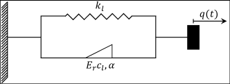
Figure 4: Lumped representation of the system as a fractional damper, with constants $E_{r}\,c_{l}$ and fractional order $\alpha$.

Let a uniform time-grid with $N$ time-steps of size $\Delta t$, such that $t_{n}=n\Delta t$, $n=0,\,1,\,\dots,\,N$. We employ the following equivalence relationship between the Riemann-Liouville and Caputo definitions:

$$\prescript{RL}{0}{\mathcal{D}}_{t}^{\alpha}q(t)=\prescript{C}{0}{\mathcal{D}}_{t}^{\alpha}q(t)+\frac{q(0)}{\Gamma(1-\alpha)t^{\alpha}}.$$ (34)

Substituting (34) into (32), evaluating both sides implicitly at $t=t_{n+1}$, and approximating the time-fractional Caputo derivative through an L1-difference scheme [49], we obtain:

$$\ddot{q}_{n+1}+E_{r}c_{l}\left[\frac{1}{\Delta t^{\alpha}\Gamma(2-\alpha)}\left(q_{n+1}-q_{n}+\mathcal{H}^{\alpha}q_{n+1}\right)+\frac{q_{0}}{\Gamma(1-\alpha)t^{\alpha}_{n+1}}\right]+k_{l}q_{n+1}=-m_{b}\ddot{v}_{b,n+1},$$ (35)

where $\mathcal{H}^{\alpha}_{k+1}=\sum^{n-1}_{j=0}=b_{j}(q_{n-j+1}-q_{n-j})$ represents the discretized history term, with $\alpha$-dependent convolution coefficients $b_{j}=(j+1)^{\alpha}-j^{\alpha}$. We approximate the acceleration $\ddot{q}_{n+1}$ and velocity $\dot{q}_{n+1}$ through a Newmark-$\beta$ method as follows:

$$\ddot{q}_{n+1}=a_{1}\left(q_{n+1}-q_{n}\right)-a_{2}\dot{q}_{n}-a_{3}\ddot{q}_{n},$$ (36)

$$\dot{q}_{n+1}=a_{4}\left(q_{n+1}-q_{n}\right)+a_{5}\dot{q}_{n}+a_{6}\ddot{q}_{n},$$ (37)

with approximation coefficients given by

$$a_{1}=\frac{1}{\beta\Delta t^{2}},\quad a_{2}=\frac{1}{\beta\Delta t},\quad a_{3}=\frac{1-2\beta}{2\beta},\quad a_{4}=\frac{\gamma}{\beta\Delta t^{2}},\quad a_{5}=\left(1-\frac{\gamma}{\beta}\right),\quad a_{6}=\left(1-\frac{\gamma}{2\beta}\right)\Delta t,$$

where we choose $\beta=0.5$, $\gamma=0.25$ for unconditional stability. Inserting (36) into (35), we obtain the following closed form for $q_{n+1}$:

$$q_{n+1}=\frac{\left(a_{1}+E^{*}\right)q_{n}+a_{2}\dot{q}_{n}+a_{3}\ddot{q}_{n}-m_{b}\ddot{v}_{b,n+1}-E^{*}\left[\mathcal{H}^{\alpha}_{n+1}+q_{0}\frac{(1-\alpha)}{(n+1)^{\alpha}}\right]}{a_{1}+E^{*}+k_{l}}$$ (38)

with $E^{*}=(E_{r}\,c_{l})/(\Delta t^{\alpha}\Gamma(2-\alpha))$. We observe that since the Newmark method is second-order accurate with respect to $\Delta t$, the overall accuracy is dominated by the accuracy of the $L1$ scheme, which is of $\mathcal{O}(\Delta t^{2-\alpha})$. We also observe that a discretization of a Caputo-variant of the FDE (32) is recovered if we remove the term $q_{0}(1-\alpha)/(n+1)^{\alpha}$ from (38).

We consider two numerical tests. In the first one, we solve the above system under harmonic base excitation, and in the second one, we consider a free-vibration response. For both tests, we set $E_{r}=1$ and consider the lumped mass at the tip, with $M=J=1$, that is, we utilize (121) for $\phi(s)$, which yields the coefficients $c_{l}=k_{l}=1.24$.

3.1 Harmonic Base Excitation

We solve (32) in the presence of base excitation in the harmonic form $v_{b}=a_{b}sin(\omega_{b}t)$, where $\omega_{b}\in[0.5,3.5]$ and $a_{b}=0.01$ denote, respectively, the base frequency and displacement amplitude. The coefficient $m_{b}=-0.042$ is calculated through (33) and (2.6.1). We employ homogeneous initial conditions, i.e., $q(0)=0$, $\dot{q}(0)=0$, and set the time $t\in(0,100]$, with step size $\Delta t=10^{-3}$. The maximum displacement amplitude after reaching the steady state response of the system is evaluated. Figure 5 illustrates the amplitude vs base frequency response with respect to varying fractional orders $\alpha$. We observe the existence of a critical point at $\omega_{b}=1$ that changes the dissipation nature of the fractional order parameter. Regarding the maximum observed amplitudes, increasing the fractional order in the range $\alpha\in[0.1,0.4]$, decreases and slightly shifts the amplitude peaks to higher (right) frequencies (an anomalous quality). On the other hand, as the fractional order is increased in the range $\alpha\in[0.5,0.6]$, the peak amplitudes slightly shift towards the lower (left) frequencies, which is also observed in standard systems with the increase of modal damping values.

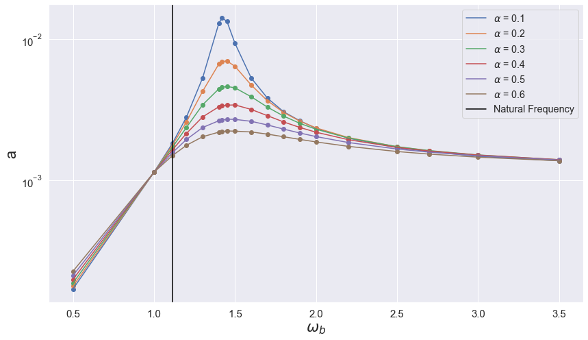
Figure 5: Anomalous change of the maximum amplitude vs frequency at the tip of the beam in presence of harmonic base excitation for different fractional order $\alpha$. The solid black line represents the standard, undamped natural frequency of the system.

3.2 Free Vibration

Following the observed anomalous amplitude vs. base frequency behaviors and presence of a critical point nearby the standard natural frequency of the system illustrated in Figure 5, we solve (32) in a free-vibration setting employing Riemann-Liouville and Caputo definitions, where we set $\ddot{v}_{b}=0$, and $q(0)=0.01$, $\dot{q}(0)=0$. Figure 6 (left) illustrates the obtained results for $q(t)$ for varying fractional orders using a Riemann-Liouville definition. We observe an $\alpha$-dependent amplitude decay, which converges to a classical integer-oder oscillator as $\alpha\to 1$. Furthermore, an anomalous transient region is observed at the short time-scale $t\in[0.1,\,1]$. On the other hand, in Figure 6 (right), anomalies are present at large time-scales through a (far-from-equilibrium) power-law relaxation, while the short-time behavior is “standard-like". Such contrast between the obtained results provides interesting insights towards modeling desired anomalous ranges in such power-law materials. By replacing the fractional damper with a classical integer-order one (see Fig.7), we notice that neither anomalous dynamics are present. The obtained results are in agreement with the power-law and exponential relaxation kernels described in Sec.2.2. We note that since the fractional element provides a constitutive interpolation between spring and dash-pot elements (see Sec.2.2 for more discussion and references), it contributes to both effective stiffness and damping ratio of the system, and therefore increasing values of $\alpha$ (decreasing stiffness), yield a reduction in the frequency response.

Fractional linear oscillators are also considered in [69] for systems with memory, where their interaction with a fluctuating environment causes the time evolution of the system to be intermittent. The authors in [69] apply the Koopman operator theory to the corresponding integer order system and then make a L$\grave{\text{e}}$vy transformation in time to recover long-term memory effects; they observe a power-law behavior in the amplitude decay of the system’s response. Such an anomalous decay rate has also been investigated in [70] for an extended theory of decay of classical vibrational models brought into nonlinear resonances. The authors report a “non-exponential" decay in variables describing the dynamics of the system in the presence of dissipation and also a sharp change in the decay rate close to resonance.

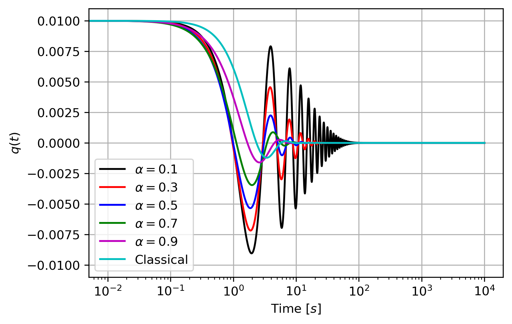
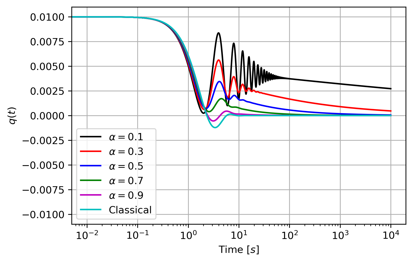
Figure 6: Anomalous linear free vibration modal displacement vs. time. (Left) Riemman-Liouville definition with short-time anomalies. (Right) Caputo definition with long-time anomalies.

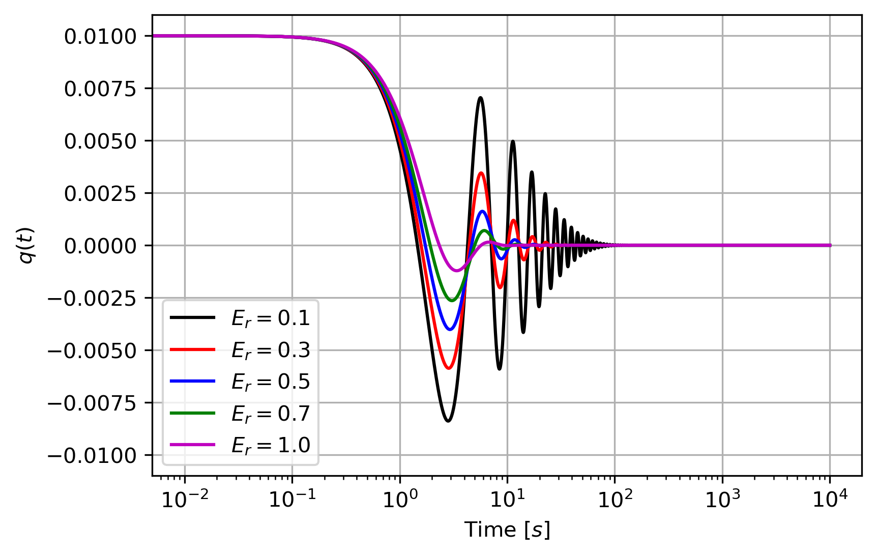
Figure 7: Classical linear free vibration modal displacement vs. time under varying values of $E_{r}$.

4 Perturbation Analysis of Nonlinear Equation

We use perturbation analysis to investigate the behavior of a nonlinear system, where we reduce a nonlinear fractional differential equation to an algebraic equation to solve for the steady state amplitude and phase of vibration.

4.1 Method of Multiple Scales

To investigate the dynamics of the system described by (30), we use the method of multiple scales [71, 72]. The new independent time scales and the integer-order derivative with respect to them are defined as

$$T_{m}=\epsilon^{m}\,t,\qquad D_{m}=\frac{\partial}{\partial T_{m}},\qquad m=0,1,2,\cdots.$$ (39)

It is also convenient to utilize another representation of the fractional derivative (see [73], Equation 5.82), which according to the Rieman-Liouville fractional derivative, is equivalent to the fractional power of the operator of conventional time-derivative, i.e. $\prescript{RL}{0}{\mathcal{D}}_{t}^{\alpha}=(\frac{d}{dt})^{\alpha}$. Therefore,

$$\frac{d}{dt} =D_{0}+\epsilon D_{1}+\cdots,\qquad\frac{d^{2}}{dt^{2}} =D^{2}_{0}+2\epsilon D_{0}D_{1}+\cdots,\qquad\prescript{RL}{0}{\mathcal{D}}_{t}^{\alpha} =(\frac{d}{dt})^{\alpha}=D^{\alpha}_{0}+\epsilon\alpha D^{\alpha-1}_{0}D_{1}+\cdots$$ (40)

The solution $q(t)$ can then be represented in terms of series expansion:

$$q(T_{0},T_{1},\cdots) =q_{0}(T_{0},T_{1},\cdots)+\epsilon q_{1}(T_{0},T_{1},\cdots)+\epsilon^{2}q_{2}(T_{0},T_{1},\cdots)+\cdots$$ (41)

We assume that the coefficients in the equation of motion have the following scaling

$$\frac{\mathcal{J}}{\mathcal{M}}=\epsilon\,m_{nl},\quad\frac{\mathcal{K}_{l}}{\mathcal{M}}=k_{l}=\omega^{2}_{0},\quad\frac{\mathcal{C}_{l}}{\mathcal{M}}=\epsilon\,c_{l},\quad\frac{\mathcal{K}_{nl}}{\mathcal{M}}=\epsilon\,k_{nl},\quad\frac{\mathcal{C}_{nl}}{\mathcal{M}}=\epsilon\,c_{nl},$$ (42)

and the base excitation $-\frac{\mathcal{M}_{b}}{\mathcal{M}}\,\ddot{{{v_{b}}}}$ is a harmonic function in the form $\epsilon\,F\cos(\Omega\,t)$. Thus, (30) can be expanded as

$$(D^{2}_{0}+2\epsilon D_{0}D_{1}+\cdots)(q_{0}+\epsilon q_{1}+\cdots)+\epsilon\,m_{nl}(D^{2}_{0}+2\epsilon D_{0}D_{1}+\cdots)(q_{0}+\epsilon q_{1}+\cdots)\,\times\,(q_{0}+\epsilon q_{1}+\cdots)^{2}$$

$$+ \epsilon\,m_{nl}(q_{0}+\epsilon q_{1}+\cdots)\times\,\left((D_{0}+\epsilon D_{1}+\cdots)(q_{0}+\epsilon q_{1}+\cdots)\right)^{2}+\omega^{2}_{0}\,(q_{0}+\epsilon q_{1}+\cdots)$$

$$+ \epsilon\,E_{r}\,c_{l}\,(D^{\alpha}_{0}+\epsilon\alpha D^{\alpha-1}_{0}D_{1}+\cdots)(q_{0}+\epsilon q_{1}+\cdots)+2\epsilon\,k_{nl}\,(q_{0}+\epsilon q_{1}+\cdots)^{3}$$

$$+ \frac{1}{2}\epsilon\,E_{r}\,c_{nl}\,(D^{\alpha}_{0}+\epsilon\alpha D^{\alpha-1}_{0}D_{1}+\cdots)(q_{0}+\epsilon q_{1}+\cdots)^{3}+\frac{3}{2}\epsilon\,E_{r}\,c_{nl}(q_{0}+\epsilon q_{1}+\cdots)^{2}$$

$$\left[(D^{\alpha}_{0}+\epsilon\alpha D^{\alpha-1}_{0}D_{1}+\cdots)(q_{0}+\epsilon q_{1}+\cdots)\right]=\epsilon\,F\cos(\Omega\,T_{0}).$$ (43)

By collecting similar coefficients of zero-th and first orders of $\epsilon$, we obtain the following equations

$$\mathcal{O}(\epsilon^{0}):D_{0}^{2}q_{0}+\omega_{0}^{2}q_{0}\,\,= \,\,0,$$ (44)

$$\mathcal{O}(\epsilon^{1}):D_{0}^{2}q_{1}+\omega_{0}^{2}q_{1}\,\,= \,\,-2D_{0}D_{1}q_{0}-m_{nl}\,\left(q_{0}^{2}D_{0}^{2}q_{0}+q_{0}(D_{0}q_{0})^{2}\right)-E_{r}\,c_{l}\,D^{\alpha}_{0}q_{0}-2\,k_{nl}\,q^{3}_{0}$$

$$-\frac{1}{2}\,E_{r}\,c_{nl}\,D^{\alpha}_{0}q^{3}_{0}-\frac{3}{2}\,E_{r}\,c_{nl}\,q^{2}_{0}D^{\alpha}_{0}q_{0}+F\cos(\Omega\,T_{0}).$$ (45)

The solution to (44) is of the form

$$q_{0}(T_{0},T_{1})=A(T_{1})\,e^{i\,\omega_{0}\,T_{0}}+c.c$$ (46)

where “c.c" denotes the complex conjugate. By substituting (46) into the right-hand-side of (45), we observe that different resonance cases are possible. In each case, we obtain the corresponding solvability conditions by removing the secular terms, i.e. the terms that grow in time unbounded. Then, we utilize the polar form $A=\frac{1}{2}a\,e^{i\,\varphi}$, where the real valued functions $a$ and $\varphi$ are the amplitude and phase lag of time response, respectively. Thus, the solution $q(t)$ becomes

$$q(t)=a(\epsilon\,t)\,\text{cos}(\omega_{0}\,t+\varphi(\epsilon\,t))+\mathcal{O}(\epsilon),$$ (47)

where the governing equations of $a$ and $\varphi$ are obtained by separating the real and imaginary parts.

4.1.1 Case 1: No Lumped Mass At The Tip

In this case, $M=J=0$, and thus, given the form (122) for the eigenfunctions $\phi(s)$ in D, the coefficients are computed as $\mathcal{M}=1$, $\mathcal{K}_{l}=\mathcal{C}_{l}=12.3624$, $\mathcal{M}_{b}=0.782992$, and $\mathcal{K}_{nl}=\mathcal{C}_{nl}=20.2203$. We consider the following cases:

$\bullet$ Free Vibration, $F=0$: Super Sensitivity to $\alpha$
In this case, the beam is not externally excited and thus, $F=0$. By removing the secular terms that are the coefficients of $e^{i\,\omega_{0}\,T_{0}}$ in the solvability condition, we find the governing equations of solution amplitude and phase as

$$\frac{da}{dT_{1}} =-E_{r}\,\omega_{0}^{\alpha-1}\sin(\alpha\frac{\pi}{2})\left(\frac{1}{2}\,c_{l}\,a+\frac{3}{8}\,c_{nl}\,a^{3}\right),$$ (48)

$$\frac{d\varphi}{dT_{1}} =\frac{1}{2}c_{l}\,E_{r}\,\omega_{0}^{\alpha-1}\,\cos\left(\frac{\pi\alpha}{2}\right)+\frac{3}{4}c_{nl}\,E_{r}\,\omega_{0}^{\alpha-1}\,\cos\left(\frac{\pi\alpha}{2}\right)\,a^{2}+\frac{3}{4}\,\omega_{0}^{-1}\,k_{nl}\,a^{2}.$$ (49)

We can see from the first equation (48) that the amplitude of free vibration decays out, where the decay rate $\tau_{d}=c_{l}\,E_{r}\,\omega_{0}^{\alpha-1}\sin(\alpha\frac{\pi}{2})$ directly depends on values of the fractional derivative $\alpha$ and the coefficients $E_{r}$ (see Fig. 8).

Figure 8: Nonlinear anomalous free vibration of a viscoelastic cantilever beam with no lumped mass at the tip and $E_{r}=0.1$. The rate of amplitude decay strongly depends on the fractional order $\alpha$, where a rapid decay is observed as $\alpha$ is increased (left). On the other hand, for increasing $\alpha$, the phase lag $\varphi(\epsilon t)$, increases in the lower range of $\alpha$, and decreases in the higher range of $\alpha$

We introduce the sensitivity index $S_{\tau_{d},\alpha}$ as the partial derivative of decay rate with respect to $\alpha$, i.e.

Figure 9: Anomalous super-sensitivity of the decay rate $\tau_{d}$ with respect to $\alpha$ under free vibration. Increasing $\alpha$ when $\alpha<\alpha_{cr}$ leads to higher dissipation and decay rate. The reverse effect is observed when $\alpha>\alpha_{cr}$. Here, the notions of softening/hardening are associated to high/lower decay rates as $\alpha$ is increased (introducing extra viscosity).

$$S_{\tau_{d},\alpha}=\frac{d\tau_{d}}{d\alpha}= \frac{\pi}{2}c_{l}\,E_{r}\,\omega_{0}^{\alpha-1}\,\cos(\alpha\frac{\pi}{2})+c_{l}\,E_{r}\,\omega_{0}^{\alpha-1}\sin(\alpha\frac{\pi}{2})\log(\omega_{0}).$$ (50)

The sensitivity index is computed and plotted in Fig. 9 for the same set of parameters as in Fig. 8. There exists a critical value

$$\alpha_{cr}=-\frac{2}{\pi}\tan^{-1}\left(\frac{\pi}{2\,\log(\omega_{0})}\right),$$ (51)

where $(dS_{\tau_{d},\alpha}/d\alpha)=0$. We observe in Fig.9 that by increasing $\alpha$ when $\alpha<\alpha_{cr}$, i.e. introducing more viscosity to the system, the dissipation rate, and thus decay rate, increases; this can be interpreted as a softening (stiffness-decreasing) region. Further increasing $\alpha$ when $\alpha>\alpha_{cr}$, will reversely results in decrease of decay rate; this can be interpreted as a hardening (more stiffening) region. We also note that $\alpha_{cr}$ solely depends on value of $\omega_{0}$, given in (42), and even though the value of $E_{r}$ affects decay rate, it does not change the value of $\alpha_{cr}$. Therefore, the region of super-sensitivity, where the anomalous transition between softening/hardening regimes takes place only depends on the standard natural frequency of the system.

Although the observed hardening response after a critical value of $\alpha$ in Fig.9 might seem counter-intuitive at first, we remark that here the notions of softening and hardening have a mixed nature regarding energy dissipation and time-scale dependent material stress response, which have anomalous nature for fractional viscoelasticity. Similar anomalous dynamics were also observed in ballistic, strain-driven yield stress responses of fractional visco-elasto-plastic truss structures [21]. In the following, we demonstrate two numerical tests by purely utilizing the constitutive response of the fractional Kelvin-Voigt model (19) to justify the observed behavior in Fig.9 by employing the tangent loss and the stress-strain response under monotone loads/relaxation.

Dissipation via tangent loss: By taking the Fourier transform of (19), we obtain the so-called complex modulus $G^{*}$ [52], which is given by:

$$G^{*}(\omega)=E_{\infty}+E_{\alpha}\omega^{\alpha}\left(\cos\left(\alpha\frac{\pi}{2}\right)+i\sin\left(\alpha\frac{\pi}{2}\right)\right),$$ (52)

from which the real and imaginary parts yield, respectively, the storage and loss moduli, as follows:

$$G^{\prime}(\omega)=E_{\infty}+E_{\alpha}\omega^{\alpha}\cos\left(\alpha\frac{\pi}{2}\right),\qquad G^{\prime\prime}(\omega)=E_{\alpha}\omega^{\alpha}\sin\left(\alpha\frac{\pi}{2}\right),$$

which represent, respectively, the stored and dissipated energies per cycle. Finally, we define the tangent loss, which represents the ratio between the dissipated/stored energies, and therefore related to the mechanical damping of the anomalous medium:

$$\tan\delta^{loss}=\frac{G^{\prime\prime}(\omega)}{G^{\prime}(\omega)}=\frac{E_{r}\omega^{\alpha}\sin\left(\alpha\frac{\pi}{2}\right)}{1+E_{r}\omega^{\alpha}\cos\left(\alpha\frac{\pi}{2}\right)}$$ (53)

We set $\omega=\omega_{0}$ and $E_{r}=1$ and demonstrate the results for (53) with varying fractional orders $\alpha$. We present the obtained results in Fig.10 (left), where we observe that increasing fractional orders lead to increased dissipation per loading cycle with the increase of the tangent loss, and the hardening part ($\alpha>\alpha_{c}$) is not associated with higher storage in the material. Instead, the increasing dissipation with $\alpha$ suggests an increasing damping of the mechanical structure.

Stress-time response for monotone loads/relaxation: In this test, we demonstrate how increasing fractional orders for the fractional model leads to increased hardening for sufficiently high strain rates. Therefore, we directly discretize (19) utilizing an L1-scheme [49] in a uniform time-grid and set $E_{\infty}=1$, $E_{\alpha}=1$. We also assume the following piecewise strain function: $\varepsilon(t)=(1/24)t$, for $0\leq t<2.5$ (monotone stress/strain), and $\varepsilon(t)=1/10$ for $2.5\leq t\leq 6$ (stress relaxation). The obtained results are illustrated in Fig.10 (right), where we observe that even for relatively low strain rates, there is a ballistic region nearby the initial time where higher fractional orders present higher values of stress, characterizing a rate-dependent stress-hardening response. However, due to the dissipative nature of fractional rheological elements, the initially higher-stress material softens after passing a critical point, due to its faster relaxation nature.

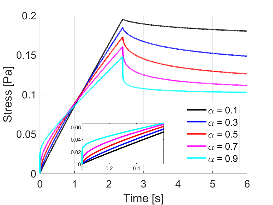
Figure 10: (Left) Storage and loss moduli, and tangent loss for the fractional Kelvin-Voigt model at $\omega_{0}$ with varying fractional-orders and $E_{r}=1$. (Right) Stress-time response under a monotone load with constant strain rate undergoing ballistic hardening response for short-time and higher $\alpha$, followed by a stress relaxation.

$\bullet$ Primary Resonance Case, $\Omega\approx\omega_{0}$
In the case of primary resonance, the excitation frequency is close to the natural frequency of the system. We let $\Omega=\omega_{0}+\epsilon\,\Delta$, where $\Delta$ is called the detuning parameter and thus, write the force function as $\frac{1}{2}F\,e^{i\,\Delta\,T_{1}}\,e^{i\,\omega_{0}\,T_{0}}+c.c$ . In this case, the force function also contributes to the secular terms. Therefore, we find the governing equations of solution amplitude and phase as

$$\frac{da}{dT_{1}}= -E_{r}\,\omega_{0}^{\alpha-1}\sin(\alpha\frac{\pi}{2})\left(\frac{1}{2}\,c_{l}\,a+\frac{3}{8}\,c_{nl}\,a^{3}\right)+\frac{1}{2}f\,\omega^{-1}_{0}\,\sin(\Delta T_{1}-\varphi),$$ (54)

$$a\,\frac{d\varphi}{dT_{1}}= \frac{1}{2}c_{l}\,E_{r}\,\omega_{0}^{\alpha-1}\,\cos(\frac{\pi\alpha}{2})\,a+\frac{3}{4}c_{nl}\,E_{r}\,\omega_{0}^{\alpha-1}\,\cos(\frac{\pi\alpha}{2})\,a^{3}+\frac{3}{4}\,\omega_{0}^{-1}\,k_{nl}\,a^{3}-\frac{1}{2}f\,\omega^{-1}_{0}\,\cos(\Delta T_{1}-\varphi),$$ (55)

in which the four parameters $\{\alpha,E_{r},f,\Delta\}$ mainly change the frequency response of the system. The equations (54) and (55) can be transformed into an autonomous system, where the $T_{1}$ does not appear explicitly, by letting

$$\gamma=\Delta\,T_{1}-\varphi.$$

The steady state solution occur when $\frac{da}{dT_{1}}=\frac{d\varphi}{dT_{1}}=0$, that gives

$$E_{r}\,\omega_{0}^{\alpha-1}\sin(\frac{\pi\alpha}{2})\left(\frac{c_{l}}{2}a+\frac{3c_{nl}}{8}a^{3}\right)=\frac{f}{2\,\omega_{0}}\sin(\gamma),$$ (56)

$$\left(\Delta-\frac{c_{l}}{2}E_{r}\,\omega_{0}^{\alpha-1}\,\cos(\frac{\pi\alpha}{2})\right)a-\frac{3}{4}\left(c_{nl}\,E_{r}\,\omega_{0}^{\alpha-1}\,\cos(\frac{\pi\alpha}{2})+\omega_{0}^{-1}\,k_{nl}\right)a^{3}=\frac{f}{2\,\omega_{0}}\cos(\gamma),$$ (57)

and thus, by squaring and adding these two equations, we get

$$\left[\frac{c_{l}}{2}E_{r}\,\omega_{0}^{\alpha-1}\sin(\frac{\pi\alpha}{2})\,a+\frac{3c_{nl}}{8}E_{r}\,\omega_{0}^{\alpha-1}\sin(\frac{\pi\alpha}{2})\,a^{3}\right]^{2}+\left[\left(\Delta-\frac{c_{l}}{2}E_{r}\,\omega_{0}^{\alpha-1}\,\cos(\frac{\pi\alpha}{2})\right)a\right.$$

$$\left.-\frac{3}{4}\left(c_{nl}\,E_{r}\,\omega_{0}^{\alpha-1}\,\cos(\frac{\pi\alpha}{2})+\omega_{0}^{-1}\,k_{nl}\right)a^{3}\right]^{2}=\frac{f^{2}}{4\,\omega^{2}_{0}}.$$ (58)

This can be written in a simpler way as

$$\left[A_{1}\,a+A_{2}\,a^{3}\right]^{2}+\left[B_{1}\,a+B_{2}\,a^{3}\right]^{2}=C,$$ (59)

where

$$A_{1}=\frac{c_{l}}{2}E_{r}\,\omega_{0}^{\alpha-1}\sin(\frac{\pi\alpha}{2}),\quad A_{2}=\frac{3c_{nl}}{8}E_{r}\,\omega_{0}^{\alpha-1}\sin(\frac{\pi\alpha}{2}),$$

$$B_{1}=\Delta-\frac{c_{l}}{2}E_{r}\,\omega_{0}^{\alpha-1}\,\cos(\frac{\pi\alpha}{2}),\quad B_{2}=-\frac{3}{4}\left(c_{nl}\,E_{r}\,\omega_{0}^{\alpha-1}\,\cos(\frac{\pi\alpha}{2})+\omega_{0}^{-1}\,k_{nl}\right),\quad C=\frac{f^{2}}{4\,\omega^{2}_{0}}.$$

Hence, the steady state response amplitude is the admissible root of

$$(A_{2}^{2}+B_{2}^{2})a^{6}+(2A_{1}A_{2}+2B_{1}B_{2})a^{4}+(A_{1}^{2}+B_{1}^{2})a^{2}-C=0,$$ (60)

which is a cubic equation in $a^{2}$. The discriminant of a cubic equation of the form $ax^{3}+bx^{2}+cx+d=0$ is given as $\vartheta=18abcd-4b^{3}d+b^{2}c^{2}-4ac^{3}-27a^{2}d^{2}$. The cubic equation (60) has one real root when $\vartheta<0$ and three distinct real roots when $\vartheta>0$. The main four parameters $\{\alpha,E_{r},f,\Delta\}$ dictate the value of coefficients $\{A_{1},A_{2},B_{1},B_{2},C\}$, the value of discriminant $\vartheta$, and thus the number of admissible steady state amplitudes. We see that for fixed values of $\{\alpha,E_{r},f\}$, by sweeping the detuning parameter $\Delta$ from lower to higher excitation frequency, the stable steady state amplitude bifurcates into two stable branches and one unstable branch, where they converge back to a stable amplitude by further increasing $\Delta$. Fig. 11 (left) shows the bifurcation diagram by sweeping the detuning parameter $\Delta$ and for different values of $\alpha$ when $E_{r}=0.3$ and $f=1$. The solid and dashed black lines are the stable and unstable amplitudes, respectively. The blue lines connect the bifurcation points (red dots) for each value of $\alpha$. We see that the bifurcation points are strongly related to the value of $\alpha$, meaning that by introducing extra viscosity to the system, i.e. increasing the value of $\alpha$, the amplitudes bifurcate and then converge back faster. Figure 11 (right) shows the frequency response of the system, i.e. the magnitude of steady state amplitudes versus excitation frequency. As the excitation frequency is swept to the right, the steady state amplitude increases, reaches a peak value, and then jumps down (see e.g. red dashed line for $\alpha=0.4$). The peak amplitude and the jump magnitude decreases as $\alpha$ is increased.

Figure 11: Primary resonance of the viscoelastic cantilever beam with no lumped mass at the tip. Steady state amplitude (right) and its bifurcation diagram (left) by changing the detuning parameter $\Delta$ for different values of $\alpha$ and $E_{r}=0.3,f=1$.

The coefficient $E_{r}=\frac{E_{\infty}}{E_{\alpha}}$ is the proportional contribution of fractional and pure elastic element. At a certain value while increasing this parameter, we see that the bifurcation disappears and the frequency response of system slightly changes. Fig. 12 shows the frequency response of the system for different values of $\{\alpha,E_{r}\}$ when $f=0.5$. In each sub-figure, we let $\alpha$ be fixed and then plot the frequency response for $E_{r}=\{0.1,0.2,\cdots,1\}$; the amplitude peak moves down as $E_{r}$ is increased. For higher values of $E_{r}$, we see that as $\alpha$ is increased, the amplitude peaks drift back to the left, showing a softening behavior in the system response.

Figure 12: Frequency-Response curve for the case of primary resonance in the viscoelastic cantilever beam with no lumped mass at the tip. Each sub-figure corresponds to a fixed value of $\alpha$ and $f$ when $E_{r}=\{0.1,0.2,\cdots,1\}$. As effect of fractional element becomes more pronounced, i.e. $\alpha$ and $E_{r}$ increase, the corresponding amplitude peaks decrease and shift towards the lower frequency range.

4.1.2 Case 2: Lumped Mass At The Tip

In this case, $M=J=1$, and thus, given the functions $\phi_{1}(x)$ in Appendix D, the coefficients are computed as $\mathcal{M}=1+70.769J+7.2734M$, $\mathcal{J}=5008.25$, $\mathcal{K}_{l}=\mathcal{C}_{l}=98.1058$, $\mathcal{M}_{b}=-0.648623-2.69692M$, and $\mathcal{K}_{nl}=\mathcal{C}_{nl}=2979.66$. Similar to Case 1, we consider the following cases:

$\bullet$ Free Vibration, $F=0$
Following the same steps as in Case 1, we see that the equation governing amplitude preserve its structure, but the governing equation of phase contains an extra term accommodating the $m_{nl}$.

$$\frac{da}{dT_{1}} =-E_{r}\,\omega_{0}^{\alpha-1}\sin(\alpha\frac{\pi}{2})\left(\frac{1}{2}\,c_{l}\,a+\frac{3}{8}\,c_{nl}\,a^{3}\right),$$ (61)

$$\frac{d\varphi}{dT_{1}}= \frac{1}{2}c_{l}\,E_{r}\,\omega_{0}^{\alpha-1}\,\cos\left(\frac{\pi\alpha}{2}\right)+\frac{3}{4}c_{nl}\,E_{r}\,\omega_{0}^{\alpha-1}\,\cos\left(\frac{\pi\alpha}{2}\right)\,a^{2}+\frac{3}{4}\,\omega_{0}^{-1}\,k_{nl}\,a^{2}-\frac{1}{4}\,m_{nl}\,\omega_{0}\,a^{2}.$$ (62)

This extra term does not significantly alter the behavior of phase and the whole system.

$\bullet$ Primary Resonance Case, $\Omega\approx\omega_{0}$
Similar to the free vibration, we see that the equation governing amplitude preserves its structure while the governing equation of phase contains an extra term accommodating the $m_{nl}$

$$\frac{da}{dT_{1}}= -E_{r}\,\omega_{0}^{\alpha-1}\sin(\alpha\frac{\pi}{2})\left(\frac{1}{2}\,c_{l}\,a+\frac{3}{8}\,c_{nl}\,a^{3}\right)+\frac{1}{2}f\,\omega^{-1}_{0}\,\sin(\Delta T_{1}-\varphi),$$ (63)

$$a\,\frac{d\varphi}{dT_{1}}= \frac{1}{2}c_{l}\,E_{r}\,\omega_{0}^{\alpha-1}\,\cos(\frac{\pi\alpha}{2})\,a+\frac{3}{4}c_{nl}\,E_{r}\,\omega_{0}^{\alpha-1}\,\cos(\frac{\pi\alpha}{2})\,a^{3}+\frac{3}{4}\,\omega_{0}^{-1}\,k_{nl}\,a^{3}-\frac{1}{2}f\,\omega^{-1}_{0}\,\cos(\Delta T_{1}-\varphi)-\frac{1}{4}\,m_{nl}\,\omega_{0}\,a^{3}.$$ (64)

Transforming the equations into an autonomous system by letting $\gamma=\Delta\,T_{1}-\varphi$, we obtain the governing equation of steady state solution as

$$\left[\frac{c_{l}}{2}E_{r}\,\omega_{0}^{\alpha-1}\sin(\frac{\pi\alpha}{2})\,a+\frac{3c_{nl}}{8}E_{r}\,\omega_{0}^{\alpha-1}\sin(\frac{\pi\alpha}{2})\,a^{3}\right]^{2}\left[\left(\Delta-\frac{c_{l}}{2}E_{r}\,\omega_{0}^{\alpha-1}\,\cos(\frac{\pi\alpha}{2})\right)a\right.$$

$$\left.-\frac{3}{4}\left(c_{nl}\,E_{r}\,\omega_{0}^{\alpha-1}\,\cos(\frac{\pi\alpha}{2})+\omega_{0}^{-1}\,k_{nl}+\frac{1}{3}\,m_{nl}\,\omega_{0}\right)a^{3}\right]^{2}=\frac{f^{2}}{4\,\omega^{2}_{0}},$$ (65)

which, similar to Case 1, can be written as

$$(A_{2}^{2}+B_{2}^{2})a^{6}+(2A_{1}A_{2}+2B_{1}B_{2})a^{4}+(A_{1}^{2}+B_{1}^{2})a^{2}-C=0,$$

where all the $A_{1}$, $A_{2}$, $B_{1}$, and $C$ are the same as in Case 1, but

$$B_{2}=-\frac{3}{4}\left(c_{nl}\,E_{r}\,\omega_{0}^{\alpha-1}\,\cos(\frac{\pi\alpha}{2})+\omega_{0}^{-1}\,k_{nl}+\frac{1}{3}\,m_{nl}\,\omega_{0}\right).$$

The corresponding cubic equation can be solved to obtain the bifurcation diagram and also the frequency response of the system. However, in addition to Case 1, we have an extra parameter $m_{nl}$ which affects the response of the system.

5 Summary and Discussion

In this work we investigated the anomalous nonlinear dynamics driven by the application of extraordinary materials. Our anomalous system is represented as a nonlinear fractional Kelvin-Voigt viscoelastic cantilever beam. A spectral method was employed for spatial discretization of the governing equation of motion, reducing it to a set of nonlinear fractional ODEs. The corresponding system was linearized and the time-fractional integration was carried out through a direct L1 finite-difference scheme, together with a Newmark method. For the nonlinear solution, a method of multiple scale was employed, and the time response of the beam subject to a base excitation was obtained. We performed a set of numerical experiments on the system response under varying fractional orders, representing different stages of material evolution, where we observed:

• Anomalous drift in peak amplitude response according to fractional orders, and the presence of a low-frequency critical point under linear forced vibration.

• Short-time and long-time anomalous behaviors under linear free vibration, respectively, for Riemann-Liouville and Caputo definitions.

• Super sensitivity of the amplitude response with respect to the fractional model parameters at free vibration.

• A critical behavior of the decay rate sensitivity with respect to $\alpha$, where increasing values of fractional order yielded higher decay rates (softening) before a critical value $\alpha_{cr}$. Lower decay rates (stress hardening) were observed beyond such critical value.

• A bifurcation behavior under steady-state amplitude at primary resonance case.

The choice of a fractional Kelvin-Voigt model in this work allowed us to describe a material in the intersection between anomalous and standard constitutive behavior, where the contribution of the SB element yields the power-law material response, while the Hookean spring reflects the instantaneous response of many engineering materials. In addition, the shifts in amplitude-frequency response with respect to the fractional order motivate future studies on the downscaling of fractional operators to the associated far-from-equilibrium dynamics (polymer caging/reptation, dislocation avalanches) in evolving heterogeneous microstructures [51]. In terms of modifications of the current model, different material distribution functions could be chosen, leading to application-based material design for a wide range of structural materials and anomalous systems, including microelectromechanical systems (MEMS). Finally, regarding numerical discretizations, one could utilize additional active vibration modes, as well as faster time-fractional integration methods, in order to better capture the fundamental dynamics of the presented system.

Appendix A Derivation of Governing Equation Using Extended Hamilton’s Principle

A.1 Equation of Motion

We recast the integral (20) as $\delta W=\int_{0}^{L}\int_{A}\sigma\,\delta\varepsilon\,dA\,\,ds$ for the considered cantilever beam, in which the variation of strain is $\delta\varepsilon=-\eta\,\delta\frac{\partial{\psi}}{\partial{s}}$, using (10). Therefore, by assuming the constitutive equation (19), the variation of total work is expressed as

$$\delta w =\int_{0}^{L}\int_{A}\left(-\eta\,E_{\infty}\,\frac{\partial{\psi}}{\partial{s}}-\eta\,E_{\alpha}\,\prescript{RL}{0}{\mathcal{D}}_{t}^{\alpha}\,\frac{\partial{\psi}}{\partial{s}}\right)\,(-\eta\,\delta\frac{\partial{\psi}}{\partial{s}})\,dA\,\,ds$$

$$=\int_{0}^{L}\left(E_{\infty}\,\left(\int_{A}\,\eta^{2}dA\right)\,\frac{\partial{\psi}}{\partial{s}}+E_{\alpha}\,\left(\int_{A}\,\eta^{2}dA\right)\,\prescript{RL}{0}{\mathcal{D}}_{t}^{\alpha}\,\frac{\partial{\psi}}{\partial{s}}\right)\,\delta\frac{\partial{\psi}}{\partial{s}}\,\,ds$$

$$=\int_{0}^{L}\left(E_{\infty}\,I\,\frac{\partial{\psi}}{\partial{s}}+E_{\alpha}\,I\,\prescript{RL}{0}{\mathcal{D}}_{t}^{\alpha}\,\frac{\partial{\psi}}{\partial{s}}\right)\,\delta\frac{\partial{\psi}}{\partial{s}}\,\,ds$$ (66)

where $I=\int_{A}\eta^{2}\,dA$. By approximation (9), we write the variation of curvature as

$$\delta\frac{\partial{\psi}}{\partial{s}}=(1+\frac{1}{2}(\frac{\partial{v}}{\partial{s}})^{2})\,\delta\frac{\partial^{2}{v}}{\partial{s}^{2}}+\frac{\partial^{2}{v}}{\partial{s}^{2}}\,\frac{\partial{v}}{\partial{s}}\,\delta\frac{\partial{v}}{\partial{s}}.$$ (67)

Therefore, the variation of total energy becomes

$$\delta w \!=\!\int_{0}^{L}\left(E_{\infty}I\frac{\partial^{2}{v}}{\partial{s}^{2}}(1+\frac{1}{2}(\frac{\partial{v}}{\partial{s}})^{2})+E_{\alpha}I\prescript{RL}{0}{\mathcal{D}}_{t}^{\alpha}\Big{[}\frac{\partial^{2}{v}}{\partial{s}^{2}}(1+\frac{1}{2}(\frac{\partial{v}}{\partial{s}})^{2})\Big{]}\right)(1+\frac{1}{2}(\frac{\partial{v}}{\partial{s}})^{2})\delta\frac{\partial^{2}{v}}{\partial{s}^{2}}\,\,ds$$

$$+\int_{0}^{L}\left(E_{\infty}I\frac{\partial^{2}{v}}{\partial{s}^{2}}(1+\frac{1}{2}(\frac{\partial{v}}{\partial{s}})^{2})+E_{\alpha}I\prescript{RL}{0}{\mathcal{D}}_{t}^{\alpha}\Big{[}\frac{\partial^{2}{v}}{\partial{s}^{2}}(1+\frac{1}{2}(\frac{\partial{v}}{\partial{s}})^{2})\Big{]}\right)\frac{\partial^{2}{v}}{\partial{s}^{2}}\frac{\partial{v}}{\partial{s}}\delta\frac{\partial{v}}{\partial{s}}\,\,ds$$ (68)

By expanding the terms and integrating by parts, we have

$$\delta w =\int_{0}^{L}\frac{\partial^{2}}{\partial{s}^{2}}\left(\left(E_{\infty}I\frac{\partial^{2}{v}}{\partial{s}^{2}}(1+\frac{1}{2}(\frac{\partial{v}}{\partial{s}})^{2})+E_{\alpha}I\prescript{RL}{0}{\mathcal{D}}_{t}^{\alpha}\Big{[}\frac{\partial^{2}{v}}{\partial{s}^{2}}(1+\frac{1}{2}(\frac{\partial{v}}{\partial{s}})^{2})\Big{]}\right)(1+\frac{1}{2}(\frac{\partial{v}}{\partial{s}})^{2})\right)\delta v\,\,ds$$

$$-\int_{0}^{L}\frac{\partial}{\partial{s}}\left(\left(E_{\infty}I\frac{\partial^{2}{v}}{\partial{s}^{2}}(1+\frac{1}{2}(\frac{\partial{v}}{\partial{s}})^{2})+E_{\alpha}I\prescript{RL}{0}{\mathcal{D}}_{t}^{\alpha}\Big{[}\frac{\partial^{2}{v}}{\partial{s}^{2}}(1+\frac{1}{2}(\frac{\partial{v}}{\partial{s}})^{2})\Big{]}\right)\frac{\partial^{2}{v}}{\partial{s}^{2}}\frac{\partial{v}}{\partial{s}}\right)\delta v\,\,ds$$

$$+\left(E_{\infty}I\frac{\partial^{2}{v}}{\partial{s}^{2}}(1+\frac{1}{2}(\frac{\partial{v}}{\partial{s}})^{2})+E_{\alpha}I\prescript{RL}{0}{\mathcal{D}}_{t}^{\alpha}\Big{[}\frac{\partial^{2}{v}}{\partial{s}^{2}}(1+\frac{1}{2}(\frac{\partial{v}}{\partial{s}})^{2})\Big{]}\right)(1+\frac{1}{2}(\frac{\partial{v}}{\partial{s}})^{2})\delta\frac{\partial{v}}{\partial{s}}\Bigg{|}_{0}^{L}$$

$$-\frac{\partial}{\partial{s}}\left(\left(E_{\infty}I\frac{\partial^{2}{v}}{\partial{s}^{2}}(1+\frac{1}{2}(\frac{\partial{v}}{\partial{s}})^{2})+E_{\alpha}I\prescript{RL}{0}{\mathcal{D}}_{t}^{\alpha}\Big{[}\frac{\partial^{2}{v}}{\partial{s}^{2}}(1+\frac{1}{2}(\frac{\partial{v}}{\partial{s}})^{2})\Big{]}\right)(1+\frac{1}{2}(\frac{\partial{v}}{\partial{s}})^{2})\right)\delta v\Bigg{|}_{0}^{L}$$

$$+\left(E_{\infty}I\frac{\partial^{2}{v}}{\partial{s}^{2}}(1+\frac{1}{2}(\frac{\partial{v}}{\partial{s}})^{2})+E_{\alpha}I\prescript{RL}{0}{\mathcal{D}}_{t}^{\alpha}\Big{[}\frac{\partial^{2}{v}}{\partial{s}^{2}}(1+\frac{1}{2}(\frac{\partial{v}}{\partial{s}})^{2})\Big{]}\right)\frac{\partial^{2}{v}}{\partial{s}^{2}}\frac{\partial{v}}{\partial{s}}\delta v\Bigg{|}_{0}^{L}$$ (69)

The prescribed geometry boundary conditions at the base of the beam, $s=0$, allow the variation of deflection and its first derivative to be zero at $s=0$, i.e. $\delta v(0,t)=\delta\frac{\partial{v}}{\partial{s}}(0,t)=0$. Therefore,

$$\delta w \!=\!\!\int_{0}^{L}\!\frac{\partial^{2}}{\partial{s}^{2}}\left(\left(E_{\infty}I\frac{\partial^{2}{v}}{\partial{s}^{2}}(1+\frac{1}{2}(\frac{\partial{v}}{\partial{s}})^{2})+E_{\alpha}I\prescript{RL}{0}{\mathcal{D}}_{t}^{\alpha}\Big{[}\frac{\partial^{2}{v}}{\partial{s}^{2}}(1+\frac{1}{2}(\frac{\partial{v}}{\partial{s}})^{2})\Big{]}\right)(1+\frac{1}{2}(\frac{\partial{v}}{\partial{s}})^{2})\right)\delta v\,\,ds$$

$$-\int_{0}^{L}\frac{\partial}{\partial{s}}\left(\left(E_{\infty}I\frac{\partial^{2}{v}}{\partial{s}^{2}}(1+\frac{1}{2}(\frac{\partial{v}}{\partial{s}})^{2})+E_{\alpha}I\prescript{RL}{0}{\mathcal{D}}_{t}^{\alpha}\Big{[}\frac{\partial^{2}{v}}{\partial{s}^{2}}(1+\frac{1}{2}(\frac{\partial{v}}{\partial{s}})^{2})\Big{]}\right)\frac{\partial^{2}{v}}{\partial{s}^{2}}\frac{\partial{v}}{\partial{s}}\right)\delta v\,\,ds$$

$$+\left(E_{\infty}I\frac{\partial^{2}{v}}{\partial{s}^{2}}(1+\frac{1}{2}(\frac{\partial{v}}{\partial{s}})^{2})\!+\!E_{\alpha}I\prescript{RL}{0}{\mathcal{D}}_{t}^{\alpha}\Big{[}\frac{\partial^{2}{v}}{\partial{s}^{2}}(1\!+\!\frac{1}{2}(\frac{\partial{v}}{\partial{s}})^{2})\Big{]}\right)(1\!+\!\frac{1}{2}(\frac{\partial{v}}{\partial{s}})^{2})\Bigg{|}_{s=L}\delta\frac{\partial{v}}{\partial{s}}(L,t)$$

$$-\frac{\partial}{\partial{s}}\left(\left(E_{\infty}I\frac{\partial^{2}{v}}{\partial{s}^{2}}(1+\frac{1}{2}(\frac{\partial{v}}{\partial{s}})^{2})\!+\!E_{\alpha}I\prescript{RL}{0}{\mathcal{D}}_{t}^{\alpha}\Big{[}\frac{\partial^{2}{v}}{\partial{s}^{2}}(1\!+\!\frac{1}{2}(\frac{\partial{v}}{\partial{s}})^{2})\Big{]}\right)(1\!+\!\frac{1}{2}(\frac{\partial{v}}{\partial{s}})^{2})\right)\Bigg{|}_{s=L}\delta v(L,t)$$

$$+\left(E_{\infty}I\frac{\partial^{2}{v}}{\partial{s}^{2}}(1+\frac{1}{2}(\frac{\partial{v}}{\partial{s}})^{2})+E_{\alpha}I\prescript{RL}{0}{\mathcal{D}}_{t}^{\alpha}\Big{[}\frac{\partial^{2}{v}}{\partial{s}^{2}}(1+\frac{1}{2}(\frac{\partial{v}}{\partial{s}})^{2}\Big{]}\right)\frac{\partial^{2}{v}}{\partial{s}^{2}}\frac{\partial{v}}{\partial{s}}\Bigg{|}_{s=L}\delta v(L,t)$$ (70)

Let $\varrho$ be mass per unit volume of the beam, $M$ and $J$ be the mass and rotatory inertia of the lumped mass at the tip of beam. By considering the displacement and velocity of the beam given in (2) and (3), respectively, the kinetic energy is obtained as

$$T= \frac{1}{2}\,\int_{0}^{L}\int_{A}\varrho\,(\frac{\partial{\textbf{r}}}{\partial{t}})^{2}\,dA\,ds+\frac{1}{2}M\left((\frac{\partial{u}}{\partial{t}})^{2}+(\frac{\partial{v}}{\partial{t}}+\dot{{v_{b}}})^{2}\right)\Big{|}_{s=L}+\frac{1}{2}J(\frac{\partial{\psi}}{\partial{t}})^{2}\Big{|}_{s=L},$$

$$= \frac{1}{2}\,\int_{0}^{L}\int_{A}\varrho\,\Big{\{}(\frac{\partial{u}}{\partial{t}}-\eta\,\frac{\partial{\psi}}{\partial{t}}\,\cos(\psi))^{2}+(\frac{\partial{v}}{\partial{t}}+\dot{{v_{b}}}-\eta\,\frac{\partial{\psi}}{\partial{t}}\,\sin(\psi))^{2}\Big{\}}\,dA\,ds+\frac{1}{2}M\left((\frac{\partial{u}}{\partial{t}})^{2}+(\frac{\partial{v}}{\partial{t}}+\dot{{v_{b}}})^{2}\right)\Big{|}_{s=L}+\frac{1}{2}J(\frac{\partial{\psi}}{\partial{t}})^{2}\Big{|}_{s=L},$$

$$= \frac{1}{2}\,\int_{0}^{L}\int_{A}\varrho\,\Big{\{}(\frac{\partial{u}}{\partial{t}})^{2}-2\eta\,\frac{\partial{u}}{\partial{t}}\,\frac{\partial{\psi}}{\partial{t}}\,\cos(\psi)+\eta^{2}\,(\frac{\partial{\psi}}{\partial{t}})^{2}\,\cos^{2}(\psi)+(\frac{\partial{v}}{\partial{t}})^{2}+{\dot{{v_{b}}}}^{2}+2\frac{\partial{v}}{\partial{t}}\,\dot{{v_{b}}}$$

$$-2\eta\,(\frac{\partial{v}}{\partial{t}}\!+\!\dot{{v_{b}}})\frac{\partial{\psi}}{\partial{t}}\,\sin(\psi)\!+\!\eta^{2}(\frac{\partial{\psi}}{\partial{t}})^{2}\,\sin^{2}(\psi)\Big{\}}dAds+\frac{1}{2}M\left((\frac{\partial{u}}{\partial{t}})^{2}+(\frac{\partial{v}}{\partial{t}}+\dot{{v_{b}}})^{2}\right)\Big{|}_{s=L}+\frac{1}{2}J(\frac{\partial{\psi}}{\partial{t}})^{2}\Big{|}_{s=L},$$

$$= \frac{1}{2}\,\int_{0}^{L}\int_{A}\varrho\,\Big{\{}(\frac{\partial{u}}{\partial{t}})^{2}+(\frac{\partial{v}}{\partial{t}})^{2}+{\dot{{v_{b}}}}^{2}+2\frac{\partial{v}}{\partial{t}}\,\dot{{v_{b}}}-2\eta\,\frac{\partial{u}}{\partial{t}}\,\frac{\partial{\psi}}{\partial{t}}\,\cos(\psi)+\eta^{2}\,(\frac{\partial{\psi}}{\partial{t}})^{2}-2\eta\,(\frac{\partial{v}}{\partial{t}}+\dot{{v_{b}}})\frac{\partial{\psi}}{\partial{t}}\,\sin(\psi)\Big{\}}\,dA\,ds$$

$$+\frac{1}{2}M\left((\frac{\partial{u}}{\partial{t}})^{2}+(\frac{\partial{v}}{\partial{t}}+\dot{{v_{b}}})^{2}\right)\Big{|}_{s=L}+\frac{1}{2}J(\frac{\partial{\psi}}{\partial{t}})^{2}\Big{|}_{s=L}.$$ (71)

Let

$$\rho=\int_{A}\varrho dA,\quad\mathcal{J}_{1}=\int_{A}\varrho\,\eta\,dA,\quad\mathcal{J}_{2}=\int_{A}\varrho\,\eta^{2}dA.$$

$\rho$ is the mass per unit length of the beam, $\mathcal{J}_{1}$ is the first moment of inertia and is zero because the reference point of coordinate system attached to the cross section coincides with the mass centroid, and $\mathcal{J}_{2}$ is the second moment of inertia, which is very small for slender beam and can be ignored [63]. Assuming that the velocity along the length of the beam, $\dot{u}$, is relatively small compared to the lateral velocity $\dot{v}+\dot{{v_{b}}}$, the kinetic energy of the beam can be reduced to

$$T= \frac{1}{2}\,\rho\int_{0}^{L}(\frac{\partial{v}}{\partial{t}}+\dot{{v_{b}}})^{2}\,ds+\frac{1}{2}M(\frac{\partial{v}}{\partial{t}}+\dot{{v_{b}}})^{2}\Big{|}_{s=L}+\frac{1}{2}J(\frac{\partial{\psi}}{\partial{t}})^{2}\Big{|}_{s=L},$$ (72)

where its variation can be taken as

$$\delta T= \rho\int_{0}^{L}(\frac{\partial{v}}{\partial{t}}+\dot{{{v_{b}}}})\,\delta\frac{\partial{v}}{\partial{t}}\,ds+M(\frac{\partial{v}}{\partial{t}}+\dot{{{v_{b}}}})\,\delta\frac{\partial{v}}{\partial{t}}\Big{|}_{s=L}+J\frac{\partial{\psi}}{\partial{t}}\,\delta\frac{\partial{\psi}}{\partial{t}}\Big{|}_{s=L},$$ (73)

in which $\frac{\partial{\psi}}{\partial{t}}$ is given in (8) and $\delta\frac{\partial{\psi}}{\partial{t}}$ can be obtained as

$$\delta\frac{\partial{\psi}}{\partial{t}}\simeq(1+\frac{1}{2}(\frac{\partial{v}}{\partial{s}})^{2})\delta\frac{\partial^{2}{v}}{\partial{t}\partial{s}}+\frac{\partial{v}}{\partial{s}}\frac{\partial^{2}{v}}{\partial{t}\partial{s}}\delta\frac{\partial{v}}{\partial{s}}.$$

Therefore,

$$\delta T\simeq \rho\int_{0}^{L}(\frac{\partial{v}}{\partial{t}}+\dot{{{v_{b}}}})\delta\frac{\partial{v}}{\partial{t}}ds+M(\frac{\partial{v}}{\partial{t}}+\dot{{{v_{b}}}})\delta\frac{\partial{v}}{\partial{t}}\Big{|}_{s=L}\!+\!J\left(\frac{\partial^{2}{v}}{\partial{t}\partial{s}}(1\!+\!(\frac{\partial{v}}{\partial{s}})^{2})\delta\frac{\partial^{2}{v}}{\partial{t}\partial{s}}\!+\!\frac{\partial{v}}{\partial{s}}(\frac{\partial^{2}{v}}{\partial{t}\partial{s}})^{2}\delta\frac{\partial{v}}{\partial{s}}\right)\Big{|}_{s=L}.$$ (74)

The time integration of $\delta T$ takes the following form through integration by parts

$$\int_{t_{1}}^{t_{2}}\delta T\,dt= \int_{t_{1}}^{t_{2}}\Bigg{\{}\rho\int_{0}^{L}(\frac{\partial{v}}{\partial{t}}+\dot{{{v_{b}}}})\,\delta\frac{\partial{v}}{\partial{t}}\,ds\!+\!M(\frac{\partial{v}}{\partial{t}}+\dot{{{v_{b}}}})\,\delta\frac{\partial{v}}{\partial{t}}\Big{|}_{s=L}+J\left(\frac{\partial^{2}{v}}{\partial{t}\partial{s}}(1+(\frac{\partial{v}}{\partial{s}})^{2})\delta\frac{\partial^{2}{v}}{\partial{t}\partial{s}}+\frac{\partial{v}}{\partial{s}}(\frac{\partial^{2}{v}}{\partial{t}\partial{s}})^{2}\delta\frac{\partial{v}}{\partial{s}}\right)\Big{|}_{s=L}\Bigg{\}}\,dt$$

$$= \int_{t_{1}}^{t_{2}}\rho\int_{0}^{L}(\frac{\partial{v}}{\partial{t}}\!+\!\dot{{{v_{b}}}})\,\delta\frac{\partial{v}}{\partial{t}}\,ds\,dt\!+\!\!M\!\int_{t_{1}}^{t_{2}}(\frac{\partial{v}}{\partial{t}}\!+\!\dot{{{v_{b}}}})\,\delta\frac{\partial{v}}{\partial{t}}\Big{|}_{s=L}\,dt\!+\!\!J\!\int_{t_{1}}^{t_{2}}\left(\frac{\partial^{2}{v}}{\partial{t}\partial{s}}(1+(\frac{\partial{v}}{\partial{s}})^{2})\delta\frac{\partial^{2}{v}}{\partial{t}\partial{s}}+\frac{\partial{v}}{\partial{s}}(\frac{\partial^{2}{v}}{\partial{t}\partial{s}})^{2}\delta\frac{\partial{v}}{\partial{s}}\right)\Big{|}_{s=L}\,dt$$

$$= \rho\int_{0}^{L}\int_{t_{1}}^{t_{2}}(\frac{\partial{v}}{\partial{t}}+\dot{{{v_{b}}}})\,\delta\frac{\partial{v}}{\partial{t}}\,dt\,ds+M\int_{t_{1}}^{t_{2}}(\frac{\partial{v}}{\partial{t}}+\dot{{{v_{b}}}})\,\delta\frac{\partial{v}}{\partial{t}}\,dt\,\Big{|}_{s=L}\!+\!J\int_{t_{1}}^{t_{2}}\left(\frac{\partial^{2}{v}}{\partial{t}\partial{s}}(1+(\frac{\partial{v}}{\partial{s}})^{2})\delta\frac{\partial^{2}{v}}{\partial{t}\partial{s}}+\frac{\partial{v}}{\partial{s}}(\frac{\partial^{2}{v}}{\partial{t}\partial{s}})^{2}\delta\frac{\partial{v}}{\partial{s}}\right)\,dt\,\Big{|}_{s=L}$$

$$= \rho\!\int_{0}^{L}\!\left[(\frac{\partial{v}}{\partial{t}}\!+\!\dot{{{v_{b}}}})\delta{v}\Big{|}_{t_{1}}^{t_{2}}\!-\!\!\int_{t_{1}}^{t_{2}}\!(\frac{\partial^{2}{v}}{\partial{t}^{2}}\!+\!\ddot{{{v_{b}}}})\delta{v}dt\right]ds\!+\!M(\frac{\partial{v}}{\partial{t}}\!+\!\dot{{{v_{b}}}})\delta v\Big{|}_{s=L}\Big{|}_{t_{1}}^{t_{2}}\!-\!M\!\int_{t_{1}}^{t_{2}}(\frac{\partial^{2}{v}}{\partial{t}^{2}}\!+\!\ddot{{{v_{b}}}})\delta vdt\Big{|}_{s=L}$$

$$\!+\!J\frac{\partial^{2}{v}}{\partial{t}\partial{s}}(1\!+\!(\frac{\partial{v}}{\partial{s}})^{2})\delta\frac{\partial{v}}{\partial{s}}\Big{|}_{s=L}\Big{|}_{t_{1}}^{t_{2}}\!-\!J\int_{t_{1}}^{t_{2}}\left(\frac{\partial^{3}{v}}{\partial{t}^{2}\partial{s}}(1\!+\!(\frac{\partial{v}}{\partial{s}})^{2})\!+\!\frac{\partial{v}}{\partial{s}}(\frac{\partial^{2}{v}}{\partial{t}\partial{s}})^{2}\right)\delta\frac{\partial{v}}{\partial{s}}dt\Big{|}_{s=L}$$

$$\!=\! -\!\int_{t_{1}}^{t_{2}}\!\Bigg{\{}\rho\int_{0}^{L}(\frac{\partial^{2}{v}}{\partial{t}^{2}}\!+\!\ddot{{{v_{b}}}})\delta{v}ds\!+\!M(\frac{\partial^{2}{v}}{\partial{t}^{2}}\!+\!\ddot{{{v_{b}}}})\delta v\Big{|}_{s=L}+J\left(\frac{\partial^{3}{v}}{\partial{t}^{2}\partial{s}}(1\!+\!(\frac{\partial{v}}{\partial{s}})^{2})\!+\!\frac{\partial{v}}{\partial{s}}(\frac{\partial^{2}{v}}{\partial{t}\partial{s}})^{2}\right)\delta\frac{\partial{v}}{\partial{s}}\Big{|}_{s=L}\Bigg{\}}dt,$$ (75)

where we consider that $\delta v=\delta\frac{\partial{v}}{\partial{s}}=0$ at $t=t_{1}$ and $t=t_{2}$. Therefore, the extended Hamilton’s principle takes the form

$$\int_{t_{1}}^{t_{2}}\Bigg{\{}\int_{0}^{L}\Bigg{[}-\rho(\frac{\partial^{2}{v}}{\partial{t}^{2}}+\ddot{{{v_{b}}}})-\frac{\partial^{2}}{\partial{s}^{2}}\left(\left(E_{\infty}\,I\,\frac{\partial^{2}{v}}{\partial{s}^{2}}(1+\frac{1}{2}(\frac{\partial{v}}{\partial{s}})^{2})+E_{\alpha}\,I\,\prescript{RL}{0}{\mathcal{D}}_{t}^{\alpha}\,\Big{[}\frac{\partial^{2}{v}}{\partial{s}^{2}}(1+\frac{1}{2}(\frac{\partial{v}}{\partial{s}})^{2})\Big{]}\right)(1+\frac{1}{2}(\frac{\partial{v}}{\partial{s}})^{2})\right)$$

$$+\frac{\partial}{\partial{s}}\left(\left(E_{\infty}\,I\,\frac{\partial^{2}{v}}{\partial{s}^{2}}(1+\frac{1}{2}(\frac{\partial{v}}{\partial{s}})^{2})+E_{\alpha}\,I\,\prescript{RL}{0}{\mathcal{D}}_{t}^{\alpha}\,\Big{[}\frac{\partial^{2}{v}}{\partial{s}^{2}}(1+\frac{1}{2}(\frac{\partial{v}}{\partial{s}})^{2})\Big{]}\right)\frac{\partial^{2}{v}}{\partial{s}^{2}}\,\frac{\partial{v}}{\partial{s}}\,\right)\Bigg{]}\,\delta{v}\,ds-M(\frac{\partial^{2}{v}}{\partial{t}^{2}}+\ddot{{{v_{b}}}})\Big{|}_{s=L}\,\delta v(L,t)$$

$$\!-\!J\left(\frac{\partial^{3}{v}}{\partial{t}^{2}\partial{s}}(1\!+\!(\frac{\partial{v}}{\partial{s}})^{2})\!+\!\frac{\partial{v}}{\partial{s}}(\frac{\partial^{2}{v}}{\partial{t}\partial{s}})^{2}\right)\Big{|}_{s=L}\,\delta\frac{\partial{v}}{\partial{s}}(L,t)\!-\!\left(E_{\infty}\,I\,\frac{\partial^{2}{v}}{\partial{s}^{2}}(1\!+\!\frac{1}{2}(\frac{\partial{v}}{\partial{s}})^{2})\!+\!E_{\alpha}I\prescript{RL}{0}{\mathcal{D}}_{t}^{\alpha}\Big{[}\frac{\partial^{2}{v}}{\partial{s}^{2}}(1\!+\!\frac{1}{2}(\frac{\partial{v}}{\partial{s}})^{2})\Big{]}\right)(1\!+\!\frac{1}{2}(\frac{\partial{v}}{\partial{s}})^{2})\Bigg{|}_{s=L}\delta\frac{\partial{v}}{\partial{s}}(L,t)$$

$$+\frac{\partial}{\partial{s}}\left(\left(E_{\infty}\,I\,\frac{\partial^{2}{v}}{\partial{s}^{2}}(1+\frac{1}{2}(\frac{\partial{v}}{\partial{s}})^{2})+E_{\alpha}I\prescript{RL}{0}{\mathcal{D}}_{t}^{\alpha}\Big{[}\frac{\partial^{2}{v}}{\partial{s}^{2}}(1\!+\!\frac{1}{2}(\frac{\partial{v}}{\partial{s}})^{2})\Big{]}\right)(1\!+\!\frac{1}{2}(\frac{\partial{v}}{\partial{s}})^{2})\right)\Bigg{|}_{s=L}\delta v(L,t)$$

$$-\left(E_{\infty}\,I\,\frac{\partial^{2}{v}}{\partial{s}^{2}}(1+\frac{1}{2}(\frac{\partial{v}}{\partial{s}})^{2})+E_{\alpha}I\prescript{RL}{0}{\mathcal{D}}_{t}^{\alpha}\Big{[}\frac{\partial^{2}{v}}{\partial{s}^{2}}(1\!+\!\frac{1}{2}(\frac{\partial{v}}{\partial{s}})^{2})\Big{]}\right)\frac{\partial^{2}{v}}{\partial{s}^{2}}\frac{\partial{v}}{\partial{s}}\Bigg{|}_{s=L}\delta v(L,t)\Bigg{\}}dt\!=\!0$$ (76)

Invoking the arbitrariness of virtual displacement $\delta v$, we obtain the strong form of the equation of motion as:

$$\rho\,\frac{\partial^{2}{v}}{\partial{t}^{2}}+E_{\infty}\,I\,\frac{\partial^{2}}{\partial{s}^{2}}\left(\frac{\partial^{2}{v}}{\partial{s}^{2}}(1+\frac{1}{2}(\frac{\partial{v}}{\partial{s}})^{2})^{2}\right)+E_{\alpha}\,I\,\frac{\partial^{2}}{\partial{s}^{2}}\left((1+\frac{1}{2}(\frac{\partial{v}}{\partial{s}})^{2})\,\prescript{RL}{0}{\mathcal{D}}_{t}^{\alpha}\,\Big{[}\frac{\partial^{2}{v}}{\partial{s}^{2}}(1+\frac{1}{2}(\frac{\partial{v}}{\partial{s}})^{2})\Big{]}\right)$$

$$-E_{\infty}\,I\,\frac{\partial}{\partial{s}}\left(\frac{\partial{v}}{\partial{s}}\,(\frac{\partial^{2}{v}}{\partial{s}^{2}})^{2}(1+\frac{1}{2}(\frac{\partial{v}}{\partial{s}})^{2})\right)-E_{\alpha}\,I\,\frac{\partial}{\partial{s}}\left(\frac{\partial{v}}{\partial{s}}\,\frac{\partial^{2}{v}}{\partial{s}^{2}}\,\prescript{RL}{0}{\mathcal{D}}_{t}^{\alpha}\,\Big{[}\frac{\partial^{2}{v}}{\partial{s}^{2}}(1+\frac{1}{2}(\frac{\partial{v}}{\partial{s}})^{2})\Big{]}\right)=-\rho\,\ddot{{{v_{b}}}},$$ (77)

which is subject to the following natural boundary conditions:

$$J\left(\frac{\partial^{3}{v}}{\partial{t}^{2}\partial{s}}(1+(\frac{\partial{v}}{\partial{s}})^{2})+\frac{\partial{v}}{\partial{s}}(\frac{\partial^{2}{v}}{\partial{t}\partial{s}})^{2}\right)+E_{\infty}\,I\,\frac{\partial^{2}{v}}{\partial{s}^{2}}(1+\frac{1}{2}(\frac{\partial{v}}{\partial{s}})^{2})^{2}+E_{\alpha}\,I\,(1+\frac{1}{2}(\frac{\partial{v}}{\partial{s}})^{2})\,\prescript{RL}{0}{\mathcal{D}}_{t}^{\alpha}\,\Big{[}\frac{\partial^{2}{v}}{\partial{s}^{2}}(1+\frac{1}{2}(\frac{\partial{v}}{\partial{s}})^{2})\Big{]}\,\,\Bigg{|}_{s=L}=0,$$

$$M(\frac{\partial^{2}{v}}{\partial{t}^{2}}+\ddot{{{v_{b}}}})-\frac{\partial}{\partial{s}}\left(E_{\infty}\,I\,\frac{\partial^{2}{v}}{\partial{s}^{2}}(1+\frac{1}{2}(\frac{\partial{v}}{\partial{s}})^{2})^{2}+E_{\alpha}\,I\,(1+\frac{1}{2}(\frac{\partial{v}}{\partial{s}})^{2})\,\prescript{RL}{0}{\mathcal{D}}_{t}^{\alpha}\,\Big{[}\frac{\partial^{2}{v}}{\partial{s}^{2}}(1+\frac{1}{2}(\frac{\partial{v}}{\partial{s}})^{2})\Big{]}\right)$$

$$+\left(E_{\infty}\,I\,\frac{\partial{v}}{\partial{s}}\,(\frac{\partial^{2}{v}}{\partial{s}^{2}})^{2}(1+\frac{1}{2}(\frac{\partial{v}}{\partial{s}})^{2})+E_{\alpha}\,I\,\frac{\partial{v}}{\partial{s}}\,\frac{\partial^{2}{v}}{\partial{s}^{2}}\,\prescript{RL}{0}{\mathcal{D}}_{t}^{\alpha}\,\Big{[}\frac{\partial^{2}{v}}{\partial{s}^{2}}(1+\frac{1}{2}(\frac{\partial{v}}{\partial{s}})^{2})\Big{]}\right)\,\,\Bigg{|}_{s=L}=0.$$ (78)

Following a similar approach as in (9) in deriving the beam curvature, we obtain the approximations below, where we only consider up to third order terms and remove the higher order terms (HOTs).

$$\frac{\partial^{2}{v}}{\partial{s}^{2}}(1+\frac{1}{2}(\frac{\partial{v}}{\partial{s}})^{2})^{2}=\frac{\partial^{2}{v}}{\partial{s}^{2}}+\frac{\partial^{2}{v}}{\partial{s}^{2}}(\frac{\partial{v}}{\partial{s}})^{2}+\text{HOTs}$$

$$(1+\frac{1}{2}(\frac{\partial{v}}{\partial{s}})^{2})\,\prescript{RL}{0}{\mathcal{D}}_{t}^{\alpha}\,\Big{[}\frac{\partial^{2}{v}}{\partial{s}^{2}}(1+\frac{1}{2}(\frac{\partial{v}}{\partial{s}})^{2})\Big{]}=\prescript{RL}{0}{\mathcal{D}}_{t}^{\alpha}\Big{[}\frac{\partial^{2}{v}}{\partial{s}^{2}}(1\!+\!\frac{1}{2}(\frac{\partial{v}}{\partial{s}})^{2})\Big{]}\!+\!\frac{1}{2}(\frac{\partial{v}}{\partial{s}})^{2}\prescript{RL}{0}{\mathcal{D}}_{t}^{\alpha}\frac{\partial^{2}{v}}{\partial{s}^{2}}\!+\!\text{HOTs}$$

$$\frac{\partial{v}}{\partial{s}}\,(\frac{\partial^{2}{v}}{\partial{s}^{2}})^{2}(1+\frac{1}{2}(\frac{\partial{v}}{\partial{s}})^{2})=\frac{\partial{v}}{\partial{s}}\,(\frac{\partial^{2}{v}}{\partial{s}^{2}})^{2}+\text{HOTs}$$

$$\frac{\partial{v}}{\partial{s}}\,\frac{\partial^{2}{v}}{\partial{s}^{2}}\,\prescript{RL}{0}{\mathcal{D}}_{t}^{\alpha}\,\Big{[}\frac{\partial^{2}{v}}{\partial{s}^{2}}(1+\frac{1}{2}(\frac{\partial{v}}{\partial{s}})^{2})\Big{]}=\frac{\partial{v}}{\partial{s}}\,\frac{\partial^{2}{v}}{\partial{s}^{2}}\,\prescript{RL}{0}{\mathcal{D}}_{t}^{\alpha}\,\frac{\partial^{2}{v}}{\partial{s}^{2}}+\text{HOTs}$$

Therefore, the strong form can be approximated up to the third order and the problem then reads as: find $v\in V$ such that

$$m\,\frac{\partial^{2}{v}}{\partial{t}^{2}}+\frac{\partial^{2}}{\partial{s}^{2}}\left(\frac{\partial^{2}{v}}{\partial{s}^{2}}+\frac{\partial^{2}{v}}{\partial{s}^{2}}(\frac{\partial{v}}{\partial{s}})^{2}\right)-\frac{\partial}{\partial{s}}\left(\frac{\partial{v}}{\partial{s}}\,(\frac{\partial^{2}{v}}{\partial{s}^{2}})^{2}\right)+E_{r}\frac{\partial^{2}}{\partial{s}^{2}}\left(\prescript{RL}{0}{\mathcal{D}}_{t}^{\alpha}\Big{[}\frac{\partial^{2}{v}}{\partial{s}^{2}}(1+\frac{1}{2}(\frac{\partial{v}}{\partial{s}})^{2})\Big{]}+\frac{1}{2}(\frac{\partial{v}}{\partial{s}})^{2}\prescript{RL}{0}{\mathcal{D}}_{t}^{\alpha}\frac{\partial^{2}{v}}{\partial{s}^{2}}\right)$$

$$-E_{r}\frac{\partial}{\partial{s}}\left(\frac{\partial{v}}{\partial{s}}\frac{\partial^{2}{v}}{\partial{s}^{2}}\prescript{RL}{0}{\mathcal{D}}_{t}^{\alpha}\frac{\partial^{2}{v}}{\partial{s}^{2}}\right)=-m\ddot{{{v_{b}}}},$$ (79)

By rearranging

$$m\,\frac{\partial^{2}{v}}{\partial{t}^{2}}+\frac{\partial^{2}}{\partial{s}^{2}}\left(\frac{\partial^{2}{v}}{\partial{s}^{2}}+\frac{\partial^{2}{v}}{\partial{s}^{2}}(\frac{\partial{v}}{\partial{s}})^{2}+E_{r}\prescript{RL}{0}{\mathcal{D}}_{t}^{\alpha}\,\Big{[}\frac{\partial^{2}{v}}{\partial{s}^{2}}(1+\frac{1}{2}(\frac{\partial{v}}{\partial{s}})^{2})\Big{]}+\frac{1}{2}E_{r}(\frac{\partial{v}}{\partial{s}})^{2}\,\prescript{RL}{0}{\mathcal{D}}_{t}^{\alpha}\,\frac{\partial^{2}{v}}{\partial{s}^{2}}\right)$$

$$-\frac{\partial}{\partial{s}}\left(\frac{\partial{v}}{\partial{s}}\,(\frac{\partial^{2}{v}}{\partial{s}^{2}})^{2}+E_{r}\frac{\partial{v}}{\partial{s}}\,\frac{\partial^{2}{v}}{\partial{s}^{2}}\,\prescript{RL}{0}{\mathcal{D}}_{t}^{\alpha}\,\frac{\partial^{2}{v}}{\partial{s}^{2}}\right)=-m\,\ddot{{{v_{b}}}},$$ (80)

subject to the following boundary conditions:

$$v\Big{|}_{s=0}=\frac{\partial{v}}{\partial{s}}\Big{|}_{s=0}=0,$$

$$\frac{Jm}{\rho}\left(\frac{\partial^{3}{v}}{\partial{t}^{2}\partial{s}}(1+(\frac{\partial{v}}{\partial{s}})^{2})+\frac{\partial{v}}{\partial{s}}(\frac{\partial^{2}{v}}{\partial{t}\partial{s}})^{2}\right)\left(\frac{\partial^{2}{v}}{\partial{s}^{2}}+\frac{\partial^{2}{v}}{\partial{s}^{2}}(\frac{\partial{v}}{\partial{s}})^{2}+E_{r}\prescript{RL}{0}{\mathcal{D}}_{t}^{\alpha}\Big{[}\frac{\partial^{2}{v}}{\partial{s}^{2}}(1+\frac{1}{2}(\frac{\partial{v}}{\partial{s}})^{2})\Big{]}+\frac{1}{2}E_{r}(\frac{\partial{v}}{\partial{s}})^{2}\prescript{RL}{0}{\mathcal{D}}_{t}^{\alpha}\frac{\partial^{2}{v}}{\partial{s}^{2}}\right)\Bigg{|}_{s=L}=0,$$

$$\frac{Mm}{\rho}(\frac{\partial^{2}{v}}{\partial{t}^{2}}\!+\!\ddot{{{v_{b}}}})\!-\!\frac{\partial}{\partial{s}}\left(\frac{\partial^{2}{v}}{\partial{s}^{2}}\!+\!\frac{\partial^{2}{v}}{\partial{s}^{2}}(\frac{\partial{v}}{\partial{s}})^{2}\!+\!E_{r}\prescript{RL}{0}{\mathcal{D}}_{t}^{\alpha}\Big{[}\frac{\partial^{2}{v}}{\partial{s}^{2}}(1\!+\!\frac{1}{2}(\frac{\partial{v}}{\partial{s}})^{2})\Big{]}\!+\!\frac{E_{r}}{2}(\frac{\partial{v}}{\partial{s}})^{2}\prescript{RL}{0}{\mathcal{D}}_{t}^{\alpha}\frac{\partial^{2}{v}}{\partial{s}^{2}}\right)\!+\!\left(\frac{\partial{v}}{\partial{s}}(\frac{\partial^{2}{v}}{\partial{s}^{2}})^{2}\!+\!E_{r}\frac{\partial{v}}{\partial{s}}\frac{\partial^{2}{v}}{\partial{s}^{2}}\prescript{RL}{0}{\mathcal{D}}_{t}^{\alpha}\frac{\partial^{2}{v}}{\partial{s}^{2}}\right)\Bigg{|}_{s=L}\!=\!0,$$ (81)

where $m=\frac{\rho}{E_{\infty}\,I}$ and $E_{r}=\frac{E_{\alpha}}{E_{\infty}}$.

A.2 Nondimensionalization

Let the following dimensionless variables:

$$s^{*}\!=\!\frac{s}{L},\,\,\,v^{*}\!=\!\frac{v}{L},\,\,\,t^{*}\!=\!t\left(\frac{1}{mL^{4}}\right)^{1/2},\,\,\,E_{r}^{*}\!=\!E_{r}\left(\frac{1}{mL^{4}}\right)^{\alpha/2},\,\,\,J^{*}\!=\!\frac{J}{\rho L^{3}},\,\,\,M^{*}\!=\!\frac{M}{\rho L},\,\,\,{{v_{b}}}^{*}\!=\!\frac{{{v_{b}}}}{L}.$$ (82)

We obtain the following dimensionless equation by substituting the above dimensionless variables.

$$m\frac{L}{mL^{4}}\,\frac{\partial^{2}v^{*}}{\partial{t^{*}}^{2}}+\frac{1}{L^{2}}\frac{\partial^{2}}{\partial{s^{*}}^{2}}\Bigg{[}\frac{L}{L^{2}}\frac{\partial^{2}v^{*}}{\partial{s^{*}}^{2}}+\frac{L}{L^{2}}\frac{\partial^{2}v^{*}}{\partial{s^{*}}^{2}}(\frac{L}{L}\frac{\partial v^{*}}{\partial{s^{*}}})^{2}+\frac{E_{r}^{*}(mL^{4})^{\alpha/2}}{2}\frac{1}{(mL^{4})^{\alpha/2}}\frac{L}{L^{2}}(\frac{L}{L})^{2}\prescript{RL}{0}{\mathcal{D}}_{t^{*}}^{\alpha}\frac{\partial^{2}v^{*}}{\partial{s^{*}}^{2}}(\frac{\partial v^{*}}{\partial{s^{*}}})^{2}$$

$$+E_{r}^{*}(mL^{4})^{\alpha/2}\frac{1}{(mL^{4})^{\alpha/2}}\frac{L}{L^{2}}\prescript{RL}{0}{\mathcal{D}}_{t^{*}}^{\alpha}\frac{\partial^{2}v^{*}}{\partial{s^{*}}^{2}}+\frac{1}{2}E_{r}^{*}(mL^{4})^{\alpha/2}(\frac{L}{L}\frac{\partial v^{*}}{\partial s^{*}})^{2}\frac{1}{(mL^{4})^{\alpha/2}}\frac{L}{L^{2}}\prescript{RL}{0}{\mathcal{D}}_{t^{*}}^{\alpha}\frac{\partial^{2}v^{*}}{\partial{s^{*}}^{2}}\Bigg{]}$$

$$-\frac{1}{L}\frac{\partial}{\partial{s^{*}}}\Bigg{[}\frac{L}{L}\frac{\partial v^{*}}{\partial{s^{*}}}(\frac{L}{L^{2}}\frac{\partial^{2}v^{*}}{\partial{s^{*}}^{2}})^{2}+E_{r}^{*}(mL^{4})^{\alpha/2}\frac{L}{L}\frac{\partial v^{*}}{\partial s^{*}}\frac{L}{L^{2}}\frac{\partial^{2}v^{*}}{\partial{s^{*}}^{2}}\frac{1}{(mL^{4})^{\alpha/2}}\frac{L}{L^{2}}\prescript{RL}{0}{\mathcal{D}}_{t^{*}}^{\alpha}\frac{\partial^{2}v^{*}}{\partial{s^{*}}^{2}}\Bigg{]}=-m\frac{L}{mL^{4}}\,\frac{\partial^{2}{{v_{b}}}^{*}}{\partial{t^{*}}^{2}},$$ (83)

which can be simplified to

$$\frac{\partial^{2}v^{*}}{\partial{t^{*}}^{2}}\!+\!\frac{\partial^{2}}{\partial{s^{*}}^{2}}\Bigg{[}\frac{\partial^{2}v^{*}}{\partial{s^{*}}^{2}}\!+\!\frac{\partial^{2}v^{*}}{\partial{s^{*}}^{2}}(\frac{\partial v^{*}}{\partial{s^{*}}})^{2}\!+\!\frac{E_{r}^{*}}{2}\prescript{RL}{0}{\mathcal{D}}_{t^{*}}^{\alpha}\frac{\partial^{2}v^{*}}{\partial{s^{*}}^{2}}(\frac{\partial v^{*}}{\partial{s^{*}}})^{2}\!+\!E_{r}^{*}\prescript{RL}{0}{\mathcal{D}}_{t^{*}}^{\alpha}\frac{\partial^{2}v^{*}}{\partial{s^{*}}^{2}}\!+\!\frac{1}{2}E_{r}^{*}(\frac{\partial v^{*}}{\partial s^{*}})^{2}\prescript{RL}{0}{\mathcal{D}}_{t^{*}}^{\alpha}\frac{\partial^{2}v^{*}}{\partial{s^{*}}^{2}}\Bigg{]}$$

$$\!-\!\frac{\partial}{\partial{s^{*}}}\Bigg{[}\frac{\partial v^{*}}{\partial{s^{*}}}(\frac{\partial^{2}v^{*}}{\partial{s^{*}}^{2}})^{2}\!+\!E_{r}^{*}\frac{\partial v^{*}}{\partial s^{*}}\frac{\partial^{2}v^{*}}{\partial{s^{*}}^{2}}\prescript{RL}{0}{\mathcal{D}}_{t^{*}}^{\alpha}\frac{\partial^{2}v^{*}}{\partial{s^{*}}^{2}}\Bigg{]}=-\frac{\partial^{2}{{v_{b}}}^{*}}{\partial{t^{*}}^{2}},$$ (84)

The dimensionless boundary conditions are also obtained by substituting dimensionless variables in (A.1). We can show similarly that they preserve their structure as:

$$v^{*}\,\Big{|}_{s^{*}=0}=\frac{\partial v^{*}}{\partial s^{*}}\,\Big{|}_{s^{*}=0}=0,$$

$$\frac{J^{*}\rho L^{3}m}{\rho}\frac{1}{mL^{4}}\Bigg{[}\frac{\partial^{3}v^{*}}{\partial t^{*}\partial^{2}s^{*}}\left(1\!+\!\left(\frac{\partial v^{*}}{\partial s^{*}}\right)^{2}\right)\!+\!\frac{\partial v^{*}}{\partial s^{*}}\left(\frac{\partial^{2}v^{*}}{\partial t^{*}\partial s^{*}}\right)^{2}\Bigg{]}\!+\!\frac{1}{L}\Bigg{[}\frac{\partial^{2}v^{*}}{\partial{s^{*}}^{2}}\!+\!\frac{\partial^{2}v^{*}}{\partial{s^{*}}^{2}}(\frac{\partial v^{*}}{\partial{s^{*}}})^{2}\!+\!\frac{E_{r}^{*}}{2}\prescript{RL}{0}{\mathcal{D}}_{t^{*}}^{\alpha}\frac{\partial^{2}v^{*}}{\partial{s^{*}}^{2}}(\frac{\partial v^{*}}{\partial{s^{*}}})^{2}$$

$$\!+\!E_{r}^{*}\prescript{RL}{0}{\mathcal{D}}_{t^{*}}^{\alpha}\frac{\partial^{2}v^{*}}{\partial{s^{*}}^{2}}\!\!+\frac{1}{2}E_{r}^{*}(\frac{\partial v^{*}}{\partial s^{*}})^{2}\prescript{RL}{0}{\mathcal{D}}_{t^{*}}^{\alpha}\frac{\partial^{2}v^{*}}{\partial{s^{*}}^{2}}\Bigg{]}\Bigg{|}_{s^{*}=1}\!=\!0,$$

$$\frac{M^{*}\rho Lm}{\rho}\frac{L}{mL^{4}}\left(\frac{\partial^{2}v^{*}}{\partial^{2}t^{*}}+\frac{\partial^{2}{{v_{b}}}^{*}}{\partial^{2}t^{*}}\right)\!-\!\frac{1}{L^{2}}\frac{\partial v^{*}}{\partial s^{*}}\Bigg{[}\frac{\partial^{2}v^{*}}{\partial{s^{*}}^{2}}\!+\!\frac{\partial^{2}v^{*}}{\partial{s^{*}}^{2}}(\frac{\partial v^{*}}{\partial{s^{*}}})^{2}\!+\!\frac{E_{r}^{*}}{2}\prescript{RL}{0}{\mathcal{D}}_{t^{*}}^{\alpha}\frac{\partial^{2}v^{*}}{\partial{s^{*}}^{2}}(\frac{\partial v^{*}}{\partial{s^{*}}})^{2}\!+\!E_{r}^{*}\prescript{RL}{0}{\mathcal{D}}_{t^{*}}^{\alpha}\frac{\partial^{2}v^{*}}{\partial{s^{*}}^{2}}$$

$$\!+\!\frac{1}{2}E_{r}^{*}(\frac{\partial v^{*}}{\partial s^{*}})^{2}\prescript{RL}{0}{\mathcal{D}}_{t^{*}}^{\alpha}\frac{\partial^{2}v^{*}}{\partial{s^{*}}^{2}}\Bigg{]}\!+\!\frac{1}{L^{2}}\Bigg{[}\frac{\partial v^{*}}{\partial{s^{*}}}(\frac{\partial^{2}v^{*}}{\partial{s^{*}}^{2}})^{2}\!+\!E_{r}^{*}\frac{\partial v^{*}}{\partial s^{*}}\frac{\partial^{2}v^{*}}{\partial{s^{*}}^{2}}\prescript{RL}{0}{\mathcal{D}}_{t^{*}}^{\alpha}\frac{\partial^{2}v^{*}}{\partial{s^{*}}^{2}}\Bigg{]}\Bigg{|}_{s^{*}=1}\!=\!0,$$

Therefore, the dimensionless equation of motion becomes (after dropping ^∗ for the sake of simplicity)

$$\frac{\partial^{2}{v}}{\partial{t}^{2}}\!+\!\frac{\partial^{2}}{\partial{s}^{2}}\left(\frac{\partial^{2}{v}}{\partial{s}^{2}}\!+\!\frac{\partial^{2}{v}}{\partial{s}^{2}}(\frac{\partial{v}}{\partial{s}})^{2}\!+\!E_{r}\prescript{RL}{0}{\mathcal{D}}_{t}^{\alpha}\,\Big{[}\frac{\partial^{2}{v}}{\partial{s}^{2}}(1+\frac{1}{2}(\frac{\partial{v}}{\partial{s}})^{2})\Big{]}\!+\!\frac{1}{2}E_{r}(\frac{\partial{v}}{\partial{s}})^{2}\,\prescript{RL}{0}{\mathcal{D}}_{t}^{\alpha}\,\frac{\partial^{2}{v}}{\partial{s}^{2}}\right)\!-\!\frac{\partial}{\partial{s}}\left(\frac{\partial{v}}{\partial{s}}\,(\frac{\partial^{2}{v}}{\partial{s}^{2}})^{2}\!+\!E_{r}\frac{\partial{v}}{\partial{s}}\,\frac{\partial^{2}{v}}{\partial{s}^{2}}\,\prescript{RL}{0}{\mathcal{D}}_{t}^{\alpha}\,\frac{\partial^{2}{v}}{\partial{s}^{2}}\right)\!=\!\!-\!\ddot{{{v_{b}}}},$$ (85)

which is subject to the following dimensionless boundary conditions

$$v\,\Big{|}_{s=0}=\frac{\partial{v}}{\partial{s}}\,\Big{|}_{s=0}=0,$$

$$J\left(\frac{\partial^{3}{v}}{\partial{t}^{2}\partial{s}}(1+(\frac{\partial{v}}{\partial{s}})^{2})+\frac{\partial{v}}{\partial{s}}(\frac{\partial^{2}{v}}{\partial{s}\partial{t}})^{2}\right)+\left(\frac{\partial^{2}{v}}{\partial{s}^{2}}+\frac{\partial^{2}{v}}{\partial{s}^{2}}(\frac{\partial{v}}{\partial{s}})^{2}+E_{r}\,\prescript{RL}{0}{\mathcal{D}}_{t}^{\alpha}\,\Big{[}\frac{\partial^{2}{v}}{\partial{s}^{2}}(1+\frac{1}{2}(\frac{\partial{v}}{\partial{s}})^{2})\Big{]}+\frac{1}{2}E_{r}\,(\frac{\partial{v}}{\partial{s}})^{2}\,\prescript{RL}{0}{\mathcal{D}}_{t}^{\alpha}\,\frac{\partial^{2}{v}}{\partial{s}^{2}}\right)\,\,\Bigg{|}_{s=1}=0,$$

$$M(\frac{\partial^{2}{v}}{\partial{t}^{2}}\!+\!\ddot{{{v_{b}}}})\!-\!\frac{\partial}{\partial{s}}\left(\frac{\partial^{2}{v}}{\partial{s}^{2}}\!+\!\frac{\partial^{2}{v}}{\partial{s}^{2}}(\frac{\partial{v}}{\partial{s}})^{2}\!+\!E_{r}\prescript{RL}{0}{\mathcal{D}}_{t}^{\alpha}\,\Big{[}\frac{\partial^{2}{v}}{\partial{s}^{2}}(1\!+\!\frac{1}{2}(\frac{\partial{v}}{\partial{s}})^{2})\Big{]}\!+\!\frac{1}{2}E_{r}(\frac{\partial{v}}{\partial{s}})^{2}\prescript{RL}{0}{\mathcal{D}}_{t}^{\alpha}\frac{\partial^{2}{v}}{\partial{s}^{2}}\right)\!+\!\left(\frac{\partial{v}}{\partial{s}}\,(\frac{\partial^{2}{v}}{\partial{s}^{2}})^{2}\!+\!E_{r}\,\frac{\partial{v}}{\partial{s}}\,\frac{\partial^{2}{v}}{\partial{s}^{2}}\prescript{RL}{0}{\mathcal{D}}_{t}^{\alpha}\frac{\partial^{2}{v}}{\partial{s}^{2}}\right)\Bigg{|}_{s=1}\!=\!0.$$ (86)

Appendix B Single Mode Decomposition

In order to demonstrate that the single mode decomposition satisfies the weak form solution and boundary conditions, we consider the case of no lumped mass at the tip, i.e., $M=J=0$, and check if the proposed approximate solution solves the weak form and corresponding boundary conditions. First we substitute the boundary conditions in the weak formulation and then we use single-mode approximation to recover equation (30). Therefore, start integrating Equation (2.4) by parts as follows:

$$\int_{0}^{1}\frac{\partial^{2}{v}}{\partial{t}^{2}}\tilde{v}ds\!+\!\frac{\partial}{\partial{s}}\left(\frac{\partial^{2}{v}}{\partial{s}^{2}}\!+\!\frac{\partial^{2}{v}}{\partial{s}^{2}}(\frac{\partial{v}}{\partial{s}})^{2}\!+\!E_{r}\prescript{RL}{0}{\mathcal{D}}_{t}^{\alpha}\Big{[}\frac{\partial^{2}{v}}{\partial{s}^{2}}(1\!+\!\frac{1}{2}(\frac{\partial{v}}{\partial{s}})^{2})\Big{]}\!+\!\frac{1}{2}E_{r}(\frac{\partial{v}}{\partial{s}})^{2}\prescript{RL}{0}{\mathcal{D}}_{t}^{\alpha}\frac{\partial^{2}{v}}{\partial{s}^{2}}\right)\tilde{v}\Bigg{|}_{0}^{1}$$

$$\!-\!\left(\frac{\partial^{2}{v}}{\partial{s}^{2}}\!+\!\frac{\partial^{2}{v}}{\partial{s}^{2}}(\frac{\partial{v}}{\partial{s}})^{2}\!+\!E_{r}\prescript{RL}{0}{\mathcal{D}}_{t}^{\alpha}\Big{[}\frac{\partial^{2}{v}}{\partial{s}^{2}}(1\!+\!\frac{1}{2}(\frac{\partial{v}}{\partial{s}})^{2})\Big{]}+\frac{1}{2}E_{r}(\frac{\partial{v}}{\partial{s}})^{2}\prescript{RL}{0}{\mathcal{D}}_{t}^{\alpha}\frac{\partial^{2}{v}}{\partial{s}^{2}}\right)\frac{\partial\tilde{v}}{\partial{s}}\Bigg{|}_{0}^{1}+\int_{0}^{1}\left(\frac{\partial^{2}{v}}{\partial{s}^{2}}+\frac{\partial^{2}{v}}{\partial{s}^{2}}(\frac{\partial{v}}{\partial{s}})^{2}+E_{r}\prescript{RL}{0}{\mathcal{D}}_{t}^{\alpha}\Big{[}\frac{\partial^{2}{v}}{\partial{s}^{2}}(1\!+\!\frac{1}{2}(\frac{\partial{v}}{\partial{s}})^{2})\Big{]}\right.$$

$$\left.\!+\!\frac{1}{2}E_{r}(\frac{\partial{v}}{\partial{s}})^{2}\prescript{RL}{0}{\mathcal{D}}_{t}^{\alpha}\frac{\partial^{2}{v}}{\partial{s}^{2}}\right)\frac{\partial^{2}{\tilde{v}}}{\partial{s}^{2}}ds-\left(\frac{\partial{v}}{\partial{s}}(\frac{\partial^{2}{v}}{\partial{s}^{2}})^{2}+E_{r}\frac{\partial{v}}{\partial{s}}\frac{\partial^{2}{v}}{\partial{s}^{2}}\prescript{RL}{0}{\mathcal{D}}_{t}^{\alpha}\frac{\partial^{2}{v}}{\partial{s}^{2}}\right)\tilde{v}\Bigg{|}_{0}^{1}+\int_{0}^{1}\left(\frac{\partial{v}}{\partial{s}}(\frac{\partial^{2}{v}}{\partial{s}^{2}})^{2}+E_{r}\frac{\partial{v}}{\partial{s}}\frac{\partial^{2}{v}}{\partial{s}^{2}}\prescript{RL}{0}{\mathcal{D}}_{t}^{\alpha}\frac{\partial^{2}{v}}{\partial{s}^{2}}\right)\frac{\partial{\tilde{v}}}{\partial{s}}ds=f(t).$$ (87)

When $M=J=0$ the boundary conditions in equation (2.3) are given by:

$$v\,\Big{|}_{s=0}=\frac{\partial{v}}{\partial{s}}\,\Big{|}_{s=0}=0,$$

$$\left(\frac{\partial^{2}{v}}{\partial{s}^{2}}+\frac{\partial^{2}{v}}{\partial{s}^{2}}(\frac{\partial{v}}{\partial{s}})^{2}+E_{r}\,\prescript{RL}{0}{\mathcal{D}}_{t}^{\alpha}\,\Big{[}\frac{\partial^{2}{v}}{\partial{s}^{2}}(1+\frac{1}{2}(\frac{\partial{v}}{\partial{s}})^{2})\Big{]}+\frac{1}{2}E_{r}\,(\frac{\partial{v}}{\partial{s}})^{2}\,\prescript{RL}{0}{\mathcal{D}}_{t}^{\alpha}\,\frac{\partial^{2}{v}}{\partial^{2}{s}}\right)\,\,\Bigg{|}_{s=1}=0,$$

$$-\frac{\partial{v}}{\partial{s}}\left(\frac{\partial^{2}{v}}{\partial{s}^{2}}+\frac{\partial^{2}{v}}{\partial{s}^{2}}(\frac{\partial{v}}{\partial{s}})^{2}+E_{r}\,\prescript{RL}{0}{\mathcal{D}}_{t}^{\alpha}\,\Big{[}\frac{\partial^{2}{v}}{\partial{s}^{2}}(1+\frac{1}{2}(\frac{\partial{v}}{\partial{s}})^{2})\Big{]}+\frac{1}{2}E_{r}\,(\frac{\partial{v}}{\partial{s}})^{2}\,\prescript{RL}{0}{\mathcal{D}}_{t}^{\alpha}\,\frac{\partial^{2}{v}}{\partial{s}^{2}}\right)+\left(\frac{\partial{v}}{\partial{s}}\,(\frac{\partial^{2}{v}}{\partial{s}^{2}})^{2}+E_{r}\,\frac{\partial{v}}{\partial{s}}\,\frac{\partial^{2}{v}}{\partial{s}^{2}}\,\prescript{RL}{0}{\mathcal{D}}_{t}^{\alpha}\,\frac{\partial^{2}{v}}{\partial{s}^{2}}\right)\,\,\Bigg{|}_{s=1}=0,$$ (88)

By substituting (B) in (B) we obtain:

$$\int_{0}^{1}\frac{\partial^{2}{v}}{\partial{t}^{2}}\,\tilde{v}\,ds+\ \int_{0}^{1}\left(\frac{\partial^{2}{v}}{\partial{s}^{2}}+\frac{\partial^{2}{v}}{\partial{s}^{2}}(\frac{\partial{v}}{\partial{s}})^{2}+E_{r}\prescript{RL}{0}{\mathcal{D}}_{t}^{\alpha}\,\Big{[}\frac{\partial^{2}{v}}{\partial{s}^{2}}(1+\frac{1}{2}(\frac{\partial{v}}{\partial{s}})^{2})\Big{]}\right.\left.+\frac{1}{2}E_{r}(\frac{\partial{v}}{\partial{s}})^{2}\,\prescript{RL}{0}{\mathcal{D}}_{t}^{\alpha}\,\frac{\partial^{2}{v}}{\partial{s}^{2}}\right)\,\frac{\partial^{2}{\tilde{v}}}{\partial{s}^{2}}\,ds$$

$$+\int_{0}^{1}\left(\frac{\partial{v}}{\partial{s}}\,(\frac{\partial^{2}{v}}{\partial{s}^{2}})^{2}+E_{r}\frac{\partial{v}}{\partial{s}}\,\frac{\partial^{2}{v}}{\partial{s}^{2}}\,\prescript{RL}{0}{\mathcal{D}}_{t}^{\alpha}\,\frac{\partial^{2}{v}}{\partial{s}^{2}}\right)\,\frac{\partial^{2}{\tilde{v}}}{\partial{s}^{2}}\tilde{v}^{\prime}\,ds=f(t),$$ (89)

The modal discretization utilized in (27) can be simplified as $v(s,t)=q(t)\phi(s)$, where we choose $\phi(0)=\phi^{\prime}(0)=0$, and $\phi^{\prime\prime}(0)=\phi^{\prime\prime\prime}(0)=0$. Furthermore, setting $\tilde{v}=\phi(s)$, (B) is given by:

$$\ddot{q}\int_{0}^{1}\phi\phi ds\!+\!\int_{0}^{1}\left(q\phi^{\prime\prime}\!+\!q^{3}\phi^{\prime\prime}{\phi^{\prime}}^{2}\right)\phi^{\prime\prime}ds\!+\!\int_{0}^{1}E_{r}\phi^{\prime\prime}\prescript{RL}{0}{\mathcal{D}}_{t}^{\alpha}q\phi^{\prime\prime}ds\!+\!\int_{0}^{1}\frac{1}{2}E_{r}\phi^{\prime\prime}(\phi^{\prime})^{2}\prescript{RL}{0}{\mathcal{D}}_{t}^{\alpha}q^{3}\phi^{\prime\prime}ds$$

$$\!+\!\int_{0}^{1}\frac{1}{2}E_{r}{\phi^{\prime}}^{2}\phi^{\prime\prime}q^{2}\prescript{RL}{0}{\mathcal{D}}_{t}^{\alpha}q\phi^{\prime\prime}ds\!+\!\int_{0}^{1}\left(\phi^{\prime}{\phi^{\prime\prime}}^{2}q^{3}\!+\!E_{r}\phi^{\prime}\phi^{\prime\prime}\phi^{\prime\prime}q^{2}\prescript{RL}{0}{\mathcal{D}}_{t}^{\alpha}q\right)\phi^{\prime}ds\!=\!f(t),$$ (90)

considering (2.6.1) for the case without a lumped mass, we have,

$$\mathcal{M}=\int_{0}^{1}\phi^{2}\,ds,\,\quad\mathcal{K}_{l}=\mathcal{C}_{l}=\int_{0}^{1}{\phi^{\prime\prime}}^{2}\,\,ds,\,\quad\mathcal{K}_{nl}=\mathcal{C}_{nl}=\int_{0}^{1}{\phi^{\prime}}^{2}\,{\phi^{\prime\prime}}^{2}\,\,ds,\quad\mathcal{M}_{b}=\int_{0}^{1}\phi\,ds.$$

Substituting the above relationships into (B), we obtain (30):

$$\mathcal{M}\,\ddot{q}+\mathcal{K}_{l}\,q+E_{r}\,\mathcal{C}_{l}\,\prescript{RL}{0}{\mathcal{D}}_{t}^{\alpha}q+2\mathcal{K}_{nl}\,q^{3}+\frac{E_{r}\,\mathcal{C}_{nl}}{2}\,\left(\prescript{RL}{0}{\mathcal{D}}_{t}^{\alpha}q^{3}+3\,q^{2}\,\prescript{RL}{0}{\mathcal{D}}_{t}^{\alpha}q\right)=-\mathcal{M}_{b}\,\ddot{{{v_{b}}}}.$$ (92)

Appendix C Deriving the Linearized Equation of Motion

Since our problem considers geometrical nonlinearities, we let the following kinematic linearizations under the assumption small motions, respective, for the rotation angle (2.1), angular velocity (8), and curvature (9):

$$\psi\simeq\frac{\partial{v}}{\partial{s}},\qquad\frac{\partial{\psi}}{\partial{t}}\simeq\frac{\partial^{2}{v}}{\partial{t}\partial{s}},\qquad\frac{\partial{\psi}}{\partial{s}}\simeq\frac{\partial^{2}{v}}{\partial{s}^{2}},$$ (93)

With their corresponding variations given by:

$$\delta\psi\simeq\delta\frac{\partial{v}}{\partial{s}},\qquad\delta\frac{\partial{\psi}}{\partial{t}}\simeq\delta\frac{\partial^{2}{v}}{\partial{t}\partial{s}},\qquad\delta\frac{\partial{\psi}}{\partial{s}}\simeq\delta\frac{\partial^{2}{v}}{\partial{s}^{2}}$$ (94)

Similar to A, the variation of total work is expressed as:

$$\delta w= \int_{0}^{L}\int_{A}\left(-\eta\,E_{\infty}\,\frac{\partial{\psi}}{\partial{s}}-\eta\,E_{\alpha}\,\prescript{RL}{0}{\mathcal{D}}_{t}^{\alpha}\,\frac{\partial{\psi}}{\partial{s}}\right)\,(-\eta\,\delta\frac{\partial{\psi}}{\partial{s}})\,dA\,\,ds$$

$$= \int_{0}^{L}\left(E_{\infty}\,\left(\int_{A}\,\eta^{2}dA\right)\,\frac{\partial{\psi}}{\partial{s}}+E_{\alpha}\,\left(\int_{A}\,\eta^{2}dA\right)\,\prescript{RL}{0}{\mathcal{D}}_{t}^{\alpha}\,\frac{\partial{\psi}}{\partial{s}}\right)\,\delta\frac{\partial{\psi}}{\partial{s}}\,\,ds$$

$$= \int_{0}^{L}\left(E_{\infty}\,I\,\frac{\partial{\psi}}{\partial{s}}+E_{\alpha}\,I\,\prescript{RL}{0}{\mathcal{D}}_{t}^{\alpha}\,\frac{\partial{\psi}}{\partial{s}}\right)\,\delta\frac{\partial{\psi}}{\partial{s}}\,\,ds.$$ (95)

Employing approximation (94) for the variation of curvature, the variation of total energy becomes:

$$\delta w=\int_{0}^{L}\left(E_{\infty}\,I\,\frac{\partial^{2}{v}}{\partial{s}^{2}}+E_{\alpha}\,I\,\prescript{RL}{0}{\mathcal{D}}_{t}^{\alpha}\,\Big{[}\frac{\partial^{2}{v}}{\partial{s}^{2}}\Big{]}\right)\,\delta\frac{\partial^{2}{v}}{\partial{s}^{2}}\,\,ds.$$ (96)

Expanding the terms and integrating by parts, we have

$$\delta w\!=\!\int_{0}^{L}\frac{\partial^{2}}{\partial{s}^{2}}\left(E_{\infty}\,I\,\frac{\partial^{2}{v}}{\partial{s}^{2}}\!+\!E_{\alpha}\,I\,\prescript{RL}{0}{\mathcal{D}}_{t}^{\alpha}\Big{[}\frac{\partial^{2}{v}}{\partial{s}^{2}}\Big{]}\right)\delta v\,ds\!+\!\left(E_{\infty}\,I\,\frac{\partial^{2}{v}}{\partial{s}^{2}}\!+\!E_{\alpha}\,I\,\prescript{RL}{0}{\mathcal{D}}_{t}^{\alpha}\Big{[}\frac{\partial^{2}{v}}{\partial{s}^{2}}\Big{]}\right)\delta\frac{\partial{v}}{\partial{s}}\Bigg{|}_{0}^{L}\!-\!\frac{\partial}{\partial{s}}\left(E_{\infty}\,I\,\frac{\partial^{2}{v}}{\partial{s}^{2}}\!+\!E_{\alpha}\,I\,\prescript{RL}{0}{\mathcal{D}}_{t}^{\alpha}\,\Big{[}\frac{\partial^{2}{v}}{\partial{s}^{2}}\Big{]}\right)\,\delta v\Bigg{|}_{0}^{L}$$ (97)

Employing the boundary conditions $\delta v(0,t)=\delta\frac{\partial{v}}{\partial{s}}(0,t)=0$ into (97), we obtain:

$$\delta w \!=\!\int_{0}^{L}\frac{\partial^{2}}{\partial{s}^{2}}\left(E_{\infty}I\frac{\partial^{2}{v}}{\partial{s}^{2}}\!+\!E_{\alpha}I\prescript{RL}{0}{\mathcal{D}}_{t}^{\alpha}\Big{[}\frac{\partial^{2}{v}}{\partial{s}^{2}}\Big{]}\right)\delta vds\!+\!\left(E_{\infty}I\frac{\partial^{2}{v}}{\partial{s}^{2}}\!+\!E_{\alpha}I\prescript{RL}{0}{\mathcal{D}}_{t}^{\alpha}\Big{[}\frac{\partial^{2}{v}}{\partial{s}^{2}}\Big{]}\right)\Bigg{|}_{s=L}\delta\frac{\partial{v}}{\partial{s}}(L,t)$$

$$\!-\!\frac{\partial}{\partial{s}}\left(\left(E_{\infty}I\frac{\partial^{2}{v}}{\partial{s}^{2}}\!+\!E_{\alpha}I\prescript{RL}{0}{\mathcal{D}}_{t}^{\alpha}\Big{[}\frac{\partial^{2}{v}}{\partial{s}^{2}}\Big{]}\right)\right)\Bigg{|}_{s=L}\delta v(L,t).$$ (98)

From A, the kinetic energy of the beam is given to:

$$T= \frac{1}{2}\,\rho\int_{0}^{L}(\frac{\partial{v}}{\partial{t}}+\dot{{v_{b}}})^{2}\,ds+\frac{1}{2}M(\frac{\partial{v}}{\partial{t}}+\dot{{v_{b}}})^{2}\Big{|}_{s=L}+\frac{1}{2}J(\frac{\partial{\psi}}{\partial{t}})^{2}\Big{|}_{s=L},$$ (99)

where its variation can be taken as

$$\delta T= \rho\int_{0}^{L}(\frac{\partial{v}}{\partial{t}}+\dot{{{v_{b}}}})\,\delta\frac{\partial{v}}{\partial{t}}\,ds+M(\frac{\partial{v}}{\partial{t}}+\dot{{{v_{b}}}})\,\delta\frac{\partial{v}}{\partial{t}}\Big{|}_{s=L}+J\frac{\partial{\psi}}{\partial{t}}\,\delta\frac{\partial{\psi}}{\partial{t}}\Big{|}_{s=L},$$ (100)

Employing the approximations (93) and (94), to the above equation, we obtain:

$$\delta T\simeq\, \rho\int_{0}^{L}(\frac{\partial{v}}{\partial{t}}\!+\!\dot{{{v_{b}}}})\delta\frac{\partial{v}}{\partial{t}}ds\!+\!M(\frac{\partial{v}}{\partial{t}}\!+\!\dot{{{v_{b}}}})\delta\frac{\partial{v}}{\partial{t}}\Big{|}_{s=L}\!+\!J\frac{\partial^{2}{v}}{\partial{t}\partial{s}}\delta\frac{\partial^{2}{v}}{\partial{t}\partial{s}}\Big{|}_{s=L}.$$ (101)

The time integration of $\delta T$ takes the following form through integration by parts

$$\int_{t_{1}}^{t_{2}}\delta T\,dt= \int_{t_{1}}^{t_{2}}\Bigg{\{}\rho\int_{0}^{L}\left(\frac{\partial{v}}{\partial{t}}+\dot{{{v_{b}}}}\right)\,\delta\frac{\partial{v}}{\partial{t}}\,ds+M\left(\frac{\partial{v}}{\partial{t}}+\dot{{{v_{b}}}}\right)\,\delta\frac{\partial{v}}{\partial{t}}\Big{|}_{s=L}+J\left(\frac{\partial^{2}{v}}{\partial{t}\partial{s}}\right)\delta\frac{\partial^{2}{v}}{\partial{t}\partial{s}}\Big{|}_{s=L}\Bigg{\}}\,dt$$

$$= \int_{t_{1}}^{t_{2}}\rho\int_{0}^{L}\left(\frac{\partial{v}}{\partial{t}}\!+\!\dot{{{v_{b}}}}\right)\,\delta\frac{\partial{v}}{\partial{t}}\,ds\,dt\!+\!M\int_{t_{1}}^{t_{2}}\left(\frac{\partial{v}}{\partial{t}}\!+\!\dot{{{v_{b}}}}\right)\,\delta\frac{\partial{v}}{\partial{t}}\Big{|}_{s=L}\,dt\!+\!J\int_{t_{1}}^{t_{2}}\left(\frac{\partial^{2}{v}}{\partial{t}\partial{s}}\right)\delta\frac{\partial^{2}{v}}{\partial{t}\partial{s}}\Big{|}_{s=L}\,dt$$

$$= \rho\int_{0}^{L}\int_{t_{1}}^{t_{2}}\left(\frac{\partial{v}}{\partial{t}}\!+\!\dot{{{v_{b}}}}\right)\,\delta\frac{\partial{v}}{\partial{t}}\,dt\,ds\!+\!M\int_{t_{1}}^{t_{2}}\left(\frac{\partial{v}}{\partial{t}}\!+\!\dot{{{v_{b}}}}\right)\,\delta\frac{\partial{v}}{\partial{t}}\,dt\,\Big{|}_{s=L}\!+\!J\int_{t_{1}}^{t_{2}}\left(\frac{\partial^{2}{v}}{\partial{t}\partial{s}}\right)\delta\frac{\partial^{2}{v}}{\partial{t}\partial{s}}\,dt\,\Big{|}_{s=L}$$

$$= \rho\int_{0}^{L}\left[\left(\frac{\partial{v}}{\partial{t}}\!+\!\dot{{{v_{b}}}}\right)\delta{v}\Big{|}_{t_{1}}^{t_{2}}\!-\!\int_{t_{1}}^{t_{2}}\left(\frac{\partial^{2}{v}}{\partial{t}^{2}}\!+\!\ddot{{{v_{b}}}}\right)\delta{v}dt\right]ds\!+\!M\left(\frac{\partial{v}}{\partial{t}}\!+\!\dot{{{v_{b}}}}\right)\delta v\Big{|}_{s=L}\Big{|}_{t_{1}}^{t_{2}}\!-\!M\int_{t_{1}}^{t_{2}}\left(\frac{\partial^{2}{v}}{\partial{t}^{2}}\!+\!\ddot{{{v_{b}}}}\right)\delta vdt\Big{|}_{s=L}$$

$$+J\left(\frac{\partial^{2}{v}}{\partial{t}\partial{s}}\right)\delta\frac{\partial{v}}{\partial{s}}\Big{|}_{s=L}\Big{|}_{t_{1}}^{t_{2}}-J\int_{t_{1}}^{t_{2}}\left(\frac{\partial^{3}{v}}{\partial{t}^{2}\partial{s}}\right)\delta\frac{\partial{v}}{\partial{s}}dt\Big{|}_{s=L}$$

$$= -\!\int_{t_{1}}^{t_{2}}\!\Bigg{\{}\rho\!\int_{0}^{L}\!(\frac{\partial^{2}{v}}{\partial{t}^{2}}\!+\!\ddot{{{v_{b}}}})\delta{v}ds\!+\!M(\frac{\partial^{2}{v}}{\partial{t}^{2}}\!+\!\ddot{{{v_{b}}}})\delta v\Big{|}_{s=L}\!+\!J\left(\frac{\partial^{3}{v}}{\partial{t}^{2}\partial{s}}\right)\delta\frac{\partial{v}}{\partial{s}}\Big{|}_{s=L}\Bigg{\}}dt,$$ (102)

where we consider that $\delta v=\delta\frac{\partial{v}}{\partial{s}}=0$ at $t=t_{1}$ and $t=t_{2}$. Therefore, the extended Hamilton’s principle takes the form

$$\int_{t_{1}}^{t_{2}}\Bigg{\{}\int_{0}^{L}\Bigg{[}-\rho(\frac{\partial^{2}{v}}{\partial{t}^{2}}+\ddot{{{v_{b}}}})-\frac{\partial^{2}}{\partial{s}^{2}}\left(E_{\infty}\,I\,\frac{\partial^{2}{v}}{\partial{s}^{2}}+E_{\alpha}\,I\,\prescript{RL}{0}{\mathcal{D}}_{t}^{\alpha}\,\Big{[}\frac{\partial^{2}{v}}{\partial{s}^{2}}\Big{]}\right)\Bigg{]}\delta v\,ds-\left[M(\frac{\partial^{2}{v}}{\partial{t}^{2}}\!+\!\ddot{{{v_{b}}}})\!-\!\frac{\partial}{\partial{s}}\left(E_{\infty}\,I\,\frac{\partial^{2}{v}}{\partial{s}^{2}}+E_{\alpha}\,I\,\prescript{RL}{0}{\mathcal{D}}_{t}^{\alpha}\,\Big{[}\frac{\partial^{2}{v}}{\partial{s}^{2}}\Big{]}\right)\right]\delta v\Big{|}_{s=L}$$

$$-\left[J\left(\frac{\partial^{3}{v}}{\partial{t}^{2}\partial{s}}\right)-\left(E_{\infty}\,I\,\frac{\partial^{2}{v}}{\partial{s}^{2}}+E_{\alpha}\,I\,\prescript{RL}{0}{\mathcal{D}}_{t}^{\alpha}\,\Big{[}\frac{\partial^{2}{v}}{\partial{s}^{2}}\Big{]}\right)\right]\delta\frac{\partial{v}}{\partial{s}}\Bigg{|}_{s=L}\,\,\Bigg{\}}\,dt=0.$$ (103)

Invoking the arbitrariness of virtual displacement $\delta v$, we obtain the strong form of the equation of motion as:

$$\rho\,\frac{\partial^{2}{v}}{\partial{t}^{2}}+E_{\infty}\,I\,\frac{\partial^{2}}{\partial{s}^{2}}\left(\frac{\partial^{2}{v}}{\partial{s}^{2}}\right)+E_{\alpha}\,I\,\frac{\partial^{2}}{\partial{s}^{2}}\left(\,\prescript{RL}{0}{\mathcal{D}}_{t}^{\alpha}\,\Big{[}\frac{\partial^{2}{v}}{\partial{s}^{2}}\Big{]}\right)={-\rho\ddot{v}_{b}}$$ (104)

which is subject to the following natural boundary conditions:

$$\Bigg{\{}J\frac{\partial^{3}{v}}{\partial{t}^{2}\partial{s}}-E_{\infty}\,I\,\frac{\partial^{2}{v}}{\partial{s}^{2}}-E_{\alpha}\,I\,\,\prescript{RL}{0}{\mathcal{D}}_{t}^{\alpha}\,\Big{[}\frac{\partial^{2}{v}}{\partial{s}^{2}}\Big{]}\,\Bigg{\}}\,\,\Bigg{|}_{s=L}=0,$$

$$\Bigg{\{}M\left(\frac{\partial^{2}{v}}{\partial{t}^{2}}+{\ddot{v}_{b}}\right)-\frac{\partial}{\partial{s}}\left(E_{\infty}\,I\,\frac{\partial^{2}{v}}{\partial{s}^{2}}+E_{\alpha}\,I\,\,\prescript{RL}{0}{\mathcal{D}}_{t}^{\alpha}\,\Big{[}\frac{\partial^{2}{v}}{\partial{s}^{2}}\Big{]}\right)\Bigg{\}}\,\Bigg{|}_{s=L}=0.$$ (105)

Therefore, the strong form reads as: find $v\in V$ such that

$$m\,\frac{\partial^{2}{v}}{\partial{t}^{2}}+\frac{\partial^{2}}{\partial{s}^{2}}\left(\frac{\partial^{2}{v}}{\partial{s}^{2}}+E_{r}\prescript{RL}{0}{\mathcal{D}}_{t}^{\alpha}\,\Big{[}\frac{\partial^{2}{v}}{\partial{s}^{2}}\Big{]}\right)={-m\ddot{v}_{b}},$$ (106)

subject to the following boundary conditions:

$$v\,\Big{|}_{s=0}=\frac{\partial{v}}{\partial{s}}\,\Big{|}_{s=0}=0,$$ (107)

$${\frac{Jm}{\rho}\frac{\partial^{3}{v}}{\partial{t}^{2}\partial{s}}-}\left(\frac{\partial^{2}{v}}{\partial{s}^{2}}+E_{r}\,\prescript{RL}{0}{\mathcal{D}}_{t}^{\alpha}\,\Big{[}\frac{\partial^{2}{v}}{\partial{s}^{2}}\Big{]}\,\right)\,\,\Bigg{|}_{s=L}=0,$$

$$\frac{Mm}{\rho}\left(\frac{\partial^{2}{v}}{\partial{t}^{2}}+{\ddot{v}_{b}}\right)-\frac{\partial}{\partial{s}}\left(\frac{\partial^{2}{v}}{\partial{s}^{2}}+E_{r}\,\prescript{RL}{0}{\mathcal{D}}_{t}^{\alpha}\,\Big{[}\frac{\partial^{2}{v}}{\partial{s}^{2}}\Big{]}\right)\,\,\Bigg{|}_{s=L}=0,$$

where $m=\frac{\rho}{E_{\infty}\,I}$ and $E_{r}=\frac{E_{\alpha}}{E_{\infty}}$.

C.1 Nondimensionalization of Linearized Equation of Motion

Employing the dimensionless variables defined by (82) in a similar fashion as A, and dropping the superscript ^∗ for simplicity, our dimensionless linearized equation of motion becomes:

$$\frac{\partial^{2}{v}}{\partial{t}^{2}} +\frac{\partial^{2}}{\partial{s}^{2}}\left(\frac{\partial^{2}{v}}{\partial{s}^{2}}+E_{r}\prescript{RL}{0}{\mathcal{D}}_{t}^{\alpha}\,\Big{[}\frac{\partial^{2}{v}}{\partial{s}^{2}}\Big{]}\right)={-\ddot{v}_{b}},$$ (108)

which is subject to the following dimensionless boundary conditions

$$v\,\Big{|}_{s=0}=\frac{\partial{v}}{\partial{s}}\,\Big{|}_{s=0}=0,$$

$${J\frac{\partial^{3}{v}}{\partial{t}^{2}\partial{s}}-}\left(\frac{\partial^{2}{v}}{\partial{s}^{2}}+E_{r}\,\prescript{RL}{0}{\mathcal{D}}_{t}^{\alpha}\,\Big{[}\frac{\partial^{2}{v}}{\partial{s}^{2}}\Big{]}\right)\,\,\Bigg{|}_{s=1}=0,$$

$${M\left(\frac{\partial^{2}{v}}{\partial{t}^{2}}+\ddot{v}_{b}\right)}-\frac{\partial}{\partial{s}}\left(\frac{\partial^{2}{v}}{\partial{s}^{2}}+E_{r}\,\prescript{RL}{0}{\mathcal{D}}_{t}^{\alpha}\,\Big{[}\frac{\partial^{2}{v}}{\partial{s}^{2}}\Big{]}\right)\,\,\Bigg{|}_{s=1}=0,$$ (109)

To obtain the corresponding weak form, we multiply both sides of (108) by proper test functions $\tilde{v}(s)\in\tilde{V}$ and integrate the result over $\Omega_{s}=[0,1]$. Therefore:

$$\int_{0}^{1}\frac{\partial^{2}{v}}{\partial{t}^{2}}\,\tilde{v}\,ds+\int_{0}^{1}\frac{\partial^{2}}{\partial{s}^{2}}\left(\frac{\partial^{2}{v}}{\partial{s}^{2}}+E_{r}\prescript{RL}{0}{\mathcal{D}}_{t}^{\alpha}\,\Big{[}\frac{\partial^{2}{v}}{\partial{s}^{2}}\Big{]}\right)\,\tilde{v}\,ds={-\int_{0}^{1}\frac{\partial^{2}v_{b}}{\partial t^{2}}\tilde{v}\,ds}.$$ (110)

Integrating be above expression by parts and employing the corresponding boundary conditions (C.1) with $M=J=0$, we obtain:

$$\int_{0}^{1}{\frac{\partial^{2}v}{\partial{t}^{2}}}\,\tilde{v}\,ds+\int_{0}^{1}\frac{\partial^{2}{v}}{\partial{s}^{2}}\,\frac{\partial^{2}{\tilde{v}}}{\partial{s}^{2}}\,ds+E_{r}\int_{0}^{1}\prescript{RL}{0}{\mathcal{D}}_{t}^{\alpha}\,\Big{[}\frac{\partial^{2}{v}}{\partial{s}^{2}}\Big{]}\,\,\frac{\partial^{2}{\tilde{v}}}{\partial{s}^{2}}\,ds={-\int_{0}^{1}\frac{\partial^{2}v_{b}}{\partial t^{2}}\tilde{v}\,ds}.$$ (111)

Using (27) and (28), the problem (111) reads: find $v_{N}\in V_{N}$ such that

$$\int_{0}^{1}{\frac{\partial^{2}v_{N}}{\partial{t}^{2}}}\,\tilde{v}_{N}\,ds+\int_{0}^{1}\frac{\partial^{2}{{v}_{N}}}{\partial{s}^{2}}\,\frac{\partial^{2}{\tilde{v}_{N}}}{\partial{s}^{2}}\,ds+E_{r}\int_{0}^{1}\prescript{RL}{0}{\mathcal{D}}_{t}^{\alpha}\,\Big{[}\frac{\partial^{2}{{v}_{N}}}{\partial{s}^{2}}\Big{]}\,\,\frac{\partial^{2}{\tilde{v}_{N}}}{\partial{s}^{2}}\,ds,={-\int_{0}^{1}\frac{\partial^{2}v_{b}}{\partial t^{2}}\tilde{v}\,ds}.$$ (112)

for all $\tilde{v}_{N}\in\tilde{V}_{N}$. Substituting the single-mode approximation in (112) in a similar fashion as Section 2.6, we obtain the following unimodal governing equation of motion:

$$\mathcal{M}\,\ddot{q}+\mathcal{K}_{l}\,q+E_{r}\,\mathcal{C}_{l}\,\prescript{RL}{0}{\mathcal{D}}_{t}^{\alpha}q={-\mathcal{M}_{b}\ddot{v}_{b}},$$ (113)

where the coefficients $\mathcal{M}$, $\mathcal{K}_{l}$, $\mathcal{C}_{l}$ and $\mathcal{M}_{b}$ are given by (B). Finally, multiplying both sides of (113) by $1/\mathcal{M}$, we obtain:

$$\ddot{q}+E_{r}\,c_{l}\,\prescript{RL}{0}{\mathcal{D}}_{t}^{\alpha}q+k_{l}\,q={-m_{b}\ddot{v}_{b}},$$ (114)

with the coefficients $c_{l}=\frac{\mathcal{C}_{l}}{\mathcal{M}}$, $k_{l}=\frac{\mathcal{K}_{l}}{\mathcal{M}}$ and $m_{n}=\frac{\mathcal{M}_{b}}{\mathcal{M}}$. We note that although we previously assumed $M=J=0$ for the boundary conditions, we push the effects of the lumped mass with $M=J=1$ through the choice of our spatial eigenfunctions $\phi(s)$ (see D).

Appendix D Eigenvalue Problem of Linear Model

The assumed modes $\phi_{i}(s)$ in discretization (27) are obtained by solving the corresponding eigenvalue problem of free vibration of undamped linear counterparts to our model. Thus, the dimensionless linearized undamped equation of motion takes the form

$$\frac{\partial^{2}}{\partial t^{2}}v(s,t)+\frac{\partial^{4}}{\partial s^{4}}v(s,t)=0.$$ (115)

subject to linearized boundary conditions:

$$v(0,t)=0, \frac{\partial^{2}{v}}{\partial{s}^{2}}(1,t)=-J\,\ddot{v}^{\prime}(1,t),$$

$$v^{\prime}(0,t)=0, v^{\prime\prime\prime}(1,t)=M\,\ddot{v}(1,t),$$ (116)

where $\dot{(\,\,\,)}=\frac{d}{dt}$ and $(\,\,\,)^{{}^{\prime}}=\frac{d}{ds}$. We derive the corresponding eigenvalue problem by applying the separation of variables, i.e. $v(x,t)=X(s)T(t)$ to (115). Therefore,

$$\ddot{T}(t)X(s)+T(t)X^{{}^{\prime\prime\prime\prime}}(s)=0,\qquad\frac{\ddot{T}(t)}{T(t)}+\frac{X^{{}^{\prime\prime\prime\prime}}(s)}{X(s)}=0,\qquad\frac{\ddot{T}(t)}{T(t)}=-\frac{X^{{}^{\prime\prime\prime\prime}}(s)}{X(s)}=\lambda,$$ (117)

which gives the following equations

$$\ddot{T}(t)+\omega^{2}T(t)=0,$$ (118)

$$X^{\prime\prime\prime\prime}(s)-\beta^{4}X(s)=0,$$ (119)

where $\beta^{4}=\omega^{2}$ and the boundary conditions are

$$X(0)=0, X^{\prime\prime}(1)=J\,\omega^{2}\,X^{\prime}(1),$$

$$X^{\prime}(0)=0, X^{\prime\prime\prime}(1)=-M\,\omega^{2}\,X(1).$$

the solution to (119) is of the form $X(s)=A\sin(\beta s)+B\cos(\beta s)+C\sinh(\beta s)+D\cosh(\beta s)$, where $C=-A$ and $D=-B$, using the boundary conditions at $s=0$. Therefore,

$$X(s)=A\left(\sin(\beta s)-\sinh(\beta s)\right)+B\left(\cos(\beta s)-\cosh(\beta s)\right).$$

Applying the first bondary condition at $s=1$, i.e. $X^{\prime\prime}(1)=J\,\omega^{2}\,X^{\prime}(1)$ gives

$$B=-\frac{\sin(\beta)+\sinh(\beta)+J\beta^{3}(\cos(\beta)-\cosh(\beta))}{\cos(\beta)+\cosh(\beta)-J\beta^{3}(\sin(\beta)-\sinh(\beta))}A,$$

that results in

$$X(s)=A\left[\left(\sin(\beta s)-\sinh(\beta s)\right)\!-\!\frac{\sin(\beta)\!+\!\sinh(\beta)\!+\!J\beta^{3}(\cos(\beta)\!-\!\cosh(\beta))}{\cos(\beta)\!+\!\cosh(\beta)\!-\!J\beta^{3}(\sin(\beta)\!-\!\sinh(\beta))}\left(\cos(\beta s)\!-\!\cosh(\beta s)\right)\right].$$

Finally, using the second boundary condition at $s=1$ gives the following transcendental equation for the case where $M=J=1$:

$$\!-\!\left(1\!+\!\beta^{4}\!+\!\cos(\beta)\cosh(\beta)\right)\!+\!\beta\left(\sin(\beta)\cosh(\beta)\!-\!\cos(\beta)\sinh(\beta)\right)\!+\!\beta^{3}\left(\sin(\beta)\cosh(\beta)\!-\!\sinh(\beta)\cosh(\beta)\right)$$

$$\!+\!\beta^{4}\left(\sin(\beta)\sinh(\beta)\!+\!\cos(\beta)\cosh(\beta)\right)\!=\!0.$$ (120)

The first eigenvalue is computed as $\beta_{1}^{2}=\omega_{1}=1.38569$, which results to the following first normalized eigenfunction, given in Fig. 13 (left).

$${\phi(s)=X_{1}(s)=5.50054\sin(\beta_{1}s)-0.215842\cos(\beta_{1}s)-5.50054\sinh(\beta_{1}s)+0.215842\cosh(\beta_{1}s),\quad\beta_{1}^{2}=1.38569.}$$ (121)

We note that (D) reduces to $1+\cos(\beta)\cosh(\beta)=0$ for the case that there is no lumped mass at the tip of beam; this in fact gives the natural frequencies of a linear cantilever beam. In this case, the first eigenvalue is computed as $\beta_{1}^{2}=\omega_{1}=3.51602$, which results to the following first normalized eigenfunction, given in Fig. 13 (right).

$${\phi(s)=X_{1}(s)=0.734096\sin(\beta_{1}s)-\cos(\beta_{1}s)-0.734096\sinh(\beta_{1}s)+\cosh(\beta_{1}s),\quad\beta^{2}_{1}=3.51602.}$$ (122)

Figure 13: Top: The first eigenfunctions, $X_{1}(s)$, of the undamped linear counterpart of our model. It is used as the spatial functions in the single mode approximation. Bottom: The first eigenfunctions, $X_{1}(s)$, of the undamped linear counterpart of our model with no lumped mass at the tip. It is used as the spatial functions in the single mode approximation.

References

- Sagaut and Cambon [2018] P. Sagaut, C. Cambon, Homogeneous Turbulence Dynamics, Springer, 2018.
- Akhavan-Safaei et al. [2020] A. Akhavan-Safaei, S. Seyedi, M. Zayernouri, Anomalous features in internal cylinder flow instabilities subject to uncertain rotational effects, Physics of Fluids 32 (2020) 094107.
- Habtour et al. [2016] E. Habtour, D. P. Cole, J. C. Riddick, V. Weiss, M. Robeson, R. Sridharan, A. Dasgupta, Detection of fatigue damage precursor using a nonlinear vibration approach, Structural Control and Health Monitoring 23 (2016) 1442–1463.
- Kapnistos et al. [2008] M. Kapnistos, M. Lang, D. Vlassopoulos, D. Pyckhout-Hintzen, D. Richter, D. Cho, T. Chang, M. Rubinstein, Unexpected power-law stress relaxation of entangled ring polymers, Nature Materials 7 (2008) 997–1002.
- McKinley and Jaishankar [2013] G. McKinley, A. Jaishankar, Critical gels, scott blair and the fractional calculus of soft squishy materials, Presentation, 2013.
- Metzler and Klafter [2000] R. Metzler, J. Klafter, The random walk’s guide to anomalous diffusion: a fractional dynamics approach, Physics Reports 339 (2000) 1 – 77.
- Nnetu et al. [2013] K. Nnetu, M. Knorr, S. Pawlizak, T. Fuhs, J. Käs, Slow and anomalous dynamics of an mcf-10a epithelial cell monolayer, Soft Matter 39 (2013).
- Wong et al. [2004] I. Wong, M. Gardel, D. Reichman, E. Weeks, M. Valentine, A. Bausch, D. Weitz, Anomalous diffusion probes microstructure dynamics of entangled f-actin networks, Physical Review Letters 92 (2004).
- Bonadkar et al. [2016] N. Bonadkar, R. Gerum, M. Kuhn, M. Sporer, A. Lippert, W. Schneider, K. Aifantis, B. Fabry, Mechanical plasticity of cells, Nat. Mater. 15 (2016) 1090 – 1094.
- Richeton et al. [2005] T. Richeton, J. Weiss, F. Louchet, Breakdown of avalanche critical behaviour in polycrystalline plasticity, Nat. Mater. 4 (2005) 465 – 469.
- Christensen [2012] R. Christensen, Theory of viscoelasticity: an introduction, Elsevier, 2012.
- Pipkin [2012] A. Pipkin, Lectures on viscoelasticity theory, volume 7, Springer Science & Business Media, 2012.
- Aster et al. [2019] R. Aster, B. Borchers, C. Thurber, Parameter estimation and inverse problems (third edition), Elsevier, 2019.
- Bagley [1989] R. Bagley, Power law and fractional calculus model of viscoelasticity, AIAA journal 27 (1989) 1412–1417.
- Jaishankar and McKinley [2013] A. Jaishankar, G. McKinley, Power-law rheology in the bulk and at the interface: quasi-properties and fractional constitutive equations, Proc R Soc A 469: 20120284 (2013).
- Nutting [1921] P. Nutting, A new general law of deformation, Journal of the Franklin Institute 191 (1921) 679–685.
- Gemant [1936] A. Gemant, A method of analyzing experimental results obtained from elasto-viscous bodies, Physics 7 (1936) 311–317.
- Bagley and Torvik [1983] R. Bagley, P. Torvik, A theoretical basis for the application of fractional calculus to viscoelasticity, Journal of Rheology 27 (1983) 201–210.
- Naghibolhosseini [2015] M. Naghibolhosseini, Estimation of outer-middle ear transmission using DPOAEs and fractional-order modeling of human middle ear, Ph.D. thesis, City University of New York, NY., 2015.
- Naghibolhosseini and Long [2018] M. Naghibolhosseini, G. Long, Fractional-order modelling and simulation of human ear, International Journal of Computer Mathematics 95 (2018) 1257–1273.
- Suzuki et al. [2016] J. Suzuki, M. Zayernouri, M. Bittencourt, G. Karniadakis, Fractional-order uniaxial visco-elasto-plastic models for structural analysis, Computer Methods in Applied Mechanics and Engineering 308 (2016) 443–467.
- Shitikova et al. [2017] M. Shitikova, Y. Rossikhin, V. Kandu, Interaction of internal and external resonances during force driven vibrations of a nonlinear thin plate embedded into a fractional derivative medium, Procedia engineering 199 (2017) 832–837.
- Rossikhin and Shitikova [1997] Y. Rossikhin, M. Shitikova, Applications of fractional calculus to dynamic problems of linear and nonlinear hereditary mechanics of solids, Applied Mechanics Reviews 50 (1997) 15–67.
- Samiee et al. [2020] M. Samiee, A. Akhavan-Safaei, M. Zayernouri, A fractional subgrid-scale model for turbulent flows: Theoretical formulation and a priori study, Physics of Fluids 32 (2020) 055102.
- Lorenzo and Hartley [2002] C. Lorenzo, T. Hartley, Variable order and distributed order fractional operators, Nonlinear dynamics 29 (2002) 57–98.
- Atanackovic et al. [2009] T. Atanackovic, L. Oparnica, S. Pilipović, Distributional framework for solving fractional differential equations, Integral Transforms and Special Functions 20 (2009) 215–222.
- Caputo [1995] M. Caputo, Mean fractional-order-derivatives differential equations and filters, Annali dell’Università di Ferrara 41 (1995) 73–84.
- Caputo [2001] M. Caputo, Distributed order differential equation modelling dielectric induction and diffusion, Fract. Calc. Appl. Anal. 4 (2001) 421–442.
- Chechkin et al. [2002] A. Chechkin, R. Gorenflo, I. Sokolov, Retarding subdiffusion and accelerating superdiffusion governed by distributed-order fractional diffusion equations, Physical Review E 66 (2002) 046129.
- Chechkin et al. [2008] A. Chechkin, V. Gonchar, R. Gorenflo, N. Korabel, I. Sokolov, Generalized fractional diffusion equations for accelerating subdiffusion and truncated lévy flights, Physical Review E 78 (2008) 021111.
- Li et al. [2011] Y. Li, H. Sheng, Y. Chen, On distributed order integrator/differentiator, Signal Processing 91 (2011) 1079–1084.
- Li and Chen [2014] Y. Li, Y. Chen, Lyapunov stability of fractional-order nonlinear systems: A distributed-order approach, in: ICFDA’14 International Conference on Fractional Differentiation and Its Applications 2014, IEEE, 2014, pp. 1–6.
- Duan and Baleanu [2018] J. Duan, D. Baleanu, Steady periodic response for a vibration system with distributed order derivatives to periodic excitation, Journal of Vibration and Control 24 (2018) 3124–3131.
- Bagley and Torvik [2000] R. Bagley, P. Torvik, On the existence of the order domain and the solution of distributed order equations-part i, International Journal of Applied Mathematics 2 (2000) 865–882.
- Kharazmi et al. [2017] E. Kharazmi, M. Zayernouri, G. Karniadakis, Petrov–Galerkin and spectral collocation methods for distributed order differential equations, SIAM Journal on Scientific Computing 39 (2017) A1003–A1037.
- Kharazmi and Zayernouri [2018] E. Kharazmi, M. Zayernouri, Fractional pseudo-spectral methods for distributed-order fractional pdes, International Journal of Computer Mathematics (2018) 1–22.
- Łabędzki et al. [2018] P. Łabędzki, R. Pawlikowski, A. Radowicz, Transverse vibration of a cantilever beam under base excitation using fractional rheological model, in: AIP Conference Proceedings, volume 2029, AIP Publishing, 2018, p. 020034.
- Ansari et al. [2016] R. Ansari, M. F. Oskouie, R. Gholami, Size-dependent geometrically nonlinear free vibration analysis of fractional viscoelastic nanobeams based on the nonlocal elasticity theory, Physica E: Low-dimensional Systems and Nanostructures 75 (2016) 266 – 271.
- Faraji Oskouie et al. [2017] M. Faraji Oskouie, R. Ansari, F. Sadeghi, Nonlinear vibration analysis of fractional viscoelastic euler—bernoulli nanobeams based on the surface stress theory, Acta Mechanica Solida Sinica 30 (2017) 416–424.
- Eyebe et al. [2017] G. Eyebe, G. Betchewe, A. Mohamadou, T. Kofane, Nonlinear vibration of a nonlocal nanobeam resting on fractional-order viscoelastic pasternak foundations, Fractal and Fractional 2 (2017).
- Lewandowski and Wielentejczyk [2017] R. Lewandowski, P. Wielentejczyk, Nonlinear vibration of viscoelastic beams described using fractional order derivatives, Journal of Sound and Vibration 399 (2017) 228–243.
- Samiee et al. [2019a] M. Samiee, M. Zayernouri, M. Meerschaert, A unified spectral method for fpdes with two-sided derivatives; part i: a fast solver, Journal of Computational Physics 385 (2019a) 225–243.
- Samiee et al. [2019b] M. Samiee, M. Zayernouri, M. Meerschaert, A unified spectral method for fpdes with two-sided derivatives; part ii: Stability, and error analysis, Journal of Computational Physics 385 (2019b) 244–261.
- Samiee et al. [2018] M. Samiee, E. Kharazmi, M. Zayernouri, M. Meerschaert, Petrov-galerkin method for fully distributed-order fractional partial differential equations, arXiv preprint arXiv:1805.08242 (2018).
- Lubich [1986] C. Lubich, Discretized fractional calculus, SIAM Journal on Mathematical Analysis 17 (1986) 704–719.
- Zayernouri et al. [2015] M. Zayernouri, M. Ainsworth, G. Karniadakis, Tempered fractional sturm–liouville eigenproblems, SIAM Journal on Scientific Computing 37 (2015) A1777–A1800.
- Suzuki and Zayernouri [2020] J. Suzuki, M. Zayernouri, A self-singularity-capturing scheme for fractional differential equations, International Journal of Computer Mathematics (2020) 1–28.
- Zayernouri and Matzavinos [2016] M. Zayernouri, A. Matzavinos, Fractional adams–bashforth/moulton methods: an application to the fractional keller–segel chemotaxis system, Journal of Computational Physics 317 (2016) 1–14.
- Lin and Xu [2007] Y. Lin, C. Xu, Finite difference/spectral approximations for the time-fractional diffusion equation, Journal of Computational Physics 225 (2007) 1533–1552.
- Zhou et al. [2020] Y. Zhou, J. Suzuki, C. Zhang, M. Zayernouri, Implicit-explicit time integration of nonlinear fractional differential equations, Applied Numerical Mathematics 156 (2020) 555–583.
- Mashayekhi et al. [2019] S. Mashayekhi, Y. Hussaini, W. Oates, A physical interpretation of fractional viscoelasticity based on the fractal structure of media: Theory and experimental validation, J. Mech. Phys. Solids 128 (2019) 137–150.
- Mainardi [2010] F. Mainardi, Fractional calculus and waves in linear viscoelasticity: an introduction to mathematical models, World Scientific, 2010.
- Rogosin and Mainardi [2014] S. Rogosin, F. Mainardi, George william scott blair–the pioneer of factional calculus in rheology, arXiv preprint arXiv:1404.3295 (2014).
- Mainardi and Gorenflo [2008] F. Mainardi, R. Gorenflo, Time-fractional derivatives in relaxation processes: a tutorial survey, arXiv preprint arXiv:0801.4914 (2008).
- Mainardi and Spada [2011] F. Mainardi, G. Spada, Creep, relaxation and viscosity properties for basic fractional models in rheology, The European Physical Journal Special Topics 193 (2011) 133–160.
- Meirovitch [2010] L. Meirovitch, Fundamentals of vibrations, Waveland Press, 2010.
- Bonet and Wood [1997] J. Bonet, R. Wood, Nonlinear continuum mechanics for finite element analysis, Cambridge university press, 1997.
- Lion [1997] A. Lion, On the thermodynamics of fractional damping elements, Continuum Mechanics and Thermodynamics 9 (1997) 83–96.
- Tadmor [2012] E. Tadmor, A review of numerical methods for nonlinear partial differential equations, Bulletin of the American Mathematical Society 49 (2012) 507–554.
- Azrar et al. [1999] L. Azrar, R. Benamar, R. White, Semi-analytical approach to the non-linear dynamic response problem of s–s and c–c beams at large vibration amplitudes part i: general theory and application to the single mode approach to free and forced vibration analysis, Journal of sound and vibration 224 (1999) 183–207.
- Tseng and Dugundji [1971] W.-Y. Tseng, J. Dugundji, Nonlinear vibrations of a buckled beam under harmonic excitation (1971).
- Loutridis et al. [2005] S. Loutridis, E. Douka, L. Hadjileontiadis, Forced vibration behaviour and crack detection of cracked beams using instantaneous frequency, Ndt & E International 38 (2005) 411–419.
- Hamdan and Dado [1997] M. Hamdan, M. Dado, Large amplitude free vibrations of a uniform cantilever beam carrying an intermediate lumped mass and rotary inertia, Journal of Sound and Vibration 206 (1997) 151–168.
- Lestari and Hanagud [2001] W. Lestari, S. Hanagud, Nonlinear vibration of buckled beams: some exact solutions, International Journal of Solids and Structures 38 (2001) 4741–4757.
- Eisley [1964] J. G. Eisley, Nonlinear vibration of beams and rectangular plates, Zeitschrift für angewandte Mathematik und Physik ZAMP 15 (1964) 167–175.
- Hsu [1960] C. Hsu, On the application of elliptic functions in non-linear forced oscillations, Quarterly of Applied Mathematics 17 (1960) 393–407.
- Pillai and Rao [1992] S. Pillai, B. N. Rao, On nonlinear free vibrations of simply supported uniform beams, Journal of sound and vibration 159 (1992) 527–531.
- Evensen [1968] D. A. Evensen, Nonlinear vibrations of beams with various boundary conditions., AIAA journal 6 (1968) 370–372.
- Svenkeson et al. [2016] A. Svenkeson, B. Glaz, S. Stanton, B. West, Spectral decomposition of nonlinear systems with memory, Physical Review E 93 (2016) 022211.
- Shoshani et al. [2017] O. Shoshani, S. Shaw, M. Dykman, Anomalous decay of nanomechanical modes going through nonlinear resonance, Scientific reports 7 (2017) 18091.
- Nayfeh and Mook [2008] A. Nayfeh, D. Mook, Nonlinear oscillations, John Wiley & Sons, 2008.
- Rossikhin and Shitikova [2010] Y. A. Rossikhin, M. Shitikova, Application of fractional calculus for dynamic problems of solid mechanics: novel trends and recent results, Applied Mechanics Reviews 63 (2010) 010801.
- Samko et al. [1993] S. Samko, A. Kilbas, O. Marichev, Fractional integrals and derivatives: theory and applications, CRC, 1993.