Non-optimality of conical parts for Newton’s problem of minimal resistance in the class of convex bodies and the limiting case of infinite height

Abstract

We consider Newton’s problem of minimal resistance, in particular we address the problem arising in the limit if the height goes to infinity. We establish existence of solutions and lack radial symmetry of solutions. Moreover, we show that certain conical parts contained in the boundary of a convex body inhibit the optimality in the classical Newton’s problem with finite height. This result is applied to certain bodies considered in the literature, which are conjectured to be optimal for the classical Newton’s problem, and we show that they are not.

1 Introduction

One of the first problems in calculus of variations is a least resistance problem posed by Newton in his Principia. A three-dimensional body with base $\Omega\subset\mathbb{R}^{2}$ is travelling in negative $z$-direction. The upper boundary of the body is given by $\Omega\times\{0\}$, while the lower boundary is described by the graph of a function $u\colon\Omega\to[-M,0]$, where $M>0$ is the height of the body. The medium around the body is assumed to be very rare and under the assumption that each particle collides only once with the body, one arrives at the resistance

$$J(u)=\int_{\Omega}\frac{1}{\lvert\nabla u\rvert^{2}+1}\,\mathrm{d}x\wedge\mathrm{d}y,$$

see Buttazzo1995 (4, 3). In order to comply with the single-impact condition, one typically considers the convex situation, namely, $\Omega\subset\mathbb{R}^{2}$ is assumed to be convex and $u\colon\Omega\to[-M,0]$ is convex as well. We denote the set of all such functions by $C_{M}\subset W^{1,2}_{\textup{loc}}(\Omega)$.

As we have mentioned, Newton obtained his resistance functional $J$ under the assumption of a rare medium. Despite this fact, in the 20th century, it has been discovered (see (HayesProbstein1964, 7, Chapter III), (Cherny, 17, §23)) that $J$ also describes accurately enough the resistance of a convex body moving in dense media with hypersonic speed. Alternatively, the resistance for hypersonic speeds can be computed by the Buseman formula, which usually gives better accuracy for non-convex bodies, but is worse for convex ones (Cherny, 17, §23).

For $\Omega$ being the unit disc, Newton found an optimal solution among all convex bodies of revolution. Newton’s solution has a very non-trivial peculiarity: its lateral boundary is strictly convex, but the lower part is a flat disc, and these parts adjoin each other by a corner of $45^{\circ}$. All standard facts about the problem can be found in a very well written survey Buttazzo2009 (3).

Newton’s result Newton (13) was published in 13, exactly $\frac{1}{3}$ of a millennium ago. Since that until the end of the 20th century, it was assumed that the Newton’s body has minimal resistance among all convex bodies. Only in 1996, Guasoni (in his “Tesi di Laurea” Guasoni (5) under the supervision of Buttazzo) found a “screwdriver” shape that has less resistance than the one found by Newton of the same base and height $M\geq 2$. An analytical argument for the non-optimality of Newton’s solution is given in BrockFeroneKawohl1996 (2).

According to (Buttazzo1995, 4, Theorem 2.1), an optimal body exists in the class of convex bodies with given base and height. There are some analytical results on the structure of optimal bodies. Let $\Omega$ be the unit disc and let the convex function $u:\Omega\to[-M,0]$ describe the shape of an optimal body for some given height $M>0$. Then

• $|\nabla u(x,y)|\in\{0\}\cup[1,+\infty)$ for a.e. $(x,y)\in\Omega$, (Buttazzo2009, 3, Theorem 3.2);

• $\lim_{(x,y)\to\partial\Omega}u(x,y)=0$, (Plakhov2019ANO, 14, Theorem 2);

• if $\omega$ is an open subset of $\Omega$ and $u\in C^{2}(\omega)$, then $u$ is not strictly convex on $\omega$, see (BrockFeroneKawohl1996, 2, Remark 3.4) or (LachandRobertPeletier2001:2, 9, Lemma 1) (more general results were obtained in (LachandRobertPeletier2001:2, 9, Theorem 1) and (Plakhov2020ExtremePoints, 15, Theorem 2));

• $u$ is not radially symmetric (Buttazzo2009, 3, Theorem 3.4).

Moreover, this lack of strict convexity implies that the Euler-Lagrange equations cannot be used to solve the problem, cf. (Buttazzo2009, 3, Theorem 3.5).

There are several numerical results LachandNumeric (8, 16), which give very good approximations of optimal bodies due to (LokutsievskiyZelikin, 11, Theorem 2).

In LokutsievskiyZelikin2 (12), the hypothesis of rotational symmetry was replaced by the less restrictive hypotheses of (i) mirror symmetry w.r.t. a vertical plane and (ii) developable structure of the side boundary. Let us remark that all existing aircraft and ships, to say nothing of living creatures, have such symmetry. We have obtained a remarkable formula that describes a curve in the plane of symmetry and proved that the convex hull of this curve and $\Omega\times\{0\}$ is locally optimal in the considered class of admissible bodies, see (LokutsievskiyZelikin2, 12, Theorem 9.1).

The most astonishing fact concerning Newton’s problem is that the exact shapes of optimal bodies in $C_{M}$ are still unknown.

There were suggested a lot of different shapes as candidates that were considered as possible solutions to Newton’s problem in the class of convex bodies, see LachandRobertPeletier2001 (10, 16, 12). Some of these profiles contain conical parts on their boundaries. We investigate this situation and prove that optimal bodies cannot contain conical parts of certain type (see Section 5 and 6). We use these results in Section 6 to prove non-optimality of all bodies conjectured in the literature.

We also study what is happening in the limiting case $M\to\infty$ by a rescaling $\hat{u}=u/M$. It seems that this auxiliary limiting problem was not studied so far, but it is extremely useful for studying Newton’s problem for large heights (see Section 6.3). Our non-optimality result also extends to this infinite-height case. Moreover, we reestablished classical results mentioned above for this limiting problem. Precisely, we prove that an optimal body in the limiting problem exists in the class of convex bodies (see 2). Let $\Omega$ be the unit disc and let the convex function $u\colon\Omega\to[-1,0]$ describe the shape of an optimal body for the limiting problem. Then we show that

• $\lim_{(x,y)\to\partial\Omega}u(x,y)=0$ (in fact, this immediately follows from (Plakhov2019ANO, 14, Theorem 2));

• if $\omega$ is an open subset of $\Omega$ and $u\in C^{2}$, then $u$ is not strictly convex on $\omega$ (see Section 4);

• $u$ is not radially symmetric (see 5).

2 Notation and Preliminaries

Let $\Omega\subset\mathbb{R}^{n}$ be a compact convex domain with nonempty interior, i.e., $\operatorname{\operatorname{int}}\Omega\neq\emptyset$. For some fixed height $M>0$, we define the class of functions

$$C_{M}:=\big{\{}u\colon\Omega\to[-M,0]\nonscript\;\big{|}\nonscript\;\text{$u$ is convex and closed}\big{\}}.$$

Note that each $u\in C_{M}$ is locally Lipschitz in $\operatorname{\operatorname{int}}\Omega$ and, therefore, differentiable a.e. Hence, we can define the objective $J\colon C_{M}\to\bar{\mathbb{R}}$ with $\bar{\mathbb{R}}:=\mathbb{R}\cup\{\infty\}$ via

$$J(u):=\int_{\Omega}\frac{1}{\lvert\nabla u\rvert^{2}+1}\,\mathrm{d}x\wedge\mathrm{d}y\qquad\forall u\in C_{M}.$$

Now, Newton’s problem of least resistance is given by

$$J(u)\to\min_{u\in C_{M}}.$$ (1)

The classical case considered by Newton uses the two-dimensional unit disc $\Omega:=\{(x,y)\in\mathbb{R}^{2}\nonscript\;|\nonscript\;x^{2}+y^{2}\leq 1\}$. In this case, the problem is rotationally symmetric. Under the additional condition that the solution is rotationally symmetric as well, Newton was able to solve the problem, see Buttazzo2009 (3).

Buttazzo, Ferone and Kawohl proved in Buttazzo1995 (4) that there exists an optimal solution for any $M>0$ and any $\Omega$ (as above). This solution might not be unique. Indeed, on one hand, in the classical case, it was shown by BrockFeroneKawohl1996 (2), that Newton’s rotationally symmetric body is not a solution in the class $C_{M}$. On the other hand, it is the unique solution among all bodies of revolution. Hence, any optimal solution in $C_{M}$ cannot be rotationally symmetric. Since rotations of any solution to the classical problem are also solutions, a solution cannot be unique. Moreover, it is clear that the set of solutions depends on the height $M$.

Let us have a brief look into the existence result of Buttazzo1995 (4). We introduce the space

$$W^{1,p}_{\textup{loc}}(\Omega):=\big{\{}u\colon\Omega\to\mathbb{R}\nonscript\;\big{|}\nonscript\;u\in W^{1,p}(K)\text{ for all compact subsets $K$ of $\operatorname{\operatorname{int}}\Omega$}\big{\}},$$

where $p\in[1,\infty]$ is arbitrary, and we say that $u_{n}\to u$ in $W^{1,p}_{\textup{loc}}(\Omega)$ if and only if $u_{n}\to u$ in $W^{1,p}(K)$ for all compact subsets $K$ of $\operatorname{\operatorname{int}}\Omega$. Then, we have the following result, see (Buttazzo1995, 4, Theorem 2.1 and Lemma 2.2).

Lemma 1.

For all $M>0$ and any $p\in[1,\infty)$ we have $C_{M}\subset W^{1,p}_{\textup{loc}}(\Omega)$. The set $C_{M}$ is sequentially compact in $W^{1,p}_{\textup{loc}}(\Omega)$, i.e., any sequence $(u_{n})\subset C_{M}$ has a subsequence $(u_{n_{k}})$ with $u_{n_{k}}\to u$ in $W^{1,p}_{\textup{loc}}(\Omega)$ for some $u\in C_{M}$. Moreover, $u_{n_{k}}\to u$ everywhere and $\nabla u_{n_{k}}\to u$ a.e. in $\Omega$. The functional $J$ is sequentially lower semicontinuous on $W^{1,p}_{\textup{loc}}(\Omega)$.

With this lemma, the existence of minimizers of (1) follows from the direct method of calculus of variations, see (Buttazzo1995, 4, Theorem 2.1).

3 The Limiting Case of Infinite Height

In this section, we study the limit of optimal solutions as $M\to\infty$. It is easy to see that the minimum of any optimal solution in $C_{M}$ is $-M$. Hence, if we want to find the limit shape, we need to reformulate the problem. Consider the following problem

$$J_{M}(u):=\int_{\Omega}\frac{1}{\lvert\nabla u(x)\rvert^{2}+M^{-2}}\,\mathrm{d}x\to\min_{u\in\hat{C}},$$ (2)

where $\hat{C}=C_{1}$ is the set of convex functions $u$ with $\operatorname{\operatorname{dom}}u=\Omega$ and $-1\leq u\leq 0$. Note that we use $\hat{C}$ instead of $C_{1}$ to avoid confusion with the continuously differentiable functions $C^{1}$.

Obviously, $J_{M}(u)=M^{2}\,J(M\,u)$ and $u\in\hat{C}$ if and only if $M\,u\in C_{M}$. Thus, if $u_{M}\in\hat{C}$ is an optimal solution to problem (2) then $Mu_{M}\in C_{M}$ is an optimal solution to problem (1) and vice versa. Solutions $\hat{u}_{M}$ are bounded in $\Omega$, and we are interested in a limit (in some sense) of these solutions as $M\to\infty$.

Problem (2) is closely connected with the following problem with limit functional:

$$J_{\infty}(u)=\int_{\Omega}\frac{1}{\lvert\nabla u(x)\rvert^{2}}\,\mathrm{d}x\to\min_{u\in\hat{C}}.$$ (3)

Again, the existence of minimizers follows from Lemma 1, see (Buttazzo1995, 4, Theorem 2.1).

First, let us show how minima in problems (2) and (3) are connected.

Theorem 2.

Let $p\in[1,\infty)$ be given and $(u_{M})_{M>0}$ denote a family of solutions to problems (2). For every increasing sequence $(M_{n})_{n\in\mathbb{N}}$ with $M_{n}\to\infty$, the sequence $(u_{M_{n}})_{n\in\mathbb{N}}$ possesses an accumulation point in $W^{1,p}_{\textup{loc}}(\Omega)$. Every such accumulation point is a solution to (3). Moreover,

$$\lim_{M\to\infty}J_{M}(u_{M})=\min_{u\in\hat{C}}J_{\infty}(u)<\infty.$$

Proof.

Due to $u_{M}\in\hat{C}$ for all $M>0$, Lemma 1 implies the claimed existence of accumulation points. Now, for any sequence $(u_{M_{n}})$ with $M_{n}\to\infty$ and $u_{M_{n}}\to\hat{u}$ in $W^{1,p}_{\textup{loc}}(\Omega)$, we have (along a subsequence) $\nabla u_{M_{n}}\to\nabla\hat{u}$ a.e. in $\Omega$. Hence, Fatou’s lemma implies

$$J_{\infty}(\hat{u})=\int_{\Omega}\frac{1}{\lvert\nabla\hat{u}\rvert^{2}}\,\mathrm{d}x\leq\liminf_{n\to\infty}\int_{\Omega}\frac{1}{M_{n}^{-2}+\lvert\nabla u_{M_{n}}\rvert^{2}}\,\mathrm{d}x=\liminf_{n\to\infty}J_{M_{n}}(u_{M_{n}})$$

On the other hand, we trivially have $J_{M}(u)\leq J_{\infty}(u)$ for all $M>0$ and $u\in\hat{C}$. Hence, the optimality of $u_{M_{n}}$ implies

$$\forall u\in\hat{C}\quad J_{\infty}(\hat{u})\leq\liminf_{n\to\infty}J_{M_{n}}(u_{M_{n}})\leq\liminf_{n\to\infty}J_{M_{n}}(u)\leq J_{\infty}(u).$$

This shows that $\hat{u}$ is a solution to (3).

From $J_{M}(u)\geq J_{M^{\prime}}(u)$ for $M\geq M^{\prime}$, we get that $\inf_{u\in\hat{C}}J_{M}(u)$ is monotonically increasing in $M$. Hence,

$$\lim_{M\to\infty}J_{M}(u_{M})=\lim_{M\to\infty}\inf_{u\in\hat{C}}J_{M}(u)\leq\inf_{u\in\hat{C}}J_{\infty}(u)=J_{\infty}(\hat{u}).$$

It remains to prove $J_{\infty}(\hat{u})<\infty$. Without loss of generality $0\in\operatorname{\operatorname{int}}\Omega$. Consider $u(x)=-1+|x|/R$ where $R=\max_{x\in\Omega}\operatorname{\operatorname{dist}}(x,0)$. Obviously, $u\in\hat{C}$ and $\lvert\nabla u(x)\rvert\equiv 1/R$ (except for $x=0$). Hence, $J_{\infty}(\hat{u})\leq J_{\infty}(u)=R^{2}\,\operatorname{area}(\Omega)<\infty$, since $\Omega$ is compact. ∎

In LokutsievskiyZelikin2 (12), an important subclass $E_{M}\subset C_{M}$ for the classical case $\Omega=\{x^{2}+y^{2}\leq 1\}\subset\mathbb{R}^{2}$ is considered. The subclass $E_{M}$ consists of functions being a convex envelope of $\delta_{\Omega}$ and a convex curve lying in a vertical plane of symmetry (see Section 4 in LokutsievskiyZelikin2 (12) for details). In LokutsievskiyZelikin2 (12), a family of functions $\tilde{u}_{M}\in E_{M}$ of special form is constructed. Moreover, it is analytically proved that $\tilde{u}_{M}$ is a local minimum for large enough $M$ in $E_{M}$ w.r.t. a certain class of variations, see (LokutsievskiyZelikin2, 12, Theorem 9.1). It is known that the resistances of analytically found $\tilde{u}_{M}\in E_{M}$ and numerically found optimal solution $\hat{u}_{M}$ in $C_{M}$ (see Wachsmuth (16, 8)) coincide up to 1% for $M=1.5$. In this paper, we will present a new result on optimality of certain conical parts of the body side boundary, which allows us investigate the question whether $\tilde{u}_{M}\in E_{M}$ are optimal in $C_{M}$ or not. On the first glance, they seems to be not optimal, since the numerical results are accurate enough and give a slightly better values of the resistance functional. But the following question is much more interesting: does the family $\tilde{u}_{M}\in E_{M}$ is at least asymptotically optimal in $C_{M}$ for $J$ (see conclusion section in LokutsievskiyZelikin2 (12)). This question is equivalent to the following: does the family $M^{-1}\tilde{u}_{M}$ is asymptotically optimal in $\hat{C}$ for $J_{M}$. Recall that a family $(u_{M})$ is called asymptotically optimal for functional $J_{M}$ as $M\to\infty$ if

$$\lim_{M\to\infty}\frac{J_{M}(u_{M})}{\inf_{u\in\hat{C}}J_{M}(u)}=1.$$

The following proposition gives a simple way to work with asymptotically optimal families, it can be proved analogously to 2.

Proposition 3.

Let $p\in[1,\infty)$ be given and consider an asymptotically optimal family $u_{M}\in\hat{C}$ for $J_{M}$ as $M\to\infty$. Then there exists a sequence $M_{k}\to\infty$ as $k\to\infty$ and $u_{\infty}\in\hat{C}$, $u_{M_{k}}\to u_{\infty}$ in $W^{1,p}_{\textup{loc}}(\Omega)$ and $u_{\infty}$ is optimal in $\hat{C}$ for limit functional $J_{\infty}$.

This proposition gives us a tool to check if a certain family of bodies is asymptotically optimal. Together with results in the next section it allows us to investigate the family found in LokutsievskiyZelikin2 (12).

4 Properties of Solutions to the Limiting Problem

Suppose that $u$ is a solution of the following problem

$$J(u)=\int_{\Omega}f(\nabla u(x))\,\mathrm{d}x\to\min_{u\in\hat{C}}$$

We give a simple proof of the following well known fact (see also (Plakhov2020ExtremePoints, 15, Theorem 1)).

Proposition 4.

Let $x_{0}\in\operatorname{\operatorname{int}}\Omega$. Suppose that $f^{\prime\prime}(\nabla u(x_{0}))$ has at least 1 negative eigenvalue and $u$ is $C^{2}$ in a neighborhood of $x_{0}$. Then $\det u^{\prime\prime}(x_{0})=0$.

Proof.

First, let $x_{0}$ be a maximum of $u$. In this case, $u\equiv\mathrm{const}$, since $u$ is convex and $x_{0}\in\operatorname{\operatorname{int}}\Omega$. Second, let $x_{0}$ not be a minimum of $u$, i.e. $u(x_{0})>-1$. Suppose the contrary: let $\det u^{\prime\prime}(x_{0})>0$. Then $u+h\in\hat{C}$, if $h\in C^{2}$, $\|h\|_{C^{2}}$ is small enough, and $\mathrm{supp}\,h$ belongs to a neighborhood of $x_{0}$ where $\det u^{\prime\prime}$ is separated from 0. Hence $u$ is a local minimum of $J$ under the described variations. Thereby, in the neighborhood, $u$ must satisfy both the Euler-Lagrange equation (which is not important for us) and the Legendre condition, since $u(x)\in\mathbb{R}^{1}$ (see Hadamard (6, 1)). The last one states that the Hessian form $f^{\prime\prime}(\nabla u(x_{0}))$ must be non-negative definite and this is a contradiction. Finally, let $x_{0}$ be a minimum of $u$. Again, we assume $\det u^{\prime\prime}(x_{0})>0$. Then, we can apply the second part of the proof in a neighborhood of $x_{0}$ and obtain $\det u^{\prime\prime}(x)=0$ for all $x$ in a punctured neighborhood of $x_{0}$. This contradicts $\det u^{\prime\prime}(x_{0})>0$. ∎

For the limiting problem (3), we have $f(p)=|p|^{-2}$. Eigenvalues of $f^{\prime\prime}(p)$ are $-2|p|^{-4}$ and $6|p|^{-4}$. Therefore strict convexity of $C^{2}$ parts is forbidden for optimal solutions.

Similar to the classical Newton’s problem, we are able to prove that solutions to the limiting problem (3) cannot be radially symmetric.

Theorem 5.

Let $n=2$ and $\Omega=\{x_{1}^{2}+x_{2}^{2}\leq 1\}$. Then any solution to the limiting problem (3) is not radially symmetric.

Proof.

We prove that the problem restricted to radial symmetric solutions is uniquely solvable and show that the solution has strictly convex smooth parts that contradicts 4. Let $u(x_{1},x_{2})=z(r)$ where $r=\sqrt{x_{1}^{2}+x_{2}^{2}}$. Then problem (3) becomes

$$\int_{0}^{1}\frac{r\,\mathrm{d}r}{z^{\prime 2}(r)}\to\min_{z},\qquad z(0)=-1,\ z(1)=0,\ z\text{ is convex and monotone}.$$ (4)

This problem is similar to the classical Newton’s problem and can be solved similarly. So let us find a solution in the class of monotonic functions, and show that it is convex and gives absolute minimum to problem (4). So,

$$\int_{0}^{1}\frac{r\,\mathrm{d}r}{w^{2}(r)}\to\min_{z},\qquad z(0)=-1,\ z(1)=0,\ z^{\prime}(r)=w(r)\geq 0.$$

To apply the Pontryagin maximum principle (PMP), we define the Pontryagin function

$$H=-\frac{\lambda_{0}r}{w^{2}}+qw,$$

where $q=q(r)$ is conjugate to $z$ and $\lambda_{0}\in\mathbb{R}$ is non-negative. Hence $q^{\prime}=-H_{z}=0$ and $q(r)\equiv q_{0}=\mathrm{const}$.

Suppose that $\lambda_{0}=0$, then the optimal $w\geq 0$ maximizes $q_{0}w$ due to PMP. Hence $q_{0}<0$ (the case $\lambda_{0}=q_{0}=0$ is forbidden by PMP) and $w(r)=0$ for all $r\in[0,1]$, which contradicts to $z(1)-z(0)=1$.

So we put $\lambda_{0}=1/2$ and the PMP gives the following finite dimensional problem

$$H=-\frac{r}{2w^{2}}+q_{0}w\to\max_{w\geq 0}.$$ (5)

This function is concave for $w\in(0,\infty)$ and goes to $-\infty$ as $w\to+0$. If $q_{0}\geq 0$ there is no maximum. Hence $q_{0}<0$ and $H$ goes to $-\infty$ also as $w\to+\infty$. Hence $H$ achieves its global maximum at the point where $H_{w}=0$, i.e.,

$$H_{w}=\frac{r}{w^{3}}+q_{0}=0\quad\Rightarrow\quad w=-(q_{0}r)^{1/3}.$$

Therefore $z=ar^{4/3}-x_{0}$ where $a=-\frac{3}{4}(q_{0})^{1/3}$. Since $z(0)=-1$ and $z(1)=0$, we have a (convex and monotone) candidate $\hat{z}=r^{4/3}-1$.

Let us now prove, that $\hat{z}=r^{4/3}-1$ is the unique solution to problem (4). Indeed, let $z(r)$ be an arbitrary convex monotone function with $z(0)=-1$ and $z(1)=0$. Since $\hat{w}=\hat{z}^{\prime}$ is global maximum of $H$, and $z^{\prime}(r)\geq 0$, then

$$-\frac{r}{2z^{\prime 2}}+q_{0}z^{\prime}\leq-\frac{r}{2\hat{z}^{\prime 2}}+q_{0}\hat{z}^{\prime}.$$

Integrating this inequality for $r\in[0,1]$ we obtain

$$-\frac{1}{2}\int_{0}^{1}\frac{r\,\mathrm{d}r}{2z^{\prime 2}}+q_{0}(z(1)-z(0))\leq-\frac{1}{2}\int_{0}^{1}\frac{r\,\mathrm{d}r}{2\hat{z}^{\prime 2}}+q_{0}(\hat{z}(1)-\hat{z}(0))$$

or

$$\int_{0}^{1}\frac{r\,\mathrm{d}r}{2z^{\prime 2}}\geq\int_{0}^{1}\frac{r\,\mathrm{d}r}{2\hat{z}^{\prime 2}}.$$

So we have proved that $\hat{u}(x_{1},x_{2})=(x_{1}^{2}+x_{2}^{2})^{2/3}-1$ is the unique global minimum of $J_{\infty}$ in the $\hat{C}$ subclass of radially symmetric bodies. It remains to compute $f^{\prime\prime}(p)$ for $f(p)=|p|^{-2}$ due to 4. It is easy to check, that $f^{\prime\prime}(p)$ has eigenvalues $-2|p|^{-4}$ and $6|p|^{-4}$. Hence, using 4 we obtain that the unique global minimum $\hat{u}$ of $J_{\infty}$ is the $\hat{C}$ subclass of radially symmetric bodies cannot be solution to the limiting problem (3). ∎

We note that the objective value of the radial solution is given by

$$2\pi\int_{0}^{1}\frac{r}{z^{\prime}(r)^{2}}\,\mathrm{d}r=\frac{9}{8}\pi\int_{0}^{1}r^{1/3}\,\mathrm{d}r=\frac{27}{32}\pi\approx 2.651.$$

A simple screwdriver-shape given by the convex hull of $\Omega\times\{0\}$ and the line segment joining $(\pm a,0,-1)$ with $a\approx 0.55527$ yields the better value of approx. $2.145$.

In the case of finite height, solutions satisfy $\lvert\nabla u(x,y)\rvert\in\{0\}\cup[1,+\infty)$ for a.e. $(x,y)\in\Omega$. This seems not to be true for the solution of the limiting problem. Indeed, we observed gradients of magnitude approx. $0.9863$ in numerical simulations. Detailed results of the numerical computations might appear elsewhere.

5 Non-optimality of Conical parts

In this section, we will prove a non-optimality result for certain conical parts included in the boundary of the body in the classical situation of a circular base $\Omega=\{(x,y)\in\mathbb{R}^{2}\nonscript\;|\nonscript\;x^{2}+y^{2}\leq 1\}$. In other words, we will prove that the boundary of an optimal body cannot have certain conical parts.

We will write $\delta=M^{-2}$ for short. Hence, $\delta\geq 0$, and the case $\delta=0$ corresponds to $M=\infty$. Therefore,

$$J_{M}(u)=\int_{\Omega}\frac{1}{\lvert\nabla u(x)\rvert^{2}+\delta}\,\mathrm{d}x,$$

and the function $u$ is normalized, i.e., $-1\leq u\leq 0$.

We start by considering a simple situation, in which the entire body is just an oblique circular cone. The base is given by $\Omega\times\{0\}$ and the apex is given by the point $P_{0}=(x_{0},y_{0},-1)$ with $(x_{0},y_{0})\in\operatorname{\operatorname{int}}\Omega$. We take a different point $(x_{1},y_{1})\in\operatorname{\operatorname{int}}\Omega$. We further take some height $M_{1}>0$, such that $(x_{1},y_{1},-M_{1})$ lies exactly on the boundary of the cone. Now, for $\varepsilon>0$ we consider the perturbed point $P_{1}=(x_{1},y_{1},-m)$ with $m=M_{1}+\varepsilon^{2}\,(1-M_{1})$. The perturbed body is given by the convex hull of the base $\Omega\times\{0\}$ and the points $P_{0}$ and $P_{1}$, see Fig. 1.

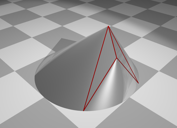
Figure 1: Visualization of the perturbed surface.

In the following, we derive an expansion formula of the resistance of the perturbed body in terms of the parameter $\varepsilon$. Note that the original cone corresponds to $\varepsilon=0$.

Since the resistance does not change under rotations and reflections, we can assume without loss of generality, that the line through the points $(x_{0},y_{0})$ and $(x_{1},y_{1})$ also contains the point $(1,0)$ and that $y_{0}\geq 0$.

The line $P_{0}P_{1}$ intersects the horizontal plane $\{z=0\}$ at the point

$$\begin{pmatrix}x_{2}\\ y_{2}\end{pmatrix}=\frac{m}{m-1}\begin{pmatrix}x_{0}\\ y_{0}\\ \end{pmatrix}+\frac{1}{1-m}\begin{pmatrix}x_{1}\\ y_{1}\\ \end{pmatrix}.$$

The perturbed body can be described by the four parameters $x_{0}$, $y_{0}$, $M_{1}\in(0,1)$ and $\varepsilon>0$, since the point $P_{1}$ is given by

$$x_{1}=1-M_{1}+x_{0}M_{1}\quad\text{and}\quad y_{1}=M_{1}y_{0}.$$

Plugging this into the above equation, we find

$$\begin{pmatrix}x_{2}\\ y_{2}\\ \end{pmatrix}=\frac{1}{1-\varepsilon^{2}}\begin{pmatrix}1-\varepsilon^{2}x_{0}\\ -\varepsilon^{2}y_{0}\\ \end{pmatrix}.$$

Next, we write the point $P_{2}$ in polar coordinates, i.e., $(x_{2},y_{2})=r_{2}\,(\cos\theta_{2},\sin\theta_{2})$ with

$$r_{2}^{2}=\frac{1-2\varepsilon^{2}x_{0}+\varepsilon^{4}(x_{0}^{2}+y_{0}^{2})}{(1-\varepsilon^{2})^{2}}\quad\mbox{and}\quad\theta_{2}=-\arctan\frac{\varepsilon^{2}y_{0}}{1-\varepsilon^{2}x_{0}},$$

where we used $y_{2}\leq 0$. We compute some parameters to describe the structure of the perturbed body. The circle $\partial\Omega$ contains two important points $(\cos\varphi_{\pm},\sin\varphi_{\pm})$, where $\pm\varphi_{\pm}>0$ and $\varphi_{\pm}\to 0$ as $\varepsilon\to+0$. These are the tangent points of the tangent lines to the unit disc passing through $(x_{2},y_{2})$. The lateral boundary of the body consists of the following parts:

1. A big conic surface with apex $(x_{0},y_{0},-1)$ and boundary arc $(\cos\varphi,\sin\varphi,0)$ for $\varphi\in[\varphi_{+},\varphi_{-}+2\pi]$. Let us compute the total resistance of this surface. We parametrize this part of the boundary via

   $$\begin{pmatrix}x\\ y\\ z\end{pmatrix}=\begin{pmatrix}(1-\lambda)x_{0}+\lambda\cos\varphi\\ (1-\lambda)y_{0}+\lambda\sin\varphi\\ -(1-\lambda)\end{pmatrix},\qquad\lambda\in[0,1],\varphi\in[\varphi_{+},\varphi_{-}+2\pi].$$

   Note that a normal vector of this surface is given by

   $$n=\begin{pmatrix}\cos\varphi&\sin\varphi&x_{0}\cos\varphi+y_{0}\sin\varphi-1\end{pmatrix}^{\top},$$

   hence we have $|\nabla u(x,y)|=1/(1-x_{0}\cos\varphi-y_{0}\sin\varphi)$, where $(x,y)$ is linked with $(\lambda,\varphi)$ via the above parametrization. For the area of the surface element, we get

   $$\mathrm{d}x\wedge\mathrm{d}y=\lambda\,(1-x_{0}\cos\varphi-y_{0}\sin\varphi)\,\mathrm{d}\lambda\wedge\mathrm{d}\varphi.$$

   Hence, the total resistance is given by

   $$R_{0} =\int_{0}^{1}\lambda\,\mathrm{d}\lambda\left(\int_{0}^{2\pi}-\int_{\varphi_{-}}^{\varphi_{+}}\right)\frac{1-x_{0}\cos\varphi-y_{0}\sin\varphi}{(1-x_{0}\cos\varphi-y_{0}\sin\varphi)^{-2}+\delta}\,\mathrm{d}\varphi$$

   $$=\frac{1}{2}\left(\int_{0}^{2\pi}-\int_{\varphi_{-}}^{\varphi_{+}}\right)\frac{(1-x_{0}\cos\varphi-y_{0}\sin\varphi)^{3}}{1+\delta(1-x_{0}\cos\varphi-y_{0}\sin\varphi)^{2}}\,\mathrm{d}\varphi.$$

2. A small conic surface consisting of the apex $(x_{1},y_{1},-m)$ and the boundary arc $(\cos\varphi,\sin\varphi,0)$ for $\varphi\in[\varphi_{-},\varphi_{+}]$. Similarly, we arrive at

   $$R_{1}=\frac{1}{2}\int_{\varphi_{-}}^{\varphi_{+}}\frac{(1-x_{1}\cos\varphi-y_{1}\sin\varphi)^{3}}{m^{2}+\delta(1-x_{1}\cos\varphi-y_{1}\sin\varphi)^{2}}\,\mathrm{d}\varphi.$$

3. Two triangles with vertices $(x_{0},y_{0},-1)$, $(x_{1},y_{1},-m)$ and $(\cos\varphi_{\pm},\sin\varphi_{\pm},0)$. On these triangles we have $\nabla u_{\pm}=1/(1-x_{0}\cos\varphi_{\pm}-y_{0}\sin\varphi_{\pm})$. The areas of their projections onto the plane $\{z=0\}$ are

   $$S_{\pm}=\pm\frac{1}{2}\det\begin{bmatrix}\cos\varphi_{\pm}-x_{0}&\cos\varphi_{\pm}-x_{1}\\ \sin\varphi_{\pm}-y_{0}&\sin\varphi_{\pm}-y_{1}\end{bmatrix}.$$

Hence, the total resistance of the perturbed body is given by the expression

$$\mathfrak{R}(\varepsilon)=R_{0}+R_{1}+\frac{S_{+}}{\lvert\nabla u_{+}\rvert^{2}+\delta}+\frac{S_{-}}{\lvert\nabla u_{-}\rvert^{2}+\delta}.$$

In what follows, we will derive an asymptotic expansion of $R$ as $\varepsilon\searrow 0$. Note that the resistance of the unperturbed body is given by

$$\mathfrak{R}(0)=R_{0}(0)=\frac{1}{2}\int_{0}^{2\pi}\frac{(1-x_{0}\cos\varphi-y_{0}\sin\varphi)^{3}}{1+\delta(1-x_{0}\cos\varphi-y_{0}\sin\varphi)^{2}}\,\mathrm{d}\varphi.$$

It is easy to see that

$$\varphi_{\pm}=\theta_{2}\pm\arccos\frac{1}{r_{2}}=-\arctan\frac{\varepsilon^{2}y_{0}}{1-\varepsilon^{2}x_{0}}\pm\arccos\frac{1-\varepsilon^{2}}{\sqrt{1-2\varepsilon^{2}x_{0}+\varepsilon^{4}(x_{0}^{2}+y_{0}^{2})}}.$$

This right-hand side cannot be used to obtain an expansion of $\varphi_{\pm}$, since the argument of $\arccos$ goes to 1 as $\varepsilon\searrow 0$. Nonetheless, by using the addition theorems for cosine and sine, a straightforward computation gives

$$\cos\varphi_{\pm}=\frac{(1-x_{0}\varepsilon^{2})(1-\varepsilon^{2})\pm y_{0}\varepsilon^{3}\sqrt{2(1-x_{0})-(1-x_{0}^{2}-y_{0}^{2})\varepsilon^{2}}}{1-2\varepsilon^{2}x_{0}+\varepsilon^{4}(x_{0}^{2}+y_{0}^{2})},$$

$$\sin\varphi_{\pm}=\frac{\pm(1-x_{0}\varepsilon^{2})\varepsilon\sqrt{2(1-x_{0})-(1-x_{0}^{2}-y_{0}^{2})\varepsilon^{2}}-y_{0}(1-\varepsilon^{2})\varepsilon^{2}}{1-2\varepsilon^{2}x_{0}+\varepsilon^{4}(x_{0}^{2}+y_{0}^{2})}.$$

Using the last formula, we see that $\pm\varphi_{\pm}=\varepsilon\,\sqrt{2\,(1-x_{0})}+O(\varepsilon^{2})$ as $\varepsilon\to+0$. Note that $\varphi_{\pm}$ were initially defined for $\varepsilon\geq 0$. However, they are analytic functions of $\varepsilon\geq 0$ as $\arcsin$ is analytic. Hence, we are able to extend their domains for $\varepsilon<0$ by analyticity. Both $\varphi_{+}$ and $\varphi_{-}$ become analytic functions of $\varepsilon$ around $0$. Moreover, $\varphi_{+}(-\varepsilon)=\varphi_{-}(\varepsilon)$

First, let us compute expansions for the integrals appearing in $R_{0}$ and $R_{1}$. Using the Leibniz integral rule, we arrive at

$$\frac{1}{2}\int_{\varphi_{-}(\varepsilon)}^{\varphi_{+}(\varepsilon)}\frac{(1-x_{0}\cos\varphi-y_{0}\sin\varphi)^{3}}{1+\delta(1-x_{0}\cos\varphi-y_{0}\sin\varphi)^{2}}\,\mathrm{d}\varphi=\frac{\sqrt{2}(1-x_{0})^{7/2}}{1+\delta(1-x_{0})^{2}}\varepsilon+O(\varepsilon^{2}).$$ (6)

Similarly, using $m=M_{1}+\varepsilon^{2}(1-M_{1})$, the following expansion can be computed by converting the fraction under the integral into a Taylor series

$$\frac{1}{2}\int_{\varphi_{-}(\varepsilon)}^{\varphi_{+}(\varepsilon)}\frac{(1-x_{1}\cos\varphi-y_{1}\sin\varphi)^{3}}{m^{2}+\delta(1-x_{1}\cos\varphi-y_{1}\sin\varphi)^{2}}\,\mathrm{d}\varphi$$ (7)

$$\qquad=\frac{1}{2}\int_{\varphi_{-}(\varepsilon)}^{\varphi_{+}(\varepsilon)}\frac{(1-x_{1}\cos\varphi-y_{1}\sin\varphi)^{3}}{M_{1}^{2}+\delta(1-x_{1}\cos\varphi-y_{1}\sin\varphi)^{2}}\,\mathrm{d}\varphi+O(\varepsilon^{2})$$

$$\qquad=\frac{\sqrt{2}(1-x_{0})^{1/2}(1-x_{1})^{3}}{M_{1}^{2}+\delta(1-x_{1})^{2}}+O(\varepsilon^{2})=\frac{M_{1}\sqrt{2}(1-x_{0})^{7/2}}{1+\delta(1-x_{0})^{2}}\varepsilon+O(\varepsilon^{2}).$$

In the last step, we used $1-x_{1}=M_{1}(1-x_{0})$. Moreover, both integrals are odd analytic function of $\varepsilon$, since $\varphi_{+}(-\varepsilon)=\varphi_{-}(\varepsilon)$ and the integrand in (7) is an even function w.r.t. $\varepsilon$. Hence, the remainder terms in (6) and (7) are actually $O(\varepsilon^{3})$.

Second, we consider the triangles. Using again $\varphi_{+}(-\varepsilon)=\varphi_{-}(\varepsilon)$, we have $\nabla u_{+}(-\varepsilon)=\nabla u_{-}(\varepsilon)$ and $S_{+}(-\varepsilon)=-S_{-}(\varepsilon)$. Hence, $\frac{S_{+}}{\lvert\nabla u_{+}\rvert^{2}+\delta}+\frac{S_{-}}{\lvert\nabla u_{-}\rvert^{2}+\delta}$ is an odd function of $\varepsilon$. To expand $\nabla u_{\pm}=1/(1-x_{0}\cos\varphi_{\pm}-y_{0}\sin\varphi_{\pm})$, we use

$$1-x_{0}\cos\varphi_{\pm}-y_{0}\sin\varphi_{\pm}$$

$$\qquad=\frac{1-x_{0}\mp y_{0}\varepsilon\sqrt{2(1-x_{0})-(1-x_{0}^{2}-y_{0}^{2})\varepsilon^{2}}+(x_{0}^{2}+y_{0}^{2}-x_{0})\varepsilon^{2}}{1-2\varepsilon^{2}x_{0}+\varepsilon^{4}(x_{0}^{2}+y_{0}^{2})}$$

$$\qquad=1-x_{0}\mp y_{0}\sqrt{2(1-x_{0})}+O(\varepsilon^{2})$$ (8)

and

$$S_{\pm}=\frac{1}{2}(1-M_{1})(1-x_{0})\sqrt{2(1-x_{0})}\,\varepsilon+O(\varepsilon^{2}).$$ (9)

Thus,

$$\frac{S_{\pm}}{\lvert\nabla u_{\pm}\rvert^{2}+\delta}=\frac{(1-M_{1})(1-x_{0})^{7/2}}{\sqrt{2}(\delta(1-x_{0})^{2}+1)}\varepsilon+O(\varepsilon^{2}),$$

and

$$\frac{S_{+}}{\lvert\nabla u_{+}\rvert^{2}+\delta}+\frac{S_{-}}{\lvert\nabla u_{-}\rvert^{2}+\delta}=\frac{\sqrt{2}(1-M_{1})(1-x_{0})^{7/2}}{\delta(1-x_{0})^{2}+1}\varepsilon+O(\varepsilon^{3}).$$ (10)

By combining (6), (7) and (10), we have

$$\mathfrak{R}(\varepsilon)-\mathfrak{R}(0)=O(\varepsilon^{3}).$$

Hence, a first-order Taylor expansion of $\mathfrak{R}$ does not yield enough information and we have to use a higher order Taylor expansion. As we mentioned, $\mathfrak{R}(\varepsilon)$ is odd analytic in $\varepsilon$. Thus, also the second-order term vanishes and the third-order term can be computed in a similar way by expanding (6)–(10) up to the $\varepsilon^{3}$ terms. We arrive at

$$\frac{\mathfrak{R}(\varepsilon)-\mathfrak{R}(0)}{(1-x_{0})^{5/2}}$$

$$\qquad=\frac{4(1-M_{1})\sqrt{2}}{3(1+\delta(1-x_{0})^{2})^{3}}\left[3y_{0}^{2}-(1-x_{0})^{2}-\delta(1-x_{0})^{2}((1-x_{0})^{2}+y_{0}^{2})\right]\varepsilon^{3}$$

$$\qquad\qquad+O(\varepsilon^{5}).$$

Thereby, since $\varepsilon>0$, we obtain that the sign of the variation of the resistance coincides with the sign of the expression

$$3y_{0}^{2}-(1-x_{0})^{2}-\delta(1-x_{0})^{2}((1-x_{0})^{2}+y_{0}^{2}),$$

in case that this expression is not zero. It is interesting to note that the parameter $M_{1}$ does not appear. Recall that we were assuming $x_{2}=1$ and $y_{2}=0$. For an arbitrary case, we must rotate the body in such a way that the point $(x_{2},y_{2})$ will coincide with $(1,0)$.

Theorem 6.

Let $u\in\hat{C}$ and $\delta\geq 0$. Suppose that $u$ contains a conical part made up by the convex hull of a vertex $(x_{0},y_{0},-z_{0})$ ($z_{0}>0$ and $(x_{0},y_{0})=(r_{0}\cos\varphi_{0},r_{0}\sin\varphi_{0})$ with $0\leq r_{0}<1$) and an arc $(\cos\varphi,\sin\varphi,0)\in\partial\Omega$ for $\varphi\in[\alpha,\beta]$ with $\alpha<\beta$. If there exists $\varphi\in[\alpha,\beta]$ such that

$$\frac{3r_{0}^{2}\sin^{2}(\varphi-\varphi_{0})-[1-r_{0}\cos(\varphi-\varphi_{0})]^{2}}{[1-r_{0}\cos(\varphi-\varphi_{0})]^{2}[1+r_{0}^{2}-2r_{0}\cos(\varphi-\varphi_{0})]}<\delta z_{0}^{-2}.$$ (11)

Then $u$ is not optimal for $J_{M}$ with $M=\delta^{-1/2}$ for $\delta>0$ and $M=\infty$ for $\delta=0$

Proof.

The left-hand side of (11) is continuous w.r.t. $\varphi$. Thus, w.l.o.g., we suppose $\varphi\in(\alpha,\beta)$. In order to apply the above arguments, we rotate and rescale the function $u$ via $\tilde{u}(x,y)=u(x\cos\varphi+y\sin\varphi,-x\sin\varphi+y\cos\varphi)/z_{0}$. Then, $J_{M}(u)=z_{0}^{-2}J_{z_{0}M}(\tilde{u})$. The function $\tilde{u}$ contains a conical part made up by the apex $(X_{0},Y_{0},-1)$ with

$$X_{0} =\phantom{-{}}x_{0}\cos\varphi+y_{0}\sin\varphi=r_{0}\cos(\varphi-\varphi_{0});$$

$$Y_{0} =-x_{0}\sin\varphi+y_{0}\cos\varphi=r_{0}\sin(\varphi-\varphi_{0});$$

and an arc on the unit circle $\partial\Omega\times\{0\}$ containing point $(1,0,0)$ in its interior. Hence, applying the variation described in the beginning of the present section to $\tilde{u}$, we obtain that the change of the cost functional $J_{z_{0}M}(\tilde{u})$ has the same sign as

$$3Y_{0}^{2}-(1-X_{0})^{2}-\tilde{\delta}(1-X_{0})^{2}((1-X_{0})^{2}+Y_{0}^{2})$$

where $\tilde{\delta}=(Mz_{0})^{-2}=\delta\,z_{0}^{-2}$. Due to (11), the variation has a negative sign. Hence, $\tilde{u}$ is not optimal for $J_{z_{0}\,M}$ and, consequently, $u$ is not optimal for $J_{M}$. ∎

We denote the left-hand side of inequality (11) by $Z_{0}(r_{0},\Delta\varphi)$, where $\Delta\varphi=\varphi-\varphi_{0}$. In case $\delta=0$, non-optimality occurs if $Z_{0}(r_{0},\Delta\varphi)<0$. In case $\delta>0$, the condition (11) is equivalent to

$$Mz_{0}<\begin{cases}\infty&\text{if }Z_{0}(r_{0},\Delta\varphi)\leq 0\\ Z_{0}(r_{0},\Delta\varphi)^{-1/2}&\text{if }Z_{0}(r_{0},\Delta\varphi)>0.\end{cases}$$

In Fig. 2, we plotted some level sets of $Z_{0}(r_{0},\Delta\varphi)^{-1/2}$ and the level set $Z_{0}(r_{0},\Delta\varphi)=0$ (labeled with $\infty$) in the polar coordinates $(r_{0},\Delta\varphi)$.

Figure 2: This shows some level sets of the function $Z_{0}(r_{0},\Delta\varphi)^{-1/2}$, see (11), in the polar coordinate system $(r_{0},\Delta\varphi)$.

6 applies to the rescaled version of Newton’s problem. For later reference, we also give a formulation which can be directly applied to the original problem (1).

Corollary 7.

Let $M\geq 0$ and $u\in C_{M}$ be given. Suppose that $u$ contains a conical part made up by the convex hull of a vertex $(x_{0},y_{0},-z_{0})$ ($z_{0}>0$ and $(x_{0},y_{0})=(r_{0}\cos\varphi_{0},r_{0}\sin\varphi_{0})$ with $0<r_{0}<1$) and a boundary arc $(\cos\varphi,\sin\varphi,0)\in\partial\Omega$ for $\varphi\in[\alpha,\beta]$ with $\alpha<\beta$. If there exists $\varphi\in[\alpha,\beta]$ such that

$$\frac{3r_{0}^{2}\sin^{2}(\varphi-\varphi_{0})-[1-r_{0}\cos(\varphi-\varphi_{0})]^{2}}{[1-r_{0}\cos(\varphi-\varphi_{0})]^{2}[1+r_{0}^{2}-2r_{0}\cos(\varphi-\varphi_{0})]}<z_{0}^{-2}.$$ (12)

Then $u$ is not optimal for $J$.

6 Non-optimality in the Class of all Convex Function of Suggested Solutions in the Literature

In this section, we apply Corollary 7 to some conjectured solutions. In particular, we address the contributions LachandRobertPeletier2001 (10, 16, 12).

6.1 Conjectured solutions by LachandRobertPeletier2001 (10) (10)

We proceed in chronological order and start with the bodies given in LachandRobertPeletier2001 (10). Therein, the authors studied Newton’s problem in a restricted class of functions and obtained bodies which are the convex hull of $\Omega\times\{0\}\cup N_{0}\times\{-M\}$, where $N_{0}\subset\mathbb{R}^{2}$ is a regular polygon centered at $0$. We note that the (global) non-optimality of these bodies was already observed in LachandNumeric (8, 16) via the comparison with the numerical solutions. We will check that the (local) non-optimality also follows from Corollary 7. Let us assume that $N_{0}$ is a regular polygon with $k\geq 2$ vertices and we rotate $N_{0}$ such that one vertex is given by $(x_{0},0)$ for some $x_{0}\in(0,1)$. Then, it is clear that the body contains a conical part with parameters

$$(x_{0},y_{0},z_{0}) =(x_{0},0,-M)=(r_{0}\cos\varphi_{0},r_{0}\sin\varphi_{0},-M) r_{0} =x_{0},$$

$$\varphi_{0} =0, \beta =-\alpha=\pi/k.$$

The body with $M=1.0$ is shown in Fig. 3 (top left).

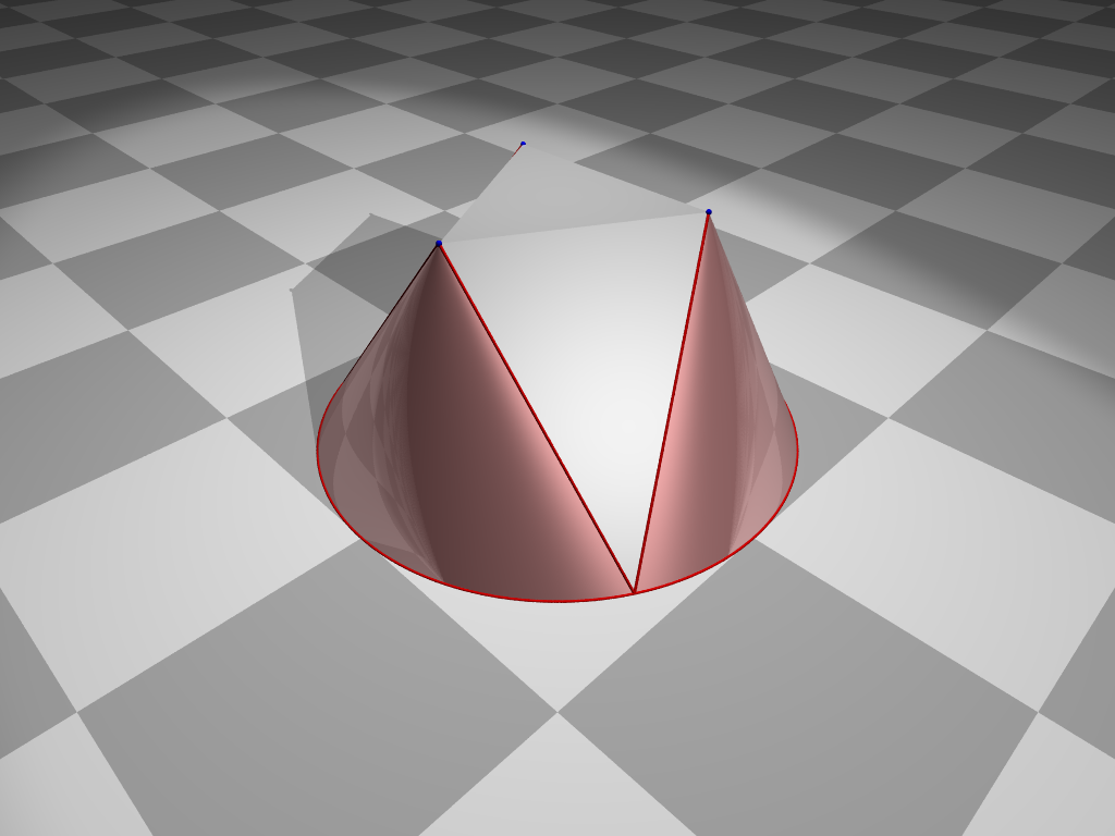
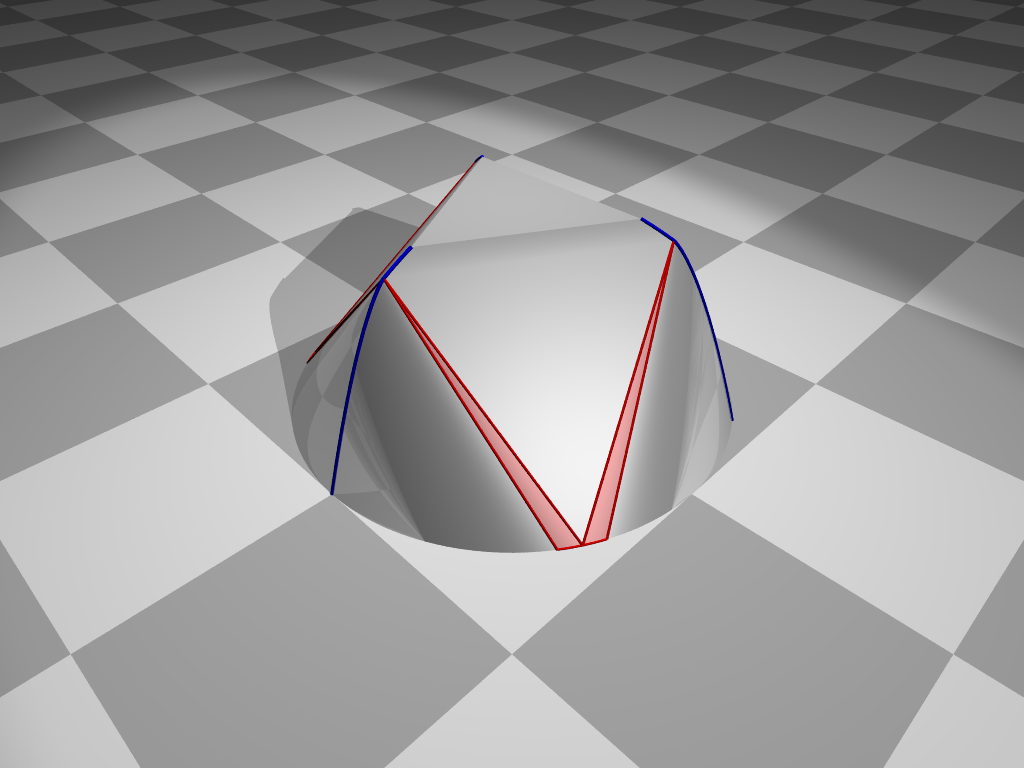
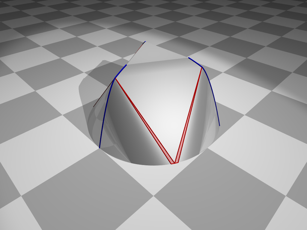
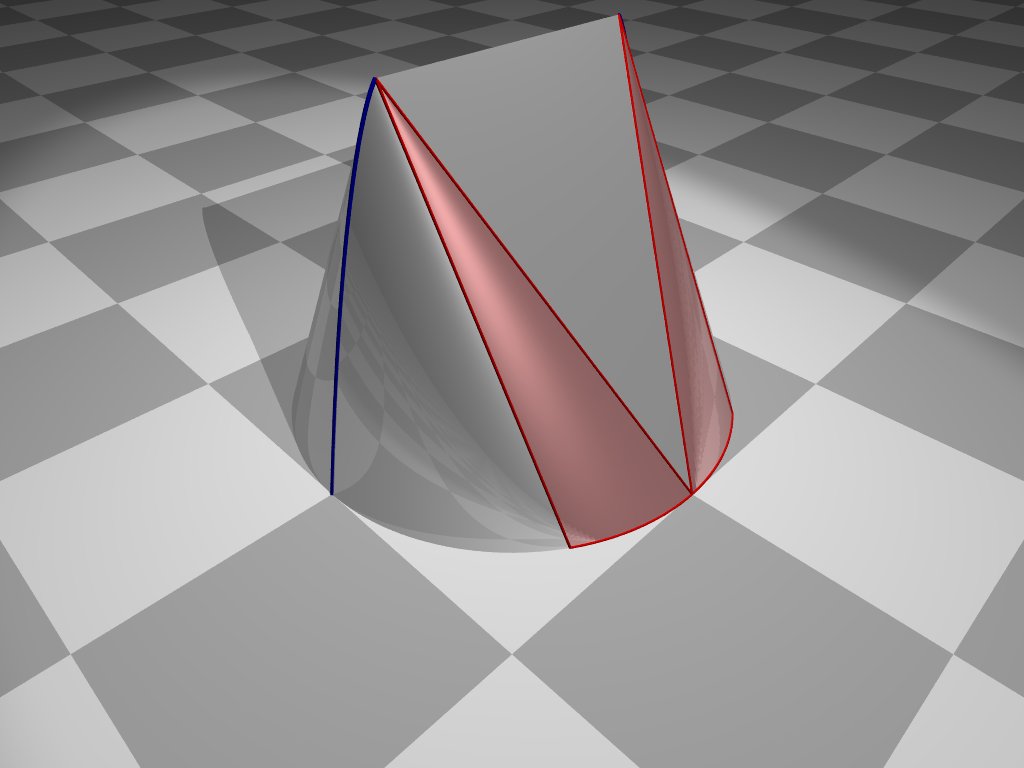
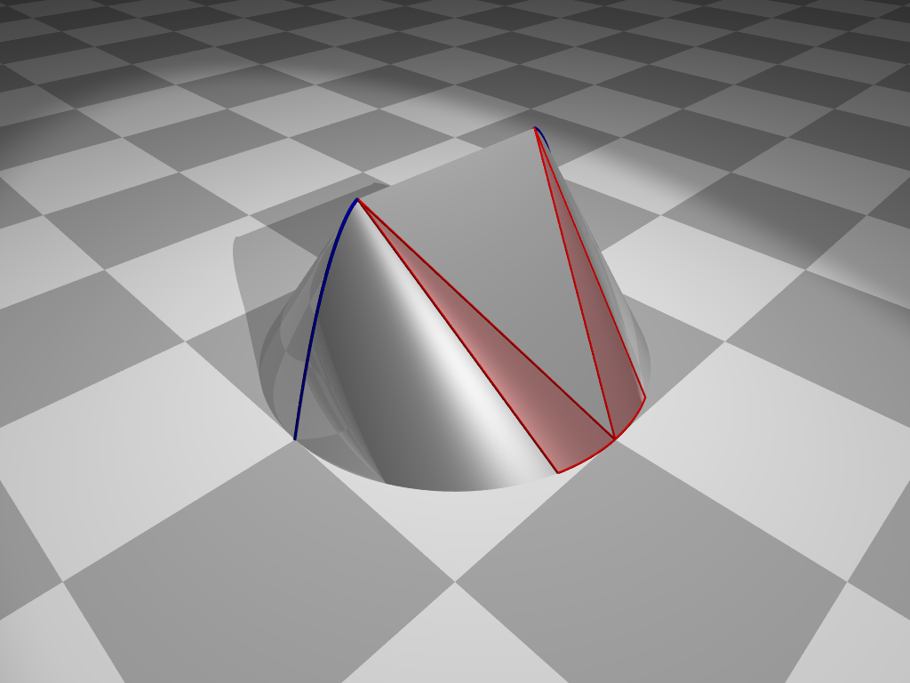
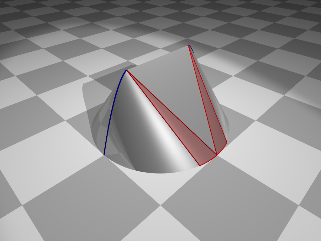
Figure 3: Illustration of conjectured solutions (shown upside down) containing non-optimal conical parts (highlighted red): LachandRobertPeletier2001 (10) with $M=1.0$ (top left), Wachsmuth (16) with $(M,k)=(0.9,3)$ (top right) and with $(M,k)=(1.0,3)$ (middle left), LokutsievskiyZelikin2 (12) with $M=1.5$ (middle right), $M=5.0$ (bottom left), $M=\infty$ (bottom right). The bodies in the bottom row are rescaled to height $1.0$, cf. (2). All the bodies are constructed as the convex hull of the blue points and the base $\Omega\times\{0\}$.

Now, it is easy to check that the left-hand side of inequality (12) is negative for $\varphi=0\in(\alpha,\beta)$ and, therefore, (12) holds true.

Hence, the bodies suggested by LachandRobertPeletier2001 (10) (10) cannot be optimal for any value of $M>0$ and $k\geq 2$.

6.2 Conjectured solutions by Wachsmuth (16) (16)

Next, we investigate the structural conjecture from (Wachsmuth, 16, Section 3) where the author has supposed that optimal bodies for a height $M\in(0,\bar{M})$, with $\bar{M}\in(1.4,1.5)$, have the following structure. There exists $k\in\mathbb{N}$, $k\geq 3$, and a convex function $g\colon[0,1]\to[-M,0]$, $g(0)=-M$, $g(1)=0$, such that the optimal body is the convex hull of the set

$$\partial\Omega\times\{0\}\cup\{(r\,\cos(2\,i\,\varphi),r\,\sin(2\,i\,\varphi),g(r)),\;i=0,\ldots,k-1,\;r\in[0,1]\},$$

where $\varphi=\pi/k$. Examples with $M=1.0$ and $M=0.9$ are depicted in Fig. 3 (top right and middle left). The extremal lines

$$\{(r\,\cos(2\,i\,\varphi),r\,\sin(2\,i\,\varphi),g(r)),\;i=0,\ldots,k-1,\;r\in[0,1]\}$$

are highlighted in blue. Under some natural assumptions on $g$, the problem becomes a one-dimensional problem of calculus of variations and can be solved for $g$ by the corresponding Euler-Lagrange equations. The obtained class of solutions contains a conical part (denoted by Region II therein), see (Wachsmuth, 16, Figure 6) and Fig. 3 (middle left). However, for the results presented in (Wachsmuth, 16, Table 3) (reproduced and extended in Table 1), only the solution corresponding to $M=1.0$ (the height parameter is denoted by $L$ in Wachsmuth (16)) and symmetry parameter $k=3$ (denoted by $m$ in Wachsmuth (16)) contains this conical part and for all other presented solutions, this conical part vanishes. Moreover, it can be checked that Corollary 7 applies to this solution with $M=1.0$ and $k=3$. Hence, the structural conjecture of Wachsmuth (16) cannot be true for this height $M=1.0$.

The (non-optimal) body from (Wachsmuth, 16, Section 3) with $(M,k)=(1.0,3)$ is displayed in Fig. 3 (middle left). Note that the conical parts are rather small. We believe that the non-optimality of this body is (informally speaking) only due to these small conical parts. Therefore, we expect that the objective value can be improved only by a small amount and this seems to be hard to achieve via numerical methods. We also show the body corresponding to $(M,k)=(0.9,3)$ (top right) which has a larger conical part.

In Table 1, we present an updated and completed version of (Wachsmuth, 16, Table 3).

$M$ \ $k$	3	4	5	6	7	8
$1.5$	$0.6999489$	$0.7123013$	$0.7218282$	$0.7285828$	$0.7334158$	$0.7369567$
$1.4$	$0.7677364$	$0.7792767$	$0.7887148$	$0.7955246$	$0.8004380$	$0.8040548$
$1.3$	$0.8441426$	$0.8544163$	$0.8635882$	$0.8703656$	$0.8753090$	$0.8789708$
$1.2$	$0.9303614$	$0.9387924$	$0.9474690$	$0.9540986$	$0.9590059$	$0.9626708$
$1.1$	$1.0277294$	$1.0335975$	$1.0414890$	$1.0478237$	$1.0526095$	$1.0562233$
$1.0$	$1.1377294$ CN	$1.1401510$	$1.1468980$	$1.1527533$	$1.1573095$	$1.1608036$
$0.9$	$1.2619895$ CN	$1.2599052$	$1.2650665$	$1.2702151$	$1.2744081$	$1.2776964$
$0.8$	$1.4022724$ CN	$1.3944389$	$1.3974884$	$1.4016551$	$1.4053219$	$1.4082995$
$0.7$	$1.5604532$ CN	$1.5454605$	$1.5457807$	$1.5486392$	$1.5515845$	$1.5541263$
$0.6$	$1.7392117$ CN	$1.7147979$	$1.7116824$	$1.7128535$	$1.7148496$	$1.7168060$
$0.5$	$1.9438498$ CN	$1.9043842$	$1.8970564$	$1.8961062$	$1.8968909$	$1.8980899$
$0.4$	$2.1775037$ CN	$2.1176695$ C	$2.1038722$	$2.1003292$	$2.0996063$	$2.0998537$
$0.3$	$2.4390875$ CN	$2.3611648$ CN	$2.3354683$ C	$2.3276201$ C	$2.3250270$	$2.3241056$
$0.2$	$2.7171218$ CN	$2.6385156$ CN	$2.5993030$ C	$2.5828003$ C	$2.5760193$ C	$2.5731257$ C
$0.1$	$2.9786691$ CN	$2.9338815$ CN	$2.8990387$ CN	$2.8754404$ CN	$2.8612811$ C	$2.8533036$ C

Table 1: Conjectured optimal values using the conjecture from (Wachsmuth, 16, Section 3). A “C” indicates that this solution contains a conical part. For the solutions marked by “N”, Corollary 7 applies and, therefore, those solutions cannot be optimal in the class of all convex bodies $C_{M}$. The minimal (conjectured) solutions for each $M$ are underlined.

In this table, we underlined the best solution in each row, i.e. for each height parameter $M$. Note that for $M=1.5$ a better solution was obtained numerically in (Wachsmuth, 16, Section 2) whereas for $M\leq 0.3$ a structured solution with $k=9$ produces better values than the solutions given in the table. Hence, we do not underline solutions in the lines corresponding to $M=1.5$ and $M\leq 0.3$.

For each solution presented in Table 1, we checked whether this solution contains a conical part (indicated by “C”) and whether Corollary 7 applies to this conical part and provides the non-optimality (indicated by “N”). For each fixed $k$ it seems that conical parts appear for small values of $M$ (depending on $k$) and that, eventually, this conical part becomes non-optimal. However, for $k\geq 4$ the non-optimality appears only for “very small” values of $M$ and for these values, $k+1$ provides a better solution. Hence, for $M\leq 0.9$ (and, therefore, $k\geq 4$) we cannot apply Corollary 7 and we cannot disprove the conjecture of (Wachsmuth, 16, Section 3). For $M$ between $1.0$ and $1.4$ the situation is different. Here, the best results (according to the structural conjecture of (Wachsmuth, 16, Section 3)) are obtained by $k=3$ and these contain non-optimal conical parts for heights $M$ that are smaller than approximately $1.0$. In particular, we can apply Corollary 7 for the height $M=1.0$ and therefore, the conjecture of (Wachsmuth, 16, Section 3) is disproved for this value. For $M$ bigger than $1.1$, the solutions with $k=3$ do not contain conical parts and therefore, we cannot disprove the conjecture for $M$ between $1.1$ and $1.4$.

In Table 2, we list some more values for $M\in[0.9,1.1]$ and $k\in\{3,4\}$.

$M$ \ $k$	3	4
$1.10$	$1.0277294$	$1.0335975$
$1.09$	$1.0381352$ C	$1.0437014$
$1.08$	$1.0486688$ CN	$1.0539240$
$1.07$	$1.0593317$ CN	$1.0642667$
$1.06$	$1.0701256$ CN	$1.0747311$
$1.05$	$1.0810520$ CN	$1.0853184$
$1.04$	$1.0921125$ CN	$1.0960303$
$1.03$	$1.1033089$ CN	$1.1068681$
$1.02$	$1.1146427$ CN	$1.1178333$
$1.01$	$1.1261157$ CN	$1.1289274$
$1.00$	$1.1377294$ CN	$1.1401510$

$M$ \ $k$	3	4
$1.00$	$1.1377294$ CN	$1.1401510$
$0.99$	$1.1494856$ CN	$1.1515072$
$0.98$	$1.1613861$ CN	$1.1629969$
$0.97$	$1.1734324$ CN	$1.1746215$
$0.96$	$1.1856264$ CN	$1.1863837$
$0.95$	$1.1979697$ CN	$1.1982830$
$0.94$	$1.2104642$ CN	$1.2103218$
$0.93$	$1.2231117$ CN	$1.2225019$
$0.92$	$1.2359138$ CN	$1.2348243$
$0.91$	$1.2488725$ CN	$1.2472919$
$0.90$	$1.2619895$ CN	$1.2599052$

Table 2: Similar as Table 1, but for different values of $M$ and $k$.

This table suggests the following observations:

• For $M\geq 1.09$, the bodies conjectured in (Wachsmuth, 16, Section 3) might be optimal since these bodies do not contain conical parts or their conical parts do not satisfy Corollary 7.

• For $M\in[0.95,1.08]$, the conjectured optimal bodies contain a non-optimal conical part and, therefore, the structural conjecture of (Wachsmuth, 16, Section 3) is disproved for these values of $M$.

• For $M\in[0.90,0.94]$, our non-optimality result does not apply to the conjectured bodies with $k=4$ and these bodies possess better values than those with $k=3$. However, the bodies with symmetry parameter $k=3$ are not locally optimal in $C_{M}$ by Corollary 7. It is also clear that our variation from Section 5 can be modified to produce bodies with a threefold symmetry which possess smaller objective values than those indicated in Table 2 for $k=3$. In particular, these improved values could be smaller than the corresponding values with $k=4$ from Table 2 and this would disprove the structural conjecture of Wachsmuth (16) for some values of $M$ around $0.94$. This is subject to future research.

To summarize, Corollary 7 disproves the conjectured bodies from (Wachsmuth, 16, Section 3) at least for $M\in[0.95,1.08]$, see Table 2. It does not apply for $M\leq 0.94$ and $M\in[1.09,1.4]$, and for these values, the conjecture might be true.

6.3 Conjectured solutions by LokutsievskiyZelikin2 (12) (12)

In LokutsievskiyZelikin2 (12), the authors study the class $E_{M}$ of convex bodies of height $M$ which can be written as the convex hull of the union of the base $\Omega\times\{0\}$ and of a convex curve $z=v^{*}(x_{1})$ in the plane $\{x_{2}=0\}$ (we keep notations of LokutsievskiyZelikin2 (12), and $v^{*}$ denotes the Legendre-Young-Fenchel transform of a convex function $v$). We note that this approach is similar to Section 6.2 with $k=2$. The authors proved local optimality of such bodies in the corresponding class (see (LokutsievskiyZelikin2, 12, Theorem 9.1)).

In this paper, there is a table with numerically found parameters of the locally optimal curve $v^{*}$ for some different values of the height $M$ (see (LokutsievskiyZelikin2, 12, Table 1)). The solution $v^{*}$ has a horizontal line segment in the front of the body, since $v$ has a corner at $0$. It can be checked that all the bodies from the table contain a conical part. Exemplarily, we have shown the bodies corresponding to $M=1.5$ in Fig. 3 (middle right) and to $M=5.0$ (rescaled to height $1.0$, bottom left). The conical part is given by the vertex $(x_{0},y_{0},z_{0})=(v^{\prime}(+0),0,-M)$ and the arc with angles $[\alpha,\beta]=[\pi/2-\varepsilon,\pi/2]$ for some $\varepsilon>0$. Now, it is easily checked that inequality (12) from Corollary 7 is fulfilled for $r_{0}=v^{\prime}(+0)$, $\varphi_{0}=0$, $\varphi=\beta=\pi/2$ and $z_{0}=M$. Therefore, this conical part is always non-optimal in the class $C_{M}$ of all convex bodies. Hence, it seems that the optimal bodies in the class $E_{M}$ are never optimal in $C_{M}$.

A similar approach can be used for the limiting problem of minimizing $J_{\infty}$ in the class $E_{1}$. Using the same strategy, one obtains the values (with the notation of LokutsievskiyZelikin2 (12))

$$p_{0} \approx 3.167203701258, r(p_{0}) \approx 0.3451623687826,$$

$$v^{\prime}(+0) \approx 0.5300674211893, J_{\infty}(u) \approx 2.140225047120.$$

The corresponding body is shown in Fig. 3 (bottom right). Again, this body has a conical part (with $\varepsilon\approx 0.296085$), which is non-optimal by Corollary 7.

Thus, the minimizers of $J_{\infty}$ in $\hat{C}$ do not belong to $E_{1}$. Hence, the family found in LokutsievskiyZelikin2 (12) cannot be asymptotically optimal for $J$ in $C_{M}$ by 3 despite the fact that it is locally optimal in $E_{M}$ by (LokutsievskiyZelikin2, 12, Theorem 9.1).

Acknowledgement

Gerd Wachsmuth acknowledges fruitful discussions with Luca Landwehrjohann back in 2017 which spawned the seeds for some of the ideas in the present paper.

The work of Lev Lokutsievskiy was performed at the Steklov International Mathematical Center and supported by the Ministry of Science and Higher Education of the Russian Federation (agreement no. 075-15-2019-1614). The work of Gerd Wachsmuth was partially supported by the DFG Grant Approximation of Non-Smooth Optimal Convex Shapes with Applications in Optimal Insulation and Minimal Resistance (Grant No. WA 3636/5-2) within the Priority Program SPP 1962 (Non-smooth and Complementarity-based Distributed Parameter Systems: Simulation and Hierarchical Optimization). The work of Mikhail Zelikin was supported by Russian Foundation for Basic Research under grant 20-01-00469.

References

• (1) Gilbert A. Bliss “The Calculus of Variations for Multiple Integrals” In The American Mathematical Monthly 49.2 Mathematical Association of America, 1942, pp. 77–89 DOI: 10.1080/00029890.1942.11991185
• (2) Friedemann Brock, Vincenzo Ferone and Bernhard Kawohl “A symmetry problem in the calculus of variations” In Calculus of Variations and Partial Differential Equations 4.6 Springer ScienceBusiness Media LLC, 1996, pp. 593–599 DOI: 10.1007/bf01261764
• (3) Giuseppe Buttazzo “A survey on the Newton problem of optimal profiles” In Variational Analysis and Aerospace Engineering Springer New York, 2009, pp. 33–48 DOI: 10.1007/978-0-387-95857-6_3
• (4) Giuseppe Buttazzo, Vincenzo Ferone and Bernhard Kawohl “Minimum Problems over Sets of Concave Functions and Related Questions” In Mathematische Nachrichten 173.1 WILEY-VCH Verlag, 1995, pp. 71–89 DOI: 10.1002/mana.19951730106
• (5) Paolo Guasoni “Problemi di ottimizzazione di forma su classi di insiemi convessi”, 1996 URL: http://cvgmt.sns.it/paper/1146/
• (6) Jacques Hadamard “Sur quelques questions de calcul des variations” In Bulletin de la Société Mathématique de France 33 Société mathématique de France, 1905, pp. 73–80 DOI: 10.24033/bsmf.741
• (7) Wallace D. Hayes and Ronald F. Probstein “Hypersonic Flow Theory” Academic Press, 1964
• (8) Thomas Lachand-Robert and Édouard Oudet “Minimizing within Convex Bodies Using a Convex Hull Method” In SIAM Journal on Optimization, 16.2, 2005, pp. 368–379 DOI: 10.1137/040608039
• (9) Thomas Lachand-Robert and M.. Peletier “An example of non-convex minimization and an application to Newton’s problem of the body of least resistance” In Annales de l’I.H.P. Analyse non linéaire 18.2 Elsevier, 2001, pp. 179–198 URL: http://www.numdam.org/item/AIHPC_2001__18_2_179_0
• (10) Thomas Lachand-Robert and Mark A. Peletier “Newton’s Problem of the Body of Minimal Resistance in the Class of Convex Developable Functions” In Mathematische Nachrichten 226.1 Wiley, 2001, pp. 153–176 DOI: 10.1002/1522-2616(200106)226:1<153::aid-mana153>3.0.co;2-2
• (11) Lev V. Lokutsievskiy and Mikhail I. Zelikin “Hessian Measures in the Aerodynamic Newton Problem” In Dyn Control Syst 24, 2018, pp. 475–495 DOI: 10.1007/s10883-018-9395-x
• (12) Lev V. Lokutsievskiy and Mikhail I. Zelikin “The analytical solution of Newton’s aerodynamic problem in the class of bodies with vertical plane of symmetry and developable side boundary” In ESAIM: COCV 26, 2020 DOI: 10.1051/cocv/2019064
• (13) Isaac Newton “Philosophiæ Naturalis Principia Mathematica”, 1687
• (14) Alexander Plakhov “A note on Newton’s problem of minimal resistance for convex bodies”, 2019 arXiv:1908.01042
• (15) Alexander Plakhov “Method of nose stretching in Newton’s problem of minimal resistance”, 2020 arXiv:2003.06682 [math.OC]
• (16) Gerd Wachsmuth “The numerical solution of Newton’s problem of least resistance” In Mathematical Programming 147.1, 2014, pp. 331–350 DOI: 10.1007/s10107-014-0756-2
• (17) Черный Г.Г. “Газовая динамика” Москва: НАУКА, 1988