[table]capposition=top
The birth of the strong components111 This paper is an extended version of several earlier works by the authors. Some parts of this paper appeared in the 10th European Conference on Combinatorics, Graph Theory and Applications (EUROCOMB 2019), in the 32nd International Conference on Formal Power Series and Algebraic Combinatorics (FPSAC 2020), and in the 31st International Conference on Probabilistic, Combinatorial and Asymptotic Methods for the Analysis of Algorithms (AofA 2020), see [dPD19, dPD20, RRW20]. Authors are presented in alphabetical order.
Abstract
It is known that random directed graphs undergo a phase transition around the point . Earlier, Łuczak and Seierstad have established that as when , the asymptotic probability that the strongly connected components of a random directed graph are only cycles and single vertices decreases from 1 to 0 as goes from to .
By using techniques from analytic combinatorics, we establish the exact limiting value of this probability as a function of and provide more statistical insights into the structure of a random digraph around, below and above its transition point. We obtain the limiting probability that a random digraph is acyclic and the probability that it has one strongly connected complex component with a given difference between the number of edges and vertices (called excess). Our result can be extended to the case of several complex components with given excesses as well in the whole range of sparse digraphs.
Our study is based on a general symbolic method which can deal with a great variety of possible digraph families, and a version of the saddle point method which can be systematically applied to the complex contour integrals appearing from the symbolic method. While the technically easiest model is the model of random multidigraphs, in which multiple edges are allowed, and where edge multiplicities are sampled independently according to a Poisson distribution with a fixed parameter , we also show how to systematically approach the family of simple digraphs, where multiple edges are forbidden, and where 2-cycles are either allowed or not.
Our theoretical predictions are supported by numerical simulations when the number of vertices is finite, and we provide tables of numerical values for the integrals of Airy functions that appear in this study.
1 Introduction
Random graphs and directed graphs (digraphs) are omnipresent in many modern research areas such as computer science, biology, the study of social and technological networks, analysis of algorithms, and theoretical physics. Depending on the problem formulation, one chooses either an undirected or a directed version. Many different models of randomness can be defined on the set of graphs, ranging from the models where all the edges are sampled independently or almost independently to the models where edge attachment is more preferential towards vertices with higher degrees. The current interest in this thriving topic is witnessed by a large number of books on random graphs, such as the books of Bollobás [Bol01], Kolchin [Kol99], Janson, Łuczak and Ruciński [JŁR00], Frieze and Karoński [FK16] and van der Hofstad [vdH17].
1.1 Historical background
The simplest possible model of a random graph is that of Erdős and Rényi, where all graphs whose vertex set is have the same probability of being chosen. Following this work, the study of (undirected) random graphs was launched by Erdős and Rényi in a series of seminal papers [ER59, ER60, ER61, ER66] where they set the foundations of random graph theory while studying the uniform model . We will make the precise definitions of the various models in the following section. Simultaneously, Gilbert [Gil59] proposed the binomial model which is also studied by Stepanov [Ste70a, Ste70b, Ste73]. These two models are expected to have a similar asymptotic behaviour provided that the expected number of edges in is near . This equivalence of random graph models has been established for instance in [Bol01, Chapter 2]. Another useful variation (multigraphs) allows multiple edges and loops.
When the number of edges or, equivalently, the probability is increased, the graph changes from being sparse to dense. In the sparse case the number of edges is for (or equivalently for ) for some constant , while in the dense case as . A fascinating transition appears inside the sparse case when the density of the graph passes through the critical value where the structure of the graph changes abruptly. This spectacular phenomenon, also called the phase transition or the double-jump threshold, has been established by Erdős and Rényi. More precisely, in the subcritical phase where , the graph contains with high probability (w.h.p.)222We shall say that a random (di)graph has some property with high probability if the probability that has this property tends to as . only acyclic and unicyclic components and the largest component is of size of order while in the supercritical phase where it contains a unique giant component of size proportional to . Furthermore, on the borders of the critical window defined as with , the graph still demonstrates a subcritical behaviour as , while as it has a unique giant component of size w.h.p. Finally, when , the largest component has a size of order , where several components of this order may occur. Another remarkable phenomenon occurs also when . As passes , the graph changes from having isolated vertices to being connected w.h.p.
In directed graphs, there are several notions of connected components. If edge directions are ignored, then the resulting connected components of the underlying undirected graph are called the weakly connected components of the directed graph. Next, a component is called strongly connected, or just strong, if there is a directed path between any pair of its vertices (see fig. 2). If each strong component is replaced by a single vertex, then the resulting digraph is called a condensation digraph, and it does not contain oriented cycles anymore (see fig. 2).
The two random models and have their counterparts and in the world of directed graphs, with the additional possibility of either allowing or not allowing multiple edges, loops or cycles of length (2-cycles). A similar phase transition has been discovered in as well. In the model where multiple edges and loops are forbidden, and -cycles are allowed, Karp [Kar90] and Łuczak [Łuc90] proved that (i) if is fixed with , then for any sequence tending to infinity arbitrarily slowly every strong component has w.h.p. at most vertices, and all the strong components are either cycles or single vertices; (ii) if is fixed with , then there exists a unique strong component of size , while all the other strong components are of logarithmic size (see also [FK16, Chapter 13]). In the current paper, we call a digraph elementary if its strong components are either single vertices or cycles. Recently, Łuczak and Seierstad [ŁS09] obtained more precise results about the width of the window in which the phase transition occurs. They established that the scaling window is given by , where is fixed. There, the largest strongly connected components have sizes of order . Bounds on the tail probabilities of the distribution of the size of the largest component are also given by Coulson [Cou19].
The structure of the strong components of a random digraph has been studied by many authors in the dense case, i.e., when as . The largest strong components in a random digraph with a given degree sequence were studied by Cooper and Frieze [CF04] and the strong connectivity of an inhomogeneous random digraph was studied by Bloznelis, Götze and Jaworski in [BGJ12]. The hamiltonicity was investigated by Hefetz, Steger and Sudakov [HSS16] and by Ferber, Nenadov, Noever, Peter and Škorić [FNN+17], by Cooper, Frieze and Molloy [CFM94] and by Ferber, Kronenberg and Long [FKL17]. Krivelevich, Lubetzky and Sudakov [KLS13] also proved the existence of cycles of linear size w.h.p. when is large enough.
1.2 The analytic method
The analytic method used in the current paper manipulates generating functions and uses complex contour integration to extract their coefficients. The symbolic method, which is a part of this framework, allows us to construct various families of graphs and digraphs using a dictionary of admissible operations. A spectacular example of such an application is the enumeration of connected graphs à la Wright. Let the excess be the difference between the numbers of edges and vertices of a connected graph. Any connected graph with given excess can be reduced to one of finitely many multigraphs of the same excess by recursively removing vertices of degree , and then by recursively replacing each vertex of degree by an edge connecting its two neighbours. The degree of the resulting multigraph is at least for each vertex. A similar reduction procedure can be applied to directed graphs as well. If the excess of a strongly connected digraph is positive, then such a digraph is called complex. The reduction procedure can be efficiently expressed on the level of generating functions using the standard operations. It has been shown in [FKP89, JKŁP93] that numerous statistical properties of a random graph around the point of its phase transition can be obtained in a systematic manner using the analytic method. More applications of the analytic method can be found in [FS09].
The enumeration of directed acyclic graphs (DAGs) and strongly connected digraphs on the level of generating functions or recurrences has been successfully approached at least since 1969. Apparently, it was Liskovets [Lis69, Lis70] who first deduced a recurrence for the number of strongly connected digraphs and also introduced and studied the concept of initially connected digraph, a helpful tool for their enumeration. Subsequently, Wright [Wri71] derived a simpler recurrence for strongly connected digraphs and Liskovets [Lis73] extended his techniques to the unlabelled case. Stanley counted labelled DAGs in [Sta73], and Robinson, in his paper [Rob73], developed a general framework to enumerate digraphs with given strong components, and introduced a special generating function, which incorporates a special convolution rule inherent to directed graphs. In the unlabelled case, his approach is very much related to species theory [BLL98] which systematises the usage of cycle index series. Robinson [Rob77] also provided a simple combinatorial explanation for the generating function of strongly connected digraphs in terms of the cycle index function.
More explicitly, it was established by several authors that if we let denote the number of acyclic digraphs with vertices and edges, and set
then this bivariate generating function can be written in the simple form
The function is called the deformed exponential, because .
Using this generating function of directed acyclic graphs, Bender, Richmond, Robinson and Wormald [BRRW86, BR88] analysed the asymptotic number of DAGs in the dense case in the model when is a positive constant, for both labelled and unlabelled cases. In the current paper, we continue asymptotic enumeration for the sparse case and discover a phase transition for the asymptotic number of DAGs around . We present a refined analysis for the region , where is a bounded real value, or when as .
1.3 Our results
Our study is based on a general symbolic method which can deal with a great variety of possible digraph families. This method allows us to construct integral representations of the generating functions of interest. Then we develop a version of the saddle point method which can be systematically applied to the complex contour integrals appearing from the symbolic method. Note that while similar techniques for undirected graphs have been well developed, the integral representations for directed graphs have not yet been pushed to their full potential.
When and , we establish the exact limiting values of the probabilities that a random digraph is (i) acyclic, (ii) elementary, or (iii) has one complex component of given excess, as a function of , and provide more statistical insights into the structure of a random digraph around, below and above its transition point . Our results can be extended to the case of several complex components with given excesses as well in the whole range of sparse digraphs. Note that while the technically easiest model is the model of random multidigraphs, in which multiple edges are allowed, and where edge multiplicities are sampled independently according to a Poisson distribution with a fixed parameter , we also show how to systematically approach the family of simple digraphs, where multiple edges are forbidden, and where 2-cycles are either allowed or not.
As Janson, Knuth, Łuczak and Pittel put it in [JKŁP93],
“…what seems to be the single most important related area ripe for investigation at the present time. …Random directed multigraphs are of great importance in computer applications, and it is shocking that so little attention has been given to their study so far. …A complete analysis of the random directed multigraph process is clearly called for, preferably based on generating functions so that extensive quantitative information can be derived without difficulty.”
The form of our results suggests that the analytic method is the most natural approach to the problem, since the numerical constants involve certain complex integrals. In a similar context, we can quote a fragment of the paper “The first cycles in an evolving graph” by Flajolet, Pittel and Knuth [FKP89].
“…an interesting question posed by Paul Erdős and communicated by Edgar Palmer to the 1985 Seminar on Random Graphs in Posnań: ‘What is the expected length of the first cycle in an evolving graph?’ The answer turns out to be rather surprising: the first cycle has length on the average, where
The form of this result suggests that the expected behavior may be quite difficult to derive using techniques that do not use contour integration.”
Consider a random digraph in the model whose vertex set is and where each of the possible edges occurs independently with probability , . The value is special because it represents the centre of the phase transition window. The following two questions and their answers are paradigmatic for the approach considered in the current paper:
-
•
What is the probability that a digraph is acyclic?
-
•
What is the probability that a digraph is elementary?
The asymptotic answers to the two questions are, respectively,
and
where is the Airy function. Its definition and properties are discussed in detail in section 4. The integral form presented above may seem exotic, but turns out to be quite efficient for numerical computations.
Semi-assisted computer verification.
In order to ensure that this work is free from arithmetic mistakes and other types of mistakes to a maximum possible extent, we created a repository with detailed ipython notebooks whose purpose is to provide a way to formally verify the correctness of the theorems in the form of mathematical assertions inside a computer algebra system.
This repository also includes toolboxes for (i) symbolic and arithmetic transformations, including the generalised Airy function and Airy integrals; (ii) numerical computations of the probabilities from multivariate generating functions; (iii) exhaustive enumeration of directed graphs according to the structure of their strongly connected components; (iv) detailed per-section analysis of most of the propositions and proofs from the current paper. In addition, we provide a way to reproduce the numerical computations of the constants that we are using in our theorems, and show how to reproduce the numerical plots of the probabilities of various digraph families around the point of the phase transition. The list of available notebooks is collected in table 1. The repository contains six utility libraries written in Python.
| Filename | Description |
|---|---|
| Section 1.ipynb | High-precision numerical evaluation of the constants arising from complex contour integrals, section 1. |
| Section 3.ipynb | Validation of the series expansions from section 3 using an exhaustive enumeration for small digraph sizes. |
| Section 6.x.ipynb | Plots and numerical computations for section 6. |
| Section 7.x.ipynb | Plots for section 7. |
| Section 8.1.ipynb | Numerical evaluation of Airy integrals for section 8.1. |
| Section 8.2.ipynb | Evaluating empirical probabilities for various digraph families based on formal power series for section 8.2. |
| Section 8.3.ipynb | Comparing empirical and theoretical probabilities outside of the critical window for section 8.3. |
| Validating intermediate computations using Sympy: | |
| Section 4.2.ipynb | Intermediate computations for section 4.2. |
| Section 4.3.ipynb | Intermediate computations for section 4.3. |
| Section 5.1.ipynb | Intermediate computations for section 5.1. |
| Section 5.2.ipynb | Intermediate computations for section 5.2. |
| Section 6.1.ipynb | Intermediate computations for section 6.1. |
| Section 6.2.ipynb | Intermediate computations for section 6.2. |
| Section 7.1.ipynb | Intermediate computations for section 7.1. |
| Section 7.2.ipynb | Intermediate computations for section 7.2. |
This auxiliary material is available under the following URL on GitLab
https://gitlab.com/sergey-dovgal/strong-components-aux
We encourage other researchers to reuse these tools if they wish to.
Structure of the paper.
Our main results are summarised in section 3.6. There, two propositions provide exact expressions for the probability that a random (multi)digraph is acyclic, elementary, or contain exactly one strong component satisfying some constraint. Pointers to the corresponding asymptotic results are provided as well. In order to express and derive those results, we start with section 2, where we recall various models of digraphs and introduce their generating functions. In section 3 we describe the symbolic method for digraphs that allows us to construct special generating functions of various digraph families in the form of integral representations. Next, in section 4 we carry out an asymptotic analysis of these integrals using the saddle point method and express them in terms of a generalised Airy function. There, we also point out the asymptotic properties of the zeros of the deformed exponential and the generalised deformed exponential. section 5 builds on the results from section 4 to express the asymptotics of the coefficients of generating functions involving generalised deformed exponentials. This analysis is carried using, again, the saddle point method. In section 6 we apply these asymptotic approximations to obtain the probabilities of various multidigraph families. The case of multidigraphs is convenient to start with, and the whole of section 6 is devoted to this case. We extend our tools to simple digraph models in section 7. Numerical constants and empirical probability evaluations are provided in section 8. Finally, in section 9 we discuss some further directions and open problems related to the current research and also discuss the appearance of Airy integrals in a totally different context.
2 Models of random graphs and digraphs
Before analysing directed graphs and their asymptotics, we define various models of graphs and directed graphs. They model different situations, and each has its own benefits and drawbacks: efficiency of random generation, simplicity of the analysis and asymptotic formulae. The choice of the right model highlights the essential tools for digraph analysis and will guide the analysis for other models.
section 2.1 presents the models and random distributions on them. Exponential generating functions are introduced in section 2.2. In section 2.3, we motivate the labelling of the edges in our multidigraph model and compare it to a multigraph model from the literature. section 2.4 introduces another type of generating functions, called graphic, essential for directed graph enumeration. We also link those graphic generating functions to probability computations. Finally, tools translating exponential generating functions into graphic generating functions are proposed in section 2.5.
2.1 Models
We first define four graph-like models. One model has undirected edges, the (simple) graphs, and is widely accepted as canonical in the combinatorial community. The other three models have directed edges: (simple) digraphs, strict digraphs and multidigraphs. They differ on whether loops and multiple edges are allowed, and whether edges are labelled. The multidigraph model is not common in the literature. We introduce it because calculations are easier on it, and the results can then be extended to the other models. We will see in section 2.3 its relation with the multigraph models used by [FKP89], [JKŁP93] and [dP19].
Definition 2.1.
A (simple) graph, (simple) digraph, strict digraph or multidigraph is a pair where represents a finite set of labelled vertices and represents the set of edges, which differ depending on the model.
-
.
For (simple) graphs, the edges are unlabelled, unoriented, and loops and multiple edges are forbidden. Formally, is then a set of unordered pairs of distinct vertices .
-
.
For (simple) digraphs, the edges are unlabelled, oriented, loops and multiple edges are forbidden, but cycles of length are allowed. Formally, is then a set of ordered pairs of distinct vertices .
-
.
Strict digraphs are simple digraphs that contain no cycle of length , i.e. each pair of vertices is linked by at most one edge.
-
.
For multidigraphs, the edges are labelled and oriented, loops and multiple edges are allowed. Formally, is then a pair where for some integer and is a mapping from to the ordered pairs of vertices .
An equivalent representation of the multidigraph edges is as an ordered sequence of ordered pairs of (not necessarily distinct) vertices. Allowing for loops and multiple edges simplifies graph enumeration, as illustrated by [FKP89], [JKŁP93] and the configuration model [Bol80]. This motivates the introduction of multigraphs and multidigraphs to study graphs and digraphs. However, multiple edges introduce symmetries in digraphs: in most natural random generation models, the probability of a multidigraph with unlabelled edges varies depending on edge multiplicities. [FKP89] and [JKŁP93] handle those symmetries by counting multidigraphs with a weight. Following [dP19], we are able to establish the same distribution on the space of multidigraphs by labelling the edges of our multidigraphs instead (see section 2.3 for more details).
The numbers of graphs, digraphs, strict digraphs, multidigraphs with vertices and edges are
| (2.1) |
The last expression is obtained by writing down the edges of the multidigraph following the order of their labels as a sequence of vertices.
The uniform distribution on simple graphs with vertices and edges is denoted by and called the Erdős–Rényi model, following their work [ER59], [ER60]. It extends naturally to simple digraphs, strict digraphs and multidigraphs.
Definition 2.2.
The , , and models correspond to the uniform distribution on, respectively, simple graphs, simple digraphs, strict digraphs and multidigraphs with vertices and edges.
An elegant algorithm to generate a random multidigraph from is the multidigraph process, inspired by the multigraph process from [FKP89]. It applies the following two steps:
-
1.
sample independently vertices , each drawn uniformly in ,
-
2.
for from to , the edge of label is the oriented pair of vertices .
Gilbert [Gil59] proposed a different model for random simple graphs, denoted by . It also extends naturally to simple digraphs, strict digraphs and multidigraphs.
Definition 2.3.
Consider a nonnegative integer and a probability .
-
•
generates a random simple graph with vertices by adding each of the possible edges independently with probability .
-
•
generates a random simple digraph with vertices by adding each of the possible oriented edges independently with probability .
-
•
generates a random strict digraph with vertices by sampling a random simple graph from , then choosing the orientation of each edge independently uniformly at random.
-
•
adds, between each of the oriented pairs of vertices, a multiple edge whose multiplicity follows a Poisson law of parameter . Then the edges are labelled uniformly at random.
An equivalent algorithm to generate a random multidigraph in is to first fix the number of edges following a Poisson law of parameter , and second, draw the multidigraph from (using the multidigraph process, for example). Indeed, let denote the number of edges of from the vertex to the vertex , and let denote the total number of edges of . Then, the probability to draw the multidigraph with the first method is
while this probability for the second method is
2.2 Exponential generating functions
Our analysis in this paper relies on analytic combinatorics. Its principle is to represent sequences of interest, typically counting digraphs in some family, as the coefficients of formal power series, called generating functions. We introduce the variable to mark the vertices, and to mark the edges.
Definition 2.4.
Let , denote the number of vertices and edges of a graph-like object . Consider a simple graph (resp. simple digraph, resp. strict digraph) family containing elements with vertices and edges. Its exponential generating function is then defined as
If is a family of multidigraphs and denotes the number of multidigraphs it contains with vertices and edges, we define the exponential generating function of as
In the vocabulary of the symbolic method ([FS09]), we use for graphs, digraphs and strict digraphs generating functions that are exponential with respect to (because vertices are labelled) and ordinary with respect to (since edges are unlabelled). For multidigraphs, since both vertices and edges are labelled, the generating functions are exponential with respect to both and .
As follows from the definition, the exponential generating function of all simple graphs is
and the exponential generating function of all multidigraphs is
Those results can be obtained using the expression (2.1) for the total number of graphs and multidigraphs with vertices and edges. Another way to derive the expression of is to consider that to build a graph on vertices, one has to choose for each of the edges whether it belongs to the graph or not. For the expression of , each multidigraph on vertices is a set of labelled edges, each edge chosen among possibilities.
Lemma 2.5.
Consider a multidigraph family stable by edge relabelling. Assume erasing the edge labels produces a simple digraph family (i.e. no multidigraph from contains a loop or a multiple edge). Then we have
Assume furthermore that no multidigraph from contains a cycle of length , and let denote the strict digraph family obtained by erasing the edge labels. Then we have
Assume in addition that is stable by change of orientation of the edges. Then the exponential generating function of the simple graph family obtained by erasing the edge labels and orientations satisfies
Proof.
Let , , and denote the number of elements of each family with vertices and edges. There are ways to label the edges of a simple or strict digraph, and ways to label and orient the edges of a simple graph to turn them into a multidigraph. Thus, under the first assumption, the first two assumptions, or the three assumptions of the lemma, we have respectively
Multiplying by and summing over and provides the claimed results on the exponential generating functions. ∎
2.3 Link between multidigraphs and multigraphs
The reader discovering our multidigraph definition might wonder why we chose to label the edges. To answer, this subsection presents two options explored in the literature on multigraphs (instead of multidigraphs): either assign a weight to multigraphs, or label their edges. This is also the opportunity to link the models of (weighted) multigraphs and multidigraphs (with edge labels).
Compensation factors.
[FKP89] and [JKŁP93] introduced a model of multigraphs where edges are unlabelled and unoriented, but loops and multiple edges are allowed. In this model, each multigraph is counted with a weight, called the compensation factor, and defined as
where denotes the number of vertices of , and denotes the number of edges linking the vertices and . The model is then defined as generating each multigraph on vertices and edges with a probability proportional to its compensation factor.
Multigraph process.
To generate such a multigraph, the authors proposed an algorithm called the multigraph process:
-
1.
sample independently vertices each drawn uniformly in ,
-
2.
define the set of edges of the multigraph as .
Let us recall the proof that the distribution on multigraphs induced by and the multigraph process are the same. The multigraph process corresponds to sampling a multidigraph using the multidigraph process, then erasing its edge labels and orientations to turn it into a multigraph. To conclude, observe that the number of multidigraphs corresponding to a given multigraph by labelling and orienting its edges is .
Generating functions.
[FKP89] and [JKŁP93] associate to any multigraph family the generating function
Let denote the multidigraph family obtained from by labelling and orienting the edges in all possible ways. Since each multigraph corresponds to exactly multidigraphs, the exponential generating functions are linked by the relation
In particular, since the exponential generating function of all multidigraphs is
we recover the exponential generating function of all multigraphs
obtained by [FKP89] and [JKŁP93]. Thus, any result from those papers obtained on translates to by the simple change of variables .
Conclusion.
To summarise, two equivalent approaches exist when working on multigraphs
-
1.
consider multigraphs weighted by their compensation factor,
-
2.
or consider multidigraphs, then erase the edge labels and orientations.
As we saw, both approaches give the same distribution on multigraphs with vertices and edges, and related generating functions. The generating functions with respect to the variable marking the edges are ordinary or exponential, depending on which option is chosen. Combinatorial operations are simpler to express in the exponential setting compared to the ordinary setting, so we prefer the second option. To illustrate this point, consider the generating function of all multigraphs
Explaining the factor as a set of edges, each marked by and chosen among possibilities, is simpler than summing compensation factors.
2.4 Graphic generating functions
Contrary to the case of graphs, the exponential generating functions in their classical form are not sufficient to capture the combinatorics of directed graphs. So [Rob73], [Lis70], [Ges96] introduced a different class of generating functions, referred to as graphic generating functions, or special generating functions. The motivation for their definition is provided in section 3. To distinguish between the exponential and graphic generating functions, we put a hat on the second type: . In the following, we sometimes replace graphic with simple graphic to emphasise the distinction with multi-graphic (defined below).
Definition 2.6.
Let be a family of simple or strict digraphs and denote by its number of elements containing vertices and edges. Then its graphic generating function is defined as
where and denote, respectively, the numbers of vertices and edges of .
When is a multidigraph family, its multi-graphic generating function is defined as
Remark 2.7.
The terms for digraphs and for multidigraphs are reminiscent of the exponential generating functions of all graphs and all multigraphs
From the analytic viewpoint, when the value of is small enough, the term can be approximated by . If is of order , this approximation gains an additional constant factor.
Lemma 2.8.
Let be a simple digraph family whose graphic generating function is . Then, the probability that a random simple digraph from belongs to is
Let be a strict digraph family whose graphic generating function is . Then, the probability that a random strict digraph from belongs to is
Let be a multidigraph family whose multi-graphic generating function is . Then the probability that a random multidigraph from belongs to is
Proof.
Let denote the subfamily of containing the elements with vertices. In the model, the probability that a random digraph belongs to is given by
Similarly, in the model,
Finally, for the model, we have
because the probability for a given multidigraph to be generated by conditioned on having edges is . ∎
Remark 2.9.
The probability that a digraph is acyclic can be easily converted between the first and the second model. Indeed, since acyclic digraphs do not contain loops and 2-cycles, the corresponding probabilities can be obtained from one another using the conditional probability that a digraph obtained in the model does not have 2-cycles.
2.5 Linking exponential and graphic generating functions
In order to convert an exponential generating function into a graphic generating function, we can use two strategies: the exponential Hadamard product and an integral representation using the Fourier transform. The exponential Hadamard product of two bivariate series
with respect to the variable is denoted by and defined as
The following elementary graphic generating functions are primary building blocks for more complex directed (multi-)graphs, and also a tool for conversion between exponential and graphic generating functions.
Definition 2.10.
The multi-graphic generating function of sets (labelled graphs that do not have any edges) is denoted by and defined as
The graphic generating function of sets is given by
The generating function and its variations are ubiquitous in combinatorics and many other areas. It can be seen immediately, for example, that the generating functions of multigraphs and simple graphs are given by
In his paper [Sok12], Sokal calls a variant of the “deformed exponential function”. He also provides a lot of conjectures related to both combinatorics and analysis in his review [Sok13], see in addition the references therein. Another variant of this function without the factorials in the denominator, which can be obtained by applying the Laplace transform, is called the partial theta function after Andrews and has also been extensively studied, including in relation with Ramanujan’s lost notebook.
The following conversion lemma allows us to switch from exponential to graphic generating functions. The integral transform is a classical Fourier-type integral, considered, for example, in [FSS04]. In this paper, the authors consider the function as an exponential generating function of all graphs (after a mapping in the case of multigraphs, or in the case of simple graphs), and use it to study the asymptotic properties of connected graphs. They also obtain a saddle point representation in their paper. Even earlier, an integral representation of a variant of was obtained in [Mah40] by Mahler in 1940.
Lemma 2.11.
Assume stays in a compact interval of . Let be an exponential generating function whose non-negative coefficients grow more slowly than . Then, for its corresponding multi-graphic generating function and graphic generating function we have
-
1.
-
2.
-
3.
-
4.
where and .
Proof.
The first two identities are directly obtained from the definition of the exponential Hadamard product. To prove the third identity, we use the Fourier integral
with and obtain
Since the coefficients are non-negative, the integration and summation of the convergent series can be interchanged:
Finally, we apply the change of variables , just to slightly simplify the forthcoming asymptotic analysis. The lemma can be generalised to other cases where interchanging of the summation and integration is possible—for example, when the coefficients are not necessarily positive, but the series converges sufficiently fast.
For the fourth identity, we use the fact that
where and . The rest of the proof is the same as for the third identity. ∎
It is worth noting that the integral representation of can be obtained by means of Mahler’s transformation. In fact, is exactly the same as where is defined by [Mah40, Equation (6)]. Thus using the integral form of in [Mah40, Equation (4)] we obtain the following formula:
Remark 2.12.
The two functions and are connected by the simple transform
which will allow us to extend the asymptotic analysis of multidigraphs to the case of simple digraphs. The inverse transformation takes the form
Using the expressions for the generating functions of multigraphs and simple graphs , we can rewrite this identity as
which has the following interpretation. The change of variables represents the insertion of a non-empty multiset of edges in place of each single edge, and allows the insertion of a set of loops, where the factor accounts for the fact that the loops are not directed.
In this paper, we often encounter exponential generating functions of the form . The following corollary provides integral representations for their graphic counterparts.
Corollary 2.13.
Consider an entire function and an integer . Let and and let and denote the functions
| (2.2) | ||||
| (2.3) |
Then we have
Remark 2.14.
If is a negative integer, then, strictly speaking, the integral representation of is invalid for . Even while we do not use values beyond , one can show that for any fixed , has an analytic continuation. To see this, we consider, for example, an alternative representation
which is valid for . Both representations define analytic functions which agree for in an open neighbourhood of zero. Hence, we can use the latter representation to define for . The second branch of the analytic continuation is given by an integral from to .
3 Symbolic method for directed graphs
In the previous section we mentioned that the exponential generating function in its classical form is not suitable for the structural analysis of directed graphs. In his paper [Rob73], Robinson develops a general theory for counting digraphs whose strong components belong to a given class, and introduces the special generating function. This method has been rediscovered later again in [dPD19], see also references therein. The current paper aims to systematise and solidify the methods presented there. Afterwards, the method has been extended even further to the case of directed hypergraphs [RR20] and enumeration of satisfiable 2-SAT formulae [DdPR21].
In section 3.1, we recall the definition of the arrow product, a key combinatorial operation on digraph families, and its connection with graphic generating functions. As a first application, we express the graphic generating function of digraphs where all strongly connected components belong to a given family. In section 3.2, we apply this result to count acyclic digraphs and elementary digraphs (all strongly connected components are isolated vertices or cycles). section 3.3 presents alternative formulae based on graph decomposition. Our asymptotic analysis does not rely on them, but they are interesting on their own and might lead to future developments. We recall Wright’s approach for digraph decomposition in section 3.4, adapting it to multidigraphs. Those results are used in section 3.5 to count digraphs with one complex component. We also summarise our exact enumerative results in section 3.6.
3.1 Basic principles
Let us recall the arrow product of digraph families defined in [dPD19] (see also previous work from [Rob73] and [Ges96]), which is an analogue of the Cartesian product for graphs.
Definition 3.1.
An arrow product of two digraph families and is the family consisting of a pair of digraphs and and an arbitrary set of additional edges oriented from the vertices of to the vertices of .
For all the digraph models that we consider in section 2, the arrow product corresponds to a product of (simple or multi-) graphic generating functions. This is the motivation behind definition 2.6.
Lemma 3.2.
Let and be the (simple or multi-) graphic generating functions corresponding to two digraph families and , and let be their arrow product with a corresponding graphic generating function . Then we have
Proof.
Let the two sequences associated with the graphic generating functions and be, respectively, and . Depending on which kind of generating function (multigraphic or graphic) is considered, we have either
or
Let be the sequence associated with the generating function .
The multigraphic case. If the graphic generating function is of the multidigraph type, the resulting sequence is equal to
This sum has the following interpretation: a new digraph is formed by choosing two digraphs and with the respective sizes and ; the binomial coefficient gives the number of ways to choose the labels of the vertices so that they form a partition of the set into two sets; for any pair of vertices in and in , an arbitrary collection of edges is added, which has generating function for each of the edges.
The graphic case. Similarly, the convolution product of the graphic type of the two sequences yields
which has a similar interpretation. The only difference is that instead of a set of multiple edges between any pair of vertices and , it is only allowed to either choose or not choose an edge, which results in a generating function instead of . ∎
The next theorem, first derived by [Rob95], is the key to the enumeration of digraph families. All the asymptotic results of this paper rely on exact generating function expressions obtained from this theorem.
Theorem 3.3.
Let be a family of strongly connected multidigraphs, and let denote its exponential generating function. Then, the multi-graphic generating function of all the multidigraphs whose strongly connected components belong to is given by the formula
Moreover, the multi-graphic generating function of the same family where a variable marks source-like components (components without incoming edges) is
A similar statement holds for simple graphic generating functions, and is obtained by replacing with .
Proof.
Consider the family of digraphs whose strongly connected components are from , where each source-like component is either marked by a variable or left unmarked. The multi-graphic generating function of this family is . The family can also be expressed as the arrow product of the marked source-like components, whose exponential generating function is , with the rest of the digraph. This decomposition translates into a product of graphic generating functions
By definition, the only digraph without source-like component is the empty digraph, whose generating function is , so . By letting we obtain the first part of the proposition. The proof is finished by replacing with . ∎
3.2 Directed acyclic graphs and elementary digraphs
The simplest possible non-trivial application of the symbolic method for directed graphs is the case of directed acyclic graphs, as the family of its allowed strongly connected components only consists of the single-vertex graph.
Lemma 3.4.
Let be defined as in corollary 2.13. The multi-graphic generating function of acyclic multidigraphs is
Proof.
The first expression of is a direct application of theorem 3.3, where the family of allowed strongly connected components includes only a single vertex. In this case, the exponential generating function of this family is . The integral representation is obtained by corollary 2.13. ∎
The following lemma presents the corresponding result for simple graphic generating functions, and is obtained by replacing with .
Lemma 3.5.
Let be defined as in corollary 2.13. The graphic generating function of simple directed acyclic graphs is
The next family of directed graphs is the family of elementary digraphs, whose strongly connected components can only be single vertices and cycles. Such digraphs are central in the study of the phase transition, and it has been shown in [ŁS09] that below the critical point of the phase transition, a directed graph is, with high probability, elementary.
Lemma 3.6.
Let be defined as in corollary 2.13. The multi-graphic generating function of elementary multidigraphs is
Proof.
Consider the family of multidigraphs containing a multidigraph consisting of a single vertex and multidigraphs that are cycles. The exponential generating function of this family is
Plugging the exponential generating function of this family into theorem 3.3, we obtain
and the corresponding integral representation by corollary 2.13. The exponential Hadamard product is linear, so the Hadamard product of in the denominator can be decomposed into a sum of Hadamard products and . The last summand can be transformed using the rule
Additionally, the derivative of satisfies
which yields another expression for . ∎
In order to enumerate elementary digraphs among simple digraphs, we need to exclude cycles of length 1 and 2, or, depending on the model, we might still want to preserve the cycles of length 2. We need to exclude multiple edges as well, and this is treated automatically by choosing graphic instead of multi-graphic generating functions. In total, the graphic generating functions of elementary digraphs, corresponding to the two different models and are denoted by and , and defined in the following lemma.
Lemma 3.7.
Let be defined as in corollary 2.13, and set
For any , the graphic generating function of elementary digraphs where cycles of length and multiple edges are forbidden is
Proof.
The family consisting of a single vertex and cycles of length at least has exponential generating function
A simple (resp. strict) digraph is elementary if and only if all its strongly connected components belong to (resp. ). The first expression of is obtained by application of theorem 3.3. The second one comes from corollary 2.13. ∎
3.3 A graph decomposition approach to digraph enumeration
In this subsection, we provide alternative expressions for the generating functions of acyclic and elementary multidigraphs. They are based on the product decomposition of (multi-)graphs. Our asymptotic analysis does not rely on them, but they are interesting on their own. A detailed version of their asymptotic analysis is given in [dPD20].
The excess of a (multi-)graph is defined as the difference between the number of its edges and its vertices. For example, trees have excess . A connected (multi-)graph with excess is called a unicycle, or a unicyclic graph, and a (multi-)graph whose connected components have positive excess is called a complex (multi-)graph. Correspondingly, the complex components of a graph are the connected components whose excess is strictly positive.
Let , and denote the exponential generating functions of, respectively, unrooted trees, unicycles and complex multigraphs of excess . We follow the convention that the only complex graph of excess is empty, i.e., .
The generating function of rooted trees satisfies the functional equation . The generating functions of unrooted trees and unicycles can be expressed in terms of :
see e.g. [JKŁP93]. It is also known that a complex graph of excess is reducible to a kernel (multigraph of minimal degree at least ) of the same excess, by recursively removing vertices of degree and and fusing edges sharing a degree vertex. The total weight of cubic kernels (all degrees equal to ) of excess is given by (3.1). They are central in the study of large critical graphs, because non-cubic kernels do not typically occur.
Having the multigraph decomposition into its connected components at hand, we can use it together with the symbolic method for directed graphs to obtain several different representations of the multi-graphic generating function of directed acyclic graphs.
Lemma 3.9.
The multi-graphic generating function of acyclic multidigraphs is equal to
Proof.
From lemma 3.4, we have
The generating function of all multigraphs and the graphic generating function of sets are linked by the identity . Next, we represent the exponential generating function of multigraphs in a product form. Note that each of the functions , and is a function of one variable, and in order to mark both vertices and edges, we need to perform the substitution and multiply by to the power of the excess of the component. Since every multigraph can be decomposed into a set of trees, unicycles and its complex components, we obtain
| (3.2) |
The statement of the lemma is obtained by taking the reciprocal. ∎
Lemma 3.10.
The multi-graphic generating function of elementary multidigraphs is
where .
Proof.
Remark 3.11.
lemma 3.8 allows us to approximate by a series in , with coefficient at the -th power. Consequently, it lets one carry out an asymptotic analysis of the product form expression and obtain an asymptotic answer in a different form.
3.4 Enumeration of strongly connected components
In this subsection, we derive the exponential generating function of strongly connected digraphs, strict digraphs and multidigraphs. Those results were first obtained for digraphs by [Wri71].
The difference between the numbers of edges and vertices of a digraph is called its excess. For example, the excess of a cycle is equal to , and the excess of an isolated vertex is equal to . These are, respectively, the only possible strongly connected digraphs with excesses and . We say that a strongly connected component of a digraph is complex if it has positive excess. The deficiency of a digraph with vertices and excess is defined as .
Similarly in spirit to lemma 3.8, we derive an asymptotic approximation for strongly connected multidigraphs with given excess using the exponential generating function of cubic strongly connected multidigraphs, where cubic means that the sum of in- and out-degrees of each vertex is equal to . We say that a vertex has type if it has ingoing and outgoing edges. If a cubic multidigraph is strongly connected, then its vertices can only have type or .
Lemma 3.12.
Consider a strongly connected kernel of excess and deficiency , and let denote the family of strongly connected multidigraphs whose kernel is . Then the exponential generating function of is
Let , , and denote the exponential generating functions of strongly connected multidigraphs, simple digraphs, and strict digraphs of excess , respectively, with the convention that they are equal to for . Then, for each , there exist polynomials , , of respective degrees at most , and , such that
Furthermore, letting denote the number of cubic strongly connected multidigraphs of excess divided by , we have
Proof.
The proof is similar to the one of [Wri77] and [JKŁP93, Section 9]. The in- and out-degree of each vertex in a strongly connected multidigraph is at least one. By fusing the vertices of type , the multidigraph is reduced to its kernel, whose vertex degrees are at least or . Observe that the multidigraph and its kernel share the same excess. Consider a strongly connected kernel of excess and deficiency . It contains vertices and edges, so its exponential generating function is
The multidigraphs whose kernel is are obtained by replacing each edge with a sequence (edge, vertex, edge, , vertex, edge). Thus their exponential generating function is
Strong multidigraphs. For any given excess , there is only a finite number of kernel multidigraphs of excess . Indeed, the sum of the degrees (out- and in-) is twice the number of vertices, so and we deduce and . Let denote the number of strongly connected kernels of excess and deficiency . They contain vertices and edges, and the exponential generating function of strongly connected kernels of excess is
Thus, by the previous result, the exponential generating function of strongly connected multidigraphs of excess is
so there exists a polynomial of degree at most with such that
Strong simple digraphs. For a multidigraph , let denote the number of loops, and for each , let denote the number of oriented pairs of distinct vertices linked by exactly edges oriented from to . By definition, is equal to the total number of edges of . Let also denote the number of strongly connected kernels of excess , deficiency , and satisfying for all (recall that is a bound on the total number of edges of ). The exponential generating function of strongly connected kernels of excess is refined into the multivariate polynomial
By lemma 2.5, the exponential generating function of strongly connected simple digraphs is equal to the exponential generating function of strongly connected multidigraphs that contain neither loops nor multiple edges. To obtain any simple digraph reducing to a given kernel, observe that
-
•
each loop of the kernel is replaced by a path of length at least ,
-
•
each multiple edge of multiplicity is replaced by paths, all of length at least except possibly one of them.
It follows that the exponential generating function of strongly connected simple digraphs is obtained from by replacing with , and with for each . We indeed obtain a series
where is a polynomial whose value at is . Its degree is at most because each edge of the kernel increases the degree of by at most , and there are at most such edges.
Strong strict digraphs. We follow the same principle as in the previous case. By lemma 2.5, the exponential generating function of strongly connected strict digraphs is equal to the exponential generating function of strongly connected multidigraphs that contain neither loops, nor unordered pairs of vertices linked by at least edges (in any orientation). Any strongly connected strict digraph reducing to a given kernel is obtained by replacing
-
•
each loop with a path of length at least ,
-
•
each unordered pair of distinct vertices linked in total by edges (from to or to ) with paths, all of length at least except possibly one of them.
Let denote the number of loops of the multidigraph , and for each , let denote the number of unordered pairs of distinct vertices linked by exactly edges (from to or to ). Let denote the number of strongly connected kernels of excess , deficiency , and satisfying for all . Let us refine again the exponential generating function of strongly connected kernels into the polynomial
The exponential generating function of strongly connected strict digraphs is then obtained from this polynomial by replacing with , and with for each . We obtain
for some polynomial satisfying . Its degree is at most because each edge of the kernel increases the degree of by at most , and there are at most such edges. ∎
Remark 3.13.
[Lis70, Rob77, dPD19] provide a direct expression for the exponential generating function of strongly connected simple digraphs, which extends naturally to multidigraphs and strict digraphs, namely
Those expressions allow us to compute the polynomials mentioned in the previous lemma;
since the excess denotes the difference between the number of edges and vertices. Rewriting as and replacing the redundant variable with , we obtain
| (3.3) |
and similarly for and . Observe that since a bound on the degree of is known, we need only expand the right-hand side series up to degree (resp. and in the simple and strict cases) to obtain the desired polynomial.
While the coefficient in lemma 3.8 carries a similar meaning to , namely the sum of compensation factors of cubic multigraphs divided by , it is much easier to obtain the exact expression for than for . In fact, having a simple recurrence for is mentioned as an open problem at the end of the paper [JKŁP93]. A table of the first several values of is provided in that paper as well:
For example, there are exactly six strongly connected cubic multidigraph of excess , so (cf. fig. 5, the multidigraph on the left). The coefficients can be obtained from [Wri77, (4.2)] using the expression for . Let us present a direct approach. By definition, we have , and is a polynomial of degree at most . Since the value at of a polynomial of degree at most is equal to , we deduce, from (3.3),
After the change of variables and replacing with its expression, we obtain
3.5 Digraphs with one complex component
A natural application of lemma 3.12 in connection with theorem 3.3 is to enumerate digraphs having exactly one strong complex component of given excess, while all other components are single vertices and cycles. A simple application of this lemma for a component of excess can also be derived.
Lemma 3.14.
If is some family of complex strongly connected multidigraphs, and is its exponential generating function, then the multi-graphic generating function of multidigraphs containing exactly one strongly connected component from while all others are single vertices or cycles, is
In particular, if is of the form for some integer and functions and , then
where comes from corollary 2.13.
Proof.
We introduce an additional variable marking the components from in a digraph. According to theorem 3.3, the multi-graphic generating function of digraphs whose strongly connected components are either single vertices or cycles, or from , where each component from is marked by , is
By extracting the coefficient of , we obtain the first expression. The second result is a direct application of corollary 2.13. ∎
To illustrate the last lemma, we apply it to count (multi)digraphs where one strong component is bicyclic, while the others are isolated vertices and cycles. Strong components of higher excess and in higher numbers could be handled in the same way.
Corollary 3.15.
The multi-graphic generating function of multidigraphs having exactly one bicyclic strongly connected component and whose other strongly connected components are either single vertices or cycles, is given by
Proof.
The exponential generating function of bicyclic multidigraphs (cf. fig. 5) is
Plugging this in for , we obtain the statement. ∎
We now transfer the last two results to simple and strict digraphs.
Lemma 3.16.
If is some family of complex strongly connected digraphs where multiple edges and cycles of length are forbidden, and is its exponential generating function, then the simple graphic generating function of digraphs containing exactly one strongly connected component from while all others are single vertices or cycles of length , is
where . In particular, when is of the form for some integer and functions and , then
where is defined in corollary 2.13.
Proof.
According to theorem 3.3, the graphic generating function of digraphs whose strongly connected components are either single vertices or cycles of length , or from , where each component from is marked by , is
Next, as in lemma 3.14, the formula follows by extracting the coefficient of . In the particular case where , the result is obtained by application of corollary 2.13. ∎
Corollary 3.17.
The exponential generating functions of bicyclic simple and strict digraphs are respectively
and
depending on whether -cycles are allowed or not. The graphic generating functions of simple (for ) and strict (for ) digraphs where the only complex strongly connected component is bicyclic are
where , and .
3.6 Summary of the exact results
In section 6 and section 7, we obtain the asymptotic probability of various (multi)digraphs properties. We summarise their exact expressions in the following propositions.
Proposition 3.18.
For a random multidigraph from , the probability
- •
-
•
to be elementary (all its strong components are vertices or cycles) is equal to
see theorem 6.5 for the asymptotics;
-
•
to contain only one complex component, whose kernel is a given kernel of excess and deficiency , is equal to
see theorem 6.7 for the asymptotics;
-
•
to contain only one complex component, which is bicyclic, is equal to
see corollary 6.9 for the asymptotics.
Proof.
lemma 2.8 expresses the probability of a random multidigraph family using its multi-graphic generating function. The four results of the proposition are obtained by application of this lemma. lemma 3.4 provides the expression of the multi-graphic generating function of acyclic multidigraphs. lemma 3.6 is used for elementary multidigraphs. lemma 3.12 provides the exponential generating function of multidigraphs with a given strongly connected kernel of excess and deficiency . Combined with lemma 3.14, this gives the multi-graphic generating function of multidigraphs containing exactly one complex component, whose kernel is a given kernel of excess and deficiency . Finally, corollary 3.15 gives the multi-graphic generating function of multidigraphs containing exactly one complex component, which is bicyclic. ∎
Proposition 3.19.
Consider a random simple digraph from or strict digraph from . We fix in the first case, and in the second case. Then the probability for the digraph
- •
- •
-
•
to contain exactly one complex component, whose excess is , is equal to
where and , and , and are the polynomials defined in lemma 3.12 and computable using remark 3.13. See theorem 7.6 for the asymptotics.
Proof.
lemma 2.8 expresses the probability of a random simple or strict digraph family using its graphic generating function. The three results of the proposition are obtained by application of this lemma. lemma 3.5 provides the graphic generating function of acyclic simple or strict digraphs. lemma 3.7 is applied for the elementary case. The exponential generating function of strongly connected simple or strict digraphs of a given excess is provided by lemma 3.12. It is plugged into lemma 3.16 to obtain our third result. ∎
We could obtain other results, such as the probability for a random digraph from to contain exactly one complex component, which has a specific kernel, or which is bicyclic. We aim to illustrate the scope of the techniques presented rather than to provide an exhaustive treatment.
The last two propositions show that one way to obtain various asymptotic probabilities of interest on random (multi)graphs is to gain a good understanding of the functions and , then to extract coefficients in products of powers of those functions. Those two steps are achieved respectively in section 4 and section 5. The asymptotics corresponding to the exact results from the last two propositions are finally derived in section 6 and section 7.
4 Analysis of the inner integrals
In the previous section, we expressed the generating functions of various digraph families using a reciprocal or a quotient of different functions , . In this section, we develop the tools required to analyse the asymptotic behaviour of these functions. The results will then be used in sections 5, 6 and 7 to obtain the asymptotic probabilities for a random digraph to belong to one of these families. The target probabilities are then extracted by relying on lemma 2.8, which is further transformed into an integral using Cauchy’s integral formula:
In section 4.1 we recall some properties of the Airy function and its variants. Then, in section 4.2, we turn to the analysis of asymptotics of and . Lemmas 4.9 and 4.10 are designed specifically for this purpose and generalise the analytic lemma from [RRW20]. Finally, in section 4.3, we investigate the roots of the generalised deformed exponential function.
Let us present a general scheme of the analysis when . This scheme will guide our choices of the crucial ranges in which we want to obtain the asymptotic approximations.
-
•
The Laplace method is designed to estimate asymptotics of integrals of the form
(4.1) as tends to infinity. It states that, under certain technical conditions, the main contribution is concentrated around the saddle points, which are values such that . In the following, we assume for simplicity that has a unique saddle point . The saddle point method is applicable when and are complex-analytic. The value of the integral is then independent of the integration path. A desirable property of the contour is to pass through , so that the Laplace method becomes applicable. The geometry of the path around is important as well. A common rule-of-thumb is to choose a contour that follows the steepest descent, meaning a contour on which decreases fast as moves away from . For more details on the Laplace and saddle point methods, see [dB81] and [FS09, Chapter VIII].
-
•
The graphic generating functions of families of interest are given in section 3. While is tending to zero as , we can still consider that it is fixed, from the viewpoint of variable . The coefficient extraction is accomplished by taking a Cauchy integral over a circle of some radius , provided that the only singularity inside this circle is . We distinguish three regimes. In the subcritical regime, when , the rescaled radius of integration is a positive real number in the interval . In the critical phase of the phase transition, i.e., when and is fixed, the value needs to be chosen in such a way that is close to the singular point of the generating function of trees, i.e., . For the supercritical case, , we will need information on the roots of the generating function and its derivatives at the roots.
-
•
The radius is chosen in such a way that the asymptotic value of the integral over a circle is concentrated near the saddle point , i.e., when . After having zoomed in around this point, the contour locally becomes a vertical line. Consider a fixed complex point on this rescaled line. The function inside the Cauchy integral is represented as a product of functions of the form or (or the inverses thereof), which are themselves integrals over . Therefore, the goal is to find an approximation for each of these integrals as a function of , while paying particular attention to the vicinity of the point dictated by the outer integration procedure. Again, we use a saddle point method to approximate these inner integrals by deforming their respective integration contours, since the inner integrands are complex analytic. The choice of a deformation is dictated by Taylor expansion of the inner integrand around the point on the imaginary line where its first derivative vanishes (the point of stationary phase), and motivates the contours in fig. 7.
In order to estimate the asymptotics of various digraph families in the supercritical phase, when and , we need to modify the above scheme.
-
•
Assuming that we have an integer power of (or of ) in the denominator of the inner graphic generating function, we need to use the refined asymptotic approximation of (resp. ) up to two terms in order to establish an asymptotic approximation of the roots of (or resp. ). Then, we shall need three terms of the asymptotic expansion of the roots.
-
•
Using the fine asymptotic approximations of the roots and of the function (resp. ), we can obtain the main asymptotic term of the derivative of with respect to at its roots. Also, in one of the cases that we consider, the dominant root of is not simple, and therefore, we will need its second derivative as well.
-
•
The radius of the contour of integration is increased in a way that enables us to capture the dominant root of . In this case, the absolute value exceeds . Then, since the target probability is expressed using Cauchy’s integral formula, it can be asymptotically expressed as a complex residue at the point corresponding to the first root of .
4.1 Generalised Airy functions and trees
In this section, we introduce a special function which generalises the Airy function and recall some of its asymptotic properties. Furthermore, we recall some of the asymptotic properties of the generating functions of labelled trees that are involved in our results and use them to establish the asymptotic properties of the principal generating functions involved: the deformed exponential function and its generalisations arising in the symbolic method for digraphs.
The Airy function is defined by
| (4.2) |
and solves the linear differential equation that is also called Airy equation, namely
| (4.3) |
Let us recall the following classical properties of the Airy function and its derivatives.
Lemma 4.1.
For any non-negative integer ,
| (4.4) |
For any angle and complex value , when tends to infinity, we have
The convergence is exponentially fast if . Furthermore,
| (4.5) |
see for example [OLBC10, (9.7.5)].
It is natural to consider a biparametric special function capturing the Airy function and its derivatives as well as antiderivatives. This more general function will enter the final approximations for the probabilities of interest. Note that the contour of integration can be deformed provided that the starting and the finishing points at infinity remain unchanged.
Definition 4.2.
The generalised Airy function is defined for all integer and complex and is given by
| (4.6) |
where is composed of three line segments (see fig. 6)
with . If is non-negative, then . When is negative, then is a -fold antiderivative of the Airy function, i.e., . Moreover, the recurrence (4.4) is satisfied for negative as well, which can be easily checked by integration by parts.
The following lemma proves the convergence of the generalised Airy function and will be used in the proof of lemma 4.9.
Lemma 4.3.
For any , integer , and any function satisfying for , we have
uniformly for in any compact set.
Proof.
Since , there is a constant such that for any , we have
Consider in the third part of the path , so for . Then
Since , we have . We assumed that belongs to a compact set, so there is a constant such that for all , we have
This implies for
and
The right-hand side is integrable on , so the left-hand side is integrable as well.
By symmetry, when belongs to the first part of the path, so for , we also have for any
which is integrable for .
Finally, for any non-negative ,
is bounded when belongs to and . This also holds for negative . Indeed, on the second part of , has absolute value at least , which is positive. Thus, this part is integrable as well.
Combining those three parts, we conclude that
is integrable on , and the upper bound we derived is uniform with respect to in any compact set. ∎
The generalised Airy function was considered first in a paper of Grohne in 1954 [Gro54] in the context of hydrodynamics, and somewhat independently (only for the case of the first antiderivative), in 1966 by Aspnes [Asp66] in the context of electric optics. Further asymptotic results appear in a paper where the authors study approximations of the Orr–Sommerfeld equation [HR68], originating in hydrodynamics. The zeros of generalised Airy functions have been studied by Baldwin in [Bal85]. The numerous properties of Airy functions reach far beyond the scope of the current paper, but the interested reader can find more details in [VS04].
The function is also defined in SageMath as airy_ai_general(k,z) and in Maple as AiryAi(k, z) for non-negative integers . It can also be computed numerically through its hypergeometric series representations, which we discuss below, or using its integral representation as well. We provide an independent numerical implementation of for arbitrary integers in one of the utility libraries located in the auxiliary repository mentioned in section 1. Another special function related to , has been considered in [JKŁP93, Lemma 3], [BFSS01] and [dP15, Theorem 2]. This function arises in situations where one needs to extract the coefficients of a large power of a generating function with a known Newton–Puiseux expansion, or when this function is multiplied by another function with a coalescent singularity. That is, the coefficient extraction from expressions of the type , where both and tend to infinity, and where the singularity of is also a saddle point of . The results of [BFSS01] and [JKŁP93] generalise the Airy function in two different directions, and the most general version is given in [dP15, Theorem 2] and can be defined as
where the integration contour is a classical Hankel contour which goes counter-clockwise from to and back to , and represents the principal branch of the power function. This function can be expressed as an infinite sum involving the Gamma function by expanding the Taylor series of , see [dP15] for an explicit expression.
Remark 4.4.
If is a non-negative integer, then
Indeed, since, according to lemma 4.1, the -th derivative of the Airy function can be expressed as
for any angle , we can perform the change of variables , so that the new variable is running along a new contour starting at , winding around zero, and going back to . By choosing , we obtain the classical Hankel contour. This yields
Remark 4.5.
Finally, let us recall some basic properties of the generating functions associated with labelled trees, as they will be needed for the asymptotic analysis of the deformed exponential functions and their roots. Let be the exponential generating function of labelled unrooted trees and be the exponential generating function of rooted labelled trees, see section 3.2. Using the Newton–Puiseux expansions at a singularity [FS09, Theorem VII.7] (see also [KP89]), we have
| (4.8) |
where the analytic function
satisfies the functional relation . This yields asymptotic expansions around the singular point for both and :
| (4.9) | ||||
It is useful to establish some properties of the behaviour of these functions in the complex plane. The generating function has non-negative coefficients, and therefore, satisfies the property for any inside the circle of convergence. Moreover, at the singular point . We would like to prove that if and is near the circle of convergence, then is restrained to be around the singular point.
Lemma 4.6.
Let with and . Then, and
Proof.
Let , where . Since , we have
Since , we conclude . Moreover, due to the condition of the lemma, we obtain the asymptotic equivalence .
It follows that , which implies , which further implies . Consequently, , and we use the Puiseux series approximation for near its singular point. ∎
Remark 4.7.
An alternative proof of the last lemma is as follows. Since satisfies the conditions of the Daffodil Lemma [FS09, p.266], for , the function reaches its unique maximum at . This maximum is according to (4.9). Thus, by continuity of , if stays in a small enough vicinity of the circle of radius and converges to , then converges to and (4.9) is applicable.
4.2 The generalised deformed exponential and its asymptotics
The simplest possible integral representation arising in section 3 corresponds to the case of directed acyclic (multi-)digraphs. Let us denote by the denominator of the multi-graphic generating function given in lemma 3.4; after the change of variable in the integrand expression, we have
| (4.10) |
Since the zeros of are the poles of , it is clear that the behaviour of around its zeros plays an important role in the enumeration of acyclic (multi)-digraphs. Here, by a zero of we mean a function that satisfies . Similarly, let us denote by the denominator of the graphic generating function given in lemma 3.5, that is, , or
| (4.11) |
with and . The properties of these two functions and their zeros are certainly interesting in their own right.
In order to find the asymptotic expressions for their zeros and derivatives at these zeros, we first need to find an asymptotic approximation for itself as , and around its roots. The integral in the definition of in (2.2) is an integral over the real line. However, we can deform this path of integration in the complex plane, which allows us to apply the saddle point method to . The objective is to find a path that goes through a saddle point on the imaginary line, i.e. a point such that . By using the definition of in (4.10), implies . We consider the solution defined in the vicinity of that is given by
| (4.12) |
The fact that the generating function has a singularity at suggests that we should consider to be a function of such that is close to .
Then, the Taylor series of around is
| (4.13) |
where
| (4.14) |
Looking at the first few terms in the Taylor series above, note that the quadratic term also vanishes when . So we proceed as follows: if is sufficiently far from (in our case, this means ), then we shift the path of integration to the horizontal line passing through , and if , then we take the path on the right-hand side in fig. 7. In the latter case, the angle between the two middle segments of the path meeting at will be .
We can use the path in the integral (4.10) since is an entire function (as a function of ). But we can also shift the path of integration to any horizontal line since tends to zero exponentially fast, as , in any fixed horizontal strip for . The dashed circles in the two graphs in fig. 7 represent circles of radius , where is a positive constant. The exponent will be chosen separately for each range of . We can split the integral into two parts such that the part of the integral stemming from the path within the circle will be called the local integral and the rest will be called the tail.
Now we are ready to formulate and prove the central analytic lemma of the current paper in full generality. We also need to compute refined asymptotic approximations of in order to give a refined asymptotic estimate of the zeros of these functions. They will be helpful for studying the supercritical behaviour of families of random digraphs.
Remark 4.8.
The forthcoming lemma 4.9 partitions the disc into three regions depending on the distance to the branching point . The completeness of this partitioning is justified by lemma 4.6. An analogous analytic lemma (Proposition 8) from [RRW20] provides an identical partitioning, but in their case, is fixed to be , and the regions are defined in terms of the argument of the generating function, and not in terms of . Doing so in parts (a) and (b) seems more natural to us from the analytic perspective. Note that when is in a bounded closed subset of , the approximations in parts (b) and (c) overlap, but the technique to obtain them is slightly different: firstly, cannot be in a vicinity of the branch cut in part (b), and secondly, in part (c) we develop an additional asymptotic term which yields . This is required to get a finer asymptotic estimate of the roots of in section 4.3 for .
Lemma 4.9.
Let denote the function
where and is an entire function that does not vanish on . Then, we have the following asymptotic formulas for as :
-
(a)
If there are fixed positive numbers and such that and , then
-
(b)
If there are fixed positive numbers and such that , and , then
where ;
-
(c)
If , then the estimate
(4.15) holds uniformly for in any bounded closed subset of . Moreover, when , the estimate is refined to
(4.16) where
Proof.
Let us recall the definition of the function and let us introduce a new function :
The target function can then be expressed as
For a complex number and , the function decays exponentially fast as in a fixed horizontal strip, while the term remains bounded. Hence, we can shift path of integration above to any horizontal line as long as the path transformation does not go through any singularity of .
Part (a): If , then
which matches the claimed asymptotics. We now assume . For this case, let be a fixed number in the interval . We shift the line of integration in the definition of to the horizontal line passing through the point . Define the local and tail integrals as follows:
Let us begin with the local integral. By expanding around the saddle point for , we have
Similarly, we also have , and the latter term is non-zero. On the other hand, the Taylor approximation of is
Hence, the local integral satisfies the asymptotic formula
The range of integration of the integral on the right-hand side can be extended to at the expense of a small error term. To see this, we apply the change of variables and bound the integral
Since , the right-hand side is a , which (by the choice of ) tends to zero faster than any power of . Thus, we deduce
Next, we consider the tail integral . From the definition of in (4.10) and , we have
The first derivative with respect to of this function at is zero and its second derivative with respect to is . Using the mean-value form of the Taylor approximation around zero of , there exists such that
On the other hand, we have
Hence,
Since the term remains bounded in any horizontal strip, this yields
Again as before, the integral on the right-hand side tends to zero faster than any power of as . Hence, the contribution from the tail integral is negligible. Therefore,
The expression in the statement of part (a) in the lemma is obtained by evaluating the Gaussian integral above.
Part (b): Here, we choose to be a fixed number in the interval , and we still consider the integral over the horizontal line passing through . The local and the tail integrals are defined in the same way as in the previous case:
Let us begin by estimating the local integral. Since the term can be small, we consider further terms in various Taylor approximations. According to lemma 4.6, is now in the vicinity of , and , so . Therefore, according to the condition of part (b),
For , we have
Observe that
Thus we have , uniformly for . On the other hand, we still have . The Taylor approximation of gives
Since , we also have , and . Therefore,
In order to extend the range of integration as in the previous case, we need to estimate the integral
Since we have , the above integral is of the form , which tends to zero faster than any power of .
To estimate the tail integral, the argument we used in part (a) is still valid: again, since is bounded in any horizontal strip, we have
Since , the integral on the right-hand side tends to zero faster than any power of . Therefore, we deduce that
Since , the term follows the trajectory with required to define the generalised Airy function as in (4.6). Therefore, after a change of variables
the quadratic term in the exponent disappears, and the exponent becomes
The remaining change of variables leads to the form given in the statement of the current lemma.
Part (c): We take . The integration path is slightly different from the previous two. The saddle point is too close to so we choose the path of integration shown in fig. 7. In this case the approximation also becomes different from the classical Airy function due to the fact that around the local part is not approximated by a constant any longer.
Let us denote the part of that lies in the disk by and call it the central part. The first tail denotes the part of equal to . Finally, the second tail corresponds to the rest of : two straight segments linking, respectively, to , and to .
In the rest of the proof, we first consider the central part and prove that its asymptotic behaviour is given by (4.15), then refine the estimate, which corresponds to (4.16), and finally prove that the first and second tails are negligible.
Central part. For and , we have . Thus, could be a singular point of the integrand when is negative. To avoid this case, we define an integration path obtained from by circumventing from below. The local integral is
The substitution
is applied and we deform the integration path, so that the new integration variable follows a trajectory composed of three line segments (see fig. 6):
with . Note that this path is similar to the one considered in the proof of [JKŁP93, Lemma 3]. Henceforth, the local part becomes
where and , which implies . In order to extract the asymptotics of , we provide approximations for the terms , and . Since , plugging and into the expression of , we obtain
| (4.17) |
Expanding the exponential series and using provides the approximation
| (4.18) |
For any non-negative , it follows that
Thus, the main asymptotic term of only depends on , but not on . Since , we also deduce
Plugging into , we obtain
Now is replaced using the relation , yielding
Expanding the exponential series and using the relation gives the approximation
Since , we deduce
and
We finally plug the approximations of , , and into the integral and apply lemma 4.3 to interchange integral and big , to get
As in part (b), after adding the negligible tails, the integral yields the generalised Airy function
which is the desired asymptotic formula (4.15).
Refined central part. From now on let us abbreviate as just . In order to obtain the refined estimate (4.16) for the asymptotics of for , we need better approximations for , and . Pushing the Taylor expansion from (4.17) and (4.18) further, we obtain
where
We also have by Taylor expansion and using
Finally, considering only the relevant terms up to , we obtain
Thus, we have
where
Plugging in the approximations of , , and in the integral , we obtain
where
Plugging in the values of and , we deduce
Applying lemma 4.3 to bound the error terms, we obtain for the integrals and
where
To simplify and further, we use the expressions for the derivatives of the Airy functions:
Hence, we obtain
which gives the last estimate of the theorem:
First tail. Now, we can complete the tail estimate. For real and , is bounded by a constant, and we also have
This yields
Hence
and
which tends to zero faster than any power of . Hence, this contribution is negligible.
Second tail. Another part of the tail corresponds to with . For this case, we write . So, by our assumption on , and are contained in fixed bounded real intervals. We have
where
Note that the function is negative on the interval , and since and are bounded, the function is also negative if is bounded away from zero and for sufficiently small . The first term in the Taylor approximation of with respect to is
This implies that can only be positive or zero for below . But, since we chose , as . Hence, for sufficiently small , the function is decreasing on the interval . This implies that
The Taylor expansions of , and at start with , , and respectively. Thus
holds uniformly for . Therefore
Once again, since , the last term tends to zero as faster than any power of , which implies that this part of the tail is negligible. A similar proof establishes that the last part of the tail, corresponding to for , is negligible as well. ∎
Corollary 4.10.
Let be as defined in (2.2), and assume does not vanish on . Then, we have the following asymptotic formulas for as :
-
(a)
If there are fixed positive numbers and such that and , then
-
(b)
If there are fixed positive numbers and such that , and , then
where ;
-
(c)
If , then the estimate
holds uniformly for in any bounded closed subset of . Moreover, if , then this estimate can be refined to
where is defined in lemma 4.9.
Proof.
Note that according to the way is defined in lemma 4.9, we have in the given range
and so, the corresponding asymptotic approximations can be obtained using a change of variables. In particular, if we let
then , and, as , in part (a), we have an asymptotic equivalence: , so the expressions and in part (a) remain unchanged. However, by expanding further, we see that , and therefore, the term in the exponent of the first part becomes . In Parts (b) and (c), if we let , then , where
After substituting this linear shift into the asymptotic expressions, we see that it does not affect the validity of the asymptotic approximations: only a change by or in would affect the final expression, in the exponent or in the refined part, but not a smaller change . Therefore, the only change, again, happens in the exponent, where by replacing with , we obtain
Since and , we obtain
giving the additional factor . ∎
4.3 Roots and derivatives of the deformed exponential
The roots of the deformed exponential function have already been examined before in the range where is a positive constant. It is known, for example, that all zeros of and are real, positive and distinct when , see [SP14, Lag83]. For a given and , let be the -th smallest solution to the equation . As mentioned in [BRRW86], we have . Grabner and Steinsky [GS05] studied the behaviour of the other zeros of , extending the work of Robinson [Rob73].
Before we estimate the asymptotics of the roots and derivatives of , it is useful to provide an explicit expression for its derivative first.
Lemma 4.11.
Proof.
Since the integral representation of converges locally uniformly for , we have
By calculating the partial derivative in the integrand, we obtain the statement of the lemma. ∎
Our first result in the direction of analysis of the integral representation provides asymptotic formulas for the zeros of and as .
Theorem 4.12.
Let be given by
where and assume analytic, for and . For a given , let be the solution to the equation that is the -th closest to zero. If is fixed, then we have
| (4.20) |
as , where is the zero of the Airy function that is the -th closest to . Moreover, we have the following estimates for the partial derivatives of at these zeros:
| (4.21) |
as , where .
Proof.
Observe that the main terms of in part (a) and part (b) of lemma 4.9 cannot vanish. However for part (c), the term can be zero, and this happens when where is one of the zeros of . If we make vary in a small interval around , then the main term of changes its sign. So, by the intermediate value theorem, there must be a zero of close to . In order to obtain the asymptotic formula of such a zero, let in part (c) of lemma 4.9. Then, if we let ,
from which we deduce . This gives an asymptotic formula for the roots of the form
| (4.22) |
To show that there is only one zero that satisfies this asymptotic formula, we use the derivative from lemma 4.11 with :
| (4.23) | ||||
Now, suppose that there are two different zeros and that both satisfy (4.22) for the same . Then by Rolle’s theorem, there exists between and such that is a zero of . Consequently, should have the form
as . Since stays between and , it satisfies the asymptotic formula (4.22)). Those two asymptotic formulae that must satisfy are different, because . Therefore, cannot be a zero of .
Now that we have established that there is only one zero of satisfying (4.22) for each fixed and sufficiently small , we name it To estimate as , we make use of the above relation (4.23) again with
By expanding the term at in in the asymptotic approximation of from part (c) of lemma 4.9, we obtain the statement of the theorem. ∎
Corollary 4.13.
For a given , let be the solution to the equation that is the -th closest to zero. If is fixed, then we have
| (4.24) |
as , where is the zero of the Airy function that is -th closest to . Moreover, we have the following estimates for the partial derivative of at its zeros:
| (4.25) |
as , where
Proof.
Once again, we make use of the relation This equation and the estimate (4.20) yield
By plugging into , we obtain
Since and , we can use the same adjustment of variables as in corollary 4.10, therefore we obtain the expression for the derivative of , which differs only by a factor . ∎
In addition to theorem 4.12 and corollary 4.13 , we can also deduce asymptotic estimates of the zeros of the functions and as well as their derivatives using lemma 4.9 and corollary 4.10.
Theorem 4.14.
Let
where and assume for and . For a given , let be the solution to the equation that is the -th closest to zero. If is fixed, then we have, as ,
where is the zero of the derivative of the Airy function that is -th closest to zero.
The -fold partial derivatives of with respect to the first variable for at admit the following estimate as :
where . More generally, when and , we have, as ,
Remark 4.15.
The extra condition guarantees that the function is real for real , and that the first few zeros are also real. However, the asymptotic formulas in the theorem may still hold without this condition.
Proof.
The arguments we used to prove existence of the zeros in theorem 4.12 are still valid since is real for real . The approximations in parts (a) and (b) of lemma 4.9 cannot be zero, so the roots can be found in part (c). The asymptotic formula for can be obtained in the same manner as in the proof of theorem 4.12.
By using lemma 4.11, we can obtain the derivative of for any , which can be inductively expanded to the -fold derivative, by taking into account only the dominant term. More specifically, using the estimates in lemma 4.9, we find that for the dominant term comes from the middle term of (4.19) in brackets. Hence, firstly,
More generally, one can inductively prove from (4.19) and lemma 4.9, skipping the tedious calculations, that
| (4.26) |
Now, to deduce the asymptotic formula for , we just need to estimate using lemma 4.9, part (c). ∎
Once again, the version of theorem 4.14 for is given as a corollary below.
Corollary 4.16.
Let be given by (2.2) when , and assume that satisfies the same conditions as in theorem 4.14. For a given , let be the solution to the equation that is the -th closest to zero. If is fixed, then we have, as ,
where is the zero of the derivative of the Airy function that is -th closest to zero.
The -fold partial derivatives of with respect to the first variable for at admit the following estimate as :
where is as defined in theorem 4.14.
Proof.
Let us remark that in the given range of asymptotic approximation, and are related by
which implies that the value in lemma 4.9 changes at most by and therefore,
Thus,
The results can now be deduced from theorem 4.14. ∎
Remark 4.17.
The asymptotic formula in (4.26) in the proof of theorem 4.14 also applies for such that . This will be useful in further analysis of the structure of a random digraph near the point of its phase transition in the case where we would like to capture several complex components at the same time.
5 Analysis of the external integrals
As pointed out in section 2, the probability that a random multidigraph belongs to a family is
where is the multi-graphic generating function of the required family . Similar statements hold for simple digraphs and strict digraphs. Since the coefficient extraction operation can be expressed as a complex contour integral using Cauchy’s integral formula, we establish the asymptotic values for these integrals. As usual, we start with the multidigraph model, where the analysis is simplest, before moving to simple and strict digraphs in section 5.2.
5.1 The case of multidigraphs
One of the basic expressions arising in section 3.3 and in part (a) of lemma 4.9 when we finally approach the coefficient extraction corresponding to the subcritical range of the phase transition, is proportional to for various half-integer values of . It is, therefore, useful to have the asymptotics of the coefficient extraction operation for this generating function in this range. We also need to explicitly specify the region with respect to the variable in which the approximation is valid in order to extract the coefficient asymptotics.
In the following lemma, we want to remain in the subcritical case, but approach to the critical case as tightly as possible, while keeping the same technique. A variant of this lemma has been considered for the case when is not necessarily separated from , see [DR11, Theorem 3.2], and also [JKŁP93, Lemma 3, Case ]. For completeness, we provide a detailed proof with a careful treatment of error terms and tails of the integrals.
Lemma 5.1.
Let be a fixed real value, and let , where . Let be an entire function satisfying the conditions in Lemma 4.9. Suppose that a function satisfies an approximation
uniformly for . Then, when and as , we have
Proof.
We start by representing the coefficient extraction using Cauchy’s integral formula:
where the value is chosen to be so that can be replaced by its uniform approximation
We apply the change of variables , using the relations , and , and deform the integration path to be a circle of radius to get
| (5.1) |
We will see in a moment that this choice of integration path is motivated by the fact that is an approximation of the saddle point. Replacing with , the expression becomes
where
| (5.2) |
We parametrise the integration path so that :
We have the following Taylor expansions at :
The path of integration has been chosen to cross the saddle point, which explains why the first derivative of vanishes at . We now cut the integral into the central part and the tail. We gather requirements on a function of and such that the central part contains the dominant contribution of the integral, while the tail is negligible. This will be chosen later in the proof.
Let us start with the central part estimate. In typical applications of the saddle point method, one chooses the central part large enough so that the second term in the Taylor expansion of tends to infinity, but small enough so that the third term goes to . In the present case, we have to be more cautious and choose so that the fourth term goes to . The two conditions on are then
| (5.3) |
Taking the quotient, they imply that tends to . Thus, for in the central part , the error terms of the Taylor expansions of and tend to , so we obtain the following central part estimate
After the change of variables , the integral of the right-hand side becomes
The domain of integration tends to infinity according to the conditions (5.3), and the integrand converges pointwise to because tends to infinity. Furthermore, the integrand is dominated by for large enough so that . Thus, by the dominated convergence theorem, the last expression is asymptotically equal to
Thus, the central part is asymptotically equal to
We now bound the tail. We only present the proof for , since the other half is symmetrical. Firstly,
The real part of the exponent is
Its derivative
is negative on , so the real part is strictly decreasing and its maximum is reached only at :
We also have the bound
which in both cases is a . Applying those two bounds to the integral, we obtain
Thus, the tail is negligible compared to the central part if
tends to . The two conditions of (5.3) and this third condition are satisfied, when tends to infinity, by choosing
Indeed, we then have
To conclude, using Stirling’s formula, we have
∎
Remark 5.2.
The above lemma has a probabilistic interpretation. Let us call a random multigraph from subcritical if stays in a closed subinterval of or tends to as with . The total weight of multigraphs on vertices that contain only trees and unicycles, with a variable marking the unicycles, is
Therefore we observe that the underlying generating function of lemma 5.1 is related to the function
which is the moment generating function of the number of unicycles in multigraphs from conditioned on containing only trees and unicycles. The conclusion of the last lemma is that this function tends to (the value has been replaced by ), which implies that the limit law of the number of unicycles is Poisson of parameter . This is no surprise, as we know since [ER59] that subcritical (multi)graphs contain typically only trees and unicycles, and that the number of unicycles follows a Poisson limit law.
In order to treat the critical and the supercritical phases of the phase transition, we need to show that for various different expressions involving generating functions of digraph families, when , the contribution of the external integral over the circle can be approximated by its contribution around only the local part , even if is not a saddle point. Generally speaking, the (multi-)graphic generating function of the multidigraph families of interest is expressed as a product of various functions of the form (see section 3), and therefore, we need to establish the asymptotic behaviour of the complex contour integral of such a product.
Lemma 5.3.
Let be defined as in (2.2),
Let denote integer values, be integer values summing to , and
where does not vanish on for .
Part (a) If with for some , then
Part (b) If with , then
Part (c) Consider a fixed real value such that for , and define . Then
| (5.4) |
Proof.
Part (a) Consider and assume . Then
and
Thus, Part of lemma 4.9 is applicable and implies
Taking the product, using the fact that and the definition of , we obtain
We then apply lemma 5.1 to conclude
Part (c) Using the parametrisation with , the integral expression from the statement is rewritten as
Let denote a positive constant fixed later in the proof and depending only on , and a small enough positive constant. The integration path is split into three regions:
-
(i)
,
-
(ii)
and
-
(iii)
.
This partitioning corresponds to parts (a), (b) and (c) of lemma 4.9, where in parts (a) and (b) is chosen to be smaller than . We shall also use the fact that the asymptotic expressions of parts (b) and (c) overlap when is in a bounded closed interval of .
First region. The series has nonnegative coefficients at the origin and is aperiodic. According to the Daffodil Lemma [FS09, p.266], the maximum of its absolute value on any circle centred at the origin is reached at the crossing with the positive real line. Thus, in the first case, writing , we have
The argument is converging to the singularity of , so we apply the Newton–Puiseux expansion from lemma 4.6 to deduce
| (5.5) |
Thus, the conditions of part (a) of lemma 4.9 are satisfied and it provides an estimate for the denominator of the integrand. The numerator is approximated using part (c), whose conditions are satisfied as well. We obtain
where , . By multiplying the absolute values of the ratios, we obtain, since ,
where , and the implicit constant is independent of , but can be expressed using and .
By , we denote some function that is bounded from below by times a positive constant, as . As we saw, when , is bounded away from zero, and since is in a disk of radius less than centred at the origin, we also have
Since , the absolute value of the ratio is of order
Furthermore, depending on the sign of , the multiple is bounded above by if , or by if . Since , we have
uniformly for . Therefore, the above integral tends to zero at exponential speed.
Second region. The function is strictly increasing on and strictly decreasing on . Furthermore, we have . Thus, in the second region , we have
We already derived an approximation of the lower bound in (5.5). For the upper bound, we apply again the Newton–Puiseux expansion from lemma 4.6 and obtain
| (5.6) |
so
When tends to infinity, then the absolute value of tends to infinity, while its argument tends to . Therefore, its real part tends to infinity, and we can choose large enough so that is greater than . Thus, to estimate the denominator and numerator, the hypothesis of parts (b) and (c) of lemma 4.9 are satisfied when choosing and we obtain
Let us rewrite as . We plug instead the approximation from (5.6) for the value of (with replaced by ) and to obtain
because tends to zero if is smaller than . Next, we express as a product and obtain
By applying the change of variables to the integral, we obtain
The integral is bounded by the integral over . Let us now prove that it is convergent. We consider going to , the case being symmetrical. Since becomes equivalent with , using (4.7) and , we obtain
so
which is integrable over . We deduce
| (5.7) |
Third region. For the third region, we use part (c) of lemma 4.9 to estimate both the numerator and denominator. We use again to get
Next, we express as a product and obtain
By applying the change of variables to the integral, we finally obtain
because the integrand is integrable over , as explained in the part that is dealing with the second region.
Part (b). In order to settle the case when is in the critical region of the phase transition, we assume and , so . We use a Cauchy integral on a circle of radius to represent the coefficient extraction
The integral is divided into the usual three regions. As we saw previously, the contribution of the first region is exponentially small and therefore negligible. Consider a small positive value . We now choose large enough so that the integrals
are both smaller than . This is possible, because both integrands are integrable over , as explained in the part dealing with the second region. We use the previous result (5.7) and conclude that the contribution from the second region is bounded by
As previously, is approximated using part (c) of lemma 4.9:
Thus, the contribution from the second region is bounded by
With our choice of , the integral is bounded by . Since , we have, using Stirling’s formula,
| (5.8) |
The error term is negligible when . The asymptotic bound on the contribution from the second region becomes
Finally, the contribution of the third region is
We apply part (c) of lemma 4.9 to approximate , replace with and apply the change of variables to obtain
We apply (5.8), the relation
and a change of variables to obtain
Because is large enough, the absolute value of the tail of the integral is smaller than . Gathering the contributions of the three regions, we obtain that
is bounded by a constant multiplied by . Since this is the case for any positive , we deduce
∎
5.2 The case of simple digraphs
The tools we developed to analyse the model will need some adaptation for the and models, but the driving ideas stay the same.
As we have seen in lemma 2.8, the probability that a (simple) digraph belongs in a family of digraphs whose graphic generating function is is
Set . Again, we will describe the probability when ranges over .
In the subcritical case, i.e., when as , the integrals are amenable to the basic saddle point method. However, the choice of involves the saddle point so that we need a careful study of each case. In order to cover both models and , we set where corresponds to and to .
Technical results for the subcritical range are summarised in the following lemma.
Lemma 5.4.
Let be a fixed real value, and let with for fixed and . Let be an entire function that does not vanish on . Suppose that a function satisfies an approximation
uniformly for . Then, when as , we have
Proof.
Recall that , so, defining , we have
Observe also that . We apply lemma 5.1 with replaced by and replaced by . Its hypotheses are satisfied, because , we have the expected uniform approximation for , for large enough, and tends to infinity. We obtain
Taking the exponential of the logarithm, we obtain
Combined with
we deduce
and finally
∎
The following lemma will be used to analyse critical and super-critical simple digraphs.
Lemma 5.5.
Let be defined as in (2.2) by
where and . Let be integers, be integers summing to , and set
where does not vanish on for .
Part (a). If with for some and for a fixed positive , then
Part (b). If is of the form with , fixed and , then
Part (c). Consider a fixed real value such that for , and define . Then we have
Proof.
The proof is established along similar lines as in lemma 5.3.
Part (a). If , then
If furthermore for some (and thus, so exists), then is in for large enough, so
Thus, Part (a) of corollary 4.10 is applicable and provides the approximation
uniformly for . Taking the product, using and the definition of , we obtain
We now apply lemma 5.4 to conclude
Part (b) Now, assume in addition that and , so . We follow the proof of Part (b) of lemma 5.3 to see how the substitution of into instead of changes the final results, besides the factor . We want to compute
As shown is the proof of lemma 5.3, the contributions of the first and second regions can be neglected since and the contribution of the third region becomes
which is, by means of asymptotic approximations of from part (c) of lemma 4.9 and under a change of variable , asymptotically equivalent to
| (5.9) |
for some large enough . Then, we get
Combining this last result with (5.9) leads to the desired result since the relation is still valid and .
Part (c) We follow the proof of lemma 5.3 and define and the three regions in the same way. By comparing the asymptotics of in lemma 4.9 and in corollary 4.10, and applying the fact that , we observe that
for the first region and
for the second and third regions. Bringing the factor or with does not affect the process of extracting asymptotic coefficients in the three regions. ∎
6 Asymptotics of multidigraph families
Having established the asymptotic approximations from section 5, we can compute the asymptotic probabilities of various digraph families. We start with the easiest digraph model, which is the model of multidigraphs, and we will extend the technique to the case of simple digraphs in section 7.
6.1 Asymptotics of directed acyclic multigraphs
As we have said, the probability that a (simple) digraph is acyclic has been computed when was constant in [BRRW86]. Their results can be extended to bound the probability that a multigraph is acyclic in the stated range since acyclicity is a monotone decreasing graph property. Hereby, we compute this probability for the remaining part when , distinguishing three regimes.
Theorem 6.1.
Let , fixed. Then, the probability that a random multidigraph is acyclic satisfies the following asymptotic formulas as :
where
and is the zero of the Airy function with the smallest modulus, and where the numerical value of is given by .
Proof.
Using proposition 3.18, the probability that a random multidigraph is acyclic is given by
We therefore let . Recall that . The cases and are direct applications of Parts (a) and (b) of lemma 5.3 with , , and .
Case : Let denote the roots of the Airy function (which are all negative real numbers). Let , where is fixed and satisfies . This implies and, by theorem 4.12, when is large enough. Hence, by the residue theorem, we have
Then, we use (5.4) of lemma 5.3 to estimate the integral on the right-hand side, so we get
Next, using theorem 4.12 to estimate and and Part (c) of lemma 4.9 to estimate , we obtain, with the help of a computer algebra system,
| (6.1) | ||||
| (6.2) |
where the constants and are precisely as defined in theorem 6.1. Since we chose in such a way that , the left-hand side of (6.2) is exponentially (in ) smaller than that of (6.1) as . Therefore, the right-hand side of (6.1) is indeed the main term of ∎
Remark 6.2.
We can further compare the asymptotics in the case when and in the supercritical case when , but with taking the limit . By analysing the third expression in theorem 6.1, we note that , and furthermore, direct computation shows that , while . This discontinuity is explained by the fact that taking the limit does not lead to the correct asymptotic probability, because according to the proof of theorem 6.1, needs to be separated from by a certain quantity that cannot go to zero too fast: the scaling parameter should go to infinity.
The same phenomenon can be observed from a different viewpoint. For any fixed we can expand the contour integral for as a sum of residues, which yields
where are the roots of the Airy function sorted by their absolute values. Indeed, an integral on a line segment can be completed by an integral over a semicircle , where , which is negligible because the inverse Airy function decays at exponential speed when , and the integrand is dominated by when is in the vicinity of . Moreover, it can be proven that the above series is convergent because, due to [OLBC10, 9.9], the sequence is negative and grows like , and the sequence is alternating and is growing like as .
However, in the supercritical case, when , we are considering only the first summand of this sum of residues, because the other residues are negligible when . Therefore, taking the limit does not give the desired sum, which explains the observed discontinuity.
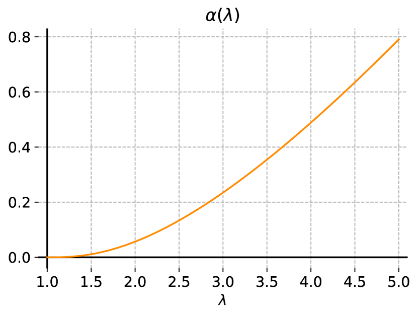

The asymptotic result from theorem 6.1 can be also refined and explicitly stated inside the critical window.
Theorem 6.3.
Let , denote the zero of the Airy function of smallest absolute value, and let denote the function
Then, the probability that a random multidigraph is acyclic satisfies the following asymptotic formula as :
Proof.
We follow the same steps as in the proof of theorem 6.1. Recall that, according to proposition 3.18, the probability we are interested in is
and we set
First result. We start by proving a weaker version of the first result, adding the assumption for some small enough positive . During the proof of the second part, we will be able to complete the full range of as . We apply Part (a) of lemma 5.3 with , , , and to conclude.
Second result. The result follows directly from Part (b) of lemma 5.3. In the first result, we could assume as small as wanted, so let us fix in . Observe that the range of of this second result overlaps with the first result (take, for example, for any ). We deduce, for in this intersection,
Since the function does not depend on , we can conclude that as . This completes the proof of the first result of the theorem.
Third result. We follow the same proof as for the case of theorem 6.1, arriving at the conclusion that is the sum of the two terms given in eqs. 6.1 and 6.2, and recalled here for convenience:
Since converges to , the term converges to
The two exponential terms differ in that . Since tends to infinity, the second term is negligible compared to the first one. We conclude
Using , we obtain
and
Plugging in those two approximations in the previous asymptotics, we conclude that
∎
Remark 6.4.
Note that if , where , then by applying theorem 6.1 one obtains again as . In the case when faster than , the supercritical case of theorem 6.1 is again applicable, although the asymptotic formula takes a different form if expressed in terms of due to appearance of additional terms in the Taylor expansion in the exponent. fig. 15 illustrates the result by plotting the limiting probabilities inside the critical window for .
6.2 Asymptotics of elementary digraphs and complex components
The next step after having the asymptotics of directed acyclic graphs is to express the probability that a random digraph or a multidigraph is elementary (all strong components are single vertices or cycles).
Theorem 6.5.
Let . The probability that a random multidigraph is elementary is
where is the zero of the derivative of the Airy function with the smallest modulus, , the constants and are as in theorem 6.1, and
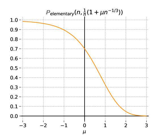
Proof.
According to proposition 3.18, the probability that a random multidigraph is elementary is given by
We let from now on.
Case . The result is a direct application of Part (a) of lemma 5.3 with , , , so .
Case . The result is a direct application of Part (b) of lemma 5.3.
Case . Let denote the roots of . It is known that they are all negative and distinct. Consider such that and define . Let denote the solution of the equation that is the -th closest to . Then, according to theorem 4.14, for any small enough , we have . Thus, by taking for the contour of integration , the residue theorem implies
From theorem 4.14 we conclude that as , the first root of is simple. This allows for a simpler expression for the residue. We also use (5.4) of lemma 5.3 to estimate the integral on the right-hand side
Next, using theorem 4.14 to estimate and and Part (c) of lemma 4.9 to estimate , we obtain
∎
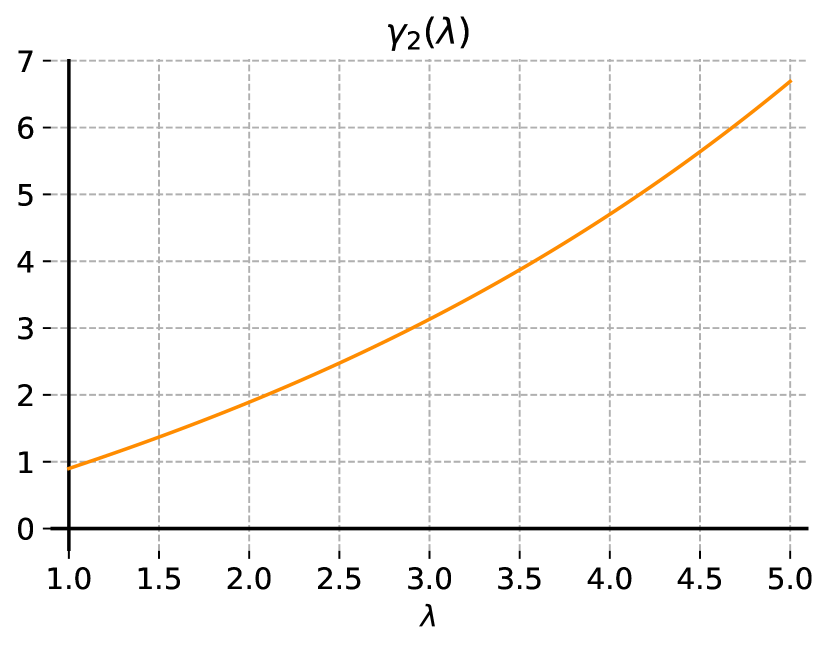
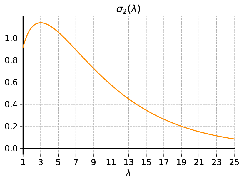
Remark 6.6.
Again, by comparing the critical case with and taking the limit of the supercritical case as , we observe that the answers have the same growth order , but there is again a discontinuity between , while . Again, when , the contour integral could be expressed as a sum of residues and we obtain for ,
where are the roots of sorted by their absolute values. As in remark 6.2, the first summand becomes dominant in the supercritical phase.
A similar analysis can reveal the probabilities that a digraph has a given ensemble of complex components, for example when there is exactly one complex component of excess whose kernel is cubic or has a deficiency (see lemma 3.12).
Theorem 6.7.
Let , . The probability that a random multidigraph sampled from has exactly one complex strong component and that this component has a given kernel of excess and deficiency (hence vertices and edges), satisfies
where the functions , are from theorem 6.1, is the zero of with the smallest modulus,
and
Proof.
According to proposition 3.18, the probability we are seeking is
As usual, we let in the following. We also denote by
the multi-graphic generating function of the multidigraph family under investigation.
Case . Direct application of Part (a) of lemma 5.3 with , , , , , , and therefore with .
Case . Direct application of Part (b) of lemma 5.3.
Case . Let denote the roots of , fix and set . Let us also write for , and denote by the th zero of , ordered by increasing modulus. Then theorem 4.14 implies that, as tends to , . Thus, expressing the coefficient extraction as a Cauchy integral and applying the residue theorem, we obtain
| (6.3) |
The second term is bounded using (5.4): from lemma 5.3
According to Taylor’s theorem, as ,
and
By constructing the Laurent series of the fraction and extracting the coefficient at of , we obtain
Let us gather some identities to simplify the numerator. We consider the point . theorem 4.14 implies and, using its very last statement, . The asymptotics of implies , so and . Part of lemma 4.9 is applied to approximate , and . theorem 4.14 is applied to approximate . Note that under this approximation, we also have . The numerator of the residue simplifies into
and eq. 6.3 becomes
The error term is negligible compared to the first summand, and we obtain
∎
Remark 6.8.
It may seem at first glance that the growth order of the supercritical probability receives an additional factor compared to the respective critical phase, when . However, if one develops the contour integral representing as a sum of residues, then the formula obtained by taking the first residue has the same growth rate as the limit of supercritical probability as . Indeed, as the contour integral contains a square of the function in the denominator, its zero is not a simple zero any longer, but a double one. Therefore, in order to extract the dominant residue, one has to take the cross-product of the derivatives of the numerator and the denominator, using the formula . It turns out that the derivative of with respect to gives an additional factor which then dominates the two other summands. This proves that the growth rates corresponding to the critical and the supercritical phases are identical.
Corollary 6.9.
Let , . The probability that one component of a random multidigraph sampled from is complex and bicyclic is
| (6.4) |
Moreover, when , this probability is asymptotically equal to . The probability that the kernel of the complex component is not cubic is also at most .
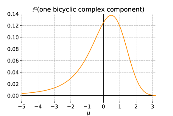
Another interesting phenomenon happens when for the case with one bicyclic complex component. If we expand the contour integral into an infinite sum of residues, each of the residues will be zero! However, by considering the residue at infinity, we can show that the integral takes a finite rational value.
Theorem 6.10.
The probability that a random multidigraph has one bicyclic complex component is asymptotically equal to .
Proof.
According to corollary 6.9, we need to evaluate the contour integral at . First of all, we can replace the arguments of the generalised Airy functions in (6.4) by , because the generalised Airy function is even on the imaginary axis. Then, the zeroes of the denominator are —the zeroes of the derivative of the Airy function. Let us calculate the residues at each of these zeros.
By expanding the Taylor series of the numerator and denominator, and taking the cross-product, we obtain
Next, we can use the linear relation (4.4) to obtain
| (6.5) |
By putting , the term vanishes and it turns out that each of the residues becomes zero.
In order to evaluate the integral, we compute the indefinite integral explicitly, and then substitute the endpoints. As pointed out in [HR68], , and by comparing it with [OLBC10, (9.10.2)], we obtain
where is the Scorer function satisfying
| (6.6) |
If is the second solution of the Airy equation, we can use the Wronskian formula [OLBC10, (9.2.7)]
and therefore deduce, using (6.5), that
This gives us the explicit antiderivative of the integrand expression.
In order to compute the corresponding definite integral, we need to find the limiting values of the antiderivative at the imaginary infinity. Note that, according to the derivative of the integral representation (6.6), the function is bounded on the imaginary axis by . At the same time, the limits of and at the imaginary infinity are (see [OLBC10, (9.7.10),(9.7.12)])
Consequently,
This implies
and finishes the proof. ∎
Remark 6.11.
Definite integrals involving Airy functions have been studied by many authors since at least 1966 [Asp66]. Using the Wronskian of the Airy function and the second solution of the Airy equation , Albright and Gavathas [AG86] presented a systematic way to compute indefinite integrals of the form
This includes, as a particular case, the integral , which is also mentioned in a paper of Knessl [Kne00] in the context of reflected Brownian motions with drift.
We expect that such integrals of generalised Airy functions could be probably of interest to a broader community of researchers in the context of mathematical physics, stochastic processes and queueing theory. As an example, in the paper of Knessl [Kne00] the parameters of interest are expressed in terms of integrals of Airy functions. In later papers by Janson [Jan13] and others [JLML10], a Brownian motion with parabolic drift is considered as well. The expected location of its maximum (and the moments) turn out to be expressible in terms of integrals of Airy functions. Interestingly, Brownian motion with parabolic drift appears in a different context, namely the study of critical digraphs, in a recent paper by Goldschmidt and Stephenson [GS21]. Taking into account that the expression provided by Knessl [Kne00, (3.8), Theorem 3] is very much reminiscent of the expressions we obtain for critical probabilities, we expect that the Airy integrals might provide an additional link reinforcing the quantitative study of the scaling limits of directed graphs from the Brownian viewpoint.
Below, in section 8, we provide accurate numerical values of the first several Airy integrals, the necessary constants for the supercritical case for the first several terms, and the figures representing the graphs of the Airy integrals proportional to the critical probability distribution functions .
7 Asymptotics of simple digraph families
We started our analysis with multidigraphs, in the previous section, because the calculations were slightly simpler compared to digraphs. We follow the same proofs as in section 6, applying the results from section 5.2 to replace those of section 5.1. It is instructive to see how the model choice affects the asymptotics.
7.1 Asymptotics of acyclic digraphs
Now, we can state the results on the probability that a random digraph is acyclic when , and . These theorems are handled with the same techniques as in the previous section by means of lemmas 5.4 and 5.5. As we can see below, results are roughly the same as in the case of multidigraphs except that models of digraphs involve some additional factor due to forbidden configurations.
Theorem 7.1.
Let , fixed. Then, the probability that a random simple digraph is acyclic satisfies the following asymptotic formulas as :
where
and the functions , are the same as given in theorem 6.1, and is the same as given in theorem 6.3.
Proof.
The proof is mainly the same as in theorem 6.1. According to proposition 3.19, the probability that a random simple digraph is acyclic is given by
where corresponds to the statement for the model, and for the model.
Case . We apply Part (a) of lemma 5.5 with , so that , and obtain
Case . We apply Part (b) of lemma 5.5 to obtain
Case . By taking the same contour of integration as in the proof of theorem 6.1, the residue theorem gives
Then lemma 5.5 implies
Next, by means of asymptotic formulas for and in corollary 4.13 and in corollary 4.10, and by letting , we obtain, with the help of a computer algebra system,
| (7.1) | ||||
| (7.2) |
where the constant is precisely as given in theorem 7.1, and are precisely as given in theorem 6.1. Choosing in the same way as in theorem 6.1, the right-hand side of (7.1) is indeed the main term of The statement of the theorem follows by setting for the model and for . ∎
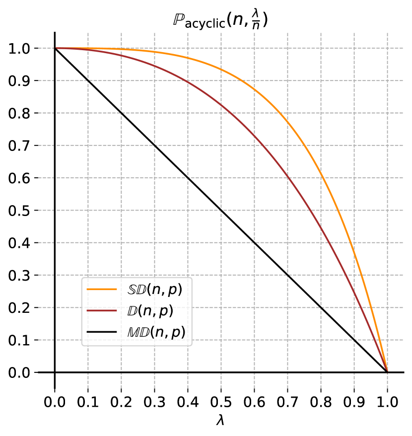
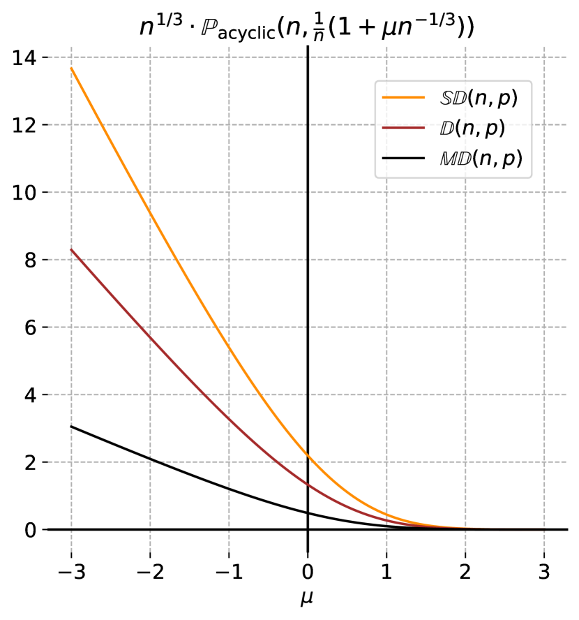
Corollary 7.2.
Let with going to infinity with . Then, the probability that a random digraph is acyclic satisfies the following asymptotic formula as :
where is the zero of the Airy function of smallest modulus and
Proof.
We follow the same proof as for theorem 6.3. As in the proof of the previous theorem, we start with the expression
First step. For going to with for some small enough positive , we apply Part (a) of lemma 5.5 with , so , and conclude
| (7.3) |
Second step. For with , we now apply Part (b) of lemma 5.5 to conclude, as in the previous theorem,
From Part (a) and (b) of theorem 6.3, since is independent of , we deduce that as tends to , we have . Thus, for going to with , we have
Since and , the asymptotic formula (7.3) obtained in the first step of the proof holds for any going to with .
Third step. Combining Part (b) and (c) of theorem 6.3, we deduce that as tends to infinity, we have
Combining this asymptotic formula with the second step, we conclude that when while , we have
∎
Remark 7.3.
As we have seen in remark 6.2 when and , the probability that or is acyclic can be expressed as a summation by expanding the contour integral. The results differ by a factor for and by for .
7.2 Asymptotics of elementary digraphs and complex components
The next step after having the asymptotics of directed acyclic graphs, is to express the probability that a random digraph is elementary or contains one complex component of a given excess. The following theorem expresses the probability that a random digraph is elementary when , and .
Theorem 7.4.
Let . The probability that a random simple digraph (resp. ) is elementary is
where is the zero of of smallest modulus, and
Proof.
According to proposition 3.19, the probability that a random digraph is elementary is given by
We notice that the analytic function satisfies the conditions of theorem 4.14, as it is entire and does not vanish on .
Case . We apply Part (a) of lemma 5.5 with so , , and are all equal to :
Case . We assume to be fixed or in a bounded real interval, and apply Part (b) of lemma 5.5 with . We obtain
We observe that for .
Case . We follow the same argument as in theorem 6.5 by using the residue theorem. The probability is asymptotically equivalent to
where is the solution to the equation that is the closest to zero. By plugging in the expressions for and from corollary 4.16, we obtain
∎
Remark 7.5.
In [dPD20] it was proven that as , the probability that a random digraph is elementary can be further refined as
This result was derived for the model of simple digraphs in the model , and can be deduced similarly for digraphs in the model as well. In principle, with an even more refined analysis, a complete asymptotic expansion in powers of could be obtained as well, and it can be shown that the coefficients of this expansion are identical for all the models considered in section 2.
By further analysis of the asymptotic probability of the presence of a complex component with given excess, it can be seen that when , the asymptotic probability that a digraph has one bicyclic complex component is . These two probabilities sum up to one if two terms of the asymptotic expansion are taken into account: , leaving an error of order .
Theorem 7.6.
Let , . The probability that a random digraph in the model or has exactly one complex strong component and that the excess of this component is satisfies
where the functions , are from theorem 6.1, is the zero of with the smallest modulus, from theorem 6.7,
and
and are defined in lemma 3.12 and computable using remark 3.13. In particular, a singularity analysis for fixed gives , where is given in lemma 3.12.
Proof.
We follow the same structure as in the proof of theorem 6.7. We defined and in lemma 3.12 so that the exponential generating functions of strongly connected simple digraphs of excess and strongly connected strict digraphs of excess are, respectively
Let denote the graphic generating function of digraphs containing exactly one strongly connected component of excess , while the others are single vertices or cycles of length . Let also . According to lemma 3.16, we have
| (7.4) |
where and , and .
In the rest of the proof, we restrict our attention to simple digraphs. The case of strict digraphs can be obtained in a straightforward manner. We want to compute the probability
| (7.5) |
Case . We apply Part (a) of lemma 5.5 by setting
so, in the notation of this lemma, , , , and . This implies and we obtain
Case . Part (b) of lemma 5.5 is applied with the previous parameters.
Case . Let denote the roots of , fix and set . Let us also write for , and denote by the th solution of , ordered by increasing modulus. Then corollary 4.16 implies that, as tends to , . Thus, expressing the coefficient extraction as a Cauchy integral and applying the residue theorem, we obtain
The second term is bounded using Part (c) of lemma 5.5:
| (7.6) |
Taylor’s theorem is applied to at , then the Laurent series of
is constructed and the residue at is computed as
We apply corollary 4.16 to approximate and the derivatives of and at . We apply Part (c) of corollary 4.10 to approximate and at and . The asymptotics of the residue and the error term are simplified using a computer algebra system. The error term from (7.6) is negligible and the asymptotics of the residue provide the statement of the theorem. ∎
Remark 7.7.
According to the exponential generating function of bicycles from lemma 3.16, corollary 6.9 holds for both and . In these cases, the constant is . Hence, the probability that or has one bicyclic complex component is asymptotically equal to .
8 Numerical results
In this section we provide numerical values for the probability that a random digraph (simple or multi-) with vertices and parameter belongs to a given family for different values of and . This is accomplished by computing the coefficients of the generating functions. We explore empirically how fast they tend to their respective limiting values. We also provide numerical values for the new special functions that we introduced in the form of Airy integrals.
8.1 Airy integrals
We start by providing a table of numerical values of Airy integrals of the form appearing in theorem 6.7. Let
The first few values of corresponding to different negative values of and integer values of , and also several values of , where is the dominant root of the derivative of the Airy function, are given in tables 2 and 3.
| 0 | 0.53566 66560 | 0.60833 46108 | 0.78025 12697 | 1.04871 55827 | 1.43382 48189 |
|---|---|---|---|---|---|
| 1 | 0.80907 32963 | 0.18173 76482 | 0.29442 48000 | 0.51700 82249 | 0.93651 41410 |
| 2 | 0.82428 81878 | 5.30647 07 | 0.10665 46071 | 0.23667 55204 | 0.53903 08295 |
| 3 | 0.68771 27402 | 1.51748 85 | 3.72902 31 | 0.10211 30475 | 0.28327 71366 |
| 4 | 0.50324 67342 | 4.25661 62 | 1.26360 41 | 4.19423 86 | 0.13868 39970 |
| 5 | 0.33424 30589 | 1.17273 42 | 4.16331 71 | 1.65168 25 | 6.40797 49 |
| 6 | 0.20565 74439 | 3.17750 22 | 1.33725 97 | 6.26910 09 | 2.81950 38 |
| 7 | 0.11879 14841 | 8.47523 11 | 4.19653 25 | 2.30288 09 | 1.18914 35 |
| 8 | 6.50381 41 | 2.22706 27 | 1.28898 06 | 8.21386 92 | 4.83151 22 |
| 9 | 3.39885 81 | 5.77144 16 | 3.88113 77 | 2.85229 69 | 1.89861 70 |
| 10 | 1.70465 23 | 1.47285 31 | 1.14711 18 | 9.66439 06 | 7.23897 30 |
| 0 | 1.71175 17513 | 1.18977 74561 | 0.24108 61434 | 5.93679 28 | 6.86168 24 |
|---|---|---|---|---|---|
| 1 | 1.43728 66407 | 1.19994 59529 | 0.27300 07028 | 7.21364 85 | 8.71568 73 |
| 2 | 1.00000 00000 | 0.95171 34841 | 0.23452 58919 | 6.49354 09 | 8.07052 10 |
| 3 | 0.61548 95913 | 0.65239 09401 | 0.17163 35341 | 4.93680 60 | 6.27592 36 |
| 4 | 0.34611 79347 | 0.40319 77130 | 0.11237 21118 | 3.34254 42 | 4.33391 88 |
| 5 | 0.18124 38129 | 0.23001 35204 | 6.75809 67 | 2.07309 81 | 2.73680 17 |
| 6 | 8.94935 23 | 0.12295 49383 | 3.79527 70 | 1.19839 99 | 1.60897 45 |
| 7 | 4.20355 45 | 6.22242 32 | 2.01266 66 | 6.53278 00 | 8.91294 64 |
| 8 | 1.89047 15 | 3.00370 59 | 1.01604 43 | 3.38662 88 | 4.69243 93 |
| 9 | 8.18150 40 | 1.39096 40 | 4.91269 11 | 1.68015 59 | 2.36312 51 |
| 10 | 3.42087 90 | 6.20709 94 | 2.28591 84 | 8.01635 84 | 1.14409 39 |
We provide the plots for for the functions with in fig. 16. Note that the value corresponds to the plot in fig. 13, which provides the remaining numbers for theorem 6.7 when . All the figures represent bell-shaped curves whose maxima lie in the interval . We rescale the plots by because this scaling factor also enters the final probabilities in theorem 6.7.
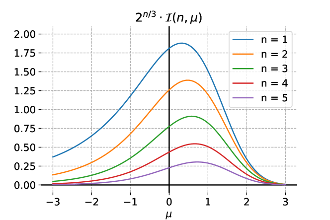
8.2 Empirical probabilities within the critical window
As the theorems in section 6 provide only the limiting values, with an error term of order when is bounded, it is interesting to track down how quickly the empirical probabilities for concrete values of and in the model converge to their limiting values. These values (for small values of and for inside the critical window) are given in tables 4, 5 and 6.
It is also interesting to compare the analogous convergence for the case of simple digraphs, depending on whether 2-cycles are allowed or not. The numerical results for the probabilities that a digraph is elementary (inside the centre of the critical window, i.e., when ) are given in table 7 for small values of .
| 100 | 3.00671 | 2.03423 | 1.14068 | 0.46304 | 0.11671 | 0.01642 | 0.00124 |
|---|---|---|---|---|---|---|---|
| 1000 | 3.02522 | 2.06335 | 1.17410 | 0.47705 | 0.10793 | 0.01012 | 0.00030 |
| 3000 | 3.03190 | 2.07219 | 1.18326 | 0.48068 | 0.10527 | 0.00859 | 0.00018 |
| 5000 | 3.03442 | 2.07542 | 1.18652 | 0.48196 | 0.10430 | 0.00807 | 0.00014 |
| 10000 | 3.03733 | 2.07906 | 1.19017 | 0.48337 | 0.10319 | 0.00751 | 0.00011 |
| 3.04943 | 2.09362 | 1.20431 | 0.48873 | 0.09876 | 0.00550 | 0.00004 |
| 100 | 0.99782 | 0.98513 | 0.92149 | 0.71322 | 0.36692 | 0.10522 | 0.01574 |
|---|---|---|---|---|---|---|---|
| 1000 | 0.99216 | 0.97411 | 0.90794 | 0.70645 | 0.34684 | 0.07442 | 0.00511 |
| 3000 | 0.99020 | 0.97095 | 0.90435 | 0.70446 | 0.34077 | 0.06604 | 0.00333 |
| 5000 | 0.98947 | 0.96981 | 0.90308 | 0.70374 | 0.33854 | 0.06307 | 0.00280 |
| 10000 | 0.98863 | 0.96854 | 0.90167 | 0.70293 | 0.33601 | 0.05979 | 0.00229 |
| 0.98521 | 0.96354 | 0.89622 | 0.69968 | 0.32582 | 0.04740 | 0.00089 |
| 100 | 0.00213 | 0.01360 | 0.05777 | 0.13535 | 0.14434 | 0.06652 | 0.01378 |
|---|---|---|---|---|---|---|---|
| 1000 | 0.00741 | 0.02231 | 0.06352 | 0.12980 | 0.13073 | 0.04610 | 0.00448 |
| 3000 | 0.00914 | 0.02459 | 0.06481 | 0.12833 | 0.12712 | 0.04081 | 0.00293 |
| 5000 | 0.00978 | 0.02539 | 0.06525 | 0.12781 | 0.12585 | 0.03897 | 0.00248 |
| 10000 | 0.01049 | 0.02627 | 0.06571 | 0.12723 | 0.12443 | 0.03693 | 0.00203 |
| 0.01333 | 0.02958 | 0.06737 | 0.12500 | 0.11896 | 0.02931 | 0.00081 |
| 100 | 0.777319 | 0.743468 | 0.713229 |
|---|---|---|---|
| 1000 | 0.724241 | 0.714032 | 0.706451 |
| 3000 | 0.713629 | 0.708269 | 0.704469 |
| 5000 | 0.710426 | 0.706492 | 0.703748 |
| 10000 | 0.707258 | 0.704693 | 0.702935 |
| 0.699687 | 0.699687 | 0.699687 |
8.3 Convergence outside the critical window
In this section we analyse the ratio of the empirical probability and the theoretical prediction when when are different fixed values separated from , and is large. We are dealing with all the three models , and . For each of the models, we are dealing with three different families: directed acyclic digraphs, elementary digraphs, and digraphs having one bicyclic complex component. Furthermore, for each of the families, we consider the subcritical case and . In total, this gives cases. For each of the 18 cases we compute the ratios of the empirical and theoretical probabilities and demonstrate their convergence to 1 by using log-log scale plots. These results are presented in table 8.
When , we expect that , while for we expect this difference to converge as . The constant in the error term is a function of . If this convergence takes place, then the values on the y-axis
will be approximated by decreasing linear functions when is large enough, with a slope for and for . The sign of the difference is empirically observed to be positive or negative, depending on the model, which is reflected when labelling the y-axis.
Although we observe nearly parallel decreasing lines for all our plots, the absolute value of the difference is higher for some models. This difference is most clearly seen, for example, in the supercritical case for digraphs with one bicyclic complex component, where in the multidigraph model we have the log-error of order for and , while this error raises to in the model and further to for the model .
![[Uncaptioned image]](/html/2009.12127/assets/x10.png) |
![[Uncaptioned image]](/html/2009.12127/assets/x11.png) |
![[Uncaptioned image]](/html/2009.12127/assets/x12.png) |
![[Uncaptioned image]](/html/2009.12127/assets/x13.png) |
![[Uncaptioned image]](/html/2009.12127/assets/x14.png) |
![[Uncaptioned image]](/html/2009.12127/assets/x15.png) |
![[Uncaptioned image]](/html/2009.12127/assets/x16.png) |
![[Uncaptioned image]](/html/2009.12127/assets/x17.png) |
![[Uncaptioned image]](/html/2009.12127/assets/x18.png) |
![[Uncaptioned image]](/html/2009.12127/assets/x19.png) |
![[Uncaptioned image]](/html/2009.12127/assets/x20.png) |
![[Uncaptioned image]](/html/2009.12127/assets/x21.png) |
![[Uncaptioned image]](/html/2009.12127/assets/x22.png) |
![[Uncaptioned image]](/html/2009.12127/assets/x23.png) |
![[Uncaptioned image]](/html/2009.12127/assets/x24.png) |
![[Uncaptioned image]](/html/2009.12127/assets/x25.png) |
![[Uncaptioned image]](/html/2009.12127/assets/x26.png) |
![[Uncaptioned image]](/html/2009.12127/assets/x27.png) |
9 Discussion and open problems
As the reader may have observed, the method that we develop in the current paper opens lots of possibilities to study various families of digraph models. Note that while all the analysis is carried out for , i.e., when every edge is chosen independently, a similar analysis for the model (with a fixed number of edges) can be carried out as well. In the latter case, the generating functions become bivariate, and one needs to extract the coefficient in the form . An example of such an analysis has been performed in a previous paper of the first two authors [dPD20] in the case of simple digraphs where 2-cycles are allowed. Their tools are equally applicable to the case of multidigraphs. In that previous paper, a different tool was used, which we refer to as graph decomposition: the graphic generating functions of DAGs and elementary digraphs could be expressed in terms of (derivatives) of the generating function of graphs. Nevertheless, it is possible to avoid the limitations of the graph decomposition method, and employ the double saddle point method with respect to the two variables.
The asymptotic behaviour of the models and should essentially be the same if the average number of edges in is relatively close to the number of edges , which means . The same remak holds for and , and . For the undirected version, such relationships are indicated in [ER60] (see also [Bol01, chap. II]) about the binomial model and the uniform model .
Many alternative graph and digraph models have recently gained more popularity, including models with degree constraints and with skewed degree distributions. The most typical type of degree distribution that occurs in real-world applications is the power-law. It is therefore tempting to extend the study of digraphs to the case where the in- and out-degrees are constrained, and belong to two dedicated sets (possibly with weights).
The classical models also have much more yet to study, including the joint distribution of the parameters in the source-like and sink-like components, the size of the giant strongly connected component, the distribution of the excess of the complex component, and so on. Using the symbolic method that we present in section 3, it is possible to tackle all these questions. Note that, however, in some cases, new analytic tools still need to be obtained. As a closely related question, since we expect that the excess of the strongly connected component is growing when is growing, should it mean that the maximum point of the bell-shaped curve in fig. 16 moves towards the right as the index of the Airy integral increases? Can it be shown that the bell-shaped curve, when centred, is Gaussian in the limit?
Some of the questions that may arise when one thinks of the limiting distributions in directed graphs, can be readily attacked with the tools that we already have in section 4. For example, if we are interested to know the probability that there are two complex components with given excesses (or three or more), we need to proceed with the coefficient extraction from a generating function in which there is an allowed family of complex components, each marked with a separate marking variable. The asymptotic analysis of such expressions results in more complicated Airy integrals of the form
Another model that also deserves to be studied is the model of directed hypergraphs, for which a variant of the symbolic method has been recently obtained in [RR20].
As we observe empirically in section 8, in order to have more precise computations for given and for the probabilities that a digraph belongs to a given family, one needs more terms in the asymptotic expansion, as the first error term is of order . Full asymptotic expansions (different for the models of multidigraphs and simple digraphs) could be useful in this context. For moderate values of (e.g. ), the error of the approximation in the supercritical phase could reach , but it eventually converges when grows. This means that there is a need for several different kinds of full asymptotic expansions, each for a different regime.
There is an intriguing similarity between the Airy integrals that appear in the current paper, and Airy integrals that appear in the study of the probability density function of a reflected Brownian motion with positive parabolic drift. To give an example, in Knessl’s paper [Kne00, (3.8)], an expression
arises as a solution to the system of partial differential equations
where denotes for any given time the probability density function with respect to particle position of a positive reflected Brownian motion starting at with drift at time . Remarkably, when , we obtain the rescaled asymptotic probability of directed acyclic graphs times , so in fact, .
As we argue in remark 6.11, this similarity may potentially lead to another link between the study of graphs and directed graphs and Brownian motions, originating from the paper of Aldous [Ald97] and first applied to the model of directed graphs in [GS21]. In [Jan13], Janson also links various Airy integrals to the moments of the time when a Brownian motion with parabolic drift attains its maximum.
Acknowledgements.
Vlady Ravelomanana once asked the question why the convolution product of generating functions was mostly concerned with disjoint components, and why there was seemingly no attempt to track allowed/forbidden edges between the distinct components. This simple idea has grown into the discovery of the symbolic method for directed graphs (which, as discovered later, has been independently established around 50 years ago by Liskovets, Robinson and then continued by Stanley and Gessel). Vlady also put in contact our two mini-groups who were working independently on the problem of digraph asymptotics, which allowed us to join our techniques and extend them. The authors are infinitely grateful to him for his inspiration and passion with random graphs and their variations.
Many interesting remarks have arisen during the seminar talks and discussions on various occasions, so we would like to thank Cyril Banderier, Christina Goldschmidt, Valeriy Liskovets and Andrea Sportiello, for their interest and their witty observations.
Sergey Dovgal was partially supported by the HÉRA project, funded by The French National Research Agency, grant no.: ANR-18-CE25-0002, and by the EIPHI Graduate School (contract ANR-17-EURE-0002), FEDER and Région Bourgogne Franche-Comté. Élie de Panafieu was supported by the Rise project RandNET, grant no.: H2020-EU.1.3.3 and the Lincs (www.lincs.fr). Dimbinaina Ralaivaosaona was supported by the National Research Foundation of South Africa, grant no.: 129413. Stephan Wagner was supported by the Knut and Alice Wallenberg Foundation, grant number KAW 2017.0112.
References
- [AG86] J. R. Albright and E. P. Gavathas. Integrals involving Airy functions. J. Phys. A, 19(13):2663–2665, 1986.
- [Ald97] D. Aldous. Brownian excursions, critical random graphs and the multiplicative coalescent. Ann. Probab., 25(2):812–854, 1997.
- [Asp66] D. E. Aspnes. Electric-field effects on optical absorption near thresholds in solids. Phys. Rev., 147(2):554–566, 1966.
- [Bal85] P. Baldwin. Zeros of generalized Airy functions. Mathematika, 32(1):104–117, 1985.
- [BFSS01] C. Banderier, P. Flajolet, G. Schaeffer, and M. Soria. Random maps, coalescing saddles, singularity analysis, and Airy phenomena. Random Structures Algorithms, 19(3-4):194–246, 2001.
- [BGJ12] M. Bloznelis, F. Götze, and J. Jaworski. Birth of a strongly connected giant in an inhomogeneous random digraph. J. Appl. Probab., 49(3):601–611, 2012.
- [BLL98] F. Bergeron, G. Labelle, and P. Leroux. Combinatorial species and tree-like structures, volume 67 of Encyclopedia of Mathematics and its Applications. Cambridge University Press, Cambridge, 1998.
- [Bol80] B. Bollobás. A probabilistic proof of an asymptotic formula for the number of labelled regular graphs. European Journal of Combinatorics, 1:311–316, 1980.
- [Bol01] B. Bollobás. Random graphs, volume 73 of Cambridge Studies in Advanced Mathematics. Cambridge University Press, Cambridge, second edition, 2001.
- [BR88] E. A. Bender and R. W. Robinson. The asymptotic number of acyclic digraphs. II. J. Combin. Theory Ser. B, 44(3):363–369, 1988.
- [BRRW86] E. A. Bender, L. B. Richmond, R. W. Robinson, and N. C. Wormald. The asymptotic number of acyclic digraphs. I. Combinatorica, 6(1):15–22, 1986.
- [CF04] C. Cooper and A. Frieze. The size of the largest strongly connected component of a random digraph with a given degree sequence. Combin. Probab. Comput., 13(3):319–337, 2004.
- [CFM94] C. Cooper, A. Frieze, and M. Molloy. Hamilton cycles in random regular digraphs. Combin. Probab. Comput., 3(1):39–49, 1994.
- [Cou19] M. Coulson. The critical window in random digraphs. Combin. Probab. Comput., pages 1–19, 2019.
- [dB81] N. G. de Bruijn. Asymptotic methods in analysis. Dover Publications, Inc., New York, third edition, 1981.
- [DdPR21] S. Dovgal, É. de Panafieu, and V. Ravelomanana. Exact enumeration of satisfiable 2-SAT formulae. arXiv preprint arXiv:2108.08067, 2021.
- [dP15] É. de Panafieu. Phase transition of random non-uniform hypergraphs. J. Discrete Algorithms, 31:26–39, 2015.
- [dP19] É. de Panafieu. Analytic combinatorics of connected graphs. Random Structures Algorithms, 55(2):427–495, 2019.
- [dPD19] É. de Panafieu and S. Dovgal. Symbolic method and directed graph enumeration. Acta Math. Univ. Comenian. (N.S.), 88(3):989–996, 2019.
- [dPD20] É. de Panafieu and S. Dovgal. Counting directed acyclic and elementary digraphs. Sém. Lothar. Combin., 84B:Art. 2, 12 pages, 2020.
- [DR11] H. Daudé and V. Ravelomanana. Random 2 XORSAT phase transition. Algorithmica, 59(1):48–65, 2011.
- [ER59] P. Erdős and A. Rényi. On random graphs. I. Publ. Math. Debrecen, 6:290–297, 1959.
- [ER60] P. Erdős and A. Rényi. On the evolution of random graphs. Magyar Tud. Akad. Mat. Kutató Int. Közl., 5:17–61, 1960.
- [ER61] P. Erdős and A. Rényi. On the strength of connectedness of a random graph. Acta Math. Acad. Sci. Hungar., 12:261–267, 1961.
- [ER66] P. Erdős and A. Rényi. On the existence of a factor of degree one of a connected random graph. Acta Math. Acad. Sci. Hungar., 17:359–368, 1966.
- [FK16] A. Frieze and M. Karoński. Introduction to random graphs. Cambridge University Press, Cambridge, 2016.
- [FKL17] A. Ferber, G. Kronenberg, and E. Long. Packing, counting and covering Hamilton cycles in random directed graphs. Israel J. Math., 220(1):57–87, 2017.
- [FKP89] P. Flajolet, D. E. Knuth, and B. Pittel. The first cycles in an evolving graph. Discrete Math., 75(1-3):167–215, 1989.
- [FNN+17] A. Ferber, R. Nenadov, A. Noever, U. Peter, and N. Škorić. Robust Hamiltonicity of random directed graphs. J. Combin. Theory Ser. B, 126:1–23, 2017.
- [FS09] P. Flajolet and R. Sedgewick. Analytic combinatorics. Cambridge University Press, Cambridge, 2009.
- [FSS04] P. Flajolet, B. Salvy, and G. Schaeffer. Airy phenomena and analytic combinatorics of connected graphs. Electron. J. Combin., 11(1):Research Paper 34, 30 pages, 2004.
- [Ges96] I. M. Gessel. Counting acyclic digraphs by sources and sinks. Discrete Math., 160(1-3):253–258, 1996.
- [Gil59] E. N. Gilbert. Random graphs. Ann. Math. Statist., 30:1141–1144, 1959.
- [Gro54] D. Grohne. Über das Spektrum bei Eigenschwingungen ebener Laminarströmungen. Z. Angew. Math. Mech., 34:344–357, 1954.
- [GS05] P. J. Grabner and B. Steinsky. Asymptotic behaviour of the poles of a special generating function for acyclic digraphs. Aequationes Math., 70(3):268–278, 2005.
- [GS21] C. Goldschmidt and R. Stephenson. The scaling limit of a critical random directed graph. arXiv:1905.05397v3 [math.PR], 2021. Preprint.
- [HR68] T. H. Hughes and W. H. Reid. The stability of spiral flow between rotating cylinders. Philos. Trans. R. Soc. Lond. Ser. A Math. Phys. Eng. Sci., 263(1135):57–91, 1968.
- [HSS16] D. Hefetz, A. Steger, and B. Sudakov. Random directed graphs are robustly Hamiltonian. Random Structures Algorithms, 49(2):345–362, 2016.
- [Jan13] S. Janson. Moments of the location of the maximum of Brownian motion with parabolic drift. Electron. Commun. Probab., 18:no. 15, 8 pages, 2013.
- [JKŁP93] S. Janson, D. E. Knuth, T. Łuczak, and B. Pittel. The birth of the giant component. Random Structures Algorithms, 4(3):231–358, 1993.
- [JLML10] S. Janson, G. Louchard, and A. Martin-Löf. The maximum of Brownian motion with parabolic drift. Electron. J. Probab., 15:no. 61, 1893–1929, 2010.
- [JŁR00] S. Janson, T. Łuczak, and A. Ruciński. Random graphs. Wiley-Interscience Series in Discrete Mathematics and Optimization. Wiley-Interscience, New York, 2000.
- [Kar90] R. M. Karp. The transitive closure of a random digraph. Random Structures Algorithms, 1(1):73–93, 1990.
- [KLS13] M. Krivelevich, E. Lubetzky, and B. Sudakov. Longest cycles in sparse random digraphs. Random Structures Algorithms, 43(1):1–15, 2013.
- [Kne00] C. Knessl. Exact and asymptotic solutions to a PDE that arises in time-dependent queues. Adv. in Appl. Probab., 32(1):256–283, 2000.
- [Kol99] V. F. Kolchin. Random graphs, volume 53 of Encyclopedia of Mathematics and its Applications. Cambridge University Press, Cambridge, 1999.
- [KP89] D. E. Knuth and B. Pittel. A recurrence related to trees. Proc. Amer. Math. Soc., 105(2):335–349, 1989.
- [Lag83] E. N. Laguerre. Mémoire sur la théorie des équations numériques. J. Math. Pures Appl. (3), 9:99–146, 1883.
- [Lis69] V. A. Liskovets. A recurrent method for the enumeration of graphs with labelled vertices. Dokl. Akad. Nauk SSSR, 184(6):1284–1287, 1969.
- [Lis70] V. A. Liskovets. The number of strongly connected directed graphs. Math. Notes Acad. Sci. USSR, 8(6):877–882, 1970.
- [Lis73] V. A. Liskovets. A contribution to the enumeration of strongly connected digraphs. Dokl. Akad. Nauk BSSR, 17:1077–1080, 1973.
- [ŁS09] T. Łuczak and T. G. Seierstad. The critical behavior of random digraphs. Random Structures Algorithms, 35(3):271–293, 2009.
- [Łuc90] T. Łuczak. The phase transition in the evolution of random digraphs. J. Graph Theory, 14(2):217–223, 1990.
- [Mah40] K. Mahler. On a special functional equation. J. London Math. Soc., 15:115–123, 1940.
- [OLBC10] F. W. J. Olver, D. W. Lozier, R. F. Boisvert, and C. W. Clark, editors. NIST handbook of mathematical functions. Cambridge University Press, New York, NY, 2010.
- [Rob73] R. W. Robinson. Counting labeled acyclic digraphs. In New directions in the theory of graphs (Proc. Third Ann Arbor Conf., Univ. Michigan, Ann Arbor, Mich., 1971), pages 239–273, 1973.
- [Rob77] R. W. Robinson. Counting strong digraphs. J. Graph Theory, 1(2):189–190, 1977.
- [Rob95] R. W. Robinson. Counting digraphs with restrictions on the strong components. In Combinatorics and graph theory ’95, Vol. 1 (Hefei), pages 343–354. World Sci. Publ., River Edge, NJ, 1995.
- [RR20] V. Rasendrahasina and V. Ravelomanana. Generating functions of some families of directed uniform hypergraphs. Sém. Lothar. Combin., 84B:Art. 72, 11 pages, 2020.
- [RRW20] D. Ralaivaosaona, V. Rasendrahasina, and S. Wagner. On the probability that a random digraph is acyclic. In 31st International Conference on Probabilistic, Combinatorial and Asymptotic Methods for the Analysis of Algorithms, volume 159 of LIPIcs. Leibniz Int. Proc. Inform., pages Art. 25, 17 pages. Schloss Dagstuhl. Leibniz-Zent. Inform., Wadern, 2020.
- [Sok12] A. D. Sokal. The leading root of the partial theta function. Adv. Math., 229(5):2603–2621, 2012.
- [Sok13] A. D. Sokal. Some wonderful conjectures (but very few theorems) concerning the leading root of some formal power series, 2013. Combinatorics, Algebra, and More: A Conference in Celebration of Peter Cameron.
- [SP14] J. Schur and G. Pólya. Über zwei Arten von Faktorenfolgen in der Theorie der algebraischen Gleichungen. J. Reine Angew. Math., 144:89–113, 1914.
- [Sta73] R. P. Stanley. Acyclic orientations of graphs. Discrete Math., 5:171–178, 1973.
- [Ste70a] V. E. Stepanov. On the probability of connectedness of a random graph . Theory Probab. Appl., 15(1):55–67, 1970.
- [Ste70b] V. E. Stepanov. Phase transitions in random graphs. Theory Probab. Appl., 15(2):187–203, 1970.
- [Ste73] V. E. Stepanov. Structure of the random graphs . Theory Probab. Appl., 17(2):227–242, 1973.
- [vdH17] R. van der Hofstad. Random graphs and complex networks. Vol. 1. Cambridge Series in Statistical and Probabilistic Mathematics, 43. Cambridge University Press, Cambridge, 2017.
- [VS04] O. Vallée and M. Soares. Airy functions and applications to physics. Imperial College Press, London, 2004.
- [Wri71] E. M. Wright. The number of strong digraphs. Bull. London Math. Soc., 3:348–350, 1971.
- [Wri77] E. M. Wright. Formulae for the number of sparsely-edged strong labelled digraphs. Quart. J. Math. Oxford Ser. (2), 28(111):363–367, 1977.