Virtual Forward Dynamics Models for Cartesian Robot Control

Abstract

In industrial context, admittance control represents an important scheme in programming robots for interaction tasks with their environments. Those robots usually implement high-gain disturbance rejection on joint-level and hide direct access to the actuators behind velocity or position controlled interfaces. Using wrist force-torque sensors to add compliance to these systems, force-resolved control laws must map the control signals from Cartesian space to joint motion. Although forward dynamics algorithms would perfectly fit to that task description, their application to Cartesian robot control is not well researched. This paper proposes a general concept of virtual forward dynamics models for Cartesian robot control and investigates how the forward mapping behaves in comparison to well-established alternatives. Through decreasing the virtual system’s link masses in comparison to the end effector, the virtual system becomes linear in the operational space dynamics. Experiments focus on stability and manipulability, particularly in singular configurations. Our results show that through this trick, forward dynamics can combine both benefits of the Jacobian inverse and the Jacobian transpose and, in this regard, outperforms the Damped Least Squares method.

1 Introduction

In robotics, task space control is important for many applications, since it provides a natural way for programmers to specify goals and constraints. The according control laws can be formulated in operational space of the end-effector. Since the robots are articulated mechanisms and are powered in their joints, these controllers need to map the Cartesian control signals to the robots’ configurations space, i.e. the motor actuators. We will refer to matrices that accomplish this as mapping matrices. Two frequently-used variants of mapping matrices are the transpose of the manipulator’s Jacobian and its inverse.

The Jacobian transpose is an important part in many classes of control schemes for torque-actuated robots, such as in hybrid force/motion control Whitney1977 (1), Raibert1981 (2), Khatib1987 (3), parallel force/motion control Chiaverini1993 (4), and impedance control Hogan1985 (5), Villani2008 (6). In principal, the approaches use the Jacobian transpose as static relationship between end-effector wrenches and joint torques for controlling robots in contact with their environments. Although not strictly required, control performance is generally improved through decoupling robot dynamics in operational space Khatib1987 (3), prior to mapping the signals to joint space. In addition, there are also algorithmic solutions using the principle of inverse dynamics to compute suitable joint torques from motion control signals, e.g. with the Recursive Newton-Euler Algorithm (RNEA) Featherstone2008 (7).

An important subset of robots, however, does not provide joint interfaces on torque level. These systems are often found in industrial context, and are the primary focus of this paper. In Villani2008 (6), those systems are referred to as simplified systems because they hide internal dynamics decoupling behind a velocity interface. In this paper, we will refer to them as velocity-actuated systems to underline the type of interface exposed by the robot vendors. On these systems, velocity-resolved control variants, such as admittance control Villani2008 (6), usually leverage Jacobian inverse-related methods, such as the Damped Least Squares (DLS) Wampler1986 (8) as the mapping to joint space.

Unlike inverse dynamics for torque-actuated systems, literature on velocity-actuated robots mostly neglects forward dynamics as an algorithmic option for control. This is surprising, because it represents a straightforward mapping from Cartesian wrench space to joint accelerations. While we used this method to control robots in previous work Scherzinger2017 (9), Scherzinger2019Inverse (10), the new contribution of this paper is an in-depth analysis of particular features of this mapping and an evaluation against other well-established methods. The goal and novelty is a drop-in-replacement for the Jacobian inverse and DLS in controllers for velocity-actuated robots. Through using a dynamics-conditioned, virtual forward model, we match the linear, decoupled behavior of the Jacobian inverse while simultaneously keeping the inherent robustness in singularities of the Jacobian transpose method.

The paper is structured as follows: In 2 we briefly recapitulate the inverse kinematics mapping problem along with established methods to make it easy for the reader to follow comparisons in the experiments. Section 3 then presents forward dynamics-based mappings for Cartesian control. In the experiments section 4, we investigate ill conditioning, stability and manipulability in singular configurations and evaluate our approach against suitable subsets of the Jacobian Inverse, the Jacobian transpose and the DLS method. We finally discuss remaining points and suggestions in 5 and conclude with directions for further research in 6.

2 Problem statement and related work

The goal of this paper is to evaluate forward dynamics-based mappings against well-established methods. We use Singular Value Decomposition (SVD) as a tool to investigate the characteristics of the mapping matrices. SVD factorizes a matrix $\bm{M}$ according to

$$\bm{M}=\bm{U}\bm{\Sigma}\bm{V}^{T},\quad\text{with}~{}\sigma_{i}=\Sigma_{ii}.$$ (1)

$\bm{U}$ and $\bm{V}^{T}$ are orthogonal matrices. The entries $\sigma_{i}\geq 0$ of the diagonal matrix $\bm{\Sigma}$ are known as the singular values and determine the scale of the mapping. For our experiments, $\sigma_{\text{min}}$ and $\sigma_{\text{max}}$ as the minimal and maximal singular values are of particular interest in analyzing stability and manipulability.

To recapture some basic concepts, let the forward kinematics mapping be given with

$$\bm{x}=g\left(\bm{q}\right),$$ (2)

which computes an end-effector pose, denoted here with $\bm{x}$ from the joint state vector $\bm{q}$. The velocity vector of generalized coordinates $\dot{\bm{q}}$ maps with

$$\dot{\bm{x}}=\bm{J}\dot{\bm{q}}$$ (3)

to end effector velocity vector $\dot{\bm{x}}$, using the manipulator Jacobian $\bm{J}=\bm{J}(\bm{q})$. We generally omit the joint vector dependency in further notation for brevity reasons. For non-redundant manipulators, the inverse mapping is given by

$$\dot{\bm{q}}=\bm{J}^{-1}\dot{\bm{x}}~{}.$$ (4)

Near singular configurations, $\bm{J}$ looses rank, such that its inverse becomes numerically unstable. The respective mapping for end-effector forces and torques to joint space with

$$\bm{\tau}=\bm{J}^{T}\bm{f}$$ (5)

does not suffer from these instabilities. However, $\bm{J}$ becoming rank-deficient means that some components of $\bm{f}$ will lie in the nullspace of the Jacobian transpose, i.e. they will be balanced by the mechanism’s mechanics and will hence not be able to actuate the joints. This effect is a severe limitation for controller implementations.

Applied to motion control, a formal investigation of the Jacobian transpose method and a numerical solution to the Inverse Kinematics problem was presented in Wolovich1984 (11). The authors’ solution derives from a simple, 2nd order dynamical system

$$\ddot{\bm{q}}=\bm{K}\bm{J}^{T}\left(\bm{x}^{d}-g(\bm{q})\right)~{},$$ (6)

computing joint accelerations from the difference of a desired pose $\bm{x}^{d}$ and the current pose as determined by the forward kinematics $g(\bm{q})$. They show with a Lyapunov stability analysis that the system is asymptotically stable for an arbitrary positive definite matrix $\bm{K}$.

Using $\bm{J}^{T}$ will serve as a lower bound and baseline in stability considerations of our contribution.

The DLS method is an applications of the Levenberg-Marquardt stabilization to manipulator control Nakamura1986 (12), Wampler1986 (8) and tries to remove instabilities of $\bm{J}^{-1}$ near singular configurations. Note that the original version as proposed in Wampler1986 (8) uses partial velocity matrices, adding the benefit of allowing different reference frames for each element. Since we don’t make use of this feature, we replace it with the common manipulator Jacobian $\bm{J}$ instead. Similar to pseudo inverse methods for redundant systems, which minimize $\lVert\bm{J}\dot{\bm{q}}-\dot{\bm{x}}\rVert^{2}$, the idea is to add a damping term $\alpha$ against excessive joint velocities that will trade-off accuracy for stability near singular configurations with

$$\lVert\bm{J}\dot{\bm{q}}-\dot{\bm{x}}\rVert^{2}+\alpha^{2}\lVert\dot{\bm{q}}\rVert^{2}.$$ (7)

The solution that minimizes this quantity is given by

$$\dot{\bm{q}}=(\bm{J}^{T}\bm{J}+\alpha^{2}\bm{I})^{-1}\bm{J}^{T}\dot{\bm{x}},$$ (8)

see e.g. Buss2004 (13) for a derivation. The matrix $(\bm{J}^{T}\bm{J}+\alpha^{2}\bm{I})$ is non-singular, which can be shown with singular value decomposition Buss2004 (13) and hence is guaranteed to be invertible. This method is well established for practical control implementations and can serve as a drop-in replacement for $\bm{J}^{-1}$ in control loops. We use this method as a baseline to compare our new forward dynamics-based method in terms of manipulability.

A popular enhancement to DLS, using this method, is Selectively Damped Least Squares (SDLS) Buss2005 (14). The method converges faster and circumvents to choose a suitable $\alpha$ by introducing singular vector-specific damping terms of the singular value decomposition of $\bm{J}$ at the expense of a higher runtime cost.

Other methods include the more recent Exponentially Damped Least Squares (EDLS) Carmichael2017 (15), which is a solution with the focus on physical Human-Robot interaction (pHRI). Although effectively avoiding elbow-lock and wrist-lock among other common singular phenomena, it requires explicit, albeit easy parameterization by the user.

Both the Jacobian inverse and the Jacobian transpose have strengths and shortcomings and present mappings for physically different control spaces. When used on velocity-actuated systems, the Jacobian inverse does not need dynamic decoupling, but suffers from instability, which DLS effectively mitigates at the expense of loosing accuracy with increased damping. The Jacobian transpose needs dynamics decoupling in the controller, but offers inherent stability near singular configurations. A general incentive is to obtain the best of these corner cases. This paper proposes and empirically evaluates forward dynamics as a suitable approach to achieve this combination at the core of closed-loop control schemes.

3 Cartesian control with forward dynamics

3.1 Forward dynamics simulations

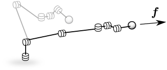
Figure 1: Illustration of pulling an exemplary robot manipulator into singularity.

To motivate the usage of forward dynamics in control applications let’s illustrate its behavior with a use case: Fig. 1 depicts an arbitrary manipulator with joints and links. Let’s assume that the joints are pure articulations without motors and are back-drivable, i.e. they can freely be moved. An external force $\bm{f}$ is pulling the mechanism into singularity, in which the mechanism yields the external forces as good as it can, limited by kinematic constraints. In the fully stretched case, increasing $\bm{f}$ will not create further motion. The robot’s mechanics compensate the external load until a possible breakage of the links. This behavior is in fact inverse to how $\bm{J}^{-1}$ would compute joint motion due to an external error vector, where theoretically infinite joint velocity would occur.

To make use of forward dynamics simulations, robotic manipulators can be modeled as a system of articulated, rigid bodies. The equations of motion describe the relationship between generalized loads $\bm{\tau}$ in the joints, external loads $\bm{f}$, acting on the end-effector and motion in generalized coordinates $\bm{q}$ with the following ordinary differential equations in symbolic matrix notation

$$\bm{\tau}+\bm{J}^{T}\bm{f}=\bm{H}({\bm{q}})\ddot{\bm{q}}+\bm{C}(\bm{q},\dot{\bm{q}})+\bm{G}(\bm{q})~{}.$$ (9)

$\bm{H}$ denotes the mechanism’s positive definite inertia matrix, $\bm{C}$ comprises the Coriolis and centrifugal terms and $\bm{G}$ is the vector of gravitational components. Forward dynamics computation has the goal of solving Eq. (9) for $\bm{q}(t)$, i.e. simulating the mechanism’s reaction motion through time, given external loads.

Literature has proposed several methods for forward dynamics computations, which can be categorized Featherstone2008 (7) as mainly belonging to inertia matrix methods with implementations of the composite rigid body algorithm, e.g. in McMillan1998 (16), Featherstone2005 (17), or the propagation methods with the articulated body algorithm Featherstone1983 (18) being an important representative. We refer the interested reader to Featherstone2008 (7) for an broad coverage of the field and recent implementation of various algorithms.

Forward dynamics is a substantial component in multi body simulations. The fact that it is, however, mainly neglected for closed-loop control on velocity-actuated systems may stem from the fact that computing good approximations for $\bm{H}$ and $\bm{C}$ of the robots is extremely difficult. The required crucial data, such as link masses and inertia tensors is hardly available in data sheets. On the other hand, a second reason for not being used might be that even if those data were available, the benefit of forward simulating highly realistic motion would get lost when executed on velocity-actuated systems. Their internal joint servos with high-gain disturbance rejection could not make use of the accuracy of dynamics that was used to generate that motion. The reference trajectory to follow would appear as any arbitrary trajectory.

This thought points to an interesting opportunity: We could reduce Eq. (9) to a rough simplification and investigate, if it’s possible to condition $\bm{H}$ to beneficially tweak the behavior of this mapping when using it as a forward model in closed-loop control.

3.2 A general closed-loop control

Figure 2: Closed-loop control with forward dynamics. We use a virtual system to forward simulate joint motion as a reference to the real robot.

To motivate simplifications to Eq. (9), we investigate how a controller would perceive the system in a possible closed loop control. A general scheme is shown in Fig. 2. A suitable control law computes a Cartesian control signal $\bm{f}^{c}$, using a user specified reference input and a controlled variable as feedback from the robot. Note the role of the virtual system as a forward model in the controller: We simulate how our proxy system behaves and send that as a reference to the real system. Since we obtain joint accelerations as a response from our forward model, we integrate those signals before sending them as reference to the real robot. The advantage is, that this virtual model will react kinematically and mechanically plausible to external loads $\bm{f}^{c}$, as was illustrated in Fig. 1.

From the control law’s point of view, a linear, virtual system would be beneficial for using constant control gains for wide regions of the robot’s joint configuration space. By dropping the gravity term ($\bm{G}(\bm{q})=\bm{0}$) from Eq. (9), we assure that the control law does not need to constantly compensate this virtual load. If we further consider instantaneous motion for each control cycle, i.e. accelerate from rest with $\dot{\bm{q}}=\bm{0}$, we can drop the non-linearities $\bm{C}(\bm{q},\dot{\bm{q}})$ and obtain

$$\ddot{\bm{q}}=\bm{H}^{-1}(\bm{q})\bm{J}^{T}\bm{f}^{c}~{}$$ (10)

as an unbiased forward mapping. We also set $\bm{\tau}\equiv\bm{0}$ to emphasize that $\bm{f}^{c}$ shall be the only virtual load guiding the virtual system.

While dropping these terms reduces computational complexity in our controller, including them can offer additional configuration. This is briefly discussed in section 5.

Note that $\bm{H}^{-1}(\bm{q})$ needs to be computed in each control cycle due to its dependency of the current joint state. In the experiments section, we evaluate computational cost in comparison to other mapping matrices. Since Eq. (10) is effectively a Jacobian transpose-based method, the next step is to decouple our virtual $\bm{H}^{-1}$.

3.3 Decoupling virtual dynamics

We start with the time derivative of Eq. (4)

$$\ddot{\bm{x}}=\dot{\bm{J}}\dot{\bm{q}}+\bm{J}\ddot{\bm{q}}~{}~{}$$ (11)

and consider instantaneous accelerations in each cycle while the virtual system is still at rest, so that $\dot{\bm{J}}\dot{\bm{q}}=\bm{0}$. With Eq. (10) we obtain

$$\ddot{\bm{x}}=\bm{J}\bm{H}^{-1}\bm{J}^{T}\bm{f}^{c}=\bm{\Lambda}^{-1}\bm{f}^{c}~{}~{},$$ (12)

which describes the Cartesian instantaneous acceleration of the virtual system due to the Cartesian control input $\bm{f}^{c}$. The quantity $\bm{\Lambda}$ is known as the mass matrix in operational space, see e.g. Khatib1987 (3), Villani2008 (6), with $\bm{\Lambda}=\bm{J}^{-T}\bm{H}\bm{J}^{-1}$.

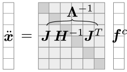
Figure 3: Graphical illustration of the mapping from wrench space to Cartesian acceleration. $\bm{\Lambda}$ is a $6\times 6$ matrix for both redundant and non-redundant systems. Our goal is to obtain a decoupled, diagonal mapping for arbitrary joint configurations.

The intention of our dynamic decoupling is to make $\bm{\Lambda}^{-1}$ a time-invariant, diagonal matrix across joint configurations $\bm{q}$. This ideal mapping is illustrated in Fig. 3. In order to preserve consistency of our virtual system and the real robot, we use identical kinematics for both systems. This ensures that the reference signals for the real robot to follow agree with possible limits. We are, however, free in changing the dynamics of the virtual $\bm{H}$ to obtain the desired effect, in particular its mass distribution. The Cartesian control signal $\bm{f}^{c}$ acts directly on the virtual mechanism’s end effector. If that end-effector link is dominant with respect to the overall dynamics, determined by the other links, we could obtain a behavior that comes close to an idealized unit mass. Fig. 4 illustrates this phenomenon.

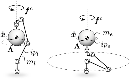
Figure 4: Dynamics-conditioned, virtual model for an exemplary robot. The goal is to make the mechanism behave as a unit mass, which is illustrated with the oversized sphere.

As a consequence, the overall systems’ center of mass roughly stays with the end-effector. Likewise does the operational space inertia $\bm{\Lambda}$ depend less on joint configurations, and $\bm{f}^{c}$ experiences the same rotational inertia for both configurations. Having a realistic link mass distribution would instead mean higher inertia with greater distance to the rotary axis. To measure the effect of end-effector mass dominance, we define

$$\gamma=\frac{m_{e}}{m_{l}}=\frac{ip_{e}}{ip_{l}}$$ (13)

to be the ratio of end-effector mass $m_{e}$ and link mass $m_{l}$. The quantities $ip_{e}$ and $ip_{l}$ denote the polar momentums of inertia of the end-effector and the other links, respectively. In the experiments section, we empirically show that increasing $\gamma$ in deed leads to the desired behavior and provides a decoupled virtual system for Cartesian closed-loop control.

3.4 Closed-loop stability

Comparison of Eq. (6) and Eq. (10) shows a strong resemblance of our forward dynamics-based approach with the dynamical system from Wolovich1984 (11), if $\bm{f}^{c}=\bm{x}^{d}-g(\bm{q})$. In Wolovich1984 (11), the authors prove with a Lyapunov stability analysis that a closed loop system, built from this mapping, is asymptotically stable for an arbitrary positive definite matrix $\bm{K}$. This formal proof also includes our proposed $\bm{H}^{-1}$, which is, due to being grounded in the manipulator’s kinetic energy $T=\dot{\bm{q}}^{T}\bm{H}\dot{\bm{q}}$, also positive definite.

4 Experiments and results

We evaluated our forward dynamics-based approach against the DLS and against the two corner cases $\bm{J}^{-1}$ and $\bm{J}^{T}$ in various experiments. We chose the Universal Robot UR10’s kinematics for our experiments. Our perception is that this robot is well-known and used both in industry and academia and therefore presents a suitable platform.

Depending on the phenomena investigated, a subset of different mapping matrices was used. An overview of these matrices and their composition is given in Fig. 5 along with the abbreviations used in the plots. We implemented each mapping matrix literally, i.e. as a multiplication of the respective symbols in C++, using the robot’s kinematics from a popular ROS Quigley2009 (19) package and the algorithms for computing $\bm{J}$ and $\bm{H}$ from a well-established robotics library.

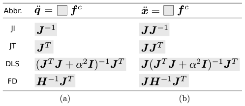
Figure 5: Mapping matrices for the experiments. The abbreviations stand for Jacobian inverse (JI), Jacobian transpose (JT), Damped Least Squares (DLS) and Forward Dynamics (FD). Two types are investigated: (a) Mappings from Cartesian space to joint space and (b) mappings from Cartesian space to Cartesian space.

For all experiments, the following values were chosen for the forward dynamics mappings:

$$m_{e}=$1\text{\,}\mathrm{k}\mathrm{g}$,\quad m_{l}=\frac{m_{e}}{\gamma},\quad ip_{e}=$1\text{\,}\mathrm{k}\mathrm{g}\mathrm{/}\mathrm{m}^{2}$,\quad ip_{l}=\frac{ip_{e}}{\gamma}$$ (14)

The ratio $\gamma$ was then varied according to the investigation of each experiment.

4.1 Decoupling

In this experiment, we evaluated the effectiveness of our virtual model dynamics decoupling and compared the mapping to both the Jacobian inverse and the Jacobian transpose as reference. The mapping matrices were of type (b) from Fig. 5.

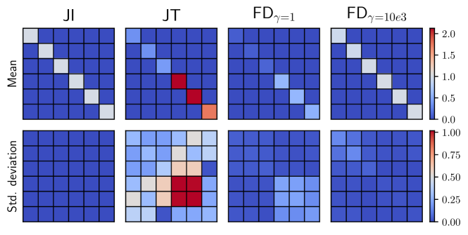
Figure 6: Analysis of the $6\times 6$ mapping matrices of type (b) from Fig. 5. The plot shows the individual matrix entries in form of 2d heat plots. To obtain the plots, we sampled $100.000$ random configurations of $\bm{q}$ uniformly with $q_{i}\in\left[-\pi,\pi\right]$ and computed the respective mapping matrix for each type. The figures show mean and standard deviation for the entirety of samples.

Fig. 6 shows the results of the analysis. All mean matrices are diagonal, which is to expect for sampling a vast amount of arbitrary joint configurations. The standard deviations, however, show a strong configuration dependency for the Jacobian transpose. This mapping would be suboptimal if used in a closed-loop control scheme. Instead, the Jacobian inverse behaves ideal and converges to the identity matrix. Note that using forward dynamics with an even mass distribution ($\gamma=1$) already improves upon the Jacobian transpose. The experiment further shows, that with a significant end-effector mass dominance ($\gamma=10e^{3}$) the forward dynamics mapping converges to the Jacobian inverse and makes this mapping particularly suitable for closed-loop control in terms of linearity.

4.2 Ill-conditioned configurations

In this experiment, we continued the evaluation of decoupling and compared FD and DLS with regard to ill conditioning of the mapping matrices from Fig. 5(b). Higher numbers of ill conditioning degrade control performance Featherstone2004 (20), but heavily depend on the manipulators configuration. This experiment investigates how FD and DLS influence ill conditioning by varying $\gamma$ and $\alpha$, respectively. Based on Featherstone2004 (20), we used $\kappa=\sigma_{\text{max}}/\sigma_{\text{min}}$ as the measure for ill conditioning. Fig. 7 shows the results. For each discrete point in the plots, we evaluated $1000$ random joint states with the limits from Fig. 6. We used quartiles on our data to effectively exclude outliers ($\sigma_{\text{min}}\rightarrow 0$), such that the plots show the median of the ill conditioning.

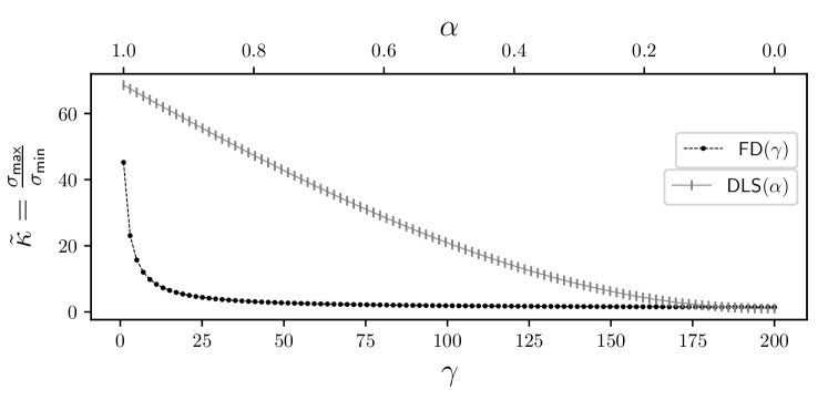
Figure 7: Ill conditioning $\kappa$ for the DLS and FD method. Each data point is the median of $1000$ randomly evaluated joint configurations

It can be seen that FD converges much faster to beneficial condition numbers over its own parameter space than DLS. In fact, most of the decoupling effect from experiment Fig. 6 is already available for low values of $\gamma$.

4.3 Behavior in singularities

Before reporting on this experiment, we briefly recapitulate desired and expected behavior in singularities. In singular configurations, the manipulator Jacobian $\bm{J}$ becomes rank-deficient. This is an unfortunate joint configurations for all considered approaches. As a consequence, the manipulator is not able to achieve instantaneous motion in all directions Murray1994 (21). Two issues arise from this constellation: First, Jacobian transpose-based methods tend to loose manipulability. We measure this effect with $\sigma_{\text{min}}$ of the mapping matrix, which is one of various established measures Murray1994 (21). Second, for Jacobian inverse-based methods, infinite joint velocity occurs. We measure this effect with $\sigma_{\text{max}}$ as an indicator of how much the mapping matrix scales $\bm{f}^{c}$ in sensitive dimensions to joint space. The goal of the experiment is to investigate how well each approach behaves in singular configurations concerning both measures. As a reference, Fig. 8 shows both the Jacobian inverse and the Jacobian transpose for a pass through four singular configurations, the first two being close together.

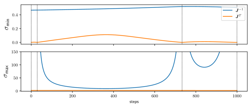
Figure 8: The two baselines $\bm{J}^{T}$ and $\bm{J}^{-1}$ while passing through four singular configurations, illustrated with dashed, vertical lines.

The curves show the expected and well-known effect: The Jacobian inverse maintains high manipulability at the cost of an exploding $\sigma_{\text{max}}$, while the Jacobian transpose stays stable throughout the pass but cannot avoid $\sigma_{\text{min}}$ dropping to zero in singularities.

Fig. 9 and Fig. 10 finally show the behavior of forward dynamics with a set of different $\gamma$. The curves show how FD approaches the Jacobian inverse while maintaining $\sigma_{\text{max}}$ in stable ranges. We added the DLS method, albeit with only one $\alpha$, for comparison. Both FD and DLS have very similar characteristics and show a good trade-off between both corner cases (JI, and JT). Note how the curves for FD become more pronounced towards the Jacobian inverse for increasing $\gamma$.

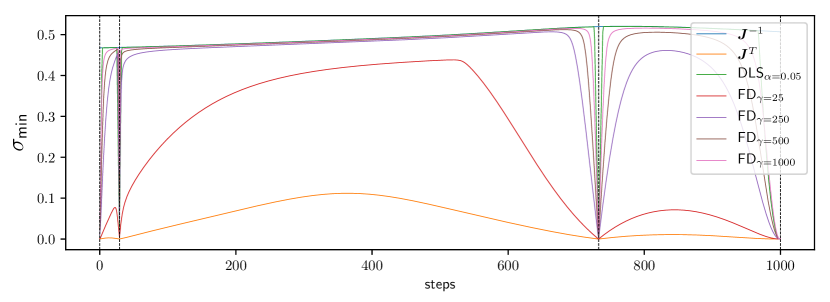
Figure 9: Investigation of $\sigma_{\text{min}}$ of various mapping matrices through four singular configurations.

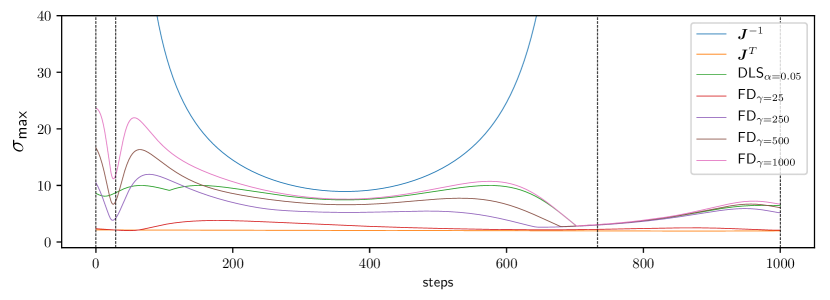
Figure 10: Investigation of $\sigma_{\text{max}}$ of various mapping matrices through four singular configurations.

4.4 Empirical analysis of stability and manipulability

In this experiment, we wanted to analyze FD in comparison to DLS on a broader scale. The goal is an empirical analysis of varying $\alpha$ (DLS) and $\gamma$ (FD) over bigger ranges, and evaluate how they perform in the corner cases in comparison to the Jacobian inverse and transpose. Instead of focusing a few trajectories, we sampled a massive amount of singular constellations. Note that in contrast to the workspace sampling for experiment 4.1, which contained singular configurations by chance, in this investigation we exclusively used singular configurations. Through exclusively focusing regions of low performance (singularities) throughout the whole workspace, the results become a feasible measure of global performance for each method.

To find a big amount of singular configurations, we first sampled equally distributed, random joint states as start configurations. We then used Particle Swarm Optimization (PSO) Miranda2018PySwarms (22), which implements an adapted algorithm from the original work of Kennedy1995 (23) as a black-box optimizing strategy to converge to singular configurations from these start states. We used Yoshikawa’s manipulability measure $\sqrt{\text{det}(\bm{J}\bm{J}^{T})}$, which simplifies for non-redundant mechanisms to $\lvert\text{det}(\bm{J})\rvert$ Yoshikawa1985Manipulability (24) as function to minimize, which was faster than using SVD with $\sigma_{\text{min}}$ directly. Alternatively, a more type-based approach of finding singularities is discussed in Zlatanov1998 (25), Bohigas2012Numerical (26).

Having a set of $1000$ singular configurations, we then computed average values for $\sigma_{\text{min}}$ and $\sigma_{\text{max}}$ from the mapping matrices of FD and DLS according to Fig. 5(a) for discrete values of $\alpha$ and $\gamma$ for each of the $1000$ singular configurations. Fig. 11 shows the results for manipulability. Both DLS and FD approach the Jacobian inverses behavior for decreasing $\alpha$ and increasing $\gamma$, respectively. Note how FD approaches qualitatively faster in its own parameter space.

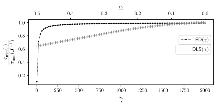
Figure 11: Relative manipulability for the DLS and FD method in comparison to $\bm{J}^{-1}$. Note, that practical applications of the DLS method may require higher damping values of up to $\alpha=1.1$ as reported in Buss2005 (14)

Fig. 12 shows the results for stability.

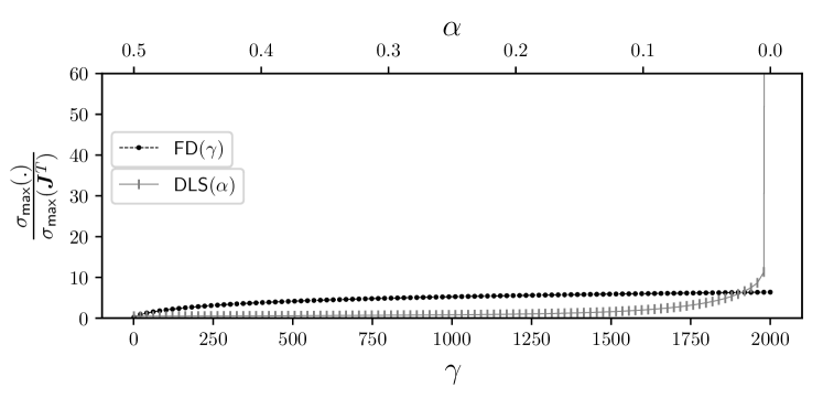
Figure 12: Relative instability for the DLS and FD method in comparison to $\bm{J}^{T}$.

DLS comes closer to the Jacobian transposes stability than FD throughout most of the observed parameter space. However, towards reaching the Jacobian inverses high manipulability, DLS looses stability and asymptotically approaches infinity, while FD in contrast stays bounded. For applications in which DLS would require very low values of $\alpha$ for control performance, FD can be used as a safe alternative, combining and keeping the benefits of both $\bm{J}^{-1}$ and $\bm{J}^{T}$.

4.5 Computational efficiency

Finally, we measured average execution times of the mapping approaches. We implemented the SDLS method according to Buss2005 (14) and included the measurements as additional reference.

To obtain the comparison, we computed $\ddot{\bm{q}}$ as given in Fig. 5(a) with a fictitious, constant $\bm{f}^{c}=\bm{1}$ for $10e5$ times. The joint state $\bm{q}$ was randomly sampled, while being identical across one single evaluation of each method. Fig. 13 shows the boxplots of each method’s execution time with their quartiles. The median is plotted as vertical, orange line. The whiskers for minimal an maximal execution times indicate a high degree of irregularity. We expect narrower ranges for experiments on a hard real-time operating system.

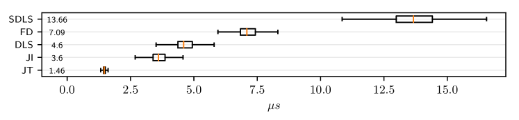
Figure 13: Execution times of computing different mappings of type (a) from Fig. 5 on an Intel^® Core™ i7-4900MQ.

The results show that the forward dynamics method is a little more computationally intense than the DLS method, but approximately half the execution time of the SDLS. Being still in the low $\mu$s range makes forward dynamics in the version from this paper suitable for real-time closed-loop control.

5 Discussion

5.1 Virtual forward models

When deriving our principal mapping for forward dynamics in Eq. (10), we dropped gravity and non-linear terms to support dynamics decoupling of our virtual system. For redundant manipulators, including those terms offers additional interfaces to adjust behavior in the nullspace of the Jacobian transpose. For those cases, switching from the composite rigid body algorithm to propagation methods for solving the forward dynamics might be beneficial. The articulated body algorithm Featherstone1983 (18), e.g. allows an intuitive integration of external loads to each link of the robot separately, which might be used to implement collision avoidance or other optimizations concerning the robots’ posture.

5.2 Control applications

The natural mapping of forward dynamics from Cartesian wrench space to joint accelerations makes it particularly suitable for the implementation of admittance-related controllers on velocity-actuated systems. For those use cases, force-resolved control laws for disturbance rejection can replace the velocity-resolved control laws using DLS. The benefit of using the FD method is its ability to operate extremely close to the ideal $\bm{J}^{-1}$ behavior without significantly sacrificing stability. Successful implementations of forward dynamics-based control on industrial robots can be found e.g. in Scherzinger2019Contact (27) for pure force control and in Scherzinger2017 (9), Heppner2020 (28) for compliance control. An application to motion control with a particular focus on sparsely sampled targets is presented in Scherzinger2019Inverse (10).

6 Conclusion

This paper proposed virtual forward dynamics models for Cartesian robot control. The core of the control loop is a simplified, virtual model that maps Cartesian control signals to joint accelerations. Through increasing the end effector’s mass in comparison to the other links, the virtual system becomes linear in the operational space dynamics and matches the exactness of the Jacobian inverse. Further experiments showed, that this forward model’s decoupling leads to less ill conditioning compared to the DLS method for an empirical investigation of the joint space. When passing through singularities, forward dynamics behaves in general similar to DLS in terms of manipulability and stability. Yet, when operating in singular configurations forward dynamics models substantially differ from DLS in that they produce bounded control signals, even when forced to approach the Jacobian inverse in terms of manipulability. These virtual forward models are particularly suitable for implementing admittance controllers in industrial settings on velocity-actuated robots. Their computation time in the low $\mu$s range makes them suitable for real-time control.

References

- (1) Daniel E Whitney “Force feedback control of manipulator fine motions”, 1977
- (2) Marc H Raibert and John J Craig “Hybrid position/force control of manipulators” In Journal of Dynamic Systems, Measurement, and Control 102.127, 1981, pp. 126–133
- (3) O. Khatib “A unified approach for motion and force control of robot manipulators: The operational space formulation” In IEEE Journal on Robotics and Automation 3.1, 1987, pp. 43–53 DOI: 10.1109/JRA.1987.1087068
- (4) S. Chiaverini and L. Sciavicco “The parallel approach to force/position control of robotic manipulators” In IEEE Transactions on Robotics and Automation 9.4, 1993, pp. 361–373
- (5) N. Hogan “Impedance control - An approach to manipulation. I - Theory. II - Implementation. III - Applications” In ASME Transactions Journal of Dynamic Systems and Measurement Control B 107, 1985, pp. 1–24
- (6) Luigi Villani and Joris De Schutter “Force control” In Springer handbook of robotics Springer, 2008, pp. 161–185
- (7) Roy Featherstone “Rigid body dynamics algorithms” Springer, 2008
- (8) C.. Wampler “Manipulator Inverse Kinematic Solutions Based on Vector Formulations and Damped Least-Squares Methods” In IEEE Transactions on Systems, Man, and Cybernetics 16.1, 1986, pp. 93–101 DOI: 10.1109/TSMC.1986.289285
- (9) S. Scherzinger, A. Roennau and R. Dillmann “Forward Dynamics Compliance Control (FDCC): A new approach to cartesian compliance for robotic manipulators” In IEEE/RSJ International Conference on Intelligent Robots and Systems (IROS), 2017, pp. 4568–4575 DOI: 10.1109/IROS.2017.8206325
- (10) S. Scherzinger, A. Roennau and R. Dillmann “Inverse Kinematics with Forward Dynamics Solvers for Sampled Motion Tracking” In 2019 19th International Conference on Advanced Robotics (ICAR), 2019, pp. 681–687 DOI: 10.1109/ICAR46387.2019.8981554
- (11) William A Wolovich and H Elliott “A computational technique for inverse kinematics” In The 23rd IEEE Conference on Decision and Control, 1984, pp. 1359–1363 URL: http://ieeexplore.ieee.org/abstract/document/4048118/
- (12) Yoshihiko Nakamura and Hideo Hanafusa “Inverse kinematic solutions with singularity robustness for robot manipulator control” In ASME, Transactions, Journal of Dynamic Systems, Measurement, and Control 108, 1986, pp. 163–171
- (13) Samuel R Buss “Introduction to inverse kinematics with jacobian transpose, pseudoinverse and damped least squares methods” In IEEE Journal of Robotics and Automation 17.1-19, 2004, pp. 16
- (14) Samuel R Buss and Jin-Su Kim “Selectively damped least squares for inverse kinematics” In Journal of Graphics tools 10.3 Taylor & Francis, 2005, pp. 37–49 URL: https://www.tandfonline.com/doi/abs/10.1080/2151237X.2005.10129202
- (15) Marc G Carmichael, Dikai Liu and Kenneth J Waldron “A framework for singularity-robust manipulator control during physical human-robot interaction” In The International Journal of Robotics Research 36.57, 2017, pp. 861–876 DOI: 10.1177/0278364917698748
- (16) S. McMillan and D.. Orin “Forward dynamics of multilegged vehicles using the composite rigid body method” In Proceedings. 1998 IEEE International Conference on Robotics and Automation (Cat. No.98CH36146) 1, 1998, pp. 464–470 vol.1 URL: https://ieeexplore.ieee.org/abstract/document/677017
- (17) Roy Featherstone “Efficient Factorization of the Joint-Space Inertia Matrix for Branched Kinematic Trees” In The International Journal of Robotics Research 24.6, 2005, pp. 487–500 DOI: 10.1177/0278364905054928
- (18) R. Featherstone “The Calculation of Robot Dynamics Using Articulated-Body Inertias” In The International Journal of Robotics Research 2.1, 1983, pp. 13–30 DOI: 10.1177/027836498300200102
- (19) Morgan Quigley et al. “ROS: an open-source Robot Operating System” In ICRA workshop on open source software 3.3.2, 2009, pp. 5 URL: http://www.willowgarage.com/papers/ros-open-source-robot-operating-system
- (20) Roy Featherstone “An Empirical Study of the Joint Space Inertia Matrix” In The International Journal of Robotics Research 23.9, 2004, pp. 859–871 DOI: 10.1177/0278364904044869
- (21) Richard M Murray, Zexiang Li, S Shankar Sastry and S Shankara Sastry “A mathematical introduction to robotic manipulation” CRC press, 1994
- (22) Lester Miranda “PySwarms: a research toolkit for particle swarm optimization in Python” In Journal of Open Source Software 3.21, 2018, pp. 433
- (23) J. Kennedy and R. Eberhart “Particle swarm optimization” In Proceedings of ICNN’95 - International Conference on Neural Networks 4, 1995, pp. 1942–1948 vol.4 URL: https://ieeexplore.ieee.org/abstract/document/488968
- (24) Tsuneo Yoshikawa “Manipulability of Robotic Mechanisms” In The International Journal of Robotics Research 4.2, 1985, pp. 3–9 DOI: 10.1177/027836498500400201
- (25) D. Zlatanov, R.G. Fenton and B. Benhabib “Identification and classification of the singular configurations of mechanisms” In Mechanism and Machine Theory 33.6, 1998, pp. 743–760 DOI: https://doi.org/10.1016/S0094-114X(97)00053-0
- (26) O. Bohigas et al. “Numerical computation of manipulator singularities” In 2012 IEEE International Conference on Robotics and Automation, 2012, pp. 1351–1358 URL: https://ieeexplore.ieee.org/document/6225083
- (27) S. Scherzinger, A. Roennau and R. Dillmann “Contact Skill Imitation Learning for Robot-Independent Assembly Programming” In 2019 IEEE/RSJ International Conference on Intelligent Robots and Systems (IROS), 2019, pp. 4309–4316 DOI: 10.1109/IROS40897.2019.8967523
- (28) Georg Heppner et al. “FLA2IR—FLexible Automotive Assembly with Industrial Co-workers” In Bringing Innovative Robotic Technologies from Research Labs to Industrial End-users: The Experience of the European Robotics Challenges Cham: Springer International Publishing, 2020, pp. 97–126 DOI: 10.1007/978-3-030-34507-5_5