Thermal effects in non-Fermi liquid superconductivity

Abstract

We revisit the interplay between superconductivity and quantum criticality when thermal effects from virtual static bosons are included. These contributions, which arise from an effective theory compactified on the thermal circle, strongly affect field-theoretic predictions even at small temperatures. We argue that they are ubiquitous in a wide variety of models of non-Fermi liquid behavior, and generically produce a parametric suppression of superconducting instabilities. We apply these ideas to non-Fermi liquids in $d=2$ space dimensions, obtained by coupling a Fermi surface to a Landau-damped soft boson. Extending previous methods developed for $d=3-\epsilon$ dimensions, we determine the dynamics and phase diagram. It features a naked quantum critical point, separated by a continuous infinite order transition from a superconducting phase with strong non-Fermi liquid corrections. We also highlight the relevance of these effects for (numerical) experiments on non-Fermi liquids.

I Introduction

Quantum criticality is thought to play a central role in the dynamics and superconductivity of strongly correlated electronic systems Sachdev ; RevModPhys.79.1015 ; keimer4673high ; SHE2010S911 ; Zaanen2004 ; Eschrig2006 ; PhysRevLett.124.076801 ; Shibauchi2014 ; Mathur1998 ; Putzke2014 ; Dahm2009 ; LeTacon2011 ; Park2006 ; Chatterjee9346 ; Ramshaw317 . The proliferation of emergent gapless modes interacting with the electrons leads to many exciting phenomena, broadly characterized as “non-Fermi liquid” (NFL) behavior . Over the last decades, there has been fundamental progress, both experimental and theoretical, on the physics of strongly correlated materials. But the mechanisms behind high $T_{c}$ superconductivity and its connection with quantum criticality are not fully understood yet.

The interplay between quantum effects and superconductivity is in general quite nontrivial due to two competing tendencies of soft bosons: i) the destruction of coherent quasiparticles; ii) the enhancement of the superconducting pairing channel. Theoretically, it is possible to envision a rich landscape of possibilities ranging from an NFL state completely hidden under a superconducting dome Polchinski1994 ; Altshuler1994 ; Metlitski , to having a naked quantum critical point (QCP) Raghu:2015sna ; Wang:2016hir . However, tractable field theory models usually require some expansion parameter (like Migdal’s approximation migdal1958interaction ; abrikosov2012methods ), and this has been an obstacle for comparing with real materials or with numerical experiments, which often lack such a parameter.

The goal of this work is to further develop the field theory framework for analyzing the interplay between quantum criticality and superconductivity. This continues previous lines of research Raghu:2015sna ; Wang:2016hir ; Wang:2017teb ; Damia:2019bdx ; Damia:2020yiu . We incorporate both quantum and finite temperature effects, relevant for comparison with experiments. Previous studies at zero temperature $T=0$ in two spatial dimensions found that superconductivity is enhanced in NFLs when soft bosons come from order parameters, and that a stable naked QCP does not exist; on the other hand, superconductivity was found to be parametrically decreased or destroyed in the case of emergent $U(1)$ gauge fields Metlitski ; lee2007amperean ; wang2014pairing .

At finite temperature we uncover a much richer dynamics that builds on two key points. First, we identify a parameter ‘$N$’ that measures the ratio between quantum corrections to the self-energy and corrections to the superconducting gap. As discussed in Sec. II, many different NFLs have $N>1$, while $N=1$ in more standard Fermi liquids. Secondly, we demonstrate that the exchange of virtual bosons of zero Matsubara frequency (static modes) gives new contributions that tend to decrease the superconducting instability and can even lead to a naked QCP with critical pairing interactions.

These virtual static contributions are a bit similar to impurity effects and have been traditionally neglected on the basis of Anderson’s theorem anderson1959theory ; millis1988inelastic ; PhysRevB.78.220507 ; 2016PhRvL.117o7001W . However, we argue that they do not cancel precisely when $N>1$. As a result, the dynamics is qualitatively different depending on $N=1$ versus $N>1$. Furthermore, $N$ does not need to be large in order to observe the non-cancellation of thermal effects from static modes. Even in NFLs where the emergent bosons are order parameters, we then find that superconductivity can be enhanced or diminished depending on the parameter $N$. The notorious differences between $N=1$ and $N>1$ dynamics provide nontrivial signatures that would be very interesting to target in future numerical experiments.

The main general lesson from our analysis will be that it is crucial to take into account effects from virtual zero frequency bosons at finite temperature. These static modes will be seen to play a major role in the interplay between quantum criticality and superconductivity in correlated electronic systems with $N>1$. Intuitively, they arise from an effective theory in one less dimension, obtained by compactifying on the thermal circle. For this reason, they are not governed by the scaling laws of the $T=0$ theory. We will argue that the resulting phase diagram at finite $T$ is very different from that based on naive $T=0$ expectations. An explicit analysis of the equations governing the fermion self-energy and superconducting gap require some specific information about the model (dispersion relations, Fermi surface geometry, etc.). We will do this for the well-known QCP with dynamical scaling $\omega^{2/3}\sim p$ that obtains from coupling a Fermi surface to an overdamped boson. But we would like to stress here that the basic result on the role of the static modes and $N>1$ is more general and should be analyzed in other models as well.

This paper is organized as follows. First in Sec. II we present a more or less general discussion of thermal effects, the contribution of virtual static bosonic modes and the role of the parameter $N$. While concrete calculations require more explicit model-dependent assumptions (the subject of the following sections), the goal here is to argue for the generality of such effects in NFLs. In Sec. III we briefly review the more specific theory that we will study, obtained by coupling a Fermi surface to Landau damped bosons. Our main results are in Sec. IV, where we study the superconducting instability at linearized level and its critical temperature, obtaining the phase diagram and exhibiting the key effects from $N$ and the thermal static modes. The normal state is found to be stable for $N>N_{cr}\sim 8$; a superconducting instability develops via an infinite-order transition as $N\to N_{cr}$, and the ground state is a superconductor for $N<N_{cr}$. This phase exhibits strong NFL and thermal effects, most notably a parametric suppression of the critical temperature compared to the physical gap. In Sec. V we explore the gap equation at nonlinear level, looking for solutions that may have been missed in the linearized treatment. We indeed find a different type of solution that is predominantly sourced by the first few Matsubara modes of the gap. However, we argue that the above thermal effects imply that this solution is never energetically preferred. Therefore our results for the dynamics and phase diagram appear consistent also at the nonlinear level. We also briefly compare this situation with the related (but eventually quite different) scenario of the “first Matsubara law” analyzed in recent works 2016PhRvL.117o7001W ; 2019PhRvB..99n4512W ; 2019arXiv191201797C ; Abanov_2020 ; Wu_2020 . Finally, we summarize the main conclusions and future directions in Sec. VI. Two appendices contain somewhat more technical results that are used in the main text.

II Thermal effects on fermion self-energy and gap

Non-Fermi liquid behavior arises generically from interactions between a Fermi surface and soft bosons. The same interaction that produces interesting quantum physics simultaneously leads to strong thermal corrections. Our goal in this section is to present a discussion of finite temperature effects at a general level, making manifest that they will be ubiquitous for a broad class of models. In the following sections we will perform a detailed analysis for a class of NFLs with Landau damped bosons.

Consider a coupling of the Yukawa form $H_{int}=g\phi\psi^{\dagger}\psi$, and denote the boson propagator by $D(q,\Omega)$, with $q$ the momentum and $\Omega$ the frequency of the boson. At one and higher loops, virtual bosons lead to a fermion self-energy $\Sigma$ and, possibly, to the formation of a superconducting gap $\Delta$. Generically there will also be vertex corrections, but we will neglect them here. In order to exhibit the thermal corrections in their simplest form, it is sufficient to keep only the linear effects from the gap. This is also the physically relevant regime for studying the putative superconducting transition; in Sec. V we will analyze nonlinear effects from the gap.

Given these simplifications, the fermion dynamics is determined by two self-consistent Schwinger-Dyson equations. The first fixes the self-energy,

$$i\Sigma(p,\omega_{n} )=-g^{2}T\sum_{m}\int\frac{d^{d}q}{(2\pi)^{d}}D(p-q,\omega_{n}-\omega_{m})$$

$$\times\frac{1}{i\omega_{m}+i\Sigma(q,\omega_{m})-\varepsilon_{q}}$$ (II.1)

where $\varepsilon_{q}$ is the classical fermion dispersion relation, $n,m$ are discrete Matsubara indices and $d$ is the number of spatial dimensions. The second self-consistent equation, also known as the Eliashberg equation, determines the gap

$$\tilde{\Delta}(p,\omega_{n}) =\frac{g^{2}}{N}T\sum_{m}\int\frac{d^{d}q}{(2\pi)^{d}}D(p-q,\omega_{n}-\omega_{m})$$

$$\times\frac{\tilde{\Delta}(q,\omega_{m})}{\left(\omega_{m}+\Sigma(q,\omega_{m})\right)^{2}+\varepsilon_{q}^{2}}\,.$$ (II.2)

Here $\tilde{\Delta}$ is the pairing vertex, that appears directly in the Hamiltonian, $H\supset\tilde{\Delta}\psi_{p}\psi_{-p}+c.c.$; it is related to the physical gap by

$$\tilde{\Delta}(p,\omega_{n})=\left(1+\frac{\Sigma(p,\omega_{n})}{\omega_{n}}\right)\Delta(p,\omega_{n})\,.$$ (II.3)

We have introduced a parameter $N>1$ that distinguishes the strength of corrections to the self-energy and the gap. Let us explain our reasons and motivations behind this. In the simplest cases of BCS or phonon superconductivity, $N=1$, but $N>1$ is motivated by non-Fermi liquid physics. Indeed, one of the original examples for this is in color superconductivity, where $N=3$ from the $SU(3)$ gauge interaction of chromodynamics Son:1998uk . Strongly correlated electronic systems can also have matrix-type order parameters that give $N>1$, as in antiferromagnetic type materials 2012RvMP…84.1383S . $N$ can also be related to unconventional superconductivity with nonzero angular momentum. More recently, new materials have been constructed that display approximate global symmetries that translate to $N>1$. This includes the valley symmetry in graphene and could also be relevant for the exciting discoveries in twisted bilayer graphene 2018Natur.556…43C ; cao2018magic ; cao2020strange ; po2018origin ; wang2020topological ; baskaran2018theory ; roy2019unconventional ; isobe2018unconventional ; dodaro2018phases ; you2019superconductivity . Another motivation is to have QFT predictions to compare with future numerical experiments on the lattice. This is now especially relevant given recent progress in Monte Carlo methods Schattner2016 ; 2017PNAS..114.4905L ; Berg2019 ; liu2019itinerant ; klein2020normal ; Xu:2020tvb . One of our main results will be that $N>1$ leads to thermal effects that are qualitatively different from $N=1$, and this provides nontrivial signatures to look for numerically.

In the euclidean formalism, finite temperature contributions are represented by the Matsubara sums in (II) and (II), with $\omega_{n}=\pi T(n+1/2)$. Small temperature means $n$ large, and in this limit one expects to recover the $T=0$ results plus corrections. However, the terms with $m=n$ in the sum can lead to large departures from this. They come from exchange of static bosons with $\Omega_{n}=0$. Such contributions can be analyzed with an effective theory in one less space-time dimension, obtained by compactifying on the thermal circle. As a result, static effects do not need to respect the scaling laws of the $T=0$ theory, and indeed can lead to large violations of these. Our goal is to determine how these thermal contributions affect superconductivity in non-Fermi liquids.

Virtual static bosons resemble impurities, and have often been neglected in previous works on the basis of Anderson’s theorem anderson1959theory ; millis1988inelastic ; PhysRevB.78.220507 ; 2016PhRvL.117o7001W . We will review that the reason for this is that they can be rescaled away when $N=1$. Crucially, however, this cancellation will be seen to fail for $N>1$, see Sec. IV.2 below. This is why thermal physics will be very different. Non-cancellation of thermal static effects will modify the behavior of the gap $\Delta$ and the superconducting transition $T_{c}$, as well as generically producing a parametric difference $T_{c}\ll\Delta$. This is potentially relevant for unconventional superconductors with such a hierarchy of scales 2012JPSJ…81a1006Y ; 2016NatCo…712843K .

The way to study and solve (II) and (II) is somewhat model-dependent. In this work we will focus on a spherical Fermi surface and the well-known quantum critical scaling for the fermion $\Sigma(\omega)\sim\omega^{2/3}$. The methods we develop may also be applied to other dynamical exponents and/or geometries, and we hope to address these in future work. Despite this model dependence, let us make some remarks that should apply more generally to non-Fermi liquids.

The first is that the non-cancellation of thermal effects is expected when $N\neq 1$. This does not require $N\gg 1$, but works for any $N>1$. From this point of view, $N=1$ may be a choice that is non-generic for the dynamics of NFLs and their interplay with superconductivity. The second point to stress is that once thermal effects from static boson exchange contribute, they are expected to tend to diminish the superconducting gap, and correspondingly increase the NFL region above the superconducting dome. The reason is that, as we discussed before, we can think of them as arising from an effective theory in one less dimension, and decreasing the dimensionality tends to disorder the ground state. We will see explicitly how this comes about. The parameter $N$ could then be relevant for explaining why certain NFLs have an enhanced superconducting temperature $T_{c}$, while in others $T_{c}$ is decreased. It would be interesting to revisit models of strange metals in light of the results in this work.

Finally, let us stress that we are considering a different situation from that of a series of recent works on the interplay between superconductivity and quantum criticality 2016PhRvL.117o7001W ; 2019PhRvB..99n4512W ; 2019arXiv191201797C ; Abanov_2020 ; Wu_2020 . Those references analyze equations similar to (II) and (II) but removing $m=n$ terms. Their focus is on $N=1$ where $m=n$ terms can be rescaled away, and the parameter $N$ in these works is a way of dialing the relative strength of quantum critical and superconducting contributions. In contrast, in our work $N$ is physical as we motivated before, and thermal effects from virtual static bosons will turn out to play a fundamental role. This is the reason why our results are different from those works; a more detailed comparison will be presented in Sec. V.5.

III Model and dynamics at zero temperature

The rest of the paper is devoted to analyzing the interplay between quantum criticality and superconductivity at finite temperature in a concrete NFL model. We will demonstrate the failure of Anderson’s cancellation of static effects for $N>1$, and we will obtain the phase diagram that is qualitatively changed due to thermal effects. In this section we review the model and study its dynamics at $T=0$. We first discuss the two-dimensional quantum critical point of Damia:2019bdx , based on a Fermi surface interacting with soft bosons via a Yukawa coupling. In the second step we add BCS 4-Fermi couplings and use the renormalization group and Schwinger-Dyson equations to study their effects on the fixed point.

III.1 Non-Fermi liquid fixed point

We consider a model of non-Fermi liquids where a Fermi surface (taken to be spherical for simplicity) of fermions $\psi$ is coupled to a Landau-damped massless scalar $\phi$ with $z_{b}=3$ dynamical exponent. Following previous works Fitzpatrickone ; Mahajan2013 ; FKKRtwo ; Torroba:2014gqa , $\psi^{i}$ is promoted to an $N$-component field, while $\phi^{i}_{j}$ is an $N\times N$ matrix. This parameter $N>1$ will lead to the non-cancellation of thermal static effects.

We start from the following low energy effective action that respects the $SU(N)$ symmetry:

$$S=S_{f}+S_{b}+S_{Y}$$ (III.1)

with

$$S_{f} = -\int_{\omega,p}\psi^{\dagger}_{i}(i\omega-\varepsilon_{p})\psi^{i}$$

$$S_{b} = \frac{1}{2}\int_{\Omega,q}\phi_{i}^{j}\left(q^{2}+M_{D}^{2}\frac{|\Omega|}{q}\right)\phi_{j}^{i}$$ (III.2)

$$S_{Y} = \frac{g}{\sqrt{N}}\int_{\omega,p}\int_{\Omega,q}\phi_{j}^{i}(\Omega,q)\psi_{i}^{\dagger}(\omega,p)\psi^{j}(\omega-\Omega,p-q)\,.$$

Here $M_{D}$ is the Landau damping mass scale, and we take it as the UV cutoff in our effective description. The bare mass for the boson is tuned to zero to approach the quantum critical point. Given this tuning, the Yukawa interaction with strength $g$ is the most relevant one consistent with the $SU(N)$ symmetry. Except for the marginal BCS scattering that we will introduce shortly, other interactions turn out to be irrelevant at the fixed point.

The spherical dispersion relation

$$\varepsilon_{p}=\frac{p^{2}}{2m}-\mu_{F}\,,$$ (III.3)

gives a Fermi surface of radius $k_{F}=\sqrt{2m\mu_{F}}$. Since we are interested in the low energy/momenta dynamics, it will be sufficient to linearize

$$\varepsilon_{p}\approx vp_{\perp}\;,\;\vec{p}\equiv\hat{n}(k_{F}+p_{\perp})$$ (III.4)

with $\hat{n}$ a unit vector on the Fermi surface. This is the spherical RG of Shankar .

It was recently shown in Damia:2019bdx that, in the large $N$ limit, (III.1) leads to a controlled quantum critical point with non-Fermi liquid behavior. Below the dynamical scale

$$\Lambda=\frac{g^{6}}{(2\pi v\sqrt{3})^{3}M_{D}^{2}}\,,$$ (III.5)

the theory flows to a fixed point with fermion self-energy

$${\Sigma_{\text{NFL}}}(\omega)=\Lambda^{1/3}{\rm sgn}(\omega)|\omega|^{2/3}\,,$$ (III.6)

that gives a $z_{f}=3/2$ dynamical exponent. All other effects at the fixed point (including corrections to the boson 2-point function) are suppressed by $1/N$. We stress that we start with a Landau-damped $z=3$ boson, and that’s why we take $M_{D}$ as the UV cutoff; this is required in order to avoid the large $N$ problems found in Lee2009 . By itself, the low energy dynamics also generates a Landau-damping contribution, but it is suppressed by $1/N$.

Our goal in what follows is to study the competition between non-Fermi liquid behavior and the superconducting instability in this setup, first at zero temperature and then taking into account thermal effects.

III.2 Incorporating the BCS interaction

Let us now include the 4-Fermi interaction in the BCS channel. We briefly discuss both the renormalization group approach, following Shankar ; Polchinski ; Son:1998uk ; Metlitski ; Raghu:2015sna , and the Eliashberg method. Boson exchange in (III.1) leads to a non-local 4-Fermi interaction. The idea of the RG, first explained in Son:1998uk , is that part of this non-local term becomes local when integrating over momentum or frequency shells, and hence contributes to the BCS beta function. This approach was generalized in Raghu:2015sna to incorporate the fermion anomalous dimensions, and that is the version we will use here.

It is convenient to normalize the BCS coupling as follows,

$$H_{\text{BCS}}=-\frac{v}{4k_{F}N}\lambda\,(\psi^{\dagger}\psi\psi^{\dagger}\psi)$$ (III.7)

where the fermion’s momenta (not shown here) are on the BCS channel Shankar ; Polchinski . The prefactor $v/(4k_{F})$ is chosen to simplify formulas, and the $1/N$ reflects the non-planar character of the BCS scattering. There are three contributions to the RG beta function of the BCS coupling $\lambda$ Raghu:2015sna . Let us analyze them in turn.

First, tree-level boson exchange contributes a source term proportional to $g^{2}$ that accounts for the boson-mediated interaction that becomes local Son:1998uk . Integrating out the boson generates an effective non-local interaction

$$S_{int}=-\frac{g^{2}}{2N}\int_{q,p,p^{\prime}}\,D(q)\,\psi_{i}^{\dagger}(p)\psi^{j}(p-q)\,\psi_{j}^{\dagger}(p^{\prime})\psi^{i}(p^{\prime}+q)\,.$$ (III.8)

This interaction is attractive, so it will be sufficient to consider $s$-wave pairing. Using this and the $z_{b}=3$ scaling of the boson leads to a frequency-dependent pairing

$$\frac{g^{2}}{2N}\,\int\frac{dq_{\parallel}}{2\pi}\,D(\Omega,q_{\parallel})=\frac{1}{N}\,\frac{g^{2}}{3\sqrt{3}}\,\frac{1}{(M_{D}^{2}|\Omega|)^{1/3}}$$ (III.9)

where $q_{\parallel}$ here is the bosonic momentum orthogonal to the local $\vec{k}_{F}$. The tree-level contribution to the beta function of the BCS coupling is obtained by deriving (III.9) with respect to $\Omega$.

The next contribution comes about because in a non-Fermi liquid the fermions acquire a positive anomalous dimension, and this makes the BCS coupling irrelevant Raghu:2015sna . At large $N$, the fermion anomalous dimension is $\gamma=1/6$ (defined as changing the classical frequency term by $\omega\to\omega^{1-2\gamma}$). By itself, this is a large effect at the fixed point, giving an irrelevant scaling dimension $[\lambda]=-1/3$. If it were for this contribution alone, we would have $\lambda\to 0$. The last contribution comes from the one loop fermion bubble Shankar , and this is the standard contribution in Fermi liquids.

The resulting beta function at the QCP evaluates to

$$\frac{d\lambda}{d\log\mu}=-\frac{8\pi}{9}+\frac{\lambda}{3}-\frac{\lambda^{2}}{4\pi N}\,.$$ (III.10)

This encodes mathematically the competition between non-Fermi liquid and pairing effects in the beta function: the tree-level exchange and one loop fermion bubble push to make $\lambda$ relevant, while the NFL anomalous dimension tries to make the BCS coupling irrelevant.

A general consequence of beta functions like (III.10) is that they support UV and IR fixed points and give rise to Berezinskii-Kosterlitz-Thouless (BKT) scaling when the fixed points annihilate Kaplan:2009kr . In our case, the fixed points are at

$$\lambda_{\pm}=\frac{2\pi}{3}N\left(1\pm\sqrt{1-8/N}\right)\,,$$ (III.11)

valid for $N>8$. From the slope of the beta function, $\lambda_{-}$ is attractive while $\lambda_{+}$ is repulsive. The resulting RG flow is illustrated in Fig. 1.

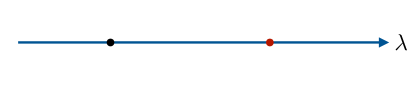
Figure 1: Schematic RG flow of the BCS coupling between UV and IR fixed points.

The stable fixed point at

$$\lambda^{*}=\frac{2\pi}{3}N\left(1-\sqrt{1-8/N}\right)\approx\frac{8\pi}{3}\;\;(\text{for}\;N\gg 1)$$ (III.12)

describes a quantum critical point for the BCS coupling. This was one of the main findings of Raghu:2015sna , a metallic state with critical BCS interactions. The same mechanism discovered in that work, which used an epsilon expansion around $d=3$, also applies here in $d=2$ by virtue of the large $N$ limit. While this is outside the scope of this paper, it would be interesting to understand the phenomenological implications of critical pairing interactions in the physical dimension $d=2$.

Ref. Raghu:2015sna also identified the transition between NFL and superconducting states as an infinite order BKT transition driven by fixed point annihilation. We see the same applies here: as $N\to 8$, the UV and IR fixed points merge and for $N<8$ they go off into the complex plane. In the absence of a stable fixed point, the RG flow of Fig.1 then proceeds to the $\lambda\to\infty$ region; this growth in the pairing attraction signals a superconducting instability, and we will soon analyze this from the point of view of the gap equation. We will see that the value $N_{cr}=8$ receives small corrections from non-local effects that are not captured by the RG. Furthermore such values may be outside the regime of validity of the large $N$ approximation that we have used. It seems plausible that the transition between the normal and superconducting states in the full theory will still occur via BKT scaling, but it would be interesting to analyze the leading $1/N$ corrections and their effect on the fixed-point annihilation picture.

III.3 Eliashberg equation and BKT transition

An alternative approach is to allow for a superconducting gap and derive a self-consistent equation that it should obey. The pairing vertex appears in the Hamiltonian as $H\supset\tilde{\Delta}\psi_{p}\psi_{-p}+c.c.$, and is related to the physical gap $\Delta$ via (II.3) above. A very useful simplification near QCPs like the one we are considering is that both the self-energy and the gap depend predominantly on frequency; this restricts integral and differential equations to just one variable. The self-consistent Schwinger-Dyson equation at $T=0$ is

$$\tilde{\Delta}(p)=\frac{g^{2}}{N}\,\int\frac{d^{3}q}{(2\pi)^{3}}\,\frac{D(p-q)\,\tilde{\Delta}(q)}{|q_{0}+\Sigma(q_{0})|^{2}+|\tilde{\Delta}(q)|^{2}+\varepsilon_{q}^{2}}\,.$$ (III.13)

If the system superconducts, the frequency dependence will stabilize below the physical gap scale, defined as

$$\Delta_{0}\equiv\Delta(\omega=\Delta_{0})\,.$$ (III.14)

As is standard with gap equations, we will approximate this by linearizing the integrand in (III.13), while restricting the frequency integral to $|\omega|>\Delta_{0}$. This value $\Delta_{0}$ will have to be determined self-consistently.

As in (III.9), the $z_{b}=3$ scaling implies that the $q_{\parallel}$ integral affects only the boson propagator, while $q_{\perp}$ appears only in the fermion propagator. Performing the integrals obtains

$$\tilde{\Delta}(\omega)=\frac{\Lambda^{1/3}}{3N}\,\int_{|\omega^{\prime}|>\Delta_{0}}d\omega^{\prime}\frac{1}{|\omega-\omega^{\prime}|^{1/3}}\frac{\tilde{\Delta}(\omega^{\prime})}{|\omega^{\prime}+\Sigma(\omega^{\prime})|}\,.$$ (III.15)

This is the familiar Eliashberg equation for the gap, here evaluated with retardation effects from the soft $z_{b}=3$ boson. We focus on a gap that is even in frequency. Then the linearized gap equation rewrites to

$$\tilde{\Delta}(\omega)=\frac{1}{2N}\int_{\Delta_{0}}^{\Lambda_{0}}d\omega^{\prime}\,u(\omega,\omega^{\prime})\frac{\tilde{\Delta}(\omega^{\prime})}{A(\omega^{\prime})}$$ (III.16)

with $\Lambda_{0}$ a UV frequency cutoff, $A(\omega)=\omega+\Lambda^{1/3}|\omega|^{2/3}$ and

$$u(\omega,\omega^{\prime})=\frac{2\Lambda^{1/3}}{3}\left(\frac{1}{|\omega-\omega^{\prime}|^{1/3}}+\frac{1}{|\omega+\omega^{\prime}|^{1/3}}\right)\,.$$ (III.17)

As shown in Wang:2016hir in the analog problem in $d=3-\epsilon$ dimensions, the RG result is recovered in a local approximation where frequency mixing in (III.15) is small. We will find that this is also a very good approximation in $d=2$, up to small corrections that will be determined via numerics and will be incorporated below in Sec. IV.

By means of a local approximation $u(\omega,\omega^{\prime})\approx 2u(\omega)$ ($u(\omega,\omega^{\prime})\approx 2u(\omega^{\prime})$) for $\omega>\omega^{\prime}$ ($\omega<\omega^{\prime}$), (III.16) can be mapped to a differential equation of the form

$$\frac{d}{d\omega}\left(\frac{\tilde{\Delta}^{\prime}(\omega)}{u^{\prime}(\omega)}\right)=\frac{\tilde{\Delta}(\omega)}{NA(\omega)}$$ (III.18)

together with the UV and IR boundary conditions inherited from the integral equation,

$$\frac{d}{d\omega}\left(\frac{\tilde{\Delta}(\omega)}{u(\omega)}\right)\Big{|}_{\omega=\Lambda_{0}}=0\;,\;\tilde{\Delta}^{\prime}(\omega)\Big{|}_{\omega=\Delta_{0}}=0\,.$$ (III.19)

The change of variables

$$\lambda(\omega)=\frac{8\pi}{3}\,\frac{u^{\prime}(\omega)}{u(\omega)}\,\frac{\tilde{\Delta}(\omega)}{\tilde{\Delta}^{\prime}(\omega)}$$ (III.20)

transforms the differential problem into the RG beta function, thus establishing their equivalence.

Let us now analyze the transition between quantum criticality and superconductivity using the gap equation. Following Wang:2016hir (similar calculations have also appeared more recently in 2019arXiv191201797C ), we change variables to

$$\omega=\Lambda\,e^{-3x}\;,\;g_{1}=\frac{2}{N}$$ (III.21)

and the differential equation (III.18) reads

$$(e^{-x}+1)(\tilde{\Delta}^{\prime\prime}(x)-\tilde{\Delta}^{\prime}(x))+g_{1}\tilde{\Delta}(x)=0\,.$$ (III.22)

Up to an overall scale that is not fixed by the linearized analysis, the solution is

$$\tilde{\Delta}(x) =e^{x}\,_{2}F_{1}\left(\frac{1}{2}-\frac{1}{2}\sqrt{1-4g_{1}},\frac{1}{2}+\frac{1}{2}\sqrt{1-4g_{1}},2,-e^{x}\right)$$

$$+C_{\Lambda}\text{MeijerG}\left(\left\{\{\},\left\{\frac{3}{2}-\frac{1}{2}\sqrt{1-4g_{1}},\frac{3}{2}\right.\right.\right.$$

$$+\left.\left.\left.\frac{1}{2}\sqrt{1-4g_{1}}\right\}\right\},\left\{\{0,1\},\{\}\right\},-e^{x}\right)\,,$$ (III.23)

with $C_{\Lambda}$ fixed by the UV boundary condition in (III.19) Wang:2016hir .

To develop intuition, let us approximate this in both the high and low frequency regimes, that is, $x<0$ and $x>0$ respectively. The piecewise solution reads

$$\tilde{\Delta}(x)\approx\left\{\begin{array}[]{lcc}e^{\frac{x}{2}}J_{1}(2\sqrt{g_{1}}e^{\frac{x}{2}})&,&-\infty<x<0\\ C_{1}e^{\frac{x}{2}}\cos\left(\sqrt{g_{1}-\frac{1}{4}}x+\phi\right)&,&0<x<x_{0}\\ D_{1}&,&x>x_{0}\end{array}\right.$$ (III.24)

where $x_{0}$ is related to $\Delta_{0}$ by (III.21), namely

$$\Delta_{0}=\Lambda e^{-3x_{0}}\,.$$ (III.25)

The integration constants $C_{1}$ and $\phi$ are implicit functions of $g_{1}$ fixed by gluing both solutions at $x=0$ or by comparing with (III.3).

The physical gap scale $\Delta_{0}$ is determined self-consistently by the IR boundary condition $\tilde{\Delta}^{\prime}(x_{0})=0$. Crucially, this has solution only for $g_{1}\geq 1/4$, so $N_{cr}=8$ for the transition between the normal and superconducting states. We note here that the integral equation actually gives $N_{cr}\approx 8.3$, and we use this value in what follows; the difference with the RG or local approximation result $N_{cr}=8$ is discussed in more detail in Sec. IV. For $g_{1}\geq 1/4$, we get

$$x_{0}=\frac{\pi-2\phi(g_{1})}{\sqrt{4g_{1}-1}}$$ (III.26)

where $\phi(g_{1})\approx-\pi/2$ for $g_{1}\sim 1/4$. Plugging back into (III.25), we obtain the physical gap

$$\Delta_{0}\approx\Lambda\exp\left(-\frac{6\pi}{\sqrt{\frac{N_{cr}}{N}-1}}\right)\,.$$ (III.27)

The physical gap scale vanishes non-analytically as $N\to N_{cr}$, exhibiting BKT scaling. This agrees qualitatively with the RG intuition of fixed point annihilation, and extends the $d=3-\epsilon$ results of Raghu:2015sna ; Wang:2016hir ; Wang:2017teb to $d=2$. BKT behavior was also recently observed by Abanov_2020 in the $\gamma$-model Moon2010 and by PhysRevLett.124.017002 in the Yukawa SYK model. Away from $N\approx N_{cr}$, the physical gap can be obtained by numerically solving the equation imposed by the IR boundary condition for the full solution (III.3). This shows a very good agreement with the estimate (III.27).

IV NFL superconductivity at finite temperature

Our main goal in this work is to understand the interplay between superconductivity and quantum criticality in 2d non-Fermi liquids at finite temperature. At large $N$ vertex corrections can be neglected, so we need to solve the self-consistent Schwinger-Dyson equations for the boson self-energy $\Pi$, fermion self-energy $\Sigma$, and fermion gap/pairing vertex $\tilde{\Delta}$ (see Appendix A)

$$\Pi(\Omega_{m},q) = \frac{g^{2}}{N}T\sum_{n}\,\int\frac{d^{2}p}{(2\pi)^{2}}\,\frac{iA(\omega_{n})+\varepsilon_{p}}{A(\omega_{n})^{2}+|\tilde{\Delta}(\omega_{n})|^{2}+\varepsilon_{p}^{2}}\frac{iA(\omega_{n}+\Omega_{m})+\varepsilon_{p+q}}{A(\omega_{n}+\Omega_{m})^{2}+|\tilde{\Delta}(\omega_{n}+\Omega_{m})|^{2}+\varepsilon_{p+q}^{2}}$$

$$i\Sigma(\omega_{n}) = g^{2}T\sum_{m}\int\frac{d^{2}q}{(2\pi)^{2}}\frac{1}{q^{2}+M_{D}^{2}\frac{|\Omega|}{q}+\Pi(\omega_{m}-\omega_{n},q)}\,\frac{iA(\omega_{m})+\varepsilon_{p+q}}{A(\omega_{m})^{2}+|\tilde{\Delta}(\omega_{m})|^{2}+\varepsilon_{p+q}^{2}}$$ (IV.1)

$$\tilde{\Delta}(\omega_{n}) = \frac{g^{2}}{N}T\sum_{m}\int\frac{d^{2}q}{(2\pi)^{2}}\frac{1}{q^{2}+M_{D}^{2}\frac{|\Omega|}{q}+\Pi(\omega_{m}-\omega_{n},q)}\,\frac{\tilde{\Delta}(\omega_{m})}{A(\omega_{m})^{2}+|\tilde{\Delta}(\omega_{m})|^{2}+\varepsilon_{p+q}^{2}}\,.$$

We recall that the fermionic and bosonic Matsubara frequencies are given by

$$\omega_{n}=2\pi T(n+1/2)\;,\;\Omega_{m}=2\pi T\,m\,,$$ (IV.2)

the boson self-energy is defined as

$$\Pi(q)=D^{-1}(q)-(q^{2}+M_{D}^{2}|\Omega|/q)$$ (IV.3)

in terms of the quantum boson propagator $D(q)$, and the quantity $A(\omega)$ is related to the wavefunction renormalization $Z(\omega)$ and self-energy $\Sigma(\omega)$ by

$$A(\omega_{n})\equiv Z(\omega_{n})\omega_{n}=\omega_{n}+\Sigma(\omega_{n})\,.$$ (IV.4)

Details of the derivation of these equations, including the symplectic symmetry breaking pattern of $SU(N)$ due to the gap, are presented in Appendix A. We stress again that we start with a Landau-damped boson in the UV in order to have large $N$ control and avoid the issues found in Lee2009 ; the boson self-energy (IV.3) will also have a term of the form $|\Omega|/q$, but suppressed by $1/N$.

The set of equations (IV) appears to have a basic problem. At sufficiently large temperature we expect to be in a disordered phase with vanishing gap. Then the static bosonic mode has $\Pi(\Omega_{m}=0)=0$ because the poles for its momentum integral are on the same side of the complex plane, and plugging this into the fermion self-energy equation gives a logarithmic $\int dq/q$ type infrared divergence from the $m=n$ term in the Matsubara sum. This divergence could be resolved if the gap is nonzero. So we seem to arrive to a puzzle: on the one hand we expect the SD equations to have nonsingular solutions, which happens if the gap is nonzero; but on the other hand we expect the gap to vanish at high temperatures. Therefore, the interplay between superconductivity and quantum criticality appears to be conceptually different from the $T=0$ situation.

In this section we will focus on determining the transition temperature $T_{c}$ for the onset of the superconducting instability. For this, we start in the normal phase with $\Delta=0$ at sufficiently high temperature, and decrease it until the linearized version of the gap equation in (IV) admits a solution. This is an eigenvalue problem that will determine $T_{c}$. In Sec. V we will analyze the nonlinear equations. We find that at sufficiently low temperatures, a new branch of nonlinear solutions arises, distinct from the linearized solution at that critical temperature. This nonlinear solution provides an alternative mechanism for resolving infrared divergences by developing a superconducting gap. Evaluating the free energy, however, shows that it is not energetically favorable compared to the normal state. So the extension of the linearized solution discussed here to $T<T_{c}$ gives the dominant minimum.

IV.1 Review of the normal state

We begin by briefly reviewing the main results of Damia:2020yiu that are required for our analysis of the self-consistent equations (IV).

Resumming the leading order diagrams involving bosonic quartic interactions $\lambda_{\phi}\phi^{4}$ gives a self-consistent boson mass to the static zero frequency mode

$$D(0,q)=\frac{1}{q^{2}+m^{2}_{b}}$$ (IV.5)

with

$$m_{b}^{2}\approx\frac{\lambda_{\phi}T}{4\pi}\,\,\log\left(4\pi\frac{(2\pi TM_{D}^{2})^{2/3}}{\lambda_{\phi}T}\right)\,,$$ (IV.6)

see Appendix A.3. A similar mass appears for higher Matsubara modes, but is irrelevant there due to their $z_{b}=3$ scaling, consistently with the $T=0$ irrelevance of $\phi^{4}$.

Plugging this modified bosonic propagator into the Schwinger-Dyson equation for the fermion self-energy gives a solution that contains two distinct contributions,

$$\Sigma(\omega_{n})=\Sigma_{T}(\omega_{n})+{\Sigma_{\text{NFL}}}(\omega_{n})\,.$$ (IV.7)

The second term ${\Sigma_{\text{NFL}}}(\omega_{n})$ comes from the Matsubara sum with $m\neq n$ in (IV). This is the “quantum” contribution, for which effects of the thermal mass are negligible, and hence it is governed by the scalings of the quantum critical point. It takes the form

$$\frac{{\Sigma_{\text{NFL}}}(\omega_{n})}{{\rm sgn}(\omega_{n})}\approx\Lambda^{1/3}(2\pi T)^{2/3}\left(\zeta(\frac{1}{3})-\zeta(\frac{1}{3},|n+\frac{1}{2}|+\frac{1}{2})\right).$$ (IV.8)

At low temperatures $T/|\omega_{n}|\ll 1$, this asymptotes to the quantum critical point result (III.6).

On the other hand, the thermal term $\Sigma_{T}$ captures loop effects from exchange of static bosons, whose propagator is (IV.5). It is determined by the following equation

$$\Sigma_{T}=\frac{g^{2}T}{2\pi}\frac{\cosh^{-1}\left(\frac{1}{v}\sqrt{\frac{A_{n}^{2}}{m_{b}^{2}}}\right)}{\sqrt{A_{n}^{2}-v^{2}m_{b}^{2}}}$$ (IV.9)

where we recall that $A_{n}=\omega_{n}+\Sigma(\omega_{n})$. This equation can be solved numerically, but for our purpose it is sufficient to point out the analytic behaviors in the different regimes Damia:2020yiu :

$$\Sigma_{T}(\omega_{n})\approx\left\{\begin{array}[]{ccc}\sqrt{\log(\frac{g^{2}}{\lambda_{\phi}})\frac{g^{2}T}{4\pi}}&,&\omega_{m}<\Lambda_{T}\\ \frac{g^{2}T}{{\Sigma_{\text{NFL}}}(\omega_{n})}&,&\Lambda_{T}<\omega_{n}<\Lambda\\ \frac{g^{2}T}{\omega_{n}}&,&\Lambda<\omega_{n}\end{array}\right.$$ (IV.10)

where $\Lambda_{T}$ is the frequency scale at which ${\Sigma_{\text{NFL}}}$ becomes comparable with $\Sigma_{T}$, namely

$$\Lambda_{T}\approx\left(\frac{1}{4\pi}\log(\frac{g^{2}}{\lambda_{\phi}})\right)^{3/4}\frac{g^{3/2}T^{3/4}}{\Lambda^{1/2}}\,.$$ (IV.11)

We note that as $\lambda_{\phi}/g^{2}\to 0$, $\Sigma_{T}$ diverges logarithmically; this is the original infrared divergence from exchange of massless static bosons in $d=2$.

The existence of the thermal regime for $\omega_{n}<\Lambda_{T}$ where $A_{n}\sim\Sigma_{T}\sim(g^{2}T)^{1/2}$ leads to a new region in the phase diagram of the normal state; this violates the quantum critical scaling, that would instead require $\Sigma\sim T^{2/3}$ Damia:2020yiu . The self-energy with thermal contribution no longer vanishes at the first Matsubara frequencies,

$$\Sigma(\pm\pi T)=\pm\Sigma_{T}\neq 0\,,$$ (IV.12)

a fact that will modify the superconducting dynamics considerably. Such contributions decrease with $T$ more slowly than the quantum ones, and hence will dominate at low temperature.

IV.2 Failure of Anderson’s cancellation for $N>1$

Let us now analyze the superconducting gap at $T=T_{c}$. The linearized gap equation reads (See Appendix A)

$$\tilde{\Delta}(\omega_{n}) =\frac{1}{N}\Sigma_{T}(\omega_{n})\,\frac{\tilde{\Delta}(\omega_{n})}{A(\omega_{n})}$$

$$+\frac{\xi}{N}\pi T\sum_{m\neq n}\,\frac{1}{|m-n|^{1/3}}\,\,\frac{\tilde{\Delta}(\omega_{m})}{A(\omega_{m})}\,.$$ (IV.13)

where we recall that

$$A(\omega_{n})=\omega_{n}+\Sigma_{T}(\omega_{n})+\Sigma_{NFL}(\omega_{n})$$ (IV.14)

and we have combined the coupling and temperature into a dimensionless constant

$$\xi=\frac{g^{2}}{3\sqrt{3}\pi v(2\pi TM_{D}^{2})^{1/3}}=\frac{2}{3}\left(\frac{\Lambda}{2\pi T}\right)^{1/3}\,.$$ (IV.15)

We will now argue that thermal effects from static bosons do not cancel for $N>1$. A similar non-cancellation was observed in $d=3-\epsilon$ in Wang:2017teb .

The gap equation for the physical gap

$$\Delta(\omega_{n})=\frac{\omega_{n}}{A(\omega_{n})}\,\tilde{\Delta}(\omega_{n})\,.$$ (IV.16)

reads

$$\left(1+\left(1-\frac{1}{N}\right)\frac{\Sigma_{T}(\omega_{n})}{\omega_{n}}+\frac{\Sigma_{NFL}(\omega_{n})}{\omega_{n}}\right)\Delta(\omega_{n})$$

$$\qquad\qquad=\frac{\xi}{N}\,\pi T\,\sum_{m\neq n}\,\frac{1}{|m-n|^{1/3}}\,\frac{\Delta(\omega_{m})}{|\omega_{m}|}\,.$$ (IV.17)

We see that thermal and quantum NFL corrections are represented via the quantity

$$\bar{A}(\omega_{n})=\omega_{n}+\left(1-\frac{1}{N}\right)\Sigma_{T}(\omega_{n})+\Sigma_{NFL}(\omega_{n})\,.$$ (IV.18)

This shows that thermal effects cancel only for $N=1$.

Defining the analog of $\tilde{\Delta}(\omega_{n})$ in (IV.16) but in terms of the relevant quantity $\bar{A}(\omega_{n})$,

$$\Delta(\omega_{n})=\frac{\omega_{n}}{\bar{A}(\omega_{n})}\,\bar{\Delta}(\omega_{n})$$ (IV.19)

we have the following form of the gap equation:

$$\bar{\Delta}(\omega_{n})=\frac{\xi}{N}\,\pi T\,\sum_{m\neq n}\,\frac{1}{|m-n|^{1/3}}\,\frac{\bar{\Delta}(\omega_{m})}{|\bar{A}(\omega_{m})|}\,.$$ (IV.20)

This is of the form of the original gap equation dropping the $m=n$ term but, crucially, $\bar{A}(\omega_{m})$ here contains the effects from $\Sigma_{T}$. This has a very large effect because of the different scaling $\Sigma_{T}\sim T^{1/2}$ while $\Sigma_{NFL}\sim T^{2/3}$.

The rescaled gap equation (IV.20) is superficially similar to that analyzed in recent works on the $\gamma$ model 2016PhRvL.117o7001W ; 2019PhRvB..99n4512W ; 2019arXiv191201797C ; Abanov_2020 ; Wu_2020 . However, the central difference is that $\bar{A}(\omega_{m})$ includes here thermal effects via $\Sigma_{T}$, which are not taken into account in those works. This is why or results will be quite different.

IV.3 Numerical results for $T_{c}$

It is convenient to perform numerical calculations in terms of dimensionless variables

$$\begin{array}[]{ccc}\hat{\omega}_{n}=(\pi T)^{-1}\omega_{n}&,&\hat{\Sigma}_{n}=(\pi T)^{-1}\Sigma(\omega_{n})\\ \hat{m}^{2}=(\pi T)^{-2}m^{2}_{b}&,&\hat{\Delta}_{n}=(\pi T)^{-1}\tilde{\Delta}(\omega_{n})\end{array}\,.$$ (IV.21)

Linearizing the gap equation of (A.4) then gives an eigenvalue problem

$$v_{n}=\frac{1}{N}\sum_{m=0}^{\infty}U_{nm}\,v_{m}$$ (IV.22)

for the hermitean kernel

$$U_{nm}=\xi\,\frac{1}{\hat{A}_{n}^{1/2}}\,K_{nm}^{+}\,\frac{1}{\hat{A}_{m}^{1/2}}$$ (IV.23)

with

$$K_{nm}^{+}=\frac{1-\delta_{nm}}{|m-n|^{1/3}}+\frac{1}{|m+n+1|^{1/3}}\,,$$ (IV.24)

and

$$\hat{A}_{n}\approx 2n+1+\hat{\Sigma}_{T}+2\xi\left[\zeta(\frac{1}{3})-\zeta(\frac{1}{3},n+1)\right]\,.$$ (IV.25)

We note again that the dominant contribution from the thermal NFL effects described in Sec. IV.1 appears here through $\hat{\Sigma}_{T}$ in $\hat{A}_{n}$, which in turn affects the kernel $U$ via (IV.23).

A useful way to think about (IV.22) comes from expanding the free energy to quadratic order in the gap (see Appendix B)

$$F_{f}\sim\sum_{mn}(\hat{A}_{n}^{1/2}\,\hat{\Delta}_{n})\,\left(\delta_{nm}-\frac{1}{N}U_{nm}\right)\,(\hat{A}_{m}^{1/2}\,\hat{\Delta}_{m})\,.$$ (IV.26)

Therefore the mass matrix for the gap is

$$M^{2}=\mathbf{1}-N^{-1}U\,.$$ (IV.27)

As long as $M^{2}$ has positive eigenvalues, the system is stable under superconductivity. We will verify that the disordered phase is always stable at sufficiently large $T$. As $T$ is decreased, the superconducting instability will set in for the largest $T$ such that $M^{2}$ first develops a zero eigenvalue. This defines $T_{c}$, and (IV.22) is the equation for a vanishing eigenvalue $M^{2}v=0$. In what follows we will determine $T_{c}=T_{c}(\Lambda,g^{2},N)$.

The superconducting transition temperature $T_{c}$ is determined numerically by solving the eigenvalue equation (IV.22) which, as discussed before, gives a vanishing eigenvalue for the gap mass matrix. However, a faster way to proceed numerically is to look for the largest eigenvalue of $U_{mn}$; this can be done efficiently via variational methods such as Lanczos or Arnoldi algorithms. Let us denote this largest eigenvalue by $\lambda_{max}(T/g^{2},\Lambda/g^{2})$. Then setting

$$N=\lambda_{max}(T/g^{2},\Lambda/g^{2})$$ (IV.28)

gives a vanishing eigenvalue for (IV.26), or equivalently it solves (IV.22). Moreover, since we did this for the largest eigenvalue of $U$, the mass matrix has exactly one zero eigenvalue and the remaining ones are positive. This is the onset of the superconducting instability, and so (IV.28) determines $T_{c}$ given $N$ and $\Lambda/g^{2}$.

In order to determine the largest eigenvalue of the infinite matrix $U_{mn}$, we set up a numerical routine where the Matsubara indices run up to a cutoff $N_{max}$. For a given choice of $T/g^{2}$ and $\Lambda/g^{2}$ we determine the largest eigenvalue for different choices of $N_{max}$, and then extrapolate to $N_{max}\to\infty$. Furthermore, we implement the method of Wang:2017teb that switches the sampling of Matsubara levels from linear to exponential at some given large value of the frequencies. We also check convergence in this choice. This exponential sampling allows us to obtain exponentially small critical temperatures, that is needed in order to characterize the nature of the transition.

We have verified numerically that $T_{c}/\Lambda\propto\Lambda/g^{2}$ up to logarithmic corrections; we explain the origin of this in Sec. IV.4. It is then sufficient to set $\Lambda=g^{2}$. We show our numerical results in Fig. 2. In the next subsection we present a semi-analytic approach that will explain the main features of these results – the BKT behavior and a parametric difference between $T_{c}$ and the physical gap.

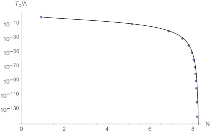
Figure 2: Dimensionless critical temperature ($T_{c}/\Lambda$) as a function of $N$ for $\Lambda=g^{2}$. The blue dots have been determined numerically, and agree very well with the semi-analytic prediction of Subsec. IV.4 (black curve).

IV.4 Semi-analytic approach

Given the previous numerical results, we need to understand the parametric dependence of $T_{c}$ on $N$ and $\Lambda/g^{2}$, as well as the nature of the transition $T_{c}\to 0$ that is seen around $N\sim 8.3$. With this aim, let us now develop an approximate approach for solving the gap equation. Since we are interested in small temperatures (in fact, vanishingly small near the putative transition), for our purpose it will be sufficient to work with the continuum approximation to the Matsubara sum,

$$\tilde{\Delta}(\omega)=\frac{1}{2N}\int_{\pi T_{c}}^{\infty}d\omega^{\prime}u(\omega,\omega^{\prime})\frac{\tilde{\Delta}(\omega^{\prime})}{A(\omega^{\prime})}\,.$$ (IV.29)

The lower integration limit takes into account that the fermionic Matsubara levels start at $\omega=\pi T$; the linearization is valid because we set $T=T_{c}$. Nonlinear effects will be discussed in Sec. V. Works with related methods include 2016PhRvL.117o7001W ; Wang:2017teb ; Abanov_2020 ; Wu_2020 .

The first key point is that $T_{c}$ appears to vanish for $N\gtrsim 8.3$. This is consistent with the $T=0$ analysis of the superconducting instability of Sec. III, were it not for the fact that both the RG and differential equation approaches give a slightly smaller value $N_{cr}=8$. This difference arises because the full eigenvalue problem (IV.22) – (IV.24) that determines $T_{c}$ includes nonlocal effects that are not taken into account in the local approximation. These arise from terms $m\neq n$ in the Matsubara sum (IV.22) or, equivalently, from regions in the integral (IV.29) with $\omega^{\prime}$ different from the external frequency. The difference between the local and nonlocal results is just of a few percent, but a more precise analytic determination of $N_{cr}$ is required in order to understand the transition between the normal and superconducting states.

One way to obtain $N_{cr}$ analytically is to approach $N\to N_{cr}$ from above, in which case $T_{c}\to 0$, and focus on the range $\omega<\Lambda$. Since the fermion dynamics here is dominated by the quantum critical behavior, we expect a power-law dependence for $\tilde{\Delta}(\omega)$. Neglecting subleading corrections from the Fermi-liquid range of the integral in (IV.29), the gap equation becomes

$$\tilde{\Delta}(\omega)\approx\frac{2}{3N}\,\int_{0}^{\Lambda}d\omega^{\prime}\left(\frac{1}{|\omega^{\prime}-\omega|^{1/3}}+\frac{1}{(\omega+\omega^{\prime})^{1/3}}\right)\frac{\tilde{\Delta}(\omega^{\prime})}{(\omega^{\prime})^{2/3}}$$ (IV.30)

From (III.24), we expect a power-law dependence $\tilde{\Delta}(\omega)\sim\omega^{-1/6}$ near the transition, so let us parametrize

$$\tilde{\Delta}(\omega)\approx\frac{1}{\omega^{\frac{1}{6}+\frac{\nu}{3}}}\;,\;\nu\ll 1\,.$$ (IV.31)

Performing the integral in the right hand side of (IV.30) with (IV.31) and small $\nu$, and matching with the left hand side, gives

$$N\approx 8.307+32.01\,\nu^{2}\,.$$ (IV.32)

Hence

$$\nu\approx\pm 0.51\sqrt{\frac{N}{8.307}-1}\,.$$ (IV.33)

The square root behavior is the smoking gun signature of the BKT transition: we find two real solutions –corresponding to the UV and IR fixed points (III.11) of the BCS coupling– which disappear and go off to the complex plane for $N<8.307$. We see then that the critical value from the local approximation is modified to

$$N_{cr}\approx 8.307$$ (IV.34)

due to nonlocal effects. Recently, Ref. 2019arXiv191201797C obtained an analytic expression $N(\nu)$ for all $\nu$; it agrees with (IV.34) at small $\nu$. For our purpose, (IV.33) will be sufficient.

Our approach now will be to derive a differential equation approximation to (IV.29), improved by the result (IV.34) in a way that we explain shortly. We will find that this provides a very good fit for the numerical results, as well as a physical understanding for the behavior of $T_{c}$.

The local approximation to (IV.29) gives again (III.18), but finite $T=T_{c}$ introduces two modifications: $A(\omega)$ now includes thermal effects from $\Sigma_{T}$ in (IV.7), and the infrared boundary condition becomes

$$\tilde{\Delta}^{\prime}(\pi T_{c})=0\,.$$ (IV.35)

This will fix $T_{c}$. Recall that at $T=0$ we had $\tilde{\Delta}^{\prime}(\omega=\Delta_{0})=0$ at the physical gap $\Delta_{0}$. In Fermi-liquid superconductivity, the physical gap and critical temperature are in fact the same up to pre-exponential factors. But will find that, due to NFL thermal effects encoded in $\Sigma_{T}$, there is a parametric suppression of $T_{c}$ compared to the gap. So it is important to distinguish both quantities.

As for the $T=0$ case, it is useful to use the dimensionless variable $x$ given by (III.21), for which we have

$$A(\omega)=\Lambda e^{-2x}(e^{-x}+1+e^{2(x-x_{T})})\,.$$ (IV.36)

The quantity $x_{T}$ is defined by

$$\Lambda_{T}=\Lambda e^{-3x_{T}}\,,$$ (IV.37)

and $\Lambda_{T}$ was given in (IV.11).

The differential equation together with the boundary conditions are

$$\tilde{\Delta}^{\prime}(x)-\tilde{\Delta}^{\prime\prime}(x)=\frac{\tilde{g}_{1}}{e^{-x}+1+e^{2(x-x_{T})}}\tilde{\Delta}(x)$$ (IV.38)

$$\tilde{\Delta}^{\prime}(x_{c})=0\,\,,\,\,\tilde{\Delta}(x\to-\infty)\sim e^{x}$$ (IV.39)

where $x_{c}$ is just $T_{c}$ in terms of the $x$-variable, $\pi T_{c}=\Lambda e^{-3x_{c}}$ and the second equation above corresponds to the boundary condition in the UV.

The strictly local approximation gives $\tilde{g}_{1}=2/N$ as in (III.21), (III.22); this would imply $N_{cr}=8$. Instead, here we have kept $\tilde{g}_{1}$ more general so that we can incorporate nonlocal effects. In order to reproduce (IV.34), we have to choose

$$\tilde{g}_{1}=\frac{1}{4}\frac{N_{cr}}{N}\approx\frac{1}{4}\frac{8.3}{N}\,.$$ (IV.40)

Although we won’t need further details, we remark that, following an approach similar to Abanov_2020 , such a modification can be incorporated by keeping a region $\omega^{\prime}$ around $\omega$ in the integral where $u(\omega,\omega^{\prime})$ is not simplified by the local approximation. Rather, the integral is evaluated by saddle point in this region.

It is now easy to solve (IV.38) and (IV.39) numerically, given (IV.40). The resulting $\tilde{\Delta}(\omega)$ is shown as the black curve in Fig. 2, exhibiting an excellent agreement with the numerical finite temperature data.

It remains to determine the parametric dependence of $T_{c}$ on $\Lambda/g^{2}$ and $N$. For this purpose, it is sufficient to construct approximate solutions in appropriate regimes of the frequency, subsequently imposing continuity and differentiability at the gluing points. There are three distinct regions: the high frequency regime $-\infty<x<0$, dominated by the first term in the denominator of (IV.38); the intermediate regime $0<x<x_{T}$, determined by the quantum NFL behavior (second term in the denominator of (IV.38)); and the low frequency region $x_{T}<x$, dominated by thermal effects from $\Sigma_{T}$ (third term in that denominator). The main effect of this last contribution is to suppress exponentially the right hand side of (IV.38), making the solution approach a constant for $x>x_{T}$.

All in all, the piecewise solution now reads

$$\tilde{\Delta}(x)\approx\left\{\begin{array}[]{lcc}e^{\frac{x}{2}}J_{1}(2\sqrt{\tilde{g}_{1}}e^{\frac{x}{2}})&,&-\infty<x<0\\ C_{1}e^{\frac{x}{2}}\cos\left(\sqrt{\tilde{g}_{1}-\frac{1}{4}}x+\phi\right)&,&0<x<x_{T}\\ D_{1}&,&x>x_{T}\end{array}\right.$$ (IV.41)

For high frequencies we have retained only the decaying solution $\Delta\sim\omega^{-1/3}$ as $\omega\to\infty$, as imposed by the UV boundary condition. The overall scale here is not fixed, since we are looking at the linearized problem. On the other hand, the constants $C_{1}$, $\phi$ and $D_{1}$ are fixed by imposing continuity of $\Delta(x)$ and $\Delta^{\prime}(x)$ at the matching points, thus becoming functions of $\tilde{g}_{1}$.

The main new effect is that the solution stabilizes to a constant value for $x>x_{T}$ or, equivalently, for $\omega<\Lambda_{T}$. This happens for frequencies in the range such that the self-energy is completely dominated by the thermal piece $\Sigma_{T}$. As a result, thermal effects shift the IR boundary condition (IV.35) from $x_{c}$ to $x_{T_{c}}<x_{c}$, namely

$$\tilde{\Delta}^{\prime}(\Lambda_{T_{c}})=0\,.$$ (IV.42)

This behavior was observed before in the $d=3-\epsilon$ analysis of Wang:2017teb ; the physical consequences will be here greatly amplified compared to Wang:2017teb because quantum and thermal effects are much stronger in $d=2$ dimensions.

The physical gap $\Delta_{0}$ is the frequency at which $\tilde{\Delta}(\omega)$ stabilizes to a constant, and hence here

$$\Delta_{0}=\Lambda_{T_{c}}\,.$$ (IV.43)

This scale sets the onset of superconductivity. The last step is to determine $T_{c}$ in terms of the parameters of the theory. For this, it is easiest to recognize that we have already solved an equivalent problem in (III.22) and (III.24) – we only need to replace $g_{1}$ there by the improved $\tilde{g}_{1}$ in (IV.40), as well as identify $x_{0}$ of that problem with $x_{T_{c}}$ in our current analysis. The result is

$$x_{T_{c}}\approx\frac{2\pi}{\sqrt{4\tilde{g}_{1}-1}}\,.$$ (IV.44)

Knowing $x_{T_{c}}$ determines $\Lambda_{T_{c}}=\Lambda e^{-3x_{T_{c}}}$. Recalling its expression (IV.11) in terms of the temperature then gives $T_{c}$, and furthermore plugging into (IV.43) fixes the gap. The final results are

$$\frac{T_{c}}{\Lambda} \approx \frac{4\pi}{\log\frac{g^{2}}{\lambda_{\phi}}}\,\frac{\Lambda}{g^{2}}\,\exp\left(-\frac{8\pi}{\sqrt{N_{cr}/N-1}}\right)$$

$$\frac{\Delta_{0}}{\Lambda} \approx \exp\left(-\frac{6\pi}{\sqrt{N_{cr}/N-1}}\right)\,.$$ (IV.45)

Let us highlight four consequences of these results.

• This reveals an infinite order BKT-type transition as $N\to N_{cr}$; conceptually, this is in agreement with previous RG and Eliashberg studies in $d=3-\epsilon$ at $T=0$ Raghu:2015sna ; Wang:2016hir and at finite $T$ Wang:2017teb . This analytic behavior is in excellent agreement with the numerical results, as illustrated above in Fig. 2.

• Both $T_{c}$ and $\Delta_{0}$ depend exponentially on a function of $N$. While the $N$-dependence shown in (IV.4) is corrected away from $N\sim N_{cr}$, the numerical results show large suppressions even for $N\sim 1$. This should be contrasted with the naive expectation that in $d=2$ the values of $(T_{c},\Delta_{0})$ should be determined by $\Lambda$ and/or $g^{2}$ with some power-law dependence but without exponentials. Instead, we have obtained a large suppression that comes from strong quantum NFL effects.

• Thermal fluctuations introduce a parametric scale separation $T_{c}\ll\Delta_{0}$ that originated from the premature stabilization of the gap at $\Lambda_{T_{c}}$. $T_{c}$ is exponentially smaller than $\Delta_{0}$, except at the smallest $N\sim 1$. On top of this, there is an extra suppression in $T_{c}$ by $(\Lambda/g^{2})$ compared to $\Delta_{0}$. The hierarchy $T_{c}/\Lambda_{0}\ll 1$ provides a distinct signature of non-Fermi liquid superconductivity.

• Finally, in the limit $\lambda_{\phi}/g^{2}\to 0$, we find $T_{c}/\Lambda\to 0$ from the inverse logarithm in (IV.4). This shows explicitly how large thermal corrections from virtual static bosons tend to destroy superconductivity.

Strictly at $N=1$ thermal effects cancel, as shown in Sec. IV.2. These results apply for $N>1$. They illustrate very explicitly the general points of Sec. II on the conceptual distinction between $N=1$ and $N>1$ in NFLs.

IV.5 Summary and phase diagram

This ends our analysis of superconductivity around $T=T_{c}$, so it is useful to summarize the picture that emerges for the NFL dynamics. A schematic phase diagram is presented in Fig. 3.

Figure 3: Schematic phase diagram, the lower half being the main focus of this work, i.e. temperatures below $\Lambda^{2}/g^{2}$. The red line represents the second-order transition to the superconducting state, with critical temperature well-approximated by (IV.4). The point $(T=0,N=N_{cr})$ where the transition line ends displays BKT criticality. Beyond that point, the system flows to a stable NFL with critical (finite) couplings.

For $N>N_{cr}$ the system does not superconduct, but rather displays a stable naked quantum critical point at $T=0$. The BCS coupling also reaches a stable fixed point. The finite $T$ dynamics of this normal state has been recently discussed in Damia:2020yiu . The traditional picture of a quantum critical region determined by $T=0$ scaling laws is strongly modified by thermal effects that become important at $T>\Lambda^{2}/g^{2}$ (the blue region in Fig. 3). In this range, the fermion Green’s function scales like $G_{F}\sim T^{-1/2}$ instead of $G_{F}\sim T^{-2/3}$.

At $N=N_{cr}$, numerical results are consistent with an infinite order transition, with BKT scaling (IV.4). Physically, the RG provides a compelling explanation: the IR stable QCP annihilates against an unstable fixed point. This is represented by the $\beta$-function (III.10).

For $N<N_{cr}$, the ground state is a superconductor. The line $T=T_{c}(N)$ of second order phase transitions ends at the BKT transition at $N=N_{cr}$. We have found that this NFL superconductor is quite different from BCS expectations. There is an important suppression both of $T_{c}$ and the physical gap $\Delta_{0}$ even for $N\sim 1$. Furthermore, a clear phenomenological signature is given by the parametric suppression $T_{c}\ll\Delta_{0}$ observed numerically and explained analytically in (IV.4).

It is quite plausible that the large $N$ results are not quantitatively correct down to $N\sim 1$. But we expect the previous qualitative picture to survive in this case. In fact, at small $N$ we expect stronger quantum corrections and hence further enhancement of NFL effects, but it would be interesting to analyze this further. This key distinction between $N=1$ and $N>1$ motivates future numerical analyses of this or related NFL models.

V Non-linear superconductivity and infrared divergences

So far we have studied the competition between NFL effects and superconductivity at finite temperature, by focusing on $T=T_{c}$ and linearizing the gap equation. In this last section we will analyze the full Schwinger-Dyson equations, including the nonlinear gap equation. The usual type of nonlinear solution obtains from extending the linearized solution of the previous section to $T<T_{c}$. The dynamics here is that expected from a gapped system with spontaneous symmetry breaking. Instead, our goal is to determine whether other solutions might exist at the nonlinear level.

There are two motivations to carry out this analysis. The first is that the linearized solution used a self-consistent thermal boson mass to cure the infrared divergences. However, one can envision that the superconducting gap itself could give rise to a bosonic mass and hence eliminate the thermal divergences. The dependence on the gap would then be necessarily non-analytic and requires solving the nonlinear Schwinger-Dyson equations. The other motivation comes from “first Matsubara law” solutions found in the closely related $\gamma$ model 2016PhRvL.117o7001W ; 2019PhRvB..99n4512W ; 2019arXiv191201797C ; Abanov_2020 ; Wu_2020 . These solutions are driven predominantly by superconducting gaps along the first few Matsubara modes, which is quite different from the linearized solution above. Our theory differs from that in 2016PhRvL.117o7001W ; 2019PhRvB..99n4512W ; 2019arXiv191201797C ; Abanov_2020 ; Wu_2020 by inclusion of thermal effects, but it is nevertheless natural to ask if similar solutions exist here.

This analysis will be more involved, so let us here summarize our findings and then describe the strategy we will follow. First, at sufficiently large $T$ (we make this precise below), we find that a gap does not develop at nonlinear level. In this case the mechanism for resolving IR divergences is still via a self-consistent boson mass as in Damia:2020yiu . This is fortunately consistent with the standard intuition that at high temperatures the normal state should be stable. On the other hand, at small temperatures we do find that a consistent solution with a nonlinear gap develops, and that this gives rise to a bosonic mass that is generically larger than the self-consistent contribution (IV.6). This provides then an interesting mechanism for resolution of thermal divergences. To determine the fate of this new branch of solutions, we analyze the Luttinger-Ward free energy, finding that this solution in fact has higher free energy than the normal state. As a result, we conclude that this solution does not appear to be relevant for the finite $T$ dynamics of the theory. Towards the end of the section we will comment on the connection with the nonlinear solution of 2016PhRvL.117o7001W ; 2019PhRvB..99n4512W ; 2019arXiv191201797C ; Abanov_2020 ; Wu_2020 .

V.1 Strategy

As discussed above, extending the linearized solution to $T<T_{c}$ will give a gapped superconducting state where $\Delta(\omega)$ stabilizes to $\Delta_{0}$ as $\omega\to 0$. The linearized solution relied on the thermal mass (IV.6) to make static boson exchanges finite. On the other hand, the bosonic mass $m^{2}$ also receives contributions from the gap, which at one loop read

$$m^{2}_{\Delta}=\frac{g^{2}k_{F}T}{2vN}\sum_{n=0}^{\infty}\frac{\tilde{\Delta}_{n}^{2}}{(A_{n}^{2}+\tilde{\Delta}^{2}_{n})^{3/2}}\,,$$ (V.1)

as derived in (A.21). It is then in principle possible to have a different branch of solutions at the nonlinear level if this mass contribution can become larger than (IV.6). So we will assume $m_{\Delta}^{2}\gg m_{b}^{2}$ and look for nontrivial nonlinear solutions.

From the dynamical exponent $z_{f}=3/2$ of the $T=0$ theory, we expect that in this new solution

$$\Sigma(\omega_{n})\sim\Lambda^{1/3}T^{2/3}\;,\;\tilde{\Delta}(\omega_{n})\sim\Lambda^{1/3}T^{2/3}\,,$$ (V.2)

for $T<\Lambda$, up to small corrections suppressed by $1/\Lambda$. This should be contrasted with the results in previous sections, where the violation of the $T=0$ scalings was allowed because of the dangerously irrelevant coupling $\lambda_{\phi}$. In this section, we are assuming that effects from $\lambda_{\phi}$ are subleading, since we are interested in new nonlinear solutions.

Having understood what type of temperature scaling we are after, it remains to obtain the dependence on the Matsubara level $n$. It is convenient to switch to dimensionless variables (IV.21). We look for solutions of the nonlinear Schwinger-Dyson equations,

$$\hat{A}_{n} = \hat{\omega}_{n}+\hat{f}_{n}\frac{\hat{A}_{n}}{\sqrt{\hat{A}_{n}^{2}+\hat{\Delta}_{n}^{2}}}+\xi\sum_{m=0}^{\infty}K^{-}_{nm}\frac{\hat{A}_{m}}{\sqrt{\hat{A}_{m}^{2}+\hat{\Delta}_{m}^{2}}}$$

$$\hat{\Delta}_{n} = \frac{1}{N}\hat{f}_{n}\frac{\hat{\Delta}_{n}}{\sqrt{\hat{A}_{n}^{2}+\hat{\Delta}_{n}^{2}}}+\frac{1}{N}\xi\sum_{m=0}^{\infty}K^{\pm}_{nm}\frac{\hat{\Delta}_{m}}{\sqrt{\hat{A}_{m}^{2}+\hat{\Delta}_{m}^{2}}}$$

derived in Appendix A, see (A.4). The function $\hat{f}_{n}$ is a generalization of $\Sigma_{T}$ in (IV.9) that includes the SC gap,

$$\hat{f}_{n}\equiv\frac{g^{2}}{2\pi^{3}T}\frac{\cosh^{-1}\left(\frac{1}{v}\sqrt{\frac{\hat{A}_{n}^{2}+\hat{\Delta}_{n}^{2}}{\hat{m}^{2}}}\right)}{\sqrt{\hat{A}_{n}^{2}+\hat{\Delta}_{n}^{2}-v^{2}\hat{m}^{2}}}\,,$$ (V.4)

see (A.28).

Therefore we need to solve the coupled equations (V.1), which include nonlinear terms both from the square roots there, as well as from the infrared contributions encoded in $\hat{f}_{n}$. This is in general quite hard, because we are dealing with an infinite number of coupled nonlinear equations. We will look for these solutions numerically by truncating to a finite number of Matsubara levels. But before doing this, we will show that the full solution is dominated by the first Matsubara modes. This is similar to the first Matsubara law solution of 2016PhRvL.117o7001W ; 2019PhRvB..99n4512W ; 2019arXiv191201797C ; Abanov_2020 ; Wu_2020 , but there are differences and we will compare with those works in Sec. V.5.

So we obtain the solution explicitly keeping only the first two modes, and then extend it to include additional Matsubara frequencies. While this is approximate (and will be later on improved with numerical results), it allows us to extract the main physical properties of this nonlinear regime.

V.2 Approximate truncated solution

The Schwinger-Dyson equations restricted to $n=0$ (i.e. the first Matsubara frequencies $\pm\pi T$) read

$$\hat{A}_{0} = \hat{\omega}_{0}+(\hat{f}_{0}-\xi)\,\frac{\hat{A}_{0}}{\sqrt{\hat{A}_{0}^{2}+\hat{\Delta}_{0}^{2}}}+\xi$$

$$\hat{\Delta}_{0} = \frac{1}{N}(\hat{f}_{0}+\xi)\,\frac{\hat{\Delta}_{0}}{\sqrt{\hat{A}_{0}^{2}+\hat{\Delta}_{0}^{2}}}\,.$$ (V.5)

Here $\hat{f}_{0}$ is given by (V.4) with mass restricted to the first mode,

$$\hat{m}^{2}\approx\frac{g^{2}k_{F}}{2\pi^{3}vNT^{2}}\frac{\hat{\Delta}_{0}^{2}}{(\hat{A}_{0}^{2}+\hat{\Delta}^{2}_{0})^{3/2}}\,.$$ (V.6)

We also note the last term $\xi$ in the equation for $\hat{A}_{0}$ – it is the NFL self-energy part that comes from $\sum_{m\geq 1}K^{-}_{mn}$ in (V.1) after setting $\hat{\Delta}_{m\geq 1}=0$ there.

At large $N$, we find an approximate solution by neglecting $\hat{f}_{0}$,

$$\hat{A}_{0}\approx\frac{1+\xi}{1+N}\,\,,\,\,\hat{\Delta}_{0}\approx\sqrt{\frac{\xi^{2}}{N^{2}}-\left(\frac{1+\xi}{1+N}\right)^{2}}\,.$$ (V.7)

This exists as long as the discriminant is positive, that is

$$\xi>N\,.$$ (V.8)

From the definition of $\xi$ given in (IV.15), this defines a temperature scale $T_{NL}$

$$T_{NL}\approx\frac{4}{27\pi}\,\frac{\Lambda}{N^{3}}$$ (V.9)

so that the nonlinear solution exists for any $N$ at sufficiently low temperatures

$$T<T_{NL}\,.$$ (V.10)

In this range, the solution approximates to

$$\hat{A}_{0}\approx\frac{\xi}{N}\;,\;\hat{\Delta}_{0}^{2}\approx 2\frac{\xi^{2}}{N^{3}}\,,$$ (V.11)

or, translating to the original dimensionful quantities,

$$A_{0}\approx\frac{1}{3N}\Lambda^{1/3}(2\pi T)^{2/3}\;,\;\tilde{\Delta}_{0}=\frac{\sqrt{2}}{3N^{3/2}}\Lambda^{1/3}(2\pi T)^{2/3}\,.$$ (V.12)

This agrees with the expected scaling (V.2) of the $T=0$ theory.

We see that the gap is subdominant compared to $\hat{A}_{0}$, and one can verify that the initial hypothesis $\hat{f}_{0}\ll\xi$ is consistently satisfied. We will discuss shortly what happens as $\xi\to N$. In obtaining this solution, we have neglected the thermal boson mass and contributions from higher Matsubara modes. We now argue that this is justified.

From (V.6) and (IV.6), the ratio between the gap-induced and thermal boson masses is

$$\frac{m^{2}_{\Delta}}{m^{2}_{b}}\approx\frac{g^{2}k_{F}}{v\lambda_{\phi}N}\frac{1}{\Lambda^{1/3}T^{2/3}}\approx\frac{g^{2}k_{F}}{v\lambda_{\phi}\Lambda N}\xi^{2}\,.$$ (V.13)

Since $\xi>N$ here, the thermal mass can be neglected as long as

$$\frac{\lambda_{\phi}}{g^{2}}<N\frac{k_{F}}{v\Lambda}\,.$$ (V.14)

This is easily satisfied because $N>1$ and $k_{F}\gg\Lambda$.

Regarding contributions from the higher Matsubara modes $\hat{\Delta}_{n}$, we note that they cannot be strictly zero because $\hat{\Delta}_{0}$ sources them. Indeed, keeping only $\hat{\Delta}_{0}$ in the right hand side of (V.1) gives a nonvanishing result

$$\hat{\Delta}_{n}\approx\frac{\xi}{N}{K}^{+}_{n0}\frac{\hat{\Delta}_{0}}{\sqrt{\hat{A}_{0}^{2}+\hat{\Delta}_{0}^{2}}}\,.$$ (V.15)

In order to evaluate the backreaction of $\hat{\Delta}_{n}$ on $\hat{\Delta}_{0}$, we need $\hat{A}_{n}$. Since already $\hat{\Delta}_{0}$ was much smaller than $\hat{A}_{0}$, we can neglect the gap altogether in the Schwinger-Dyson equation for the fermion self-energy, obtaining

$$\hat{A}_{n\geq 1}=\hat{\omega}_{n}+\xi\sum_{m=0}^{\infty}K^{-}_{nm}=\hat{\omega}_{n}+\hat{\Sigma}_{\rm NFL}^{n}$$ (V.16)

where $\hat{\Sigma}_{\rm NFL}^{n}=(\pi T)^{-1}{\Sigma_{\text{NFL}}}(\omega_{n})$ with ${\Sigma_{\text{NFL}}}(\omega_{n})$ given in (IV.8). As happened above with $\hat{f}_{0}$, effects from $\hat{f}_{n}$ are also negligible, and that is why we have not included such thermal self-energy terms here. Using (V.15) and (V.16), the terms with $m\geq 1$ give a relative contribution to the $n=0$ gap equation

$$\frac{\delta\hat{\Delta}_{0}}{\tilde{\Delta}_{0}}\approx\frac{\xi}{N}\sum_{m\geq 1}\frac{(K^{+}_{0m})^{2}}{\hat{A}_{m}}\,.$$ (V.17)

Since $\hat{A}_{m}\sim\xi m^{2/3}$ for $m\geq 1$, and the sum is convergent, this is therefore suppressed in the large $N$ limit, as promised.

It remains to determine what happens as $\xi\to N$. In this limit, $\hat{f}_{0}$ can no longer be neglected, because it diverges when $\hat{\Delta}_{0}\to 0$ as predicted by (V.7). So $\hat{f}_{0}\ll\xi$ will break down somewhere before $\xi=N$. Therefore, thermal effects encoded in $\hat{f}_{0}$ (and the $\hat{f}_{n}$ more generally) begin to play an important role. The system of equations (V.2) does not admit a simple analytic solution in this case. But it is not hard to solve it numerically. The basic outcome is that the solution still ceases to exist at a value of order $\xi\approx N$, but the main difference is that this happens at a finite $\hat{\Delta}_{0}$, and not at $\hat{\Delta}_{0}=0$ as in (V.7). This can be seen from the contour plots of the two equations (V.2) in the $(\hat{A}_{0},\hat{\Delta}_{0})$ plane. An example is given in Fig. 4. This reveals three solutions. The first one has $\hat{\Delta}_{0}=0$ and $\hat{A}_{n}$ is the usual normal state result; in the figure, $\hat{\Delta}_{0}=0$ appears as the constant orange line at the bottom, which intersects the contour line of the $\hat{A}$ equation to the far right. This is not shown here because we focus on the range with nonlinear solutions in the plot. Besides the normal state solution, this reveals two other nonlinear solutions, from the two contour intersections in the figure. As $T\to T_{NL}$ the two solutions annihilate, at this order. This happens at finite $\hat{\Delta}_{0}$ as seen in the plot. It would be interesting to understand in more detail this mechanism of annihilation, but this is outside the scope of this work (especially given that the solution will not be thermodynamically favored).

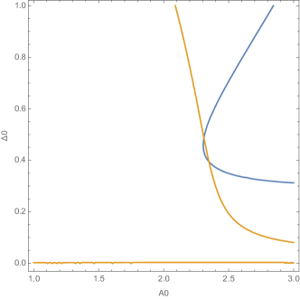
Figure 4: Contour plots eq$=0$ for the $A$ equation (blue) and gap equation (orange) for $T=3.1\times 10^{-9},N=10,g=M_{D}=1$, with the two solutions annihilating.This happens at a nonzero value of $\hat{\Delta}_{0}$. The constant $\hat{\Delta}_{0}=0$ line at the bottom intersects with the blue contour (the $\hat{A}$ equation) for much larger values of $\hat{A}_{0}$, not shown here.

To summarize, we have found a nonlinear solution at $T<T_{NL}$, where the gap has the profile (V.7) and (V.15). In this solution, the thermal boson mass is subdominant due to (V.14), and the formation of a gap provides a nonperturbative resolution of thermal divergences. This solution exists even at $N>N_{cr}$, for which the linearized analysis predicts no superconducting instability. The solution disappears discontinuously for $T\to T_{NL}$. It remains to determine if it is energetically favorable compared to the normal state. We will analyze this point in Subsec. V.4. But before turning to this, let us present numerical results for the complete Schwinger-Dyson equations that verify our current approach.

V.3 Numerics

The main conclusions from the previous analysis, namely the scaling (V.2) and the disappearance of the nonlinear solution as $T\to T_{NL}$, have been verified numerically. We have done this using numerical methods for finding roots of nonlinear systems. We solve the non-linear system (V.1) up to a given maximum frequency number $n_{max}$ and check convergence by varying this parameter. The truncated solution is used as an input for local searches of solutions in the full system.

An example is presented in Fig. 5. We chose $N=20$, so we expect the truncated result to give a good approximation, and indeed, this is what we find. Decreasing $N$ but still keeping $T$ low gives solutions that start to deviate from the truncated approximation, but the basic $T^{2/3}$ scaling of $\tilde{\Delta}_{n}$ is respected, as expected.

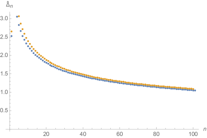
Figure 5: Numerical solution $\hat{\Delta}_{n}$ to (V.1) with $n_{max}=100$ (dots in blue), and truncated solution (orange). The parameters are $N=20,\,\Lambda=g^{2}=1,\lambda_{\phi}=1/10,T=10^{-8}$.

Increasing the temperature, the numerical solution ceases to exist for $T\sim T_{NL}$ as in (V.9). This is consistent with the results from the truncation in the previous section. It should be stressed that we have used local search methods; global methods are much more demanding and would require a different level of numerical analysis, such as that provided by neural networks. So, while at this stage we cannot forbid the existence of other nonlinear solutions, all our results converge to suggest that this is unlikely. Developing efficient methods for solving nonlinear Schwinger-Dyson equations would be very interesting.

V.4 Thermodynamic fate of the solution

We have found that accounting for non-linear effects leads to an alternative self-consistent solution to the Schwinger-Dyson equations. This solution is quite different from the normal state at $T>T_{c}$; it involves a mass term induced by fermionic loops in the presence of a self-consistent gap profile. The physical significance of this solution is not completely clear, particularly regarding the nature of global symmetry breaking. There are some proposals that similar first-Matsubara law solutions could describe a pseudogap state Abanov_2020 .

In the regime $T_{c}<T<T_{NL}$ where the normal state and nonlinear gap solutions exist, one of them will be energetically preferred. We will now address this, by evaluating their free energies with the Luttinger-Ward functional LuttingerWard:1960 ; Benlagra:2011 ; ChubukovHaslinger:2003 .

Let us focus on the free energy contribution from the Fermi surface (see Appendix B)

$$F_{f}=-\frac{NTk_{F}}{v}\sum_{n=0}^{\infty}\left(\sqrt{A_{n}^{2}+\tilde{\Delta}_{n}^{2}}+\frac{|\omega_{n}||A_{n}|}{\sqrt{A^{2}_{n}+\tilde{\Delta}_{n}^{2}}}\right)\,.$$ (V.18)

The main outcome from our previous results is that the normal state has $A_{n}\sim T^{1/2}$ over a broad range of Matsubara frequencies, while the nonlinear gapped state respects the $T=0$ scaling and hence both $A_{n}$ and $\tilde{\Delta}_{n}$ scale like $T^{2/3}$. Therefore,

$$F_{gapped}-F_{normal}\approx-\frac{NTk_{F}}{v}\left(\gamma_{0}\frac{T^{2/3}\Lambda^{1/3}}{N}-\gamma_{1}\sqrt{g^{2}T}\right)\,,$$ (V.19)

with $\gamma_{0}$ and $\gamma_{1}$ order one numerical constants that depend on the particular frequency profiles, but are approximately independent on $T$.

The different temperature scaling of both regimes implies that the nonlinear gapped state is stable only at sufficiently high temperatures,

$$\frac{T}{\Lambda}\gtrsim\left(\frac{g^{2}}{\Lambda}\right)^{3}N^{6}\,,$$ (V.20)

where we are keeping implicit some $O(1)$ numerical factors. On the other hand, this state only appears for $T<T_{NL}$ as in (V.10). Combining both conditions, we obtain that the gapped state will then exist and be energetically preferred only if

$$\frac{\Lambda}{g^{2}}\gtrsim N^{3}\,,$$ (V.21)

again up to $O(1)$ factors. This does not occur in general, because $\Lambda$ is a dynamical scale generated below $g^{2}$, that is $\Lambda<g^{2}$.

This discussion has incorporated only the parametric dependence on $N,T,\Lambda,g^{2}$, leaving some numerical constants undetermined. We have evaluated (V.19) on example solutions, finding agreement with this parametric analysis.

So far we have taken into account the fermionic free energy, but the bosonic sector also contributes. The non-static modes are approximately the same in the normal and gapped state, so only the static mode contributes to the energy difference. The bosonic free energy is evaluated in detail in Appendix B, and the outcome is similar to that in the fermionic sector: the conditions that the bosonic free energy in the gapped state is smaller than in the normal state, together with $T<T_{NL}$, force the theory into a regime of parameters that is not physically realized.

To summarize, the nonlinear gapped state of Sec. V.2 and V.3 is energetically disfavored compared to the normal state in the regime $T<T_{NL}$ where it exists. The dynamics and phase structure is then that of Sec. IV.

V.5 Comparing with the “first Matsubara law” solution

Let us end our analysis by comparing the previous nonlinear gapped state with the “first Matsubara law” solution of 2016PhRvL.117o7001W ; 2019PhRvB..99n4512W ; 2019arXiv191201797C ; Abanov_2020 ; Wu_2020 . These works solve gap equations that are similar to (IV.2), but dropping $m=n$ contributions from virtual static bosons. In the procedure leading to (IV.20), this amounts to setting $N=1$ in the definition of $\bar{A}(\omega_{n})$ there, but keeping the overall $1/N$ in the gap equation. We don’t know of a field theory construction that gives this; instead, the motivation in this line of research is to understand the physics of the $N=1$ theory but artificially decreasing the strength of the pairing instability in order to reveal NFL effects. As we have stressed in previous sections, in our work the parameter $N$ is physical (see Sec. II), and affects simultaneously the pairing strength and the thermal corrections.

Despite this difference, the nonlinear gap profile we have found shares some similarities with the first Matsubara law solution. The basic reason for this is that thermal effects (neglected from the start in 2016PhRvL.117o7001W ; 2019PhRvB..99n4512W ; 2019arXiv191201797C ; Abanov_2020 ; Wu_2020 ) are also very small in our case when $T\ll T_{NL}$. This was explained in Sec. V.2 , where the $\hat{f}_{n}$ were indeed found to be negligible if $T\ll T_{NL}$. The basic properties of the two solutions then agree at sufficiently small temperatures. Not coincidentally, these works also found a transition temperature for the first Matsubara law solution that behaves like our $T_{NL}$.

However, the dynamics and phase diagram in both approaches are quite different because, by not including thermal effects, the authors of 2016PhRvL.117o7001W ; 2019PhRvB..99n4512W ; 2019arXiv191201797C ; Abanov_2020 ; Wu_2020 found that the gapped first Matsubara law state is energetically preferred. In contrast, this state is energetically disfavored in our setup, precisely because thermal terms have a different parametric scaling with temperature, see (V.19). Superconductivity in our case only occurs for $N<N_{cr}$ and is driven by the linearized solution of Sec. IV. The details about how the gapped state disappears as $T\to T_{NL}$ are also different since these are sensitive to thermal static contributions as in Fig. 4.

VI Conclusions

In this work we have determined the consequences from virtual static bosons on superconductivity in NFLs. Motivated by different models, we identified a parameter $N$ that measures the ratio between self-energy and gap renormalizations. Thermal contributions from such static modes cancel only when $N=1$, while for any $N>1$ they are nonzero, violate quantum-critical scaling and dominate at small temperature. We performed a detailed analysis for a Fermi surface coupled to massless Landau damped bosons in $d=2$ space dimensions, where $N$ comes from a global $SU(N)$ symmetry. For $N>N_{cr}\sim 8$, the normal state is stable under superconductivity, leading to a naked quantum critical point at $T=0$, which features critical pairing fluctuations. An infinite order transition to superconductivity appears as $N\to N_{cr}$, with the critical temperature $T_{c}$ and the gap $\Delta_{0}$ displaying BKT scaling. The superconducting phase arises then for $N<N_{cr}$ and $T<T_{c}$. Superconductivity exhibits strong non-Fermi liquid deviations from the usual BCS results; quantum corrections lead to an exponential suppression of $T_{c}$ and $\Delta_{0}$, and thermal effects give rise to a parametric hierarchy $T_{c}\ll\Delta_{0}$. A summary of the phase diagram can be found in Fig. 3 above.

Let us suggest some directions of future research that are motivated by these results. We analyzed the role of thermal effects from static modes in a specific class of NFLs, but our basic conclusions regarding their effects when $N>1$ are likely more general. It would then be interesting to revisit other models of NFLs which feature an $N>1$, and include exchange of static modes at finite temperature. We suggest that this leads to a distinction between NFLs where superconductivity is enhanced ($N=1$) and others where it is suppressed ($N>1$), even with the same type of coupling to bosonic modes. This adds to the distinction between models with order parameters and models with emergent $U(1)$ gauge fields found in Metlitski . We also plan to extend our results to models with more general dynamical exponent $z_{f}$. These quantum critical points cover quite different phenomenology and arise also from semi-holographic constructions.

Finally, it would be interesting to further develop strong-coupling methods to cope with two-dimensional models with $N\sim 1$, which do not have a small-parameter expansion. Our predictions of the qualitative difference between $N=1$ and $N>1$ are encouraging in this direction, because we are finding that $N$ does not need to be too large in order to observe dramatic NFL effects. Models with moderate $N$ could reasonably be studied numerically in the near future, particularly given recent developments in Monte-Carlo methods Schattner2016 ; 2017PNAS..114.4905L ; Berg2019 ; liu2019itinerant ; klein2020normal ; Xu:2020tvb .

Appendix A Schwinger-Dyson equations

This Appendix presents the derivation of the Schwinger-Dyson equations, together with approximate expressions used in the main text.

A.1 Notation and conventions

In the Nambu-Gorkov basis for the fermionic fields we have

$$\Psi_{i}=\left(\begin{array}[]{c}\psi_{i}(p)\\ \psi_{i}(-p)^{\dagger}\end{array}\right)\,,$$ (A.1)

where we are collectivelly denoting $p=(\omega,\vec{p})$ and $i$ denotes the $SU(N)$ flavor index. The term in the action accounting for the gap coupling is then

$$\Psi^{T}_{i}(p)\tilde{\Delta}^{M}_{ij}\Psi_{j}(-p^{\prime})\,,$$ (A.2)

with the pairing gap matrix defined as

$$\tilde{\Delta}^{M}=\left(\begin{array}[]{cc}\tilde{\Delta}_{ij}(p-p^{\prime})&0\\ 0&\tilde{\Delta}^{\dagger}_{ij}(p-p^{\prime})\end{array}\right)\,.$$ (A.3)

The Green’s function reads

$${\cal G}_{ij}=\langle\Psi_{i}(p)\Psi_{j}(p)^{\dagger}\rangle=\left(\begin{array}[]{cc}G_{ij}(p)&\tilde{G}_{ij}(p)\\ -\tilde{G}_{ij}(p)^{*}&G_{ij}(p)^{*}\end{array}\right)\,,$$ (A.4)

where

$$G_{ij}(p) = \delta_{ij}\frac{\varepsilon_{p}+iA(p)}{\varepsilon_{p}^{2}+A(p)^{2}+|\tilde{\Delta}(p)|^{2}}\,,$$ (A.5)

$$\tilde{G}_{ij}(p) = \frac{\tilde{\Delta}_{ij}(p)}{\varepsilon_{p}^{2}+A(p)^{2}+|\tilde{\Delta}(p)|^{2}}\,,$$ (A.6)

and we recall that $A(p)=\omega+\Sigma(p)$.

Throughout this work, we will consider the following simple symmetry breaking pattern for the pairing vertex,

$$\tilde{\Delta}_{ij}(p)=\tilde{\Delta}(p)J_{ij}\,,\;\;J_{ij}=\left(\begin{array}[]{cc}0&{\mathbb{I}}_{N/2}\\ -{\mathbb{I}}_{N/2}&0\end{array}\right)\,.$$ (A.7)

In addition, for the bosonic propagator we have

$$D^{-1}_{ij,kl}(\Omega,q)=\delta_{il}\delta_{jk}\left(q^{2}+M_{D}^{2}\frac{|\Omega|}{q}\right)+\Pi_{ij,kl}(\Omega,q)\,.$$ (A.8)

The leading contributions to the bosonic self-energy are of the form $\Pi_{ij,kl}\sim\delta_{il}\delta_{jk}$, so we can write

$$D^{-1}_{ij,kl}(\Omega,q) = \delta_{il}\delta_{jk}D^{-1}(\Omega,q)\,,$$

$$D^{-1}(\Omega,q) = q^{2}+M_{D}^{2}\frac{|\Omega|}{q}+\Pi(\Omega,q)\,.$$ (A.9)

A.2 Schwinger-Dyson-Eliashberg equations

As shown in Damia:2020yiu , for a vanishing gap function, self-interactions of static (zero frequency) bosonic modes have to be accounted for in order to get a self-consistent solution free of IR singularities. For higher frequencies, this interaction becomes irrelevant due to the $z_{b}=3$ scaling induced by Landau damping and we will ignore it. The effective action for the static mode reads

$$S_{\Omega_{n}=0}=\int\frac{d^{2}q}{(2\pi)^{2}}\frac{1}{2}\,\text{tr}\,(\tilde{\phi}_{q}q^{2}\tilde{\phi}_{-q})+\frac{\lambda_{\phi}T}{8N}\int\prod_{i=1}^{3}\frac{d^{2}q_{i}}{(2\pi)^{2}}\,\text{tr}(\tilde{\phi}_{q_{1}}\tilde{\phi}_{q_{2}}\tilde{\phi}_{q_{3}}\tilde{\phi}_{-q_{1}-q_{2}-q_{3}})\,,$$

with $\tilde{\phi}(q)\equiv T^{1/2}\phi(\Omega_{n}=0,q)$. A scaling analysis shows that the coupling $\lambda_{\phi}T$ becomes relevant at low energies and momenta $q<(2\pi TM_{D}^{2})^{1/3}$. The cutoff here is set by the gap to higher Matsubara modes. For a more detailed treatment we refer the reader to Damia:2020yiu .

Working out the contractions over flavor indices and keeping the leading terms, the self-consistent equations ignoring vertex corrections are

$$\Pi(\Omega_{n},q) = \frac{g^{2}T}{N}\sum_{m}\int\frac{d^{2}p}{(2\pi)^{2}}\,G(p,\omega_{n})G(p+q,\Omega_{m}+\omega_{n})+\delta_{n,0}\lambda_{\phi}T\int\frac{d^{2}p}{(2\pi)^{2}}D(p,0)$$ (A.10)

$$i\Sigma(p,\omega_{n}) = g^{2}T\sum_{m}\int\frac{d^{2}q}{(2\pi)^{2}}G(q,\omega_{m})D(p-q,\omega_{n}-\omega_{m})$$ (A.11)

$$\tilde{\Delta}(p,\omega_{n}) = \frac{g^{2}T}{N}\sum_{m}\int\frac{d^{2}q}{(2\pi)^{2}}\tilde{G}(q,\omega_{m})D(p-q,\omega_{n}-\omega_{m})\,.$$ (A.12)

Recall that $\tilde{G}$ was defined in (A.6). We have neglected contributions from $\tilde{G}$ to the bosonic self-energy equation (A.2) because they are of order $N^{-2}$. Index contractions using the pattern (A.7) give the $1/N$ factor in (A.15). We do not neglect this $1/N$ effect because it is the leading contribution to the gap; moreover, if the gap develops, it is always a relevant deformation to the critical point and hence becomes important at long distance. The above equations can be alternatively obtained by minimizing the Luttinger-Ward free energy functional as shown in Appendix B.

Finally, plugging (A.5), (A.6) and (A.9) we get

$$\Pi(\Omega_{m},q) = \frac{g^{2}}{N}T\sum_{n}\,\int\frac{d^{2}p}{(2\pi)^{2}}\,\frac{iA(\omega_{n})+\varepsilon_{p}}{A(\omega_{n})^{2}+|\tilde{\Delta}(\omega_{n})|^{2}+\varepsilon_{p}^{2}}\frac{iA(\omega_{n}+\Omega_{m})+\varepsilon_{p+q}}{A(\omega_{n}+\Omega_{m})^{2}+|\tilde{\Delta}(\omega_{n}+\Omega_{m})|^{2}+\varepsilon_{p+q}^{2}}$$

$$+\,\,\delta_{n,0}\lambda_{\phi}T\int\frac{d^{2}p}{(2\pi)^{2}}\frac{1}{p^{2}+\Pi(0,p)}\,,$$

$$i\Sigma(\omega_{n}) = g^{2}T\sum_{m}\int\frac{d^{2}q}{(2\pi)^{2}}\frac{1}{q^{2}+M_{D}^{2}\frac{|\omega_{n}-\omega_{m}|}{q}+\Pi(\omega_{m}-\omega_{n},q)}\,\frac{iA(\omega_{m})+\varepsilon_{p+q}}{A(\omega_{m})^{2}+|\tilde{\Delta}(\omega_{m})|^{2}+\varepsilon_{p+q}^{2}}$$ (A.14)

$$\tilde{\Delta}(\omega_{n}) = \frac{g^{2}}{N}T\sum_{m}\int\frac{d^{2}q}{(2\pi)^{2}}\frac{1}{q^{2}+M_{D}^{2}\frac{|\omega_{n}-\omega_{m}|}{q}+\Pi(\omega_{m}-\omega_{n},q)}\,\frac{\tilde{\Delta}(\omega_{m})}{A(\omega_{m})^{2}+|\tilde{\Delta}(\omega_{m})|^{2}+\varepsilon_{p+q}^{2}}\,.$$ (A.15)

We have already made explicit our assumption that the fermion self-energy and gap only depend on the frequency, as explained in the main text.

A.3 Bosonic mass

Let us first focus on the equation for the bosonic self-energy (A.2), which we rewrite here again after expanding the fermionic energy near the Fermi surface ($\varepsilon_{p}\approx vp_{\perp}$)

$$\Pi(\Omega_{n},q)= \frac{g^{2}k_{F}T}{N}\sum_{m}\int\frac{dp_{\perp}d\theta}{(2\pi)^{2}}\frac{(iA_{m}+vp_{\perp})(iA_{n+m}+v(p_{\perp}+q\cos\theta))}{(A_{m}^{2}+\tilde{\Delta}_{m}^{2}+(vp_{\perp})^{2})(A_{n+m}^{2}+\tilde{\Delta}_{n+m}^{2}+v^{2}(p_{\perp}+q\cos\theta)^{2})}$$ (A.16)

$$+ \delta_{n,0}\lambda_{\phi}T\int\frac{d^{2}p}{(2\pi)^{2}}\frac{1}{p^{2}+\Pi(0,p)}\,,$$

For non-zero frequency modes, the gap contribution is negligible and the remaining integral leads to a term of the same form as the UV Landau damping in (A.9), but suppressed by $1/N$. This can be neglected.

For the static modes, the situation is more subtle. At high enough temperatures we expect to have a disordered phase, so let us start by assuming a vanishing gap, i.e. $\{\tilde{\Delta}_{n}\}=\{0\}$. As described in Damia:2020yiu , in that case the contribution from the first line in (A.16) vanishes for zero external frequency. So the Schwinger-Dyson equation gives a self-consistent equation for a boson thermal mass,

$$\{\tilde{\Delta}_{n}\}=\{0\}\,\,\Rightarrow\,\,\Pi(0,q)\approx m^{2}_{b}=\frac{\lambda_{\phi}T}{2\pi}\int\frac{p\,dp}{p^{2}+m^{2}_{b}}\,,$$ (A.17)

with approximate solution

$$m_{b}^{2}\approx\frac{\lambda_{\phi}T}{4\pi}\,\,\log\left(4\pi\frac{(2\pi TM_{D}^{2})^{2/3}}{\lambda_{\phi}T}\right)\,.$$ (A.18)

The inclusion of the thermal mass (A.18) leads to the normal state described in Damia:2020yiu and reviewed in Sec. IV.1.

However, at low temperatures, a solution with non-trivial gap might develop, so we need to consider that case as well. For simplicity, we assume that in such a case, the first line in (A.16) dominates, such that we can neglect the effect of static mode self-interactions. This assumption is shown to be consistently satisfied by the solutions found in Sec. V. In this case,

$$\{\tilde{\Delta}_{n}\}\neq\{0\}\,\Rightarrow\,\Pi(0,q) \approx \frac{g^{2}k_{F}T}{(2\pi)^{2}}\sum_{n}\int dp_{\perp}d\theta\frac{(iA_{n}+vp_{\perp})(iA_{n}+v(p_{\perp}+q\cos\theta))}{(A_{n}^{2}+\tilde{\Delta}_{n}^{2}+(vp_{\perp})^{2})(A_{n}^{2}+\tilde{\Delta}_{n}^{2}+v^{2}(p_{\perp}+q\cos\theta)^{2})}\,,$$ (A.19)

$$= \frac{g^{2}k_{F}T}{4vN}\sum_{n}\frac{\tilde{\Delta}_{n}^{2}}{(A_{n}^{2}+\tilde{\Delta}^{2}_{n})\sqrt{A_{n}^{2}+\tilde{\Delta}^{2}_{n}+(vq/2)^{2}}}\,,$$ (A.20)

where, in going to the second line,we performed the momentum integration. As we are interested in the limit of small momentum, we take $q\to 0$ in the last expression above, thus obtaining

$$\Pi(0,q)\approx m^{2}_{\Delta}=\frac{g^{2}k_{F}T}{4vN}\sum_{n}\frac{\tilde{\Delta}_{n}^{2}}{(A_{n}^{2}+\tilde{\Delta}^{2}_{n})^{3/2}}\,.$$ (A.21)

(As we just discussed, for this to be self-consistent we must check that $m^{2}_{\Delta}\gg m_{b}^{2}$ once the corresponding solution is obtained, as we do in Sec. V.)

A.4 Momentum integrals

Now we turn to the remaining Schwinger-Dyson-Eliashberg equations (A.14) and (A.15). Plugging the propagators (A.5), (A.6) and (A.9), and using the integral

$$\int_{0}^{2\pi}d\theta\frac{a+b\cos\theta}{c^{2}+(b\cos\theta)^{2}}=\frac{2\pi a}{|c|\sqrt{c^{2}+b^{2}}}$$ (A.22)

we obtain

$$\Sigma(\omega_{n}) = \frac{g^{2}T}{2\pi}\sum_{m}\frac{A(\omega_{m})}{\sqrt{A(\omega_{m})^{2}+\tilde{\Delta}(\omega_{m})^{2}}}\int qdq\frac{D(i\omega_{n}-i\omega_{m},q)}{\sqrt{A(\omega_{m})^{2}+\tilde{\Delta}(\omega_{m})^{2}+(vq)^{2}}}\,,$$ (A.23)

$$\tilde{\Delta}(\omega_{n}) = \frac{1}{N}\frac{g^{2}T}{2\pi}\sum_{m}\frac{\tilde{\Delta}(\omega_{m})}{\sqrt{A(\omega_{m})^{2}+\tilde{\Delta}(\omega_{m})^{2}}}\int qdq\frac{D(i\omega_{n}-i\omega_{m},q)}{\sqrt{A(\omega_{m})^{2}+\tilde{\Delta}(\omega_{m})^{2}+(vq)^{2}}}\,.$$ (A.24)

For the terms $m\neq n$ in the Matsubara sum, the boson propagator has negligible quantum corrections, from the discussion around (A.16). So splitting the sum, we write more explicitly

$$\Sigma(\omega_{n}) = \frac{g^{2}T}{2\pi}\left\{\sum_{m\neq n}\frac{A(\omega_{m})}{\sqrt{A(\omega_{m})^{2}+\tilde{\Delta}(\omega_{m})^{2}}}\int\frac{q\,dq}{q^{2}+M_{D}^{2}\frac{|\omega_{n}-\omega_{m}|}{q}}\frac{1}{\sqrt{A(\omega_{m})^{2}+\tilde{\Delta}(\omega_{m})^{2}+(vq)^{2}}}\right.\,,$$

$$\,\,\,\left.+\,\,\frac{A(\omega_{n})}{\sqrt{A(\omega_{n})^{2}+\tilde{\Delta}(\omega_{n})^{2}}}\int\frac{q\,dq}{q^{2}+\Pi(0,q)}\frac{1}{\sqrt{A(\omega_{n})^{2}+\tilde{\Delta}(\omega_{n})^{2}+(vq)^{2}}}\right\}\,,$$

$$\tilde{\Delta}(\omega_{n}) = \frac{1}{N}\frac{g^{2}T}{2\pi}\left\{\sum_{m\neq n}\frac{\tilde{\Delta}(\omega_{m})}{\sqrt{A(\omega_{m})^{2}+\tilde{\Delta}(\omega_{m})^{2}}}\int\frac{q\,dq}{q^{2}+M_{D}^{2}\frac{|\omega_{n}-\omega_{m}|}{q}}\frac{1}{\sqrt{A(\omega_{m})^{2}+\tilde{\Delta}(\omega_{m})^{2}+(vq)^{2}}}\right.\,,$$

$$\,\,\,\left.+\,\,\frac{\tilde{\Delta}(\omega_{n})}{\sqrt{A(\omega_{n})^{2}+\tilde{\Delta}(\omega_{n})^{2}}}\int\frac{q\,dq}{q^{2}+\Pi(0,q)}\frac{1}{\sqrt{A(\omega_{n})^{2}+\tilde{\Delta}(\omega_{n})^{2}+(vq)^{2}}}\right\}\,,$$

where $\Pi(0,q)$ is given by either (A.18) for $\{\tilde{\Delta}_{n}\}=\{0\}$ or (A.21) for $\{\tilde{\Delta}_{n}\}\neq\{0\}$.

Performing the remaining momentum integrals obtains

$$\hat{A}_{n} = \hat{\omega}_{n}+\hat{f}_{n}\frac{\hat{A}_{n}}{\sqrt{\hat{A}_{n}^{2}+\hat{\Delta}_{n}^{2}}}+\xi\sum_{m\neq n}\frac{1}{|m-n|^{1/3}}\frac{\hat{A}_{m}}{\sqrt{\hat{A}_{m}^{2}+\hat{\Delta}_{m}^{2}}}$$

$$\hat{\Delta}_{n} = \frac{1}{N}\hat{f}_{n}\frac{\hat{\Delta}_{n}}{\sqrt{\hat{A}_{n}^{2}+\hat{\Delta}_{n}^{2}}}+\frac{\xi}{N}\sum_{m\neq n}\frac{1}{|m-n|^{1/3}}\frac{\hat{\Delta}_{m}}{\sqrt{\hat{A}_{m}^{2}+\hat{\Delta}_{m}^{2}}}\,,$$ (A.27)

We have found it convenient to use the dimensionless quantities (IV.21) and (IV.15); in particular, $\hat{A}_{n}=\hat{\omega}_{n}+\hat{\Sigma}_{n}$. Furthermore,

$$\hat{f}_{n}\equiv\frac{g^{2}}{2\pi^{3}T}\frac{\cosh^{-1}\left(\frac{1}{v}\sqrt{\frac{\hat{A}_{n}^{2}+\hat{\Delta}_{n}^{2}}{\hat{m}^{2}}}\right)}{\sqrt{\hat{A}_{n}^{2}+\hat{\Delta}_{n}^{2}-v^{2}\hat{m}^{2}}}\,.$$ (A.28)

By considering parity properties

$$\omega_{-n}=-\omega_{n-1}\,,\,A_{-n}=-A_{n-1}\,,\,\tilde{\Delta}_{-n}=\pm\tilde{\Delta}_{n-1}$$ (A.29)

we can rewrite the equations as sums over positive modes

$$\hat{A}_{n} = \hat{\omega}_{n}+\hat{f}_{n}\frac{\hat{A}_{n}}{\sqrt{\hat{A}_{n}^{2}+\hat{\Delta}_{n}^{2}}}+\xi\sum_{m=0}^{\infty}K^{-}_{nm}\frac{\hat{A}_{m}}{\sqrt{\hat{A}_{m}^{2}+\hat{\Delta}_{m}^{2}}}$$

$$\hat{\Delta}_{n} = \frac{1}{N}\hat{f}_{n}\frac{\hat{\Delta}_{n}}{\sqrt{\hat{A}_{n}^{2}+\hat{\Delta}_{n}^{2}}}+\frac{1}{N}\xi\sum_{m=0}^{\infty}K^{\pm}_{nm}\frac{\hat{\Delta}_{m}}{\sqrt{\hat{A}_{m}^{2}+\hat{\Delta}_{m}^{2}}}\,.$$ (A.30)

where the convolution kernel reads

$$K^{\pm}_{nm}=\frac{1-\delta_{mn}}{|m-n|^{1/3}}\pm\frac{1}{|m+n+1|^{1/3}}\,.$$ (A.31)

In this work, we will focus on even solutions for $\hat{\Delta}_{n}$, which dominate because the kernel $K^{+}$ amounts to a larger contribution than its odd counterpart.

Appendix B Free Energy

Following the Luttinger-Ward formalism LuttingerWard:1960 ; Benlagra:2011 ; ChubukovHaslinger:2003 , the free energy is $F=F_{f}+F_{b}$ with fermionic and bosonic contributions

$$F_{f} = -NT\sum_{p}\log(\epsilon_{p}^{2}+A^{2}+\tilde{\Delta}^{2})+i\Sigma(G-G^{*})-2\tilde{\Delta}\tilde{G}$$ (B.1)

$$+\frac{NT^{2}g^{2}}{2}\sum_{p,p^{\prime}}G(p)D(p-p^{\prime})G(p^{\prime})+G(p)^{*}D(p-p^{\prime})G(p^{\prime})^{*}-\frac{2}{N}\tilde{G}(p)D(p-p^{\prime})\tilde{G}(p^{\prime})$$

$$F_{b} = TN^{2}\sum_{p}\left[\log(D^{-1})-\Pi D\right]+\frac{\lambda_{\phi}T^{2}N^{2}}{2}\sum_{p,p^{\prime}}D(p)D(p^{\prime})$$

where we have already performed the $SU(N)$ index contractions and assumed a real gap profile. It is direct to check that, upon variation with respect to $\Sigma$, $\tilde{\Delta}$ and $\Pi$, the above expression gives the correct quantum equations of motion at leading order in $N$, namely

$$i\Sigma(p) = g^{2}T\sum_{p^{\prime}}G(p^{\prime})D(p-p^{\prime})$$ (B.2)

$$\tilde{\Delta}(p) = g^{2}T\sum_{p^{\prime}}\tilde{G}(p^{\prime})D(p-p^{\prime})$$ (B.3)

$$\Pi(q) = \frac{g^{2}T}{N}\sum_{p^{\prime}}G(p^{\prime})G(p+p^{\prime})+\lambda_{\phi}T\sum_{p^{\prime}}D(p^{\prime})$$ (B.4)

In the normal state, the only contribution to $\Pi(q)$ at $\Omega=0$ comes from the self-interaction term proportional to $\lambda_{\phi}$. On the other hand, for the gapped state solution, both the fermion bubble and the self-interaction contribute. However, by the considerations made at the end of section V.2, we can neglect the second term in (B.4) for the range of temperatures for which this solution exists.

We want to compare the free energies of the normal and gapped states, evaluated on the equations of motion. In this case, the fermion contribution takes the form

$$F_{f} = -\frac{NT}{2}\sum_{p}(2\log(\epsilon_{p}^{2}+A^{2}+\tilde{\Delta}^{2})+i\Sigma(G-G^{*})-2\tilde{\Delta}\tilde{G})$$ (B.5)

$$= -\frac{NTk_{F}}{v}\sum_{n=0}^{\infty}\left(\sqrt{A_{n}^{2}+\tilde{\Delta}_{n}^{2}}+\frac{|\omega_{n}||A_{n}|}{\sqrt{A^{2}_{n}+\tilde{\Delta}_{n}^{2}}}\right)$$ (B.6)

where, in going to the second line, we performed the momentum integration and subtracted the logarithmically UV divergent piece (which cancels in comparing both states).

For the bosonic piece, only the contribution of the zero mode distinguishes between the normal and gapped states. Indeed, higher frequency contributions are determined by $z=3$ scaling, being thus the same in both solutions. In addition, when evaluated in the normal state, the zero mode free energy gets a further contribution from the quartic potential. All in all we obtain

$$F_{normal} = \frac{N^{2}T}{4\pi}\left(m^{2}_{b}+\frac{1}{2}m^{2}_{b}\log{\frac{\Lambda_{UV}^{2}}{m^{2}_{b}}}\right)+{\rm high\,freq}\,,$$ (B.7)

$$F_{gapped} = \frac{N^{2}T}{4\pi}m^{2}_{\Delta}+{\rm high\,freq}\,,$$ (B.8)

where $\Lambda_{UV}$ is a UV cutoff for the momentum integral of the zero modes which might be suitably choosen for the case of interestest. In the expressions above, we are also neglecting a universal divergent piece which anyway cancels out when computing the condensation energy.

It is then clear that the bosonic condensation energy becomes proportional to the difference of the corresponding zero mode masses

$$F_{gapped}-F_{normal}\sim m^{2}_{\Delta}-m^{2}_{b}\,.$$ (B.9)

Moreover, in section V it has been shown that, as long as the gapped solution exists, that is $T<T_{NL}$, then the inequality $m^{2}_{\Delta}>m^{2}_{b}$ holds (c.f. equations (V.13) and (V.14)). So we have

$$F_{gapped}>F_{normal}\quad,\quad T<T_{NL}\,.$$ (B.10)

Asking for the gapped state to be energetically favoured then pushes us away from the region of validity of the solution, thus leading to the same conclusion as presented in the main text for the fermionic piece.

References

- (1) S. Sachdev, Quantum Phase Transitions. Cambridge University Press, Cambridge, 2011.
- (2) H. v. Löhneysen, A. Rosch, M. Vojta, and P. Wölfle, “Fermi-liquid instabilities at magnetic quantum phase transitions,” Rev. Mod. Phys. 79 (Aug, 2007) 1015–1075. https://link.aps.org/doi/10.1103/RevModPhys.79.1015.
- (3) B. Keimer, S. Kivelson, M. Norman, S. Uchida, and J. Zaanen, “High temperature superconductivity in the cuprates,” arXiv preprint arXiv:1409.4673 .
- (4) J.-H. She and J. Zaanen, “Bcs superconductivity in quantum critical metals,” Physica C: Superconductivity and its Applications 470 (2010) S911. http://www.sciencedirect.com/science/article/pii/S0921453409008648.
- (5) J. Zaanen, “Why the temperature is high,” Nature 430 (2004) 512–513.
- (6) M. Eschrig, “The effect of collective spin-1 excitations on electronic spectra in high- tc superconductors,” Advances in Physics 55 no. 1-2, (2006) 47–183, https://doi.org/10.1080/00018730600645636. https://doi.org/10.1080/00018730600645636.
- (7) Y. Cao, D. Chowdhury, D. Rodan-Legrain, O. Rubies-Bigorda, K. Watanabe, T. Taniguchi, T. Senthil, and P. Jarillo-Herrero, “Strange metal in magic-angle graphene with near planckian dissipation,” Phys. Rev. Lett. 124 (Feb, 2020) 076801. https://link.aps.org/doi/10.1103/PhysRevLett.124.076801.
- (8) T. Shibauchi, A. Carrington, and Y. Matsuda, “A quantum critical point lying beneath the superconducting dome in iron pnictides,” Annual Review of Condensed Matter Physics 5 no. 1, (2014) 113–135, https://doi.org/10.1146/annurev-conmatphys-031113-133921. https://doi.org/10.1146/annurev-conmatphys-031113-133921.
- (9) N. Mathur, F. Grosche, S. Julian, and et al, “Magnetically mediated superconductivity in heavy fermion compounds,” Nature 394 (1998) 39–43.
- (10) C. Putzke, P. Walmsley, J. Fletcher, and et al, “Anomalous critical fields in quantum critical superconductors,” Nat Commun 5 (2014) 5679.
- (11) T. Dahm, V. Hinkov, S. Borisenko, A. Kordyuk, V. Zabolotnyy, J. Fink, B. Büchner, D. Scalapino, W. Hanke, and B. Keimer, “Strength of the spin-fluctuation-mediated pairing interaction in a high-temperature superconductor,” Nature Physics 5 no. 3, (2009) 217–221.
- (12) M. Le Tacon, G. Ghiringhelli, J. Chaloupka, M. M. Sala, V. Hinkov, M. Haverkort, M. Minola, M. Bakr, K. Zhou, S. Blanco-Canosa, et al., “Intense paramagnon excitations in a large family of high-temperature superconductors,” Nature Physics 7 no. 9, (2011) 725–730.
- (13) T. Park, F. Ronning, H. Yuan, and et al, “Hidden magnetism and quantum criticality in the heavy fermion superconductor cerhin5,” Nature 440 (2006) 65–68.
- (14) U. Chatterjee, D. Ai, J. Zhao, S. Rosenkranz, A. Kaminski, H. Raffy, Z. Li, K. Kadowaki, M. Randeria, M. R. Norman, and J. C. Campuzano, “Electronic phase diagram of high-temperature copper oxide superconductors,” Proceedings of the National Academy of Sciences 108 no. 23, (2011) 9346–9349.
- (15) B. J. Ramshaw, S. E. Sebastian, R. D. McDonald, J. Day, B. S. Tan, Z. Zhu, J. B. Betts, R. Liang, D. A. Bonn, W. N. Hardy, and N. Harrison, “Quasiparticle mass enhancement approaching optimal doping in a high-tc superconductor,” Science 348 no. 6232, (2015) 317–320.
- (16) A. Schofield, “Non-fermi liquids,” Contemporary Physics 40 no. 2, (1999) 95–115.
- (17) P. Coleman and A. Schofield, “Quantum criticality,” Nature 433 no. 7023, (2005) 226–229.
- (18) S.-S. Lee, “Recent developments in non-fermi liquid theory,” Annual Review of Condensed Matter Physics 9 no. 1, (2018) 227–244, https://doi.org/10.1146/annurev-conmatphys-031016-025531.
- (19) J. Polchinski, “Low-energy dynamics of the spinon-gauge system,” Nuclear Physics B 422 no. 3, (1994) 617–633.
- (20) B. L. Altshuler, L. B. Ioffe, and A. J. Millis, “Low-energy properties of fermions with singular interactions,” Phys. Rev. B 50 (Nov, 1994) 14048–14064. http://link.aps.org/doi/10.1103/PhysRevB.50.14048.
- (21) M. Metlitski, D. Mross, S. Sachdev, and T. Senthil, “Cooper pairing in non-fermi liquids,” Phys. Rev. B 91 (Mar, 2015) 115111. http://link.aps.org/doi/10.1103/PhysRevB.91.115111.
- (22) S. Raghu, G. Torroba, and H. Wang, “Metallic quantum critical points with finite BCS couplings,” Phys. Rev. B92 no. 20, (2015) 205104, arXiv:1507.06652 [cond-mat.str-el].
- (23) H. Wang, S. Raghu, and G. Torroba, “Non-Fermi liquid Superconductivity: Eliashberg versus the Renormalization Group,” Phys. Rev. B95 no. 16, (2017) 165137, arXiv:1612.01971 [cond-mat.str-el].
- (24) H. v. Löhneysen, T. Pietrus, G. Portisch, H. G. Schlager, A. Schröder, M. Sieck, and T. Trappmann, “Non-fermi-liquid behavior in a heavy-fermion alloy at a magnetic instability,” Phys. Rev. Lett. 72 (May, 1994) 3262–3265. https://link.aps.org/doi/10.1103/PhysRevLett.72.3262.
- (25) G. R. Stewart, “Non-fermi-liquid behavior in - and -electron metals,” Rev. Mod. Phys. 73 (Oct, 2001) 797–855. https://link.aps.org/doi/10.1103/RevModPhys.73.797.
- (26) P. Gegenwart, Q. Si, and F. Steglich, “Quantum criticality in heavy-fermion metals,” nature physics 4 no. 3, (2008) 186–197.
- (27) S. A. Grigera, R. S. Perry, A. J. Schoefield, and et al, “Magnetic field-tuned quantum criticality in the metallic ruthenate sr3ru2o7,” Science 294 (2001) 329–332.
- (28) N. Doiron-Leyraud, C. Proust, D. LeBoeuf, J. Levallois, J.-B. Bonnemaison, R. Liang, D. Bonn, W. Hardy, and L. Taillefer, “Quantum oscillations and the fermi surface in an underdoped high-t c superconductor,” Nature 447 no. 7144, (2007) 565–568.
- (29) E. Yelland, J. Singleton, C. Mielke, N. Harrison, F. Balakirev, B. Dabrowski, and J. Cooper, “Quantum oscillations in the underdoped cuprate yba 2 cu 4 o 8,” Physical Review Letters 100 no. 4, (2008) 047003.
- (30) A. Migdal, “Interaction between electrons and lattice vibrations in a normal metal,” Sov. Phys. JETP 7 no. 6, (1958) 996–1001.
- (31) A. Abrikosov, L. Gorkov, and I. Dzyaloshinski, Methods of quantum field theory in statistical physics. Courier Corporation, 2012.
- (32) H. Wang, Y. Wang, and G. Torroba, “Superconductivity versus quantum criticality: Effects of thermal fluctuations,” Phys. Rev. B 97 no. 5, (2018) 054502, arXiv:1708.04624 [cond-mat.supr-con].
- (33) J. Aguilera Damia, S. Kachru, S. Raghu, and G. Torroba, “Two dimensional non-Fermi liquid metals: a solvable large N limit,” Phys. Rev. Lett. 123 no. 9, (2019) 096402, arXiv:1905.08256 [cond-mat.str-el].
- (34) J. A. Damia, M. Solis, and G. Torroba, “How non-Fermi liquids cure their infrared divergences,” Phys. Rev. B 102 no. 4, (2020) 045147, arXiv:2004.05181 [cond-mat.str-el].
- (35) S.-S. Lee, P. A. Lee, and T. Senthil, “Amperean pairing instability in the u (1) spin liquid state with fermi surface and application to -(bedt- ttf) 2 cu 2 (cn) 3,” Physical review letters 98 no. 6, (2007) 067006.
- (36) Z. Wang, I. Mandal, S. B. Chung, and S. Chakravarty, “Pairing in half-filled landau level,” Annals of Physics 351 (2014) 727–738.
- (37) P. W. Anderson, “Theory of dirty superconductors,” Journal of Physics and Chemistry of Solids 11 no. 1-2, (1959) 26–30.
- (38) A. Millis, S. Sachdev, and C. Varma, “Inelastic scattering and pair breaking in anisotropic and isotropic superconductors,” Physical Review B 37 no. 10, (1988) 4975.
- (39) A. Abanov, A. V. Chubukov, and M. R. Norman, “Gap anisotropy and universal pairing scale in a spin-fluctuation model of cuprate superconductors,” Phys. Rev. B 78 (Dec, 2008) 220507. https://link.aps.org/doi/10.1103/PhysRevB.78.220507.
- (40) Y. Wang, A. Abanov, B. L. Altshuler, E. A. Yuzbashyan, and A. V. Chubukov, “Superconductivity near a Quantum-Critical Point: The Special Role of the First Matsubara Frequency,” Physical Review Letters 117 no. 15, (Oct., 2016) 157001, arXiv:1606.01252 [cond-mat.supr-con].
- (41) Y.-M. Wu, A. Abanov, Y. Wang, and A. V. Chubukov, “Special role of the first Matsubara frequency for superconductivity near a quantum critical point: Nonlinear gap equation below Tc and spectral properties in real frequencies,” Phys. Rev. B 99 no. 14, (Apr., 2019) 144512, arXiv:1812.07649 [cond-mat.supr-con].
- (42) A. V. Chubukov, A. Abanov, Y. Wang, and Y.-M. Wu, “The interplay between superconductivity and non-Fermi liquid at a quantum-critical point in a metal,” arXiv e-prints (Dec., 2019) arXiv:1912.01797, arXiv:1912.01797 [cond-mat.supr-con].
- (43) A. Abanov and A. V. Chubukov, “Interplay between superconductivity and non-fermi liquid at a quantum critical point in a metal. i. the gamma model and its phase diagram at t=0: The case ,” Physical Review B 102 no. 2, (Jul, 2020) . http://dx.doi.org/10.1103/PhysRevB.102.024524.
- (44) Y.-M. Wu, A. Abanov, Y. Wang, and A. V. Chubukov, “Interplay between superconductivity and non-fermi liquid at a quantum critical point in a metal. ii. the gamma model at a finite t for ,” Physical Review B 102 no. 2, (Jul, 2020) . http://dx.doi.org/10.1103/PhysRevB.102.024525.
- (45) D. T. Son, “Superconductivity by long-range color magnetic interaction in high-density quark matter,” Phys. Rev. D 59 (Apr, 1999) 094019. http://link.aps.org/doi/10.1103/PhysRevD.59.094019.
- (46) D. J. Scalapino, “A common thread: The pairing interaction for unconventional superconductors,” Reviews of Modern Physics 84 no. 4, (Oct., 2012) 1383–1417, arXiv:1207.4093 [cond-mat.supr-con].
- (47) Y. Cao, V. Fatemi, S. Fang, K. Watanabe, T. Taniguchi, E. Kaxiras, and P. Jarillo-Herrero, “Unconventional superconductivity in magic-angle graphene superlattices,” Nature (London) 556 no. 7699, (Apr., 2018) 43–50, arXiv:1803.02342 [cond-mat.mes-hall].
- (48) Y. Cao, V. Fatemi, S. Fang, K. Watanabe, T. Taniguchi, E. Kaxiras, and P. Jarillo-Herrero, “Magic-angle graphene superlattices: a new platform for unconventional superconductivity,” arXiv preprint arXiv:1803.02342 (2018) .
- (49) Y. Cao, D. Chowdhury, D. Rodan-Legrain, O. Rubies-Bigorda, K. Watanabe, T. Taniguchi, T. Senthil, and P. Jarillo-Herrero, “Strange metal in magic-angle graphene with near planckian dissipation,” Physical Review Letters 124 no. 7, (2020) 076801.
- (50) H. C. Po, L. Zou, A. Vishwanath, and T. Senthil, “Origin of mott insulating behavior and superconductivity in twisted bilayer graphene,” Physical Review X 8 no. 3, (2018) 031089.
- (51) Y. Wang, J. Kang, and R. M. Fernandes, “Topological and nematic superconductivity mediated by ferro-su (4) fluctuations in twisted bilayer graphene,” arXiv preprint arXiv:2009.01237 (2020) .
- (52) G. Baskaran, “Theory of emergent josephson lattice in neutral twisted bilayer graphene (moi’re is different),” arXiv preprint arXiv:1804.00627 (2018) .
- (53) B. Roy and V. Juričić, “Unconventional superconductivity in nearly flat bands in twisted bilayer graphene,” Physical Review B 99 no. 12, (2019) 121407.
- (54) H. Isobe, N. F. Yuan, and L. Fu, “Unconventional superconductivity and density waves in twisted bilayer graphene,” Physical Review X 8 no. 4, (2018) 041041.
- (55) J. F. Dodaro, S. A. Kivelson, Y. Schattner, X.-Q. Sun, and C. Wang, “Phases of a phenomenological model of twisted bilayer graphene,” Physical Review B 98 no. 7, (2018) 075154.
- (56) Y.-Z. You and A. Vishwanath, “Superconductivity from valley fluctuations and approximate so (4) symmetry in a weak coupling theory of twisted bilayer graphene,” npj Quantum Materials 4 no. 1, (2019) 1–12.
- (57) Y. Schattner, S. Lederer, S. Kivelson, and E. Berg, “Ising nematic quantum critical point in a metal: A monte carlo study,” Phys. Rev. X 6 (Aug, 2016) 031028. http://link.aps.org/doi/10.1103/PhysRevX.6.031028.
- (58) S. Lederer, Y. Schattner, E. Berg, and S. A. Kivelson, “Superconductivity and non-Fermi liquid behavior near a nematic quantum critical point,” Proceedings of the National Academy of Science 114 no. 19, (May, 2017) 4905–4910, arXiv:1612.01542 [cond-mat.str-el].
- (59) E. Berg, S. Lederer, Y. Schattner, and S. Trebst, “Monte carlo studies of quantum critical metals,” Annual Review of Condensed Matter Physics 10 no. 1, (2019) 63–84. https://doi.org/10.1146/annurev-conmatphys-031218-013339.
- (60) Z. H. Liu, G. Pan, X. Y. Xu, K. Sun, and Z. Y. Meng, “Itinerant quantum critical point with fermion pockets and hotspots,” Proceedings of the National Academy of Sciences 116 no. 34, (2019) 16760–16767.
- (61) A. Klein, Y. Schattner, E. Berg, and A. Chubukov, “Normal state properties of quantum-critical metals at finite temperatures,” Bulletin of the American Physical Society (2020) .
- (62) X. Y. Xu, A. Klein, K. Sun, A. V. Chubukov, and Z. Y. Meng, “Extracting non-Fermi liquid fermionic self-energy at from quantum Monte Carlo data,” arXiv:2003.11573 [cond-mat.str-el].
- (63) T. Yoshida, M. Hashimoto, I. M. Vishik, Z.-X. Shen, and A. Fujimori, “Pseudogap, Superconducting Gap, and Fermi Arc in High-Tc Cuprates Revealed by Angle-Resolved Photoemission Spectroscopy,” Journal of the Physical Society of Japan 81 no. 1, (Jan., 2012) 011006–011006, arXiv:1203.0600 [cond-mat.supr-con].
- (64) S. Kasahara, T. Yamashita, A. Shi, R. Kobayashi, Y. Shimoyama, T. Watashige, K. Ishida, T. Terashima, T. Wolf, F. Hardy, C. Meingast, H. V. Löhneysen, A. Levchenko, T. Shibauchi, and Y. Matsuda, “Giant superconducting fluctuations in the compensated semimetal FeSe at the BCS-BEC crossover,” Nature Communications 7 (Sept., 2016) 12843, arXiv:1608.01829 [cond-mat.supr-con].
- (65) N. D. Mermin and H. Wagner, “Absence of ferromagnetism or antiferromagnetism in one-or two-dimensional isotropic heisenberg models,” Physical Review Letters 17 no. 22, (1966) 1133.
- (66) P. C. Hohenberg, “Existence of long-range order in one and two dimensions,” Physical Review 158 no. 2, (1967) 383.
- (67) S. Coleman, “There are no goldstone bosons in two dimensions,” Communications in Mathematical Physics 31 no. 4, (1973) 259–264.
- (68) A. Fitzpatrick, S. Kachru, J. Kaplan, and S. Raghu, “Non-fermi-liquid fixed point in a wilsonian theory of quantum critical metals,” Phys. Rev. B 88 (Sep, 2013) 125116. http://link.aps.org/doi/10.1103/PhysRevB.88.125116.
- (69) R. Mahajan, D. M. Ramirez, S. Kachru, and S. Raghu, “Quantum critical metals in dimensions,” Phys. Rev. B 88 (Sep, 2013) 115116. http://link.aps.org/doi/10.1103/PhysRevB.88.115116.
- (70) A. L. Fitzpatrick, S. Kachru, J. Kaplan, and S. Raghu, “Non-Fermi-liquid behavior of large-NB quantum critical metals,” Phys. Rev. B 89 no. 16, (Apr., 2014) 165114, arXiv:1312.3321 [cond-mat.str-el].
- (71) G. Torroba and H. Wang, “Quantum critical metals in dimensions,” Phys.Rev. B90 no. 16, (2014) 165144, arXiv:1406.3029 [cond-mat.str-el].
- (72) R. Shankar, “Renormalization group approach to interacting fermions,” Rev.Mod.Phys. 66 (1994) 129–192.
- (73) S.-S. Lee, “Low-energy effective theory of fermi surface coupled with u(1) gauge field in dimensions,” Phys. Rev. B 80 (Oct, 2009) 165102. http://link.aps.org/doi/10.1103/PhysRevB.80.165102.
- (74) J. Polchinski, “Effective field theory and the Fermi surface,” arXiv:hep-th/9210046 [hep-th].
- (75) S. B. Chung, I. Mandal, S. Raghu, and S. Chakravarty, “Higher angular momentum pairing from transverse gauge interactions,” Phys. Rev. B 88 no. 4, (July, 2013) 045127, arXiv:1305.3938 [cond-mat.str-el].
- (76) Z. Wang, I. Mandal, S. B. Chung, and S. Chakravarty, “Pairing in half-filled Landau level,” Annals of Physics 351 (Dec., 2014) 727–738, arXiv:1408.6860 [cond-mat.str-el].
- (77) D. Kaplan, J. Lee, D. Son, and M. Stephanov, “Conformality Lost,” Phys. Rev. D80 (2009) 125005, arXiv:0905.4752 [hep-th].
- (78) E. Witten, “Baryons in the 1/n Expansion,” Nucl. Phys. B 160 (1979) 57–115.
- (79) Y. Wang, “Solvable strong-coupling quantum-dot model with a non-fermi-liquid pairing transition,” Phys. Rev. Lett. 124 (Jan, 2020) 017002. https://link.aps.org/doi/10.1103/PhysRevLett.124.017002.
- (80) E.-G. Moon and A. Chubukov, “Quantum-critical pairing with varying exponents,” Journal of Low Temperature Physics 161 no. 1-2, (2010) 263–281.
- (81) N. Chai, S. Chaudhuri, C. Choi, Z. Komargodski, E. Rabinovici, and M. Smolkin, “Thermal Order in Conformal Theories,” arXiv:2005.03676 [hep-th].
- (82) J. M. Luttinger and J. C. Ward, “Ground-state energy of a many-fermion system. ii,” Phys. Rev. 118 (Jun, 1960) 1417–1427. https://link.aps.org/doi/10.1103/PhysRev.118.1417.
- (83) A. Benlagra, K.-S. Kim, and C. Pépin, “The luttinger–ward functional approach in the eliashberg framework: a systematic derivation of scaling for thermodynamics near the quantum critical point,” Journal of Physics: Condensed Matter 23 no. 14, (Mar, 2011) 145601. https://doi.org/10.1088%2F0953-8984%2F23%2F14%2F145601.
- (84) R. Haslinger and A. V. Chubukov, “Condensation energy in strongly coupled superconductors,” Phys. Rev. B 67 (Apr, 2003) 140504. https://link.aps.org/doi/10.1103/PhysRevB.67.140504.