The non-integrability of $L^{a,b,c}$ quiver gauge theories

We show that the $AdS_{5}\times L^{a,b,c}$ solution in type IIB theory is non-integrable. To do so, we consider a string embedding and study its fluctuations which do not admit Liouville integrable solutions. We, also, perform a numerical analysis to study the time evolution of the string and compute the largest Lyapunov exponent. This analysis indicates that the string motion is chaotic. Finally, we consider the point-like limit of the string that corresponds to BPS mesons of the quiver theory.

This work is dedicated to the memory of David Graeber. Academia is much poorer without him.

I Prolegomena

The gauge/string correspondence has evolved from the archetypical duality proposal Maldacena (1999); Witten (1998); Gubser et al. (1998) suggesting the equivalence of string theory in $AdS_{5}\times S^{5}$ and the four dimensional $\mathcal{N}=4$ super Yang-Mills theory to more elaborate constructions with reduced amount of symmetry in an effort to probe toy models for field theories that appear in nature and gain intuition for the latter. One of the developments, to that end, involves the replacement of the five-dimensional sphere of the original $AdS_{5}\times S^{5}$ background geometry by a five-dimensional Sasaki-Einstein manifold , which we generically denote by $\mathcal{M}^{5}$ and therefore we obtain a duality between type IIB string theory on the AdS${}_{5}\times\mathcal{M}^{5}$ background and a quiver gauge theory that lives on the boundary Gubser (1999).

If we choose to specify the five-dimensional internal manifold to be $\mathcal{M}^{5}=T^{1,1}$ we obtain the so-called Klebanov-Witten model Klebanov and Witten (1998) which was the first one to be studied. However, nowadays, we have at our disposal more general (infinite) classes of such five (and also higher) dimensional manifolds which are characterized by either two or three indices and are denoted by $Y^{p,q}$ Gauntlett et al. (2004) and $L^{a,b,c}$ Cvetic et al. (2005); Martelli and Sparks (2005). These spaces possess a base topology that is $S^{2}\times S^{3}$ and we know them explicitly in terms of metric descriptions.

The boundary (dual) field theory descriptions have been obtained for both of the two different families of Sasaki-Einstein manifolds mentioned above. For the $Y^{p,q}$ manifolds the dual field theory description has been obtained Martelli and Sparks (2006). The holographic dual gauge theory description has also been obtained for the case of the $L^{a,b,c}$ manifolds Benvenuti and Kruczenski (2006); Butti et al. (2005); Franco et al. (2006). In this work, we will be concerned with the case of the $L^{a,b,c}$ models. They are more general constructions and in fact it has been shown that the $Y^{p,q}$ manifolds can be obtained as special cases.

In a complementary approach towards the deeper understanding of gauge theories, an important role is played by integrability as its existence uncovers an affluent structure of conserved quantities. This in turn implies the solvability of the theory for any value of the gauge coupling. It is related to the previous discussion, since holographically we can associate the superstring worldsheet description to a field theory on the boundary without gravity, and therefore the integrability of the string side naturally becomes an equivalent statement for the integrability of the boundary gauge theory.

Integrability is present in the duality between the IIB theory in $AdS_{5}\times S^{5}$ and the $\mathcal{N}=4$ SYM in the planar limit Beisert et al. (2012). It is only natural to ponder upon the possibility of whether or not we can discover new integrable structures in gauge theories with less symmetries. The classical integrability of the $AdS_{5}\times S^{5}$ string is manifest, since the Lagrangian equations of motion can be expressed as a flat condition on the Lax connection Bena et al. (2004). Similar work to the above is also available for propagating strings in the Lunin-Maldacena background Lunin and Maldacena (2005). This background is dual to the marginal Leigh-Strassler deformation, with a real parameter $\beta$, that preserves $\mathcal{N}=1$ supersymmetry, as was shown in Frolov (2005). In the more general case where the $\beta$-deformation is complex, integrability is absent Frolov et al. (2005); Berenstein and Cherkis (2004); Giataganas et al. (2014).

While integrable field theories possess a number of appealing features, it is quite cumbersome to declare a certain theory integrable. This is due to the lack of a systematic approach in order to determine the Lax connection. Due to the aforementioned limitation, proving that a specific theory is non-integrable appears to be, in principle, a more wieldy problem. The full-fledged analysis consists of studying the non-linear PDEs that arise from the string $\sigma$-model. In practice, a facile approach is to study certain wrapped string embeddings and then analyse the resulting equations of motion. Since integrability has to be manifested universally, a single counter-example suffices to declare the full theory non-integrable.

One approach that has been undertaken in order to derive appropriate conditions of non-integrability is the S-matrix factorization on the worldsheet (Wulff, 2017a, 2018, b, 2019). A different, in spirit, approach was originally developed in Pando Zayas and Terrero-Escalante (2010) and is based on the choice of a wrapped string embedding and the study of the relevant bosonic string $\sigma$-model. There is recent work Giataganas (2019) on the relation between these two non-integrability approaches.

The procedure of Pando Zayas and Terrero-Escalante (2010), has been used subsequently in a series of papers Basu and Pando Zayas (2011a, b); Stepanchuk and Tseytlin (2013); Giataganas et al. (2014); Nunez et al. (2018); Núñez et al. (2018); Filippas (2020a, b); Filippas et al. (2019); Giataganas and Zoubos (2017); Chervonyi and Lunin (2014); Roychowdhury (2017); Giataganas and Sfetsos (2014); Roychowdhury (2019); Banerjee and Bhattacharyya (2018) that studied the classical (non)-integrability of different field theories. In a nutshell, the method consists of the following steps: write a string soliton that has $\mathcal{D}$ degrees of freedom and derive its equations of motion. Then find simple solutions for the $\left(\mathcal{D}-1\right)$ equations of motion. Replace in the final equation of motion these solutions and consider fluctuations. Thus we have arrived at a second-order linear differential equation which is called the normal variation equation (NVE) and is of the form $f^{\prime\prime}+\mathcal{P}f^{\prime}+\mathcal{Q}f=0$. The existence or not of Liouville solutions is dictated by the mathematical approach developed by Kovacic Kovacic (1986). If the result of the Kovacic method yields no Liouville integrable solutions or no solutions for the NVE, then we can declare the full theory as being a non-integrable.

At this point we would like to stress that even if a background is characterised as being non-integrable in all generality, this does not preclude the existence of integrable subsectors in the theory. A very nice illustrative example of this situation is provided by the complex $\beta$-deformation. We have already mentioned that the complex $\beta$-deformation has been shown to be non-integrable in general, however the sub-sector that is comprised out of two holomorphic and one antiholomorphic scalar is known to be one-loop integrable Mansson (2007) as well as fast spinning strings in that subsector with a purely imaginary deformation parameter Puletti and Mansson (2012). Searching for integrable structures within non-integrable theories is an important question. It might provide useful links and further intuition for the transtition from integrable to non-integrable theories.

It is worthwhile mentioning that string solutions in the $L^{a,b,c}$ Sasaki-Einstein manifolds have been studied in Giataganas (2009) with a special emphasis on BPS configurations and different supersymmetric D-brane embeddings in the models have been studied in Canoura et al. (2006).

The structure of this work is as follows: we begin by briefly reviewing some basic facts regarding the $L^{a,b,c}$ metrics and subsequently we consider a string configuration positioned at the centre of the $AdS_{5}$ space and wrapping two angles of the $L^{a,b,c}$. We argue about the non-integrability of the field theory by studying the string dynamics. We find simple solutions of the equations of motion and allow the string to fluctuate around them. The study of the NVE does not yield a solution and thus we declare the quiver gauge theory to be generally non-integrable. We also perform a numerical analysis of the equations of motion governing the string embedding and compute the largest Lyapunov exponent. These numerical studies reveal chaotic dynamics of the string motion. We finally consider the point-like limit of the strings such that they are related to the BPS meson states of the field theory.

Figure 1: The solution to the eqs. 26c and 26d for the $L^{1,7,5}$ (red plot) and $L^{1,5,5}$ (green plot). The specific values for the coefficients $\alpha,\beta$ and the roots of $\Delta_{x}=0$ are discussed in the relevant section. The winding of the string in both cases is $\alpha_{1}=1,\alpha_{2}=2$. We have also set $\mu=1$ in both models. The time evolution indicates chaotic string motion.

II The geometry

In this section we discuss the structure of $L^{a,b,c}$ spaces and for the reader’s convenience, we quote the necessary relations to obtain the $Y^{p,q}$ manifolds from the $L^{a,b,c}$ geometries.

II.1 The $L^{a,b,c}$ geometry

The five-dimensional $L^{a,b,c}$ is written as

$$ds^{2}_{L^{a,b,c}}=\left(d\zeta+\sigma\right)^{2}+ds^{2}_{4},$$ (1)

with the four-dimensional Kähler-Einstein metric

$$ds^{2}_{4}=\frac{\rho^{2}dx^{2}}{4\Delta_{x}}+\frac{\rho^{2}d\theta^{2}}{\Delta_{\theta}}+\frac{\Delta_{x}}{\rho^{2}}\left(\frac{\sin^{2}\theta}{\alpha}d\phi+\frac{\cos^{2}\theta}{\beta}d\psi\right)^{2}+$$ (2)

$$\frac{\Delta_{\theta}\sin^{2}\theta\cos^{2}\theta}{\rho^{2}}\left[\left(\frac{\alpha-x}{\alpha}\right)d\phi-\left(\frac{\beta-x}{\beta}\right)d\psi\right]^{2},$$

with the relevant quantities appearing above being given by

$$\begin{split}\sigma&=\left(\frac{\alpha-x}{\alpha}\right)\sin^{2}\theta d\phi+\left(\frac{\beta-x}{\beta}\right)\cos^{2}\theta d\psi,\\ \rho^{2}&=\Delta_{\theta}-x,\\ \Delta_{x}&=x(\alpha-x)(\beta-x)-\mu,\\ \Delta_{\theta}&=\alpha\cos^{2}\theta+\beta\sin^{2}\theta.\end{split}$$ (3)

The metrics depend on two non-trivial parameters as anyone of the $\alpha,\beta,\mu$ can be set to any non-zero value by a rescaling of the other two. The toric principal orbits, $U(1)\times U(1)\times U(1)$, are degenerate when evaluated on the roots of $\Delta_{x}=0$ as well as at $\theta=0,\pi/2$. The ranges for the different coordinates are $0\leq\theta\leq\pi/2$, $0\leq\{\theta,\psi\}\leq 2\pi$ and the $x$-coordinate ranges from $x_{1}\leq x\leq x_{2}$ with $x_{1,2}$ the smallest roots of the equation $\Delta_{x}=0$. The coordinate $\zeta$ is periodic and ranges $0\leq\zeta\leq\breve{\zeta}$ and $\breve{\zeta}$ is to be defined below. The three roots of the $\Delta_{x}=0$ equation are related to the constants $\alpha,\beta$ and $\mu$ of the metric in the following way

$$\begin{split}\mu&=x_{1}x_{2}x_{3},\quad\alpha+\beta=x_{1}+x_{2}+x_{3},\\ \alpha\beta&=x_{1}x_{2}+x_{1}x_{3}+x_{2}x_{3}\end{split}$$ (4)

where in the above $x_{3}$ is the third root of the aforementioned equation.

We can find relations for $x_{1},x_{2},\alpha,\beta$ in terms of the quantities $a,b,c,d$. They have been obtained in Canoura et al. (2006), however we find it convenient and useful to repeat the analysis here . The normalized Killing vector fields are given by:

$$\partial_{\phi},\quad\partial_{\psi},\quad\ell_{i}=A_{i}\partial_{\phi}+B_{i}\partial_{\psi}+C_{i}\partial_{\zeta}$$ (5)

with $i$ being valued either $1$ or $2$ and also,

$$A_{i} =\frac{\alpha C_{i}}{x_{i}-\alpha}$$ (6)

$$B_{i} =\frac{\beta C_{i}}{x_{i}-\beta}$$

$$C_{i} =\frac{(\alpha-x_{i})(\beta-x_{i})}{2(\alpha+\beta)x_{i}-\alpha\beta-3x^{2}_{i}}$$

Now, we are at a position to give the value $\breve{\zeta}$ which is equal to

$$\breve{\zeta}=2\pi\frac{k|C_{1}|}{b},\quad k=\gcd(a,b),$$ (7)

and $d$ is defined to be:

$$d=a+b-c$$ (8)

The constants $A_{i},B_{i},C_{i}$ are related to to the integers $a,b,c$ that characterize the $L^{a,b,c}$ geometry through the relations

$$aA_{1}+bA_{2}+c =0$$ (9)

$$aB_{1}+bB_{2}+d =0$$

$$aC_{1}+bC_{2} =$$

A consequence of eq. 9 is that the ratios of $A_{1}C_{2}-A_{2}C_{1}$, $B_{1}C_{2}-B_{2}C_{1}$, $C_{1}$, and $C_{2}$ have to be rational. More specifically, it has been shown that

$$\frac{c}{b} =\frac{A_{1}C_{2}-A_{2}C_{1}}{C_{1}}$$ (10)

$$\frac{d}{b} =\frac{B_{1}C_{2}-B_{2}C_{1}}{C_{1}}$$

$$\frac{b}{a} =-\frac{C_{1}}{C_{2}}$$

Using eqs. 4, 9 and 10 we can derive

$$\frac{c}{b} =\frac{x_{1}(x_{3}-x_{1})}{x_{2}(x_{3}-x_{2})}$$ (11)

$$\frac{a}{c} =\frac{(\alpha-x_{2})(x_{3}-x_{1})}{\alpha(\beta-x_{1})}$$

$$\frac{c}{d} =\frac{\alpha(\beta-x_{1})(\beta-x_{2})}{\beta(\alpha-x_{1})(\alpha-x_{2})}$$

$$\frac{c}{d} =\frac{\alpha(x_{3}-\alpha)}{\beta(x_{3}-\beta)}$$

We will keep the parameters $\alpha,\beta,\mu$ general and unspecified for most part of this work. However, in order to perform the numerical analysis of some equations we will need to specify them. In order to do that consistently, for a particular choice of $a,b,c$ that specifies the Sasaki-Einstein geometry, we determine $d$ using eq. 8. We will set $\mu=1$ and use the first equation in eq. 4 as well as the relations described in eq. 11 $\alpha,\beta,x_{1},x_{2},x_{3}$. We will give a specific example below when we analyze the Lagrangian equations of motion for an extended string.

II.2 From $L^{a,b,c}$ to $Y^{p,q}$ spaces

If we set $a+b=2c$, which in turn implies $\alpha=\beta$, the $L^{a,b,c}$ geometry reduces to the $Y^{p,q}$ spaces with the use of the following relations

$$p-q=a,\quad p+q=b,\quad p=c.$$ (12)

More explicitly, the transformation laws that reduce the $L^{a,b,c}$ metric to the $Y^{p,q}$ one are Butti et al. (2005)

$$\begin{split}\bar{\psi}&=3\zeta+\psi+\phi,\quad\bar{\phi}=\phi-\psi,\quad\bar{\beta}=-(\phi+\psi),\\ \bar{\theta}&=2\theta,\quad\bar{y}=\frac{3x-\alpha}{2\alpha}.\end{split}$$ (13)

and the $Y^{p,q}$ metric is written explicitly as

$$ds^{2}_{Y^{p,q}}=\left(\frac{1}{3}d\bar{\psi}+\bar{\sigma}\right)^{2}+d\bar{s}^{2}_{4},$$ (14)

where in the above $\bar{\sigma}$ is given by:

$$\bar{\sigma}=-\frac{1}{3}\left(\cos\bar{\theta}~{}d\bar{\phi}+\bar{y}d\bar{\beta}+\bar{c}\cos\bar{\theta}~{}d\bar{\phi}\right),$$ (15)

with the four-dimensional metric of the $Y^{p,q}$ space is

$$\begin{split}d\bar{s}^{2}_{4}=&\frac{1-\bar{c}\bar{y}}{6}\left(d\bar{\theta}^{2}+\sin^{2}\bar{\theta}~{}d\bar{\phi}^{2}\right)+\frac{1}{w(\bar{y})q(\bar{y})}d\bar{y}^{2}+\\ &\frac{w(\bar{y})q(\bar{y})}{36}\left(d\bar{\beta}+\bar{c}\cos\bar{\theta}~{}d\bar{\phi}\right)^{2},\end{split}$$ (16)

and finally the functions $w$ and $q$ have the form

$$w(\bar{y})=\frac{2(a-\bar{y}^{2})}{1-\bar{c}\bar{y}},\quad q(\bar{y})=\frac{a-3\bar{y}^{2}+2\bar{c}\bar{y}^{3}}{a-\bar{y}^{2}}.$$ (17)

A comment is in order here. We saw that for special values of the $\{a,b,c\}$ parameters the $L^{a,b,c}$ models reduce to the $Y^{p,q}$ ones, which are known to be non-integrable Basu and Pando Zayas (2011b). However, the $\{p,q\}$ parameter space is much smaller and only a subset of all the possible choices of the full space spanned by $\{a,b,c\}$, corresponding to the theories we are examining here.

II.3 The $AdS_{5}\times L^{a,b,c}$ geometry

The geometry that we want to consider is given by

$$ds^{2}_{10}=L^{2}ds^{2}_{AdS_{5}}+L^{2}~{}ds^{2}_{L^{a,b,c}}.$$ (18)

For our purposes it is most convenient to describe the five-dimensional $AdS$ space using global coordinates,

$$ds^{2}_{AdS_{5}}=-\cosh^{2}\varrho~{}dt^{2}+d\varrho^{2}+\sinh^{2}\varrho~{}d\Omega^{2}_{3}.$$ (19)

In the above, $d\Omega^{2}_{3}$ is the round metric of a unit three-sphere which is given explicitly by

$$d\Omega^{2}_{3}=dw^{2}_{1}+\sin^{2}w_{1}dw^{2}_{2}+\sin^{2}w_{1}\sin^{2}w_{2}dw^{2}_{3}.$$ (20)

The angles are valued within the ranges $0\leq w_{1}\leq\pi/2$ and $0\leq w_{2},w_{3}\leq 2\pi$.

III String dynamics

The Polyakov action is given by

$$S=-\frac{1}{4\pi\alpha^{\prime}}\int d^{2}\sigma~{}h^{\alpha\beta}~{}G_{MN}~{}\partial_{\alpha}X^{M}\partial_{\beta}X^{N}$$ (21)

in the conformal gauge and must be supplemented by the Virasoro constraints

$$\begin{split}T_{\tau\sigma}=T_{\sigma\tau}=&G_{MN}\dot{X}^{M}\acute{X}^{N}=0,\\ 2T_{\tau\tau}=2T_{\sigma\sigma}=&G_{MN}\left(\dot{X}^{M}\dot{X}^{N}+\acute{X}^{M}\acute{X}^{N}\right)=0\end{split}$$ (22)

where we have used the abbreviations $\dot{X}\equiv\partial_{\tau}X$ and $\acute{X}\equiv\partial_{\sigma}X$.

Since the string motion in the $AdS_{5}\times S^{5}$ background is integrable and there are no NS-fluxes to deform the $\sigma$-model in our case of interest, non-integrability will be manifested in the structure of the $L^{a,b,c}$ manifold. Thus, a natural choice for the string embedding is to localize the classical string that we want to study at the centre of the $AdS_{5}$ space ($\varrho=0$) and then wrap two directions of the $L^{a,b,c}$ space, more specifically the $\phi$ and $\psi$. Explicitly, we are using the ansatz:

$$t =t(\tau), x =x(\tau), \phi =\alpha_{1}\sigma$$ (23)

$$\zeta =\zeta(\tau), \theta =\theta(\tau), \psi =\alpha_{2}\sigma.$$

Note that the string configuration described in eq. 23 is similar in spirit as the one used for the $T^{1,1}$ Basu and Pando Zayas (2011a) as well as the $T^{p,q}$ and $Y^{p,q}$ models Basu and Pando Zayas (2011b).

III.1 Wrapped strings at the centre of $AdS_{5}$

We can now evaluate the Lagrangian density of the $\sigma$-model for our particular choice of the string embedding described by eq. 23,

$$\mathcal{L}=\dot{t}^{2}-\dot{\zeta}^{2}-\frac{\rho^{2}}{4}\left(\frac{\dot{x}^{2}}{\Delta_{x}}+4\frac{\dot{\theta}^{2}}{\Delta_{\theta}}\right)+\mathcal{A}_{1}~{}\sin^{2}\theta~{}\alpha^{2}_{1}$$ (24)

$$+\mathcal{A}_{2}\cos^{2}\theta\alpha^{2}_{2}+\mathcal{A}_{3}\sin^{2}(2\theta)\alpha_{1}\alpha_{2}$$

where in the above the prefactors $\mathcal{A}_{1,2,3}$ are given by

$$\mathcal{A}_{1}= \left(\frac{\alpha-x}{\alpha}\right)^{2}\sin^{2}\theta$$ (25)

$$+\frac{\Delta_{x}\sin^{2}\theta+\Delta_{\theta}\cos^{2}\theta(\alpha-x)^{2}}{\alpha^{2}\rho^{2}},$$

$$\mathcal{A}_{2}= \left(\frac{\beta-x}{\beta}\right)^{2}\cos^{2}\theta$$

$$+\frac{\Delta_{x}\cos^{2}\theta+\Delta_{\theta}\sin^{2}\theta(\beta-x)^{2}}{\beta^{2}\rho^{2}},$$

$$\mathcal{A}_{3}= \frac{\Delta_{x}-(x-\alpha)(x-\beta)(\Delta_{\theta}-\rho^{2})}{2\alpha\beta\rho^{2}}\,.$$

The equations of motion that follow from the Lagrangian read

$$\ddot{t}=0,$$ (26a)

$$\ddot{\zeta}=0,$$ (26b)

$$8\left(1-\frac{2x}{\alpha+\beta+(\alpha-\beta)\cos(2\theta)}\right)\ddot{\theta}=$$ (26c)

$$(-\alpha+\beta)\sin(2\theta)\left(\frac{\dot{x}^{2}}{\Delta_{x}}-\frac{4x\dot{\theta}^{2}}{\Delta^{2}_{\theta}}\right)+\frac{8}{\Delta_{\theta}}\dot{\theta}\dot{x}$$

$$-4\frac{\sin(2\theta)}{(-\alpha+\beta)}\left(\mathcal{B}_{1}\alpha^{2}_{1}+\mathcal{B}_{2}\alpha^{2}_{2}-\frac{\mu}{\alpha\beta}\mathcal{B}_{3}\alpha_{1}\alpha_{2}\right),$$

$$2\frac{\Delta_{\theta}-x}{\Delta_{x}}\ddot{x}=2\frac{\dot{x}+(\alpha-\beta)\sin(2\theta)\dot{\theta}}{\Delta_{x}}\dot{x}+\frac{4}{\Delta_{\theta}}\dot{\theta}^{2}$$ (26d)

$$-\frac{1}{\Delta_{x}}\left(\vphantom{\frac{1}{2}}1-\frac{\Delta_{\theta}-x}{\Delta_{x}}\right.$$

$$\left.(\alpha\beta-2(\alpha+\beta)x+3x^{2})\vphantom{\frac{1}{2}}\right)\dot{x}^{2}$$

$$+\frac{1}{2(\Delta_{\theta}-x)^{2}}$$

$$\left(\vphantom{\frac{1}{2}}\mathcal{C}_{1}\sin^{2}\theta\alpha^{2}_{1}+\mathcal{C}_{2}\cos^{2}\theta\alpha^{2}_{2}-\frac{\mu}{\alpha\beta}\mathcal{C}_{3}\alpha_{1}\alpha_{2}\right).$$

In the above equations the $\mathcal{B}$-prefactors are explicitly given by:

$$\mathcal{B}_{1}=-\frac{\mu}{\alpha^{2}}-\alpha+\beta-\frac{\beta x}{\alpha}+x$$ (27a)

$$+\frac{4\mu(\alpha-x)^{2}}{\alpha^{2}((\alpha-\beta)\cos(2\theta)+\alpha+\beta-2x)^{2}},$$

$$\mathcal{B}_{2}=\alpha-\frac{\mu}{\beta^{2}}-\beta-\frac{\alpha x}{\beta}+x$$ (27b)

$$+\frac{4\mu(\beta-x)^{2}}{\beta^{2}((\alpha-\beta)\cos(2\theta)+\alpha+\beta-2x)^{2}},$$

$$\mathcal{B}_{3}=-1+\frac{4(\alpha-x)(\beta-x)}{((\alpha-\beta)\cos(2\theta)+\alpha+\beta-2x)^{2}},$$ (27c)

while the $\mathcal{C}$-prefactors are equal to

$$\mathcal{C}_{1}=-\frac{4\mu\cos(2\theta)}{\alpha^{2}}+\frac{4\mu}{\alpha^{2}}-\frac{4\beta^{2}\cos(2\theta)}{\alpha}$$ (28a)

$$+\frac{\beta^{2}\cos(4\theta)}{\alpha}+\frac{3\beta^{2}}{\alpha}+4\alpha\cos(2\theta)+\alpha\cos(4\theta)$$

$$+3\alpha-2\beta\cos(4\theta)+2\beta+\frac{8x^{2}}{\alpha}+\frac{8\beta x\cos(2\theta)}{\alpha}$$

$$-\frac{8\beta x}{\alpha}-8x\cos(2\theta)-8x,$$

$$\mathcal{C}_{2}=\frac{4\alpha^{2}\cos(2\theta)}{\beta}+\frac{\alpha^{2}\cos(4\theta)}{\beta}+\frac{3\alpha^{2}}{\beta}$$ (28b)

$$-2\alpha\cos(4\theta)+2\alpha+\frac{4\mu\cos(2\theta)}{\beta^{2}}+\frac{4\mu}{\beta^{2}}$$

$$-4\beta\cos(2\theta)+\beta\cos(4\theta)+3\beta+\frac{8x^{2}}{\beta}$$

$$-\frac{8\alpha x\cos(2\theta)}{\beta}-\frac{8\alpha x}{\beta}+8x\cos(2\theta)-8x,$$

$$\mathcal{C}_{3}=-2\sin^{2}(2\theta).$$ (28c)

From the above, the equations eqs. 26a and 26b can be integrated immediately

$$\dot{t}^{2}=E^{2},\quad\dot{\zeta}^{2}=J^{2}\,,$$ (29)

with $E$ and $J$ being constants.

The equations of motion above, eqs. 26a, 26b, 26c and 26d, are constrained by the Virasoro conditions. We evaluate eq. 22 for our particular string conifguration eq. 23

$$2T_{\tau\tau}=2T_{\sigma\sigma}=-\dot{t}^{2}+\dot{\zeta}^{2}+\frac{\rho^{2}}{4}\left(\frac{\dot{x}^{2}}{\Delta_{x}}+4\frac{\dot{\theta}^{2}}{\Delta_{\theta}}\right)$$ (30a)

$$+\mathcal{A}_{1}\sin^{2}\theta\alpha^{2}_{1}+\mathcal{A}_{2}\cos^{2}\theta\alpha^{2}_{2}$$

$$+\mathcal{A}_{3}\sin^{2}(2\theta)\alpha_{1}\alpha_{2}=0,$$

$$T_{\tau\sigma}=T_{\sigma\tau}= \left(\frac{\alpha-x}{\alpha}\sin^{2}\theta\alpha_{1}+\right.$$ (30b)

$$\left.\frac{\beta-x}{\beta}\cos^{2}\theta\alpha_{2}\right)\dot{\zeta}=0.$$

We can express the theory under consideration in a Hamiltonian formalism. The conjugate momenta are given by

$$p_{t} =2\dot{t},\quad p_{\zeta} =-2\dot{\zeta},$$ (31)

$$p_{x} =-\frac{\rho^{2}}{2\Delta_{x}}\dot{x},\quad p_{\theta} =-\frac{2\rho^{2}}{\Delta_{\theta}}\dot{\theta},$$

and the Hamiltonian density is equal to

$$\mathcal{H}=\frac{1}{4\rho^{2}}\left[\rho^{2}(p^{2}_{t}-p^{2}_{\zeta})-4\Delta_{x}p^{2}_{x}-\Delta_{\theta}p^{2}_{\theta}\vphantom{\frac{1}{2}}\right]$$ (32)

$$-\mathcal{A}_{1}~{}\sin^{2}\theta~{}\alpha^{2}_{1}-\mathcal{A}_{2}\cos^{2}\theta\alpha^{2}_{2}-\mathcal{A}_{3}\sin^{2}(2\theta)\alpha_{1}\alpha_{2}.$$

The equations of motion that follow from the Hamiltonian are, of course, identical with the Eüler-Lagrange equations eqs. 26a, 26b, 26c and 26d.

III.1.1 Fluctuations around the simple solutions

The $\theta$ and $x$ equations of motion are coupled eqs. 26c and 26d. However, to prove the non-integrability of extended string motion we can simplify this situation by freezing one dimension and fluctuating the other around a simple solution.

To that end, it is easy to see that there exists an obvious and simple solution to the equation of motion for $\theta(\tau)$ eq. 26c which is given by

$$\theta=\dot{\theta}=\ddot{\theta}=0\,.$$ (33)

We refer to it as the straight line solution. Using the above, the equation of motion for $x(\tau)$, eq. 26d, simplifies to

$$2\frac{x-\alpha}{\Delta_{x}}\ddot{x}=-\frac{4}{\beta}\left(1+\frac{\mu}{\beta(\alpha-x)^{2}}\right)+\frac{\dot{x}^{2}}{\Delta^{2}_{x}}$$ (34)

$$(2x^{3}-(4\alpha+\beta)x^{2}+2\alpha(\alpha+\beta)x-\alpha^{2}\beta+\mu)=0\,.$$

Let us denote the solution to the above equation by $\bar{x}$, where we have omitted the explicit time dependence for notational convenience.

We fluctuate now the $x$ coordinate around that particular solution as $x=\bar{x}+\varepsilon\mathcal{X}$ with $\varepsilon\rightarrow 0$ while keeping the $\theta$ coordinate frozen according to $\{\theta=\dot{\theta}=\ddot{\theta}=0\}$. We work to linear order in the small parameter $\varepsilon$ and the resulting equation is the NVE for the $x$-coordinate. It reads:

$$\ddot{\mathcal{X}}+ \mathcal{P}~{}\dot{\bar{x}}~{}\dot{\mathcal{X}}+\frac{1}{2}\left(\vphantom{\frac{1}{2}}(\beta-\bar{x})\bar{x}\right.$$ (35)

$$\left.+\frac{\mu}{\bar{x}-\alpha}\right)\left(\mathcal{Q}_{1}\ddot{\bar{x}}+\mathcal{Q}_{2}\dot{\bar{x}}^{2}+\mathcal{Q}_{3}\right)\mathcal{X}=0$$

with the prefactors being given by:

$$\mathcal{P}=\frac{\alpha^{2}\beta-\mu+\bar{x}(-2\alpha(\alpha+\beta)+(4\alpha+\beta-2\bar{x}))\bar{x}}{(\alpha-\bar{x})(\mu+(\alpha-\bar{x})(-\beta+\bar{x})\bar{x})}$$ (36)

$$\mathcal{Q}_{1}=\frac{2}{((\alpha-\bar{x})(\mu+(\alpha-\bar{x})(-\beta+\bar{x})\bar{x}))^{2}}(-\alpha^{2}\beta$$

$$+\mu+2\alpha(\alpha+\beta)\bar{x}-(4\alpha+\beta)\bar{x}^{2}+2\bar{x}^{3})$$

$$\mathcal{Q}_{2}=\frac{2~{}\mathcal{N}}{((\alpha-\bar{x})(\mu+(\alpha-\bar{x})(-\beta+\bar{x})\bar{x}))^{3}}$$

$$\mathcal{N}=\left[\vphantom{\frac{1}{2}}-\alpha^{3}\beta^{2}+\alpha(\alpha+2\beta)\mu+\bar{x}(3\alpha^{2}\beta(\alpha+\beta)\right.$$

$$\left.-3(2\alpha+\beta)\mu+\bar{x}(-3\alpha(\alpha^{2}+3\alpha\beta+\beta^{2})+6\mu\right.$$

$$\left.+\bar{x}(9\alpha^{2}+9\alpha\beta+\beta^{2}+3\bar{x}(-3\alpha-\beta+\bar{x}))))\vphantom{\frac{1}{2}}\right]$$

$$\mathcal{Q}_{3}=-\frac{8\mu}{\beta^{2}(\alpha-\bar{x})^{3}}\alpha^{2}_{2}\,.$$

We want to bring the NVE, eq. 35, in a more convenient form for the application of the Kovacic algorithm . With that in mind, we consider a new variable introduced via

$$\bar{x}=z$$ (37)

and under this change, the NVE eq. 35 now becomes

$$\dot{z}^{2}\frac{d^{2}\mathcal{X}}{dz^{2}} +(\ddot{z}+\dot{z}^{2}\mathcal{P})\frac{d\mathcal{X}}{dz}$$ (38)

$$+\left(\mathcal{Q}_{1}\ddot{z}+\mathcal{Q}_{2}\dot{z}^{2}+\mathcal{Q}_{3}\right)\mathcal{X}=0\,,$$

with the $\mathcal{P},\mathcal{Q}_{1},\mathcal{Q}_{2},\mathcal{Q}_{3}$ being evaluated on $\bar{x}=z$.

We can use the worldsheet equations of motion eq. 30a on the straight line solution and on $x=\bar{x}=z$ to solve for $\dot{z}^{2}$. This yields

$$\dot{z}^{2}= 4\frac{-\mu+(z-\alpha)(z-\beta)z}{\alpha-z}$$ (39)

$$\left(E^{2}-J^{2}+\frac{z^{2}-z\beta+\frac{\mu}{z-\alpha}}{\beta^{2}}\right)\alpha^{2}_{2}\,,$$

and use the equations of motion for $x$, eq. 26d, evaluated again on the straight line solution and on $x=\bar{x}=z$ to re-express $\ddot{z}$. We get

$$\ddot{z}=\frac{2}{(z-\alpha)^{2}(\alpha-z)}(z(z-\alpha)(z-\beta)-\mu)\left(\vphantom{\frac{1}{2}}\right.$$ (40)

$$\left.+\frac{\mu+\beta(z-\alpha)^{2}}{\beta^{2}}\alpha^{2}_{2}-\frac{4(\alpha\beta+3z^{2}-2z(\alpha+\beta))}{\beta^{4}(z-\alpha)}\right.$$

$$\left.\left((z-\alpha)\left(\beta^{2}(E^{2}-J^{2})+z(z-\beta)\alpha^{2}_{2}\right)-\alpha^{2}_{2}\mu\right){}^{2}\right.$$

$$\left.+4\left(E^{2}-J^{2}+\frac{z^{2}-\beta z+\frac{\mu}{-z+\alpha}}{\beta^{2}}\right)^{2}\right.$$

$$\left.(z(z-\alpha)(z-\beta)-\mu)\vphantom{\frac{1}{2}}\right)$$

We follow the analytic Kovacic algorithm, which has been very thoroughly reviewed in Filippas (2020a), and we deduce that no combination of the parameters $\{a,b,c\}$ provides a Liouville integrable solution of the NVE which suggests that the system is non-integrable for general values that characterize the $L^{a,b,c}$ model.

III.1.2 Solving the lagrangian equations of motion

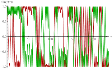
While the non-integrability of a system does not imply chaos necessarily, chaotic dynamics is indicative of the absence of integrability. In this and the next section we will perform numerical analysis of the equations of motion for the extended string we have considered and allow the system to evolve in time. This time evolution reveals chaotic dynamics.

The equations of motion for $x(\tau)$ and $\theta(\tau)$ are coupled in general as we saw, and though we are not able to find exact analytic solutions we can solve them numerically.

We choose to study the $L^{1,7,5}$ manifold. We can immediately see that we get $d=3$ using eq. 8. We have the freedom to set any of the $\alpha,\beta,\mu$ constants to any non-zero value and we choose to set $\mu=1$. We solve the system of equations described by the first equation in eq. 4 as well as the relations described in eq. 11 to determine the values of $\alpha,\beta,x_{1},x_{2},x_{3}$. We obtain $\alpha=2.854,\beta=3.188,x_{1}=0.1192,x_{2}=2.347,x_{3}=3.575$. We can also determine the period of the coordinate $\zeta$, which is equal to $\breve{\zeta}=0.9782$. We solve both of the equations of motion, eqs. 26c and 26d, numerically by choosing as initial conditions $\theta=0.8$ and $x=0.3$. For the winding of the string along the two $U(1)$ angles inside the $L^{1,7,5}$ manifold we choose $\alpha_{1}=1$ and $\alpha_{2}=2$. The initial choice for $x(\tau)$ is such that it lies between the two smallest roots of the cubic equation $\Delta_{x}=0$ as required. We let the system evolve in time and we plot $\sin\theta$ in a similar manner to the $AdS_{5}\times T^{1,1}$ case Basu and Pando Zayas (2011a). The result is presented in Figure 1.

An interesting special case of the $L^{a,b,c}$ models is to consider $b=c$ Benvenuti and Kruczenski (2006); Franco et al. (2006) with the usual condition $a\leq b$. This special class of models has been dubbed generalized conifolds. The $L^{a,b,b}$ case is equivalent to the $L^{a,b,a}$ under some trivial reorderings as is explained in Franco et al. (2006).

We study the generalized conifold given by $L^{1,5,5}$. Following the same steps as before for the $L^{1,7,5}$ we obtain that $d=1$ and we set again $\mu=1$. The values that characterize the model for the constants $\alpha,\beta$ are $1.931,3.315$ respectively. The three roots of the cubic $\Delta_{x}=0$ are given by $x_{1}=0.81825,x_{2}=1.566,x_{3}=3.498$. The coordinate $\zeta$ ranges from $0$ to $\breve{\zeta}=1.501$ and the remaining needed values for the numerical solution of the equations of motion are the same as in the $L^{1,7,5}$ example. As we did previously, we show the time evolution of the string motion in Figure 1.

In both cases, the string motion exhibits chaos.

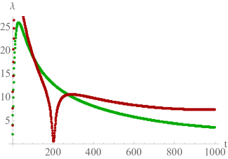
III.1.3 The Lyapunov exponent

A characteristic feature of chaos is the sensitivity of a system to a specific choice for initial conditions. Having said that, we discuss the largest Lyapunov exponent (LLE). The sensitivity on the initial conditions can be phrased in the following way: we can consider any point in the phase space of the theory which we call $X$. There exists at least one point which lies in an infinitesimally close distance to that point and that diverges from it. The said distance is denoted by $\Delta X(X_{0},\tau)$ and is a function of the initial position. The largest Lyapunov exponent is a characteristic quantity that quantifies the rate of separation of such closely laying trajectories in the theory’s phase space. It is given by

$$\lambda=\lim_{\tau\rightarrow\infty}\lim_{\Delta X\rightarrow 0}\left(\frac{1}{\tau}\log\frac{\Delta X(X_{0},\tau)}{\Delta X(X_{0},0)}\right)\,.$$ (41)

We compute the LLE for the systems under consideration. We expect that as we dynamically evolve the system in time and for a chaotic motion, $\lambda$ will converge to some non-zero positive value and fluctuate around that particular value. We have verified that such is the case for the extended string given by eq. 23 that is moving in the $L^{a,b,c}$ manifolds and the result of the computation is shown in Figure 2.

Figure 2: The Lyapunov index for the extended string motion in the $L^{1,7,5}$ manifold (red) with $x(0)=0.12,\theta(0)=\pi/4$ and the $L^{1,5,5}$ model (green) with $x(0)=0.2,\theta(0)=0.1$. For the former, we observe a convergence with $\lambda\approx 7.3$ and for the latter $\lambda\approx 3.5$.

IV BPS mesons and point-like strings

In Benvenuti and Kruczenski (2006) the authors identified the angle conjugate to the R-symmetry and argued that the BPS geodesics resulting from these point-like string modes are compared to the BPS mesons of the quiver theory. Below we study the (non)-integrability of point-like strings.

IV.1 Point-like string motion

We have examined the dynamics of extended string configurations so far. Now we turn our attention to the point-like limit of the string. This limit is obtained very straightforwardly. The change, compared to the previous case, is that the string now is not wrapping the two coordinates inside the $L^{a,b,c}$; simply put we set $\alpha_{1}=\alpha_{2}=0$ in eq. 23.

The Lagrangian can be obtained readily by the previous expression. It is given by:

$$\mathcal{L}=\dot{t}^{2}-\dot{\zeta}^{2}-\frac{\rho^{2}}{4}\left(\frac{\dot{x}^{2}}{\Delta_{x}}+4\frac{\dot{\theta}^{2}}{\Delta_{\theta}}\right)$$ (42)

The equations of motion that follow from the Lagrangian are:

$$\frac{2(\Delta_{\theta}-x)\ddot{x}}{\Delta_{x}}=-\frac{\dot{x}^{2}}{\Delta_{x}}-\frac{4\dot{\theta}^{2}}{\Delta_{\theta}}$$ (43a)

$$+\frac{(\Delta_{\theta}-x)(\alpha\beta-2(\alpha+\beta)x+3x^{2})\dot{x}^{2}}{\Delta^{2}_{x}}$$

$$+2\frac{\dot{x}+(\alpha-\beta)\sin(2\theta)\dot{\theta}}{\Delta_{x}}\dot{x}$$

$$\frac{2(\Delta_{\theta}-x)\ddot{\theta}}{\Delta_{\theta}}=\frac{2\dot{x}\dot{\theta}}{\Delta_{\theta}}-(\alpha-\beta)\sin(2\theta)\left(\frac{\dot{\theta}^{2}}{\Delta_{\theta}}\right.$$ (43b)

$$\left.+\frac{\dot{x}^{2}}{4\Delta_{x}}-\frac{2\dot{\theta}^{2}}{\Delta_{\theta}}+\frac{1}{2\Delta^{2}_{\theta}}(\alpha+\beta\right.$$

$$\left.+(\alpha-\beta)\cos(2\theta)-2x)\dot{\theta}^{2}\right)$$

The Virasoro conditions that constrain the equations of motion for the point-like string read

$$2T_{\tau\tau}=2T_{\sigma\sigma}=-\dot{t}^{2} +\dot{\zeta}^{2}$$ (44a)

$$+\frac{\rho^{2}}{4}\left(\frac{\dot{x}^{2}}{\Delta_{x}}+4\frac{\dot{\theta}^{2}}{\Delta_{\theta}}\right)=0,$$

$$T_{\tau\sigma}=T_{\sigma\tau}=0.$$ (44b)

We can, of course, express the system in a Hamiltonian formalism. The canonical conjugate momenta are given by

$$p_{t} =2\dot{t},\quad p_{\zeta} =-2\dot{\zeta},$$ (45)

$$p_{x} =-\frac{\rho^{2}}{2\Delta_{x}}\dot{x},\quad p_{\theta} =-\frac{2\rho^{2}}{\Delta_{\theta}}\dot{\theta},$$

and the associated Hamiltonian density is equal to

$$\mathcal{H}=\frac{1}{4\rho^{2}}\left[\rho^{2}(p^{2}_{t}-p^{2}_{\zeta})-4\Delta_{x}p^{2}_{x}-\Delta_{\theta}p^{2}_{\theta}\vphantom{\frac{1}{2}}\right]\,.$$ (46)

The invariant plane of solutions on which the equations of motion are satisfied is given by:

$$\{x=x_{0},\dot{x}=\ddot{x}=0,\theta=\theta_{0},\dot{\theta}=\ddot{\theta}=0\}\,,$$ (47)

alongside with the simple solutions

$$t=E~{}\tau+c_{1},\quad\zeta=J~{}\tau+c_{2}\,.$$ (48)

It is quite straightforward to see that if we expand $t=E~{}\tau+c_{1}+\varepsilon\tilde{t}$ as well as $\zeta=J~{}\tau+c_{1}+\varepsilon\tilde{\zeta}$, with $\varepsilon\rightarrow 0$, we are led to the NVEs for the $t$ and $\zeta$ respectively. Both of them admit Liouville integrable solutions.

We can also fluctuate the $x$-coordinate on the invariant plane as $x=x_{0}+\varepsilon\mathcal{X}$ with $\varepsilon\rightarrow 0$ to obtain

$$\frac{(\alpha-\beta)\cos(2\theta_{0})+\alpha+\beta-2x_{0}}{x_{0}(x_{0}-\alpha)(x_{0}-\beta)-\mu}\ddot{\mathcal{X}}=0$$ (49)

which also has Liouville integrable solutions.

Similarly, we can obtain the NVE for the $\theta$-coordinate. We expand as $\theta=\theta_{0}+\varepsilon\vartheta$ in the limit $\varepsilon\rightarrow 0$ and derive

$$\frac{2\left(\alpha\cos^{2}(\theta_{0})+\beta\sin^{2}(\theta_{0})-x\right)}{\alpha\cos^{2}(\theta_{0})+\beta\sin^{2}(\theta_{0})}\ddot{\vartheta}=0$$ (50)

which has Liouville integrable solutions as in the previous cases.

IV.2 Changing coordinates and the R-symmetry angle

Let us briefly describe the change of variables that was introduced in Benvenuti and Kruczenski (2006). It is given by $y=\cos(2\theta)$. Moreover, the said change of variables makes the comparison between BPS geodesics and mesons straightfroward. In order to be able to make a statement for the operators of the boundary quiver, one needs to know the angle conjugate to the R-symmetry. This was also obtained in the aforementioned paper and it reads:

$$\Omega_{R}=3\zeta+\phi+\psi\,,$$ (51)

Now one is able to re-express the geometry eqs. 2 and 3 in terms of this angle and the coordinate $y$. Here we choose not to do that, however we find it useful and illuminating to have this expression explicitly in order to be able to draw conclusions directly using our coordinate system - $\phi,\psi$.

IV.3 BPS mesons from strings

It has been shown that BPS mesons correspond to the BPS geodesics Benvenuti and Kruczenski (2006). These geodesics are such that $x=x_{0}$ and $y=y_{0}$. This can be easily translated into the following statement in our coordinates $x=x_{0}$ and $\theta=\theta_{0}$, where the constants are such that they respect the ranges we have discussed. Moreover, it was argued that the necessary minimization of the Hamiltonian is achieved for $\dot{\phi}=\dot{\psi}=0$. This is the same string configuration that we examined above by taking the point-like limit of the string.

V Epilogue

In this work we considered the motion of an extended string that is localized at the centre of the $AdS_{5}$ space and is wrapping two $U(1)$ angles inside the $L^{a,b,c}$ space. We showed that the dynamics of that particular string configuration is non-integrable, since the Kovacic algorithm fails to provide a solution to the fluctuation equations. We also studied the coupled equations of motion that were derived from the Lagrangian and solved them numerically. The time evolution indicates chaotic dynamics for the string which is another characteristic signature of non-integrability. Having observed the chaotic dynamics, we computed the largest Lyapunov exponent which was found to converge to some positive value.

Since type IIB string theory in the AdS${}_{5}\times L^{a,b,c}$ vacuum is holographically dual to the $\mathcal{N}=1$ quiver gauge theories and we managed to argue that the string picture in the bulk has a translation to the field theory operators, we have, essentially, argued that these particular quiver gauge theories are non-integrable on general grounds.

We also examined the dynamics of a string configuration in the point-like limit and we managed to derive Liouville integrable solutions to the NVE. This is another situation where the integrability of the extended string motion appears to be a much more stringent statement than the integrability of moving particles.

Finally, our work here combined with the results obtained previously in Basu and Pando Zayas (2011a, b) suggest that the classical string motion in the $AdS_{5}\times\mathcal{M}^{5}$ vacuum, with $\mathcal{M}^{5}$ being a five-dimensional Sasaki-Einstein manifold, is non-integrable.

References

- Maldacena (1999) J. M. Maldacena, Int. J. Theor. Phys. 38, 1113 (1999), arXiv:hep-th/9711200 .
- Witten (1998) E. Witten, Adv. Theor. Math. Phys. 2, 253 (1998), arXiv:hep-th/9802150 .
- Gubser et al. (1998) S. Gubser, I. R. Klebanov, and A. M. Polyakov, Phys. Lett. B 428, 105 (1998), arXiv:hep-th/9802109 .
- Sparks (2011) J. Sparks, Surveys Diff. Geom. 16, 265 (2011), arXiv:1004.2461 [math.DG] .
- Gubser (1999) S. S. Gubser, Phys. Rev. D 59, 025006 (1999), arXiv:hep-th/9807164 .
- Klebanov and Witten (1998) I. R. Klebanov and E. Witten, Nucl. Phys. B 536, 199 (1998), arXiv:hep-th/9807080 .
- Gauntlett et al. (2004) J. P. Gauntlett, D. Martelli, J. Sparks, and D. Waldram, Adv. Theor. Math. Phys. 8, 711 (2004), arXiv:hep-th/0403002 .
- Cvetic et al. (2005) M. Cvetic, H. Lu, D. N. Page, and C. Pope, Phys. Rev. Lett. 95, 071101 (2005), arXiv:hep-th/0504225 .
- Martelli and Sparks (2005) D. Martelli and J. Sparks, Phys. Lett. B 621, 208 (2005), arXiv:hep-th/0505027 .
- Martelli and Sparks (2006) D. Martelli and J. Sparks, Commun. Math. Phys. 262, 51 (2006), arXiv:hep-th/0411238 .
- Benvenuti and Kruczenski (2006) S. Benvenuti and M. Kruczenski, JHEP 04, 033 (2006), arXiv:hep-th/0505206 .
- Butti et al. (2005) A. Butti, D. Forcella, and A. Zaffaroni, JHEP 09, 018 (2005), arXiv:hep-th/0505220 .
- Franco et al. (2006) S. Franco, A. Hanany, D. Martelli, J. Sparks, D. Vegh, and B. Wecht, JHEP 01, 128 (2006), arXiv:hep-th/0505211 .
- Beisert et al. (2012) N. Beisert et al., Lett. Math. Phys. 99, 3 (2012), arXiv:1012.3982 [hep-th] .
- Bena et al. (2004) I. Bena, J. Polchinski, and R. Roiban, Phys. Rev. D 69, 046002 (2004), arXiv:hep-th/0305116 .
- Lunin and Maldacena (2005) O. Lunin and J. M. Maldacena, JHEP 05, 033 (2005), arXiv:hep-th/0502086 .
- Frolov (2005) S. Frolov, JHEP 05, 069 (2005), arXiv:hep-th/0503201 .
- Frolov et al. (2005) S. Frolov, R. Roiban, and A. A. Tseytlin, JHEP 07, 045 (2005), arXiv:hep-th/0503192 .
- Berenstein and Cherkis (2004) D. Berenstein and S. A. Cherkis, Nucl. Phys. B 702, 49 (2004), arXiv:hep-th/0405215 .
- Giataganas et al. (2014) D. Giataganas, L. A. Pando Zayas, and K. Zoubos, JHEP 01, 129 (2014), arXiv:1311.3241 [hep-th] .
- Wulff (2017a) L. Wulff, Phys. Rev. D 96, 101901 (2017a), arXiv:1708.09673 [hep-th] .
- Wulff (2018) L. Wulff, JHEP 02, 106 (2018), arXiv:1711.00296 [hep-th] .
- Wulff (2017b) L. Wulff, J. Phys. A 50, 23LT01 (2017b), arXiv:1702.08788 [hep-th] .
- Wulff (2019) L. Wulff, JHEP 04, 133 (2019), arXiv:1903.08660 [hep-th] .
- Pando Zayas and Terrero-Escalante (2010) L. A. Pando Zayas and C. A. Terrero-Escalante, JHEP 09, 094 (2010), arXiv:1007.0277 [hep-th] .
- Giataganas (2019) D. Giataganas, (2019), arXiv:1909.02577 [hep-th] .
- Basu and Pando Zayas (2011a) P. Basu and L. A. Pando Zayas, Phys. Lett. B 700, 243 (2011a), arXiv:1103.4107 [hep-th] .
- Basu and Pando Zayas (2011b) P. Basu and L. A. Pando Zayas, Phys. Rev. D 84, 046006 (2011b), arXiv:1105.2540 [hep-th] .
- Stepanchuk and Tseytlin (2013) A. Stepanchuk and A. Tseytlin, J. Phys. A 46, 125401 (2013), arXiv:1211.3727 [hep-th] .
- Nunez et al. (2018) C. Nunez, D. Roychowdhury, and D. C. Thompson, JHEP 07, 044 (2018), arXiv:1804.08621 [hep-th] .
- Núñez et al. (2018) C. Núñez, J. M. Penín, D. Roychowdhury, and J. Van Gorsel, JHEP 06, 078 (2018), arXiv:1802.04269 [hep-th] .
- Filippas (2020a) K. Filippas, JHEP 02, 027 (2020a), arXiv:1910.12981 [hep-th] .
- Filippas (2020b) K. Filippas, Phys. Rev. D 101, 046025 (2020b), arXiv:1912.03791 [hep-th] .
- Filippas et al. (2019) K. Filippas, C. Núñez, and J. Van Gorsel, JHEP 06, 069 (2019), arXiv:1901.08598 [hep-th] .
- Giataganas and Zoubos (2017) D. Giataganas and K. Zoubos, JHEP 10, 042 (2017), arXiv:1707.04033 [hep-th] .
- Chervonyi and Lunin (2014) Y. Chervonyi and O. Lunin, JHEP 02, 061 (2014), arXiv:1311.1521 [hep-th] .
- Roychowdhury (2017) D. Roychowdhury, JHEP 10, 056 (2017), arXiv:1707.07172 [hep-th] .
- Giataganas and Sfetsos (2014) D. Giataganas and K. Sfetsos, JHEP 06, 018 (2014), arXiv:1403.2703 [hep-th] .
- Roychowdhury (2019) D. Roychowdhury, JHEP 09, 002 (2019), arXiv:1907.00584 [hep-th] .
- Banerjee and Bhattacharyya (2018) A. Banerjee and A. Bhattacharyya, JHEP 11, 124 (2018), arXiv:1806.10924 [hep-th] .
- Kovacic (1986) J. J. Kovacic, Journal of Symbolic Computation 2, 3 (1986).
- Mansson (2007) T. Mansson, JHEP 06, 010 (2007), arXiv:hep-th/0703150 .
- Puletti and Mansson (2012) V. G. M. Puletti and T. Mansson, JHEP 01, 129 (2012), arXiv:1106.1116 [hep-th] .
- Giataganas (2009) D. Giataganas, JHEP 10, 087 (2009), arXiv:0904.3125 [hep-th] .
- Canoura et al. (2006) F. Canoura, J. D. Edelstein, and A. V. Ramallo, JHEP 09, 038 (2006), arXiv:hep-th/0605260 .