Single-shot error correction of three-dimensional homological product codes
Abstract
Single-shot error correction corrects data noise using only a single round of noisy measurements on the data qubits, removing the need for intensive measurement repetition. We introduce a general concept of confinement for quantum codes, which roughly stipulates qubit errors cannot grow without triggering more measurement syndromes. We prove confinement is sufficient for single-shot decoding of adversarial errors and linear confinement is sufficient for single-shot decoding of local stochastic errors. Further to this, we prove that all three-dimensional homological product codes exhibit confinement in their -components and are therefore single-shot for adversarial phase-flip noise. For local stochastic phase-flip noise, we numerically explore these codes and again find evidence of single-shot protection. Our Monte Carlo simulations indicate sustainable thresholds of and for 3D surface and toric codes respectively, the highest observed single-shot thresholds to date. To demonstrate single-shot error correction beyond the class of topological codes, we also run simulations on a randomly constructed 3D homological product code.
I Introduction
Quantum error correction encodes logical quantum information into a codespace roffe2019quantum . Given perfect measurement of the codespace stabilisers we obtain the syndrome of any error present. A suitable decoding algorithm can determine a recovery operation that returns the system to the codespace. Either this recovery is a perfect success, or a failure resulting in a high weight logical error. However, in real quantum systems the measurements are not perfect and this simple story becomes more involved. The three main strategies for tackling noisy measurements are: repeated measurements on the code dennis02 ; FowlerRepMeasure ; performing measurement driven error-correction on a cluster state Raussendorf2007 ; bolt2016foliated ; nickerson2018measurement ; bombin20182d ; brown2019fault ; newman2019generating ; or using a single-shot code and decoder bombin2015single . Focusing on the last strategy, the single-shot approach has the advantage of no additional time cost or cluster-state generation cost and provides a resilience against time-correlated noise bombin2016resilience . In single-shot error correction, some residual error persists after each round of error correction, but this residual error is kept small and does not rapidly accumulate. However, only a special class of codes support single-shot error correction, but exactly which codes and why is not yet fully understood.
Bombín coined the phrase single-shot error correction and remarked that it “is related to self-correction and confinement phenomena in the corresponding quantum Hamiltonian model.” bombin2015single . He defined confinement for subsystem codes, and showed that it is sufficient for single-shot error correction with a limited class of subsystem codes. In particular, he proved that the 3D gauge color code supports single-shot error correction, though it is unknown whether the corresponding Hamiltonian exhibits self-correction. Later single-shot error correction was numerically observed in a variety of higher dimensional topological codes, including: the 3D gauge color code brown15 , 4D surface codes duivenvoorden2018renormalization and their hyperbolic cousins breuckmann2020single , and 3D surface codes with phase noise Kubica2018a ; Kubica2019 ; vasmer2020cellular . Campbell established a general set of sufficient conditions, encapsulated by a code property called good soundness, that ensured adversarial noise campbell2019theory could be suppressed using a single-shot decoder. While Campbell’s sufficiency conditions explained single-shot error correction in a wide range of codes, around the same time it was shown that quantum expander codes tillich2014quantum ; leverrier15 ; fawzi2018 supported single-shot error correction leverrier18 . However, quantum expander codes lack the soundness property so neither Bombín’s notion of confinement or Campbell’s notion of soundness is sufficient to encompass all known examples of single-shot error correction.
We can use different classical algorithms to decode a given quantum code, and this choice will affect the utility of the code. Different decoders have various time complexities and error tolerances, which affects the resources required by a quantum computer based on the code fowler12b ; terhal2015review ; Das2020 . Thus far, single-shot decoders come in two flavours. The first are two-stage decoders brown15 ; duivenvoorden2018renormalization , where: stage 1 decoding repairs the noisy syndrome using redundancy in the parity check measurements; stage 2 decoding solves the corrected syndrome problem. The second flavour of decoders compute a correction from the noisy syndrome without attempting to repair it. Most examples of such decoders are local decoders, meaning that the whole correction is made up of corrections computed in small local regions of the code using syndrome information in the immediate neighbourhood Kubica2018a ; Kubica2019 ; vasmer2020cellular ; fawzi2018 ; grospellier2018numerical ; grospellier2020combining ; breuckmann2020single . However, there are some examples of non-local decoders such as belief propagation (BP) being used for single-shot error correction without syndrome repair breuckmann2020single ; grospellier2020combining . A natural question to ask is: what is the optimal decoding strategy for single-shot codes? Even in the simple case of the 3D toric code this is not well-understood.
The remainder of this article is structured as follows. In Sec. II, we give a summary of our results. In Sec. III, we formally state our results on confinement and single-shot decoding. In Sec. IV, we detail the construction of 3D product codes. In Sec. V, we present our numerical simulations and analyse their results. Finally, in Sec. VI, we discuss future research directions that flow from this work.
II Summary of results
This article is in two parts: on the one hand, we propose the concept of confinement as an essential characteristic for a code family to display single-shot properties; on the other, we investigate the single-shot performances of the class of 3D homological product codes tillich2014quantum ; bravyi14 ; audoux2015tensor , which we call 3D product codes. We introduce confinement in Sec. III. Loosely, confinement stipulates that low-weight qubit errors will result in low-weight syndromes. We then formalise the notion of a code family having good confinement, which we prove is a sufficient condition for single-shot decoding in the adversarial noise setting. In addition to that, we prove that good linear confinement is a sufficient condition for a family of codes to exhibit a sustainable single-shot threshold for local stochastic noise (App. A). We review the construction of the 3D product codes in App. IV, and show that the 3D surface and toric codes are particular instances of this more general class of codes in Sec. B. We prove that all 3D product codes have (cubic) confinement for phase-flip errors (App. C), and therefore have single-shot error correction for adversarial phase-flip noise. We expect these codes to have single-shot error correction for local stochastic phase-flip noise as well. In fact, our definition of confinement generalises the definition proposed by Bombín bombin2015single for the gauge color code and the notion of robustness for expander codes leverrier15 ; since both class of codes are proven to have a single-shot threshold for local stochastic noise bombin2015single ; leverrier18 we conjecture that low density parity check (LDPC) codes with good (super linear) confinement have a threshold too. We investigate this case numerically.
In the single-shot setting, the code always has some residual error present and the error correction procedure introduces noise correlations in subsequent rounds of single-shot error correction. How then do we assess success or failure of a decoding algorithm? The concept of the sustainable threshold was proposed by Brown, Nickerson and Browne brown15 as a metric for single-shot codes and decoders. We use to denote the threshold of a code-decoder family given cycles of qubit noise, noisy syndrome extraction and single-shot decoding, with the cycle followed by a single round of noiseless syndrome extraction and decoding. The final round ensures that we can return the system to the codespace and assess success by the absence of a logical error. We define the sustainable threshold of the code-decoder family to be
| (1) |
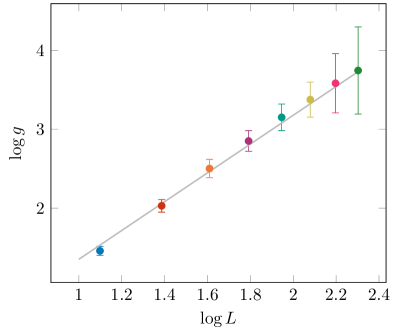
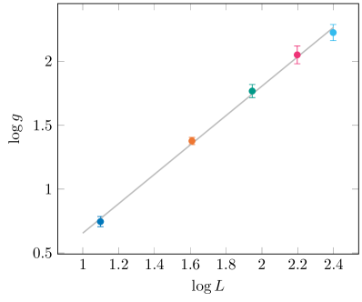
Numerically, this is estimated by plotting against and fitting to the following ansatz,
| (2) |
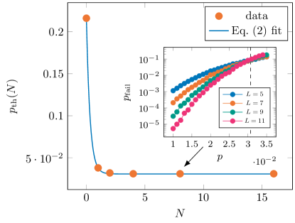
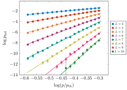
We numerically estimate the sustainable error thresholds of 3D toric and surface codes for two different two-stage decoders. We surpass all previous single-shot error thresholds for these code families, and we also obtain the highest code-capacity noise (no measurement error) threshold; see Table 1. For our single-shot simulations, we use an independent and identically distributed (iid) noise model where each qubit experiences a phase-flip error with probability , and each stabiliser measurement outcome is flipped with probability . We investigate two decoding strategies: one where we use minimum-weight perfect matching (MWPM) for stage 1 decoding and belief propagation with ordered statistics decoding (BP+OSD) for stage 2 decoding and another where we use BP+OSD for both decoding stages. Fig. 1 shows the 3D surface code sustainable threshold fit, using the MWPM & BP+OSD decoding strategy. We find a comparable sustainable threshold for the 3D surface code using BP+OSD for both decoding stages, as shown in Table 2. We achieve very similar performance for the 3D toric code, although there is a subtlety present in stage 1 decoding that is not present in the 3D surface code case; see Sec. V.3. For both code families, we provide evidence that the performance of stage 1 decoding is the bottleneck of the full decoding procedure, and we achieve near-optimal performance within this constraint.
| Decoder | ||
|---|---|---|
| Erasure Mapping Aloshious2019 | N/A | |
| Toom’s Rule Kubica2018a | N/A | |
| Sweep* vasmer2020cellular | ||
| Renormalization Group duivenvoorden2018renormalization | 7.3(1)% | |
| Neural Network Breuckmann2018 | 17.5% | 7.1(3)% |
| MWPM + BP/OSD* | ||
| Optimal Ozeki1998 ; Ohno2004 ; Hasenbusch2007 ; takeda2004 ; Kubica2018 | 23.180(4)% | 11.0% |
| Code | MWPM & BP+OSD | BP+OSD x2 |
|---|---|---|
| Surface | 3.08(4)% | 2.90(1)% |
| Toric | 2.90(2)% | 2.78(2)% |
The advantage of using BP+OSD for stage 1 decoding is that, unlike MWPM, this decoder does not rely on the special structure of the loop-like syndrome present in 3D toric and surface codes. Therefore, we anticipate that one can use BP+OSD for single-shot decoding of general 3D product codes. We numerically test this prediction by decoding a family of non-topological 3D product codes using BP+OSD for both decoding stages, achieving sustainable thresholds that are comparable to those of the 3D toric and surface codes. This provides evidence that BP+OSD can be used as a generic two-stage decoder for single-shot LDPC 3D product codes.
III Formal statements
In this Section we introduce the definition of confinement for a stabiliser code and exhibit a theoretical two-stage decoder, the Shadow decoder, which we prove is single-shot on confined codes against adversarial noise. We refer the reader to App. A to see how a variant of the Shadow decoder can be used to prove that good families of codes with linear confinement have a single-shot threshold for local stochastic noise.
A stabiliser code encoding logical qubits into physical qubits can be described by its stabiliser group and a syndrome map . The stabiliser group is an Abelian subgroup of the Pauli group on qubits which does not contain and has dimension . The syndrome map is not unique: any generating set of the group defines a valid syndrome map for the code. If is one of such generating sets, the associate function maps a qubit operator into the binary vector , where if anti-commutes with and otherwise. Importantly, is linear, meaning that over . Because any Pauli operator can be factorised as the product of an and a -operator and , we can identify it with a binary vector , where the th entry of is if and only if acts non-trivially on the th qubit. Given a Pauli operator , its weight is the number of qubits on which its action is not the identity. Fixed a stabiliser code with syndrome function , the reduced weight of a Pauli operator on the physical qubits is
A stabiliser code is said to be distance if is the minimum weight of a Pauli operator not in that has trivial syndrome. We will refer to a code of length , dimension and distance as a code.
For a stabiliser code, we then have
Definition 1 (Confinement).
Let be an integer and some increasing function with . We say that a stabiliser code has -confinement if, for all errors with , it holds
Let us contrast this with Bombín’s notion of confinement (Def. 16 of Ref. bombin2015single ) that has some similarities but only allows for linear functions of the form for some constant . Many codes, including 3D product codes, have superlinear confinement functions, as such Bombín’s definition does not encompass them. Moreover, the concept of confinement is closely related to soundness campbell2019theory but it is weaker and so able to encompass more families of codes, such as the expander codes tillich2014quantum ; leverrier15 ; fawzi2018 which are confined but not sound. Roughly speaking, a code has good confinement if small qubit errors produce small measurement syndromes; this differs from good soundness which entails that small syndromes can be produced by small errors.
Formally, we define the following notion of good confinement for a family of stabiliser codes
Definition 2 (Good confinement).
Consider an infinite family of stabiliser codes. We say that the family has good confinement if each code in it has -confinement where:
-
1.
grows with the length of the code: with ;
-
2.
and is monotonically increasing and independent of .
We say the code family has good -confinement if the above holds only for Pauli- errors.
Our main analytic result is that codes with good confinement are single-shot
Theorem 1.
Consider a family of quantum-LDPC codes with good confinement such that with and . This code family is single-shot for the adversarial noise model. If the code family only has good -confinement then it is single-shot with respect to Pauli- noise.
We conjecture that the result of Thm. 1 can be extended to deal with local stochastic noise and used to show that LDPC codes with good confinement have a single-shot threshold. In this direction, we are able to prove that linear confinement is sufficient for codes to exhibit a single-shot threshold in the local stochastic noise setting:
Theorem 2.
Consider a family of quantum-LDPC codes with qubit degree at most and good linear confinement such that with and . This code family has a sustainable single-shot threshold for any local stochastic noise model. If the code family only has good -confinement then it has a sustainable single-shot threshold with respect to Pauli- noise.
We further prove that 3D product codes have -confinement:
Theorem 3.
All 3D product codes have -confinement where is equal to the -distance of the code and or better.
We now proceed to prove Thm. 1. To this end, we use the Shadow decoder that we introduce in Def. 3. The Shadow decoder differs from previous single-shot two stage decoders (e.g. the MW single-shot decoder introduced in Def. 6 of campbell2019theory ) in that it does not rely on metachecks on syndromes. If syndromes are protected by a classical code, as it is the case for -syndromes of 3D product codes introduced in Sec. IV, then a single-shot decoding strategy could work as follows: (1) correct the measured syndrome whenever it does not satisfy all the constraints defined by the metacode; (2) find a recovery operator on qubits that has syndrome equal to the one found at point (1). The Shadow decoder, instead, corrects the syndrome both anytime it fails to satisfy all the constraints of the metacode and when it is generated by high weight errors. We do not describe how to implement it or make statements concerning the complexity of decoding. Our proof makes similar assumptions as the Kovalev-Pryadko quantum-LDPC threshold theorem Kovalevbadcode where they assumed a minimum weight decoder without addressing implementation issues. Indeed, decoding for arbitrary LDPC codes is an NP-complete problem that we do not expect to be efficiently solvable in full generality.
The building blocks of the Shadow decoder are the s of the code. A is a set in the syndrome space which contains all the images of Pauli errors on the physical qubits that have weight at most . In other words, if we identify Pauli errors on qubits with -bit strings and we consider the metric space endowed with the Hamming distance (i.e. the distance between the vectors and corresponding to the Pauli errors and respectively is defined as ) then the of the code is the image, via the syndrome function , of the ball of radius centered at in . Note that, because balls on are not vector spaces, the are not vector spaces either.
We are now ready to introduce the Shadow decoder.
Definition 3 (Shadow decoder).
The Shadow decoder has variable parameter . Given an observed syndrome where is the syndrome error, the Shadow decoder of parameter performs the following 2 steps:
-
1.
Syndrome repair: find a binary vector of minimum weight such that belongs to the of the code, where
-
2.
Qubit decode: find of minimum weight such that .
We call the residual error.
A key result in proving Thm. 1 is the following promise on the performance of the Shadow decoder: when a code has confinement, the weight of the residual error after one decoding cycle is bounded by a function of the weight of the syndrome error.
Lemma 1.
Consider a stabiliser code that has -confinement. Provided that the original error pattern has , on input of the observed syndrome , the residual error left by the Shadow decoder of parameter satisfies:
| (3) |
Proof.
Assume . By construction, has minimum weight among all errors with syndrome of the code. In particular . By the triangular inequality for the weight function,
| (4) |
Therefore, we can apply the confinement property on the residual error :
| (5) |
By linearity of the syndrome function :
| (6) |
Note that the syndrome error is a possible solution of the syndrome repair step of the Shadow decoder, because by assumption . Thus, and
| (7) |
Combining these and the monotonicity of leads to the required bound on the residual error:
| (8) |
∎
Thm. 1 follows directly from Lem. 1. In particular, Lem. 1 entails that a code with -confinement is robust against cycles of qubit noise, noisy syndrome extraction and single-shot decoding, as explained below.
At each cycle , we assume that a new error is introduced in the system and it is added to the residual error . We assume that for the new physical error and the syndrome measurement error the following hold:
| (9) |
We perform syndrome extraction on the state . The noisy syndrome is used as input for the Shadow decoder of parameter . The recovery operator found by the Shadow decoder is then applied to the state and finally a new cycle starts where . Let , so that the initial state of the system is given by , . Note that if
| (10) |
then and the hypotheses of Lem. 1 hold. Combining this with the bound on the syndrome error (9), we obtain
In conclusion, provided that the conditions on the physical and the measurement error (9) are satisfied for each iteration up to , the residual error after the cycle is kept under control too.
Thm. 2 is proven in App. A. There, we introduce a novel notion of weight to describe local stochastic errors: the closeness weight. We then present the Stochastic Shadow decoder, a variant of the (Adversarial) Shadow decoder of Def. 3. Importantly, on confined codes, it keeps the the closeness weight of the residual error under control over repeated correction cycles. Finally, the proof of Thm. 2 follows by combining these results with some classic percolation theory bounds.
The proof of Thm. 3 is very technical and is deferred to App. C. It is an adaption of the one of soundness for 4D codes given in campbell2019theory , and it is reported in this manuscript for completeness. We remind the reader that, for our numerical studies on 3D product codes, we do not use the Shadow decoder, but rather heuristics that perform well in practice. In particular, we use a two-stage decoder that exploits a metacheck structure on syndromes and attempts to repair the syndrome if and only if it does not pass all metachecks.
Our main motivation to introduce the concept of confinement and the Shadow decoder was to find a feature of codes able to encompass all known examples of single-shot codes. Campbell campbell2019theory introduced the notion of soundness and showed that this property is a sufficient condition for codes to show single-shot properties in the adversarial setting. Nonetheless, Fawzi et al. leverrier18 showed that expander codes have a single-shot threshold for local stochastic noise, even though they do not have the soundness property. As already said though, expander codes do have confinement. In Corollary 9 of leverrier15 the authors prove that their confinement function is linear and call this property robustness. Confinement, in other words, fills the gap leaved by the concept of soundness. Furthermore, as Lem. 2 states, it is a requirement strictly weaker than soundness: any LDPC family of codes with good soundness has good confinement.
Definition 4 (Soundness campbell2019theory ).
Let be an integer and be a function with . Given a stabiliser code with syndrome map we say it is -sound if for all error sets with it follows that .
Definition 5 (Good soundness campbell2019theory ).
Consider an infinite family of codes with syndrome maps . We say that the family has good soundness if each code in it is -sound where:
-
1.
grows with such that with ;
-
2.
and is monotonically increasing and independent of .
It follows easily from Campbell’s definition of soundness and our definition of confinement that the former entails the latter.
Lemma 2.
Consider a LDPC code that is -sound with increasing. If its qubit degree is at most , then it has -confinement.
Proof.
If is an error set with , for its syndrome the following holds:
| (11) |
By soundness of the code:
| (12) |
∎
In conclusion, confinement does answer to the need of finding general and inclusive properties related to single-shot error correction. The reminder of this article is devoted to the study of the 3D product codes. We recall their construction in Sec. IV and we numerically assess their single-shot performance under local stochastic noise in Sec. V.
IV Code construction
The identification of pauli operators with binary vectors is a group homomorphism (i.e. multiplication of Pauli operators corresponds to the sum of their vector representation in ) and because is linear, syndrome measurement can be simulated via a matrix-vector product:
where the vector represents a Pauli error on the physical qubits. Following the nomenclature from classical coding theory, we refer to the syndrome matrix as parity check matrix and we say that a code is LDPC when its parity check is low density.
A stabiliser code is a CSS code if its stabiliser group can be generated by the disjoint union of a set of -operators and a set of -operators. In this case, its parity check is a block matrix:
| (15) |
where has size and has size if the generating set of -stabilisers/-stabilisers has cardinality /. Eq. (15) entails that syndrome extraction can be performed separately for the -component and for the -component. In fact, if a Pauli operator has vector representation , then for its syndrome holds:
where and . In other words, it is possible to truncate these vectors without loosing information and deal with and operators separately. For this reason, we say that a CSS code is provided with two syndrome maps which correspond to the two blocks/matrices and respectively. Accordingly, a CSS code will have a -distance and a -distance and can be compactly be refereed to as a code.
To our purpose, it is handy to describe CSS codes in terms of chain complexes. A length chain complex is a collection of vector spaces and linear maps with the only constraint
| (16) |
for . If and are and binary matrices as in Eq. (15), then the chain complex:
| (17) |
is well defined. In fact, the commutative condition on the stabilisers of the code entails that the -generators and the -generators of the code have even overlap, such that they are orthogonal when seen as binary vectors. In other words, is equivalent to the defining property of chain complexes (see Eq. (16)). In general, we can associate a CSS code to any chain complex of length at least by equating and for some index . In the chain complex language, we say that the code has length and the dimension of the -th homology group . Equivalently, the dimension of the code is the dimension of the -th cohomology group . The and distances are given respectively by the minimum weight of any non-zero vector in and .
Here, we study some decoding properties of 3D product codes. By this nomenclature we refer to the CSS codes obtained by the homological product of three length-1 chain complexes as described in pryadko2018hp . Given three classical linear codes with parity check matrices and we can build a 3D quantum code as follows. If is a binary matrix of size , it defines a linear map , where , are vector spaces over of dimension and respectively; in other words, each linear map defines a length-1 chain complex. The 3D product of the seed matrices , is the length-3 chain complex given by:
where:
The symbol represents the tensor product. Given two vector spaces and over a field , their tensor product is the vector space generated by the formal sums where and and the operator is bilinear, i.e. for any in and respectively, it holds that
The horizontal stacking of spaces, instead, represents their direct sum.
It is easy to verify that condition (16) is verified for and therefore the chain complex is well defined. As explained above, we define a CSS code on by equating
We refer to the matrix as the metacheck matrix for the -stabilisers. Condition (16) entails and as a consequence we can think of the matrix as a parity check matrix on the syndromes: any valid -syndrome satisfies the constraints defined by .
Let be the parameters of the classical linear code with parity check matrix . As showed in pryadko2018hp , is thus associated with an code such that, if ,
By convention, the the distance of a code with dimension is . We define the single-shot distance campbell2019theory of the chain complex as the minimum weight of a vector in that satisfies all the constraints given by (i.e. it belongs to the kernel of ) but is not a valid -syndrome (i.e. it does not belong to the image of ). In other words, is the minimum weight of a vector in the second homology group of the chain complex . Following pryadko2018hp it is easy to verify that if and otherwise.
It is important to note that, if the matrices are LDPC, then their 3D product code is quantum-LDPC. In fact, if has column (row) of weight bounded by (), then has column and row weight bounded by and respectively where:
-
i.
and
-
ii.
and
; -
iii.
and .
IV.1 On geometric locality
In addition to preserving the LDPC properties of the seed matrices, the 3D product yields local codes when qubits are placed on edges of a 3D cubic lattice. We defer the reader to App. B for a thorough discussion on the embedding of 3D product codes on a cubic lattice and we here present a loose summary.
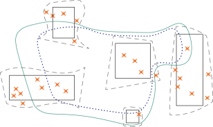
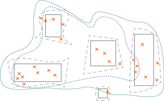
Qubits of a 3D product code associated to the chain complex are in bijection with basis elements of the space ; since is the direct sum of the three vector spaces , and we introduce three different type of qubits: transverse, vertical and horizontal. Qubit types naturally correspond to the three different orientation of edges on a cubic lattice, namely edges parallel to each of the three crystal planes. Referring to this particular display of qubits, the stabilisers of the code defined by have support as follows:
-
1.
-stabilisers have support on a 2D cross of qubits of two types out of three, contained in one of the three crystal planes; the crossing is defined by a square face of a cube (see Fig. 7);
-
2.
-stabilisers have support on a 3D cross of qubits, with crossing defined by a vertex of a cube (see Fig. 8).
The cubic lattice considered can present some irregularities: in general it is a cubic lattice with some missing edges. Nonetheless, square faces and vertices are uniquely defined and they correspond to a stabiliser every time they contain at least one edge. More specifically, a square face identifies two perpendicular lines of edges/qubits on a plane which are the edges parallel to the boundary of the square face itself. The corresponding -stabiliser has support contained on those lines of edges/qubits. Similarly, a vertex identifies three perpendicular lines of qubits and the corresponding -stabiliser has support there contained. When combined with some locality properties of the seed matrices, this characteristic ‘cross shape’ of the stabilisers support entails that 3D product codes are local on a cubic lattice (Prop. 1 in App. B). Here, by locality, we mean that for some positive integer , hold:
-
1.
any -stabiliser generator has weight at most with support contained in a 2D box of size ,
-
2.
any -stabiliser generator has weight at most with support contained in a 3D box of size ,
Interestingly, it follows easily as a corollary of our locality proof that the 3D toric and surface codes are in fact 3D product codes. We now detail an explicit construction of the 3D toric and surface codes as 3D product codes and we remind the reader to App. B for further details.
The 3D toric code is the 3D product code obtained by choosing as seed matrices, where is the parity check matrix of the repetition code. For instance, the 3D toric code with linear lattice size is given by
In general, the 3D toric code of lattice size , has parameters
and single-shot distance .
The 3D surface code is obtained from this construction by choosing, for linear lattice size ,
and
Therefore, for lattice size , it has parameters
and single-shot distance .
Further details can be found in App. B.
IV.2 Non-topological codes
The 3D product code construction can be used to obtain non-topological codes with non-local interactions. Table 3 shows the parameters for a class of non-topological codes based on classical LDPC codes. The specific advantage of non-topological codes is that it is possible to construct code families where the number logical qubits increases with the code length. This is in contrast to 3D toric and surface codes, where the number of logical qubits is fixed for all values of the code distance.
V Numerics
To assess the single-shot performance of the 3D product codes, we simulate the decoding of phase-flip () errors. As 3D product codes are CSS codes, the relevant stabilizers are the -stabilizers. Let describe the support of a phase-flip error, i.e. if qubit has a phase-flip error. The syndrome, , of this error is then
| (18) |
where is the parity check matrix of the -stabilizers of the code (see Eq. (15)).
Owing to the chain-complex structure of 3D product codes (outlined in Sec. IV) the syndromes are themselves the codewords of a classical linear code with parity check matrix such that for all . We refer to such a code on the syndromes as metacode. The metacheck matrix can be used to detect and correct syndrome noise.
In a two-stage single-shot decoder, stage 1 decoding corrects the syndrome noise using before stage 2 decoding corrects the data qubits. In general, decoding is an NP-complete problem that cannot be solved exactly in polynomial-time. However, good heuristic techniques exist that allow approximate solutions to be efficiently computed. In this work, we use two such decoding methods: minimum weight perfect matching (MWPM) and belief propagation plus ordered statistics decoding (BP+OSD). Both MWPM and BP+OSD are algorithms that run over graphical models that encapsulate the structure of the code. We now briefly describe each decoder.
V.1 Minimum weight perfect matching (MWPM)
The minimum weight perfect matching (MWPM) decoder is useful for codes that produce pairs of syndromes at the ends of error chains. The method works by mapping the decoding problem to a graphical model in which nodes represent the code syndromes and weighted edges represent error chains of different lengths. For a given pair of syndrome excitations, the MWPM algorithm deduces the shortest error chain that could have caused it Edmonds1965 .
MWPM finds use for a variety of topological codes, most famously for the 2D surface and toric codes dennis02 ; Fowler12 ; breuckmann2016 ; Brown2020 ; kubica2019efficient . For 3D codes, MWPM is a suitable candidate for syndrome repair step referred to as stage 1 decoding. Specifically, the syndrome of a phase-flip error can be viewed as a collection of closed loops of edges in a simple cubic lattice111Namely, the dual lattice of the one described in App. B. (with boundary conditions depending on the code). Measurement errors cause loops of syndrome to be broken, and the job of stage 1 decoding is to repair these broken syndromes. To obtain the corresponding matching problem, we create a complete graph whose vertices correspond to the break-points of the broken syndrome loops, with edge weights that are equal to the path lengths between the break-points. We use the Blossom V Kolmogorov2009 implementation of Edmonds’s algorithm to solve this matching problem. The edges in the matching correspond to the syndrome recovery operators.
V.2 Belief propagation + ordered statistics decoding (BP+OSD)
Belief propagation (BP) is an algorithm for performing inference on sparse graphs that finds widespread use in high-performance classical coding. Classical LDPC codes, for example, achieve performance close to the Shannon-limit when decoded with BP mackay1997near . In the context of quantum coding, BP is useful for codes that do not produce pairs of syndromes and therefore cannot be decoded with MWPM.
The BP algorithm maps the decoding problem to a bipartite factor graph where the two node species represent data qubits and syndromes respectively. Graph edges are drawn between the data and syndrome nodes according to the code’s parity check matrix. The factor graph is designed to provide a factorisation of the probability distribution that describes the relationship between syndromes and errors. The BP algorithm proceeds by iteratively passing ‘beliefs’ between data and syndrome nodes, at each step updating the probability that a data node is errored. The algorithm terminates once the probability distribution implies a error pattern that satisfies the inputted syndrome.
For quantum codes, the standard BP algorithm alone does not achieve good decoding performance due to the presence of degenerate errors. These cause ‘split-beliefs’ and prevent the algorithm from terminating. Fortunately, the problem of split-beliefs can be resolved by incorporating a post-processing technique known as ordered statistics decoding (OSD). The OSD step uses the probability distribution outputted by BP to select a low-weight recovery operator that satisfies the syndrome equation.
The BP+OSD algorithm was first applied to quantum expander codes by Panteleev and Kalachev panteleev2019degenerate . Following this, Roffe et al. roffe2020decoding demonstrated that the BP+OSD decoder applies more widely across a broad range of quantum-LDPC codes, including the 2D surface and toric codes. For this work, we use the software implementation of BP+OSD from roffe2020decoding , which can be downloaded from bp_osd_github .
V.3 The two-stage single-shot decoding algorithm
Our simulations of the two-stage single shot decoder employ two strategies. (1) MWPM & BP+OSD: stage 1 decoding is performed using MWPM and stage 2 decoding uses BP+OSD. (2) BP+OSD2: both stages are BP+OSD.
Algorithm 1 describes our methodology for the simulations of the two-stage single-shot decoder.
The 3D toric code has a failure mode that is not present in the 3D surface code. In such codes, syndromes exist that satisfy all of the metachecks, , but are invalid syndromes, meaning that does not belong to the image of . In other words, is invalid if there is no error vector with syndrome but it is a codeword of the metacode.
Referring to the chain complex structure of :
we see that these non-valid syndromes are non-trivial elements of the nd homology group:
If is the dimension of , the set of invalid syndromes is a vector subspace of of dimension whose vectors can be written as where is a representative of the equivalence class and . Thus, if is a matrix whose columns are vectors in that generate (meaning that they belong to different equivalence classes in ), we can write any invalid syndrome as:
| (19) |
where is non-zero if and only if is invalid and is any error vector in .
By duality on , the nd cohomolgy group:
has order too. If is a matrix whose rows generates , then the product has full rank because both and have full rank. Moreover, since the rows of in particular belongs to , it holds . Combining these two observations with Eq. (19) yields:
where if and only if because is full rank. In conclusion, we have found that:
if and only if is an invalid syndrome. As a consequence, we can assess whether a syndrome is invalid or not by calculating this product. The meaning of matrices and can be understood by looking at elements in and as logical operators of a CSS code defined on with qubits in (see Sec. IV). In this settings, the full rank condition translates in the anticommuting relation between logical and logical operators of the code.
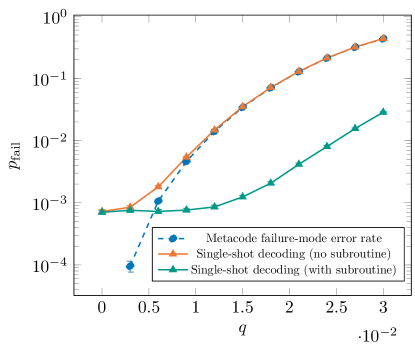
In the 3D toric code, these invalid syndromes are loops of edges around one of the handles of the torus, and are equivalent to the logical operators of the metacode. It is therefore possible to check whether stage 1 decoding results in such a failure by checking whether the repaired syndrome anti-commutes with a matrix whose rows generate the relevant group of the logical operators of the metacode. When a metacode failure is encountered, a failure-mode subroutine (line 15 of Algorithm 1) is called that forces the repaired syndrome into the correct form. This sub-routine involves using BP+OSD to decode a modified version of the metacheck matrix defined as follows
| (20) |
The additional constraints in the modified metacheck matrix ensure that the repaired syndrome is never an invalid syndrome. We call this procedure as a subroutine (rather than all the time) as the component causes to have higher maximum row and column weights than , resulting in a reduction in BP decoding performance. Indeed, the rows of must have weight lower bounded by the transpose distances of the seed codes222More precisely, rows of are vectors in that correspond to elements of the second cohomology group ; hence their weight is lower bounded by , see pryadko2018hp .. Since the transpose distances of the seed codes also determine the -distance of the quantum code (Sec. IV), we want these quantities to be growing with the length of the code and therefore the matrix is not, in general, LDPC.
We find that whilst the failure-mode subroutine does not change the error threshold of the decoder, it does considerably reduce the logical error rate. This is illustrated by Fig. 2, which shows the single-shot logical error rate with and without the failure-mode subroutine. For large syndrome error rates, Fig. 2 shows the failure-mode subroutine improves decoding performance by over an order of magnitude.
V.4 3D toric and surface codes
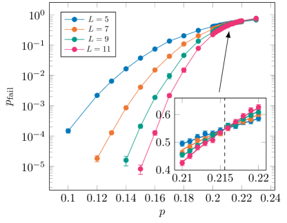
We estimate the sustainable threshold of the 3D toric and surface codes using our two decoding strategies. For code-capacity noise (i.e. perfect syndrome measurements), the syndrome-repair step is not required, so both decoding strategies are the same. For each code family, we observe a code capacity threshold of , as illustrated in Fig. 3. To obtain our threshold estimates, we use the standard critical exponent method Harrington2004 (see App. D for details). In the single-shot setting, we find similar performance for both our decoding strategies, as summarized in Table 2. Our results compare favourably with the performance of other decoders, which we list in Table 1. We obtain the highest reported code-capacity threshold and the highest reported single-shot threshold.
We remark that the sustainable threshold that we observe for the 3D toric code is very close to the threshold of MWPM for string-like errors in the 3D toric code wang03 . This implies that the performance of decoder 1 (the syndrome-repair step) is limiting the performance of the entire decoding procedure, as was suggested in duivenvoorden2018renormalization . Although the sustainable thresholds we observe for 3D surface codes are slightly higher than for 3D toric codes, the codes we consider are relatively small, which means that boundary effects may be having an impact on our sustainable threshold estimates.
We also investigated the suppression of the logical error rate below threshold in the 3D toric code, using MWPM & BP+OSD. We use the following ansatz for the logical error rate for values of ,
| (21) |
where and are parameters to be determined. The code distance of the 3D toric code for errors is , so if the decoder is correcting errors up to this size, we would expect . Using the fitting procedure described in App. D, we estimate for (code capacity) and for (eight rounds of single-shot error correction). Therefore, for the (relatively small) codes that we consider, we find evidence that BP+OSD is correcting errors of weight up to the code distance. Viewed as an error correction problem, the distance of the syndrome-repair step of decoding (i.e the single-shot distance ) is , which is consistent of our observed value of in the single-shot case. This provides further evidence that the bottle-neck of our single-shot decoding procedure is the syndrome-repair step.
V.5 Non-topological codes
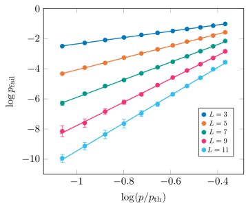
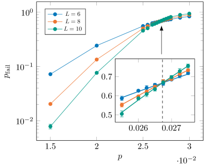
So far, we have focused on the decoding of 3D topological codes. We now show that the BP+OSD decoder can be used for single-shot decoding of more general 3D product codes. Table 3 shows a family 3D product codes constructed by taking the 3D product of a -LDPC code333A code whose parity check matrix has rows/columns of weight 3/4. with two instances of the classical repetition code. The result is a code family where the number of logical qubits is not fixed. This code family was decoded using a two-stage single-shot decoder, BP+OSD , yielding the threshold plot in Fig. 4. The simulation results suggest a sustainable threshold in the region of .
VI Conclusion
In this article, we investigated single-shot decoding of 3D product codes. We gave a formal definition of confinement in quantum codes and proved that all 3D product codes have confinement for errors. We also proved that confinement is sufficient for single-shot error correction against adversarial noise. This is a strengthening of the result of Campbell campbell2019theory , who showed that a property called soundness is sufficient for single-shot error correction, in that soundness implies confinement but the converse is not true. Remarkably, there are important classes of codes, such as quantum expander codes, which have confinement but not soundness. Further to that, we prove that codes with linear confinement, and so expander codes, do have a single-shot threshold for local stochastic noise. The obvious open problem arising from our work is how to extend our findings for linear confinement to the super linear case. Is confinement, in general, a sufficient condition for quantum-LDPC codes to exhibit a single-shot threshold? If not, what other requirements should a code satisfy to ensure the existence of a single-shot threshold?
We simulated single-shot error correction for a variety of 3D product codes, concentrating on 3D toric and surface codes. Using MWPM & BP+OSD, we achieved the best known code capacity error threshold and sustainable single-shot error threshold for this code family (for phase-flip noise). Our results strongly suggest that the bottleneck of two-stage decoders is the first stage where the noisy syndrome is repaired. For the 3D toric code, the optimal threshold of the syndrome repair step is Ohno2004 , whereas the optimal threshold of the entire decoding problem is takeda2004 . This implies that two-stage decoders can never achieve optimal performance in these codes, so perhaps other single-shot decoding methods ought to be investigated in future.
We also simulated single-shot error correction for a family of non-topological 3D product codes, using BP+OSD for both decoding steps. We achieved performance very close to that of the 3D toric and surface codes, which indicates that BP+OSD is a high-performance single-shot decoder. Furthermore, the versatility of BP+OSD means that we expect it to work as a single-shot decoder for general LDPC 3D product codes. We leave confirmation of this to future work, and we conjecture that BP+OSD will achieve good performance for other classes of quantum-LDPC codes such as topological fracton codes Vijay2016 ; Dua2019 .
Acknowledgements.- This work was supported by the Engineering and Physical Sciences Research Council [grant numbers EP/P510270/1 (J.R.S.) and EP/M024261/1 (E.T.C. and J.R.)]. M.V. thanks Aleksander Kubica and Nikolas Breuckmann for illuminating discussions. We thank Rui Chao for comments on an early version of the manuscript. Research at Perimeter Institute is supported in part by the Government of Canada through the Department of Innovation, Science and Economic Development Canada and by the Province of Ontario through the Ministry of Colleges and Universities. This research was enabled in part by support provided by Compute Ontario (www.computeontario.ca) and Compute Canada (www.computecanada.ca). This work was completed while ETC was at the University of Sheffield.
References
- [1] Joschka Roffe. Quantum error correction: an introductory guide. Contemporary Physics, 60(3):226–245, 2019.
- [2] Eric Dennis, Alexei Kitaev, Andrew Landahl, and John Preskill. Topological quantum memory. Journal of Mathematical Physics, 43(9):4452–4505, 2002.
- [3] Austin G. Fowler, Ashley M. Stephens, and Peter Groszkowski. High-threshold universal quantum computation on the surface code. Phys. Rev. A, 80:052312, 2009.
- [4] R Raussendorf, J Harrington, and K Goyal. Topological fault-tolerance in cluster state quantum computation. New Journal of Physics, 9(6), 2007.
- [5] A Bolt, G Duclos-Cianci, D Poulin, and TM Stace. Foliated quantum error-correcting codes. Physical review letters, 117(7):070501, 2016.
- [6] Naomi Nickerson and Héctor Bombín. Measurement based fault tolerance beyond foliation. arXiv preprint arXiv:1810.09621, 2018.
- [7] Hector Bombin. 2D quantum computation with 3D topological codes. arXiv preprint arXiv:1810.09571, 2018.
- [8] Benjamin J Brown. A fault-tolerant non-Clifford gate for the surface code in two dimensions. arXiv preprint arXiv:1903.11634, 2019.
- [9] Michael Newman, Leonardo Andreta de Castro, and Kenneth R Brown. Generating fault-tolerant cluster states from crystal structures. arXiv preprint arXiv:1909.11817, 2019.
- [10] Héctor Bombín. Single-shot fault-tolerant quantum error correction. Phys. Rev. X, 5(3):031043, 2015.
- [11] Héctor Bombín. Resilience to time-correlated noise in quantum computation. Phys. Rev. X, 6(4):041034, 2016.
- [12] Benjamin J. Brown, Naomi H. Nickerson, and Dan E. Browne. Fault-tolerant error correction with the gauge color code. Nat Commun, 7, 2016.
- [13] Kasper Duivenvoorden, Nikolas P Breuckmann, and Barbara M Terhal. Renormalization group decoder for a four-dimensional toric code. IEEE Transactions on Information Theory, 65(4):2545–2562, 2018.
- [14] Nikolas P Breuckmann and Vivien Londe. Single-shot decoding of linear rate LDPC quantum codes with high performance. arXiv preprint arXiv:2001.03568, 2020.
- [15] Aleksander Kubica. The ABCs of the Color Code: A Study of Topological Quantum Codes as Toy Models for Fault-Tolerant Quantum Computation and Quantum Phases Of Matter. PhD thesis, Caltech, 2018.
- [16] Aleksander Kubica and John Preskill. Cellular-Automaton Decoders with Provable Thresholds for Topological Codes. Physical Review Letters, 123(2):020501, 2019.
- [17] Michael Vasmer, Dan E Browne, and Aleksander Kubica. Cellular automaton decoders for topological quantum codes with noisy measurements and beyond. arXiv preprint arXiv:2004.07247, 2020.
- [18] Earl T Campbell. A theory of single-shot error correction for adversarial noise. Quantum Science and Technology, 4(2):025006, 2019.
- [19] Jean-Pierre Tillich and Gilles Zémor. Quantum LDPC codes with positive rate and minimum distance proportional to the square root of the blocklength. IEEE Transactions on Information Theory, 60(2):1193–1202, 2014.
- [20] Anthony Leverrier, Jean-Pierre Tillich, and Gilles Zémor. Quantum expander codes. In Foundations of Computer Science (FOCS), 2015 IEEE 56th Annual Symposium on, pages 810–824. IEEE, 2015.
- [21] Omar Fawzi, Antoine Grospellier, and Anthony Leverrier. Efficient decoding of random errors for quantum expander codes. In Proc. STOC, pages 521–534. ACM, 2018.
- [22] Omar Fawzi, Antoine Grospellier, and Anthony Leverrier. Constant overhead quantum fault tolerance with quantum expander codes. to appear in FOCS 2018, 2018.
- [23] Austin G Fowler. Time-optimal quantum computation. arXiv preprint arXiv:1210.4626, 2012.
- [24] Barbara M Terhal. Quantum error correction for quantum memories. Rev. Mod. Phys., 87(2):307, 2015.
- [25] Poulami Das, Christopher A. Pattison, Srilatha Manne, Douglas Carmean, Krysta Svore, Moinuddin Qureshi, and Nicolas Delfosse. A Scalable Decoder Micro-architecture for Fault-Tolerant Quantum Computing. arXiv preprint arXiv:2001.06598, pages 1–19, 2020.
- [26] Antoine Grospellier and Anirudh Krishna. Numerical study of hypergraph product codes. arXiv preprint arXiv:1810.03681, 2018.
- [27] Antoine Grospellier, Lucien Grouès, Anirudh Krishna, and Anthony Leverrier. Combining hard and soft decoders for hypergraph product codes. arXiv preprint arXiv:2004.11199, 2020.
- [28] Sergey Bravyi and Matthew B Hastings. Homological product codes. In Proceedings of the 46th Annual ACM Symposium on Theory of Computing, pages 273–282. ACM, 2014.
- [29] Benjamin Audoux and Alain Couvreur. On tensor products of CSS codes. arXiv preprint arXiv:1512.07081, 2015.
- [30] Arun B. Aloshious and Pradeep Kiran Sarvepalli. Decoding toric codes on three dimensional simplical complexes. arXiv preprint arXiv:1911.06056, 2019.
- [31] Nikolas P. Breuckmann and Xiaotong Ni. Scalable Neural Network Decoders for Higher Dimensional Quantum Codes. Quantum, 2:68, 2018.
- [32] Yukiyasu Ozeki and Nobuyasu Ito. Multicritical dynamics for the J Ising model. Journal of Physics A: Mathematical and General, 31(24):5451–5461, 1998.
- [33] Takuya Ohno, Gaku Arakawa, Ikuo Ichinose, and Tetsuo Matsui. Phase structure of the random-plaquette gauge model: Accuracy threshold for a toric quantum memory. Nuclear Physics B, 697:462–480, 2004.
- [34] Martin Hasenbusch, Francesco Parisen Toldin, Andrea Pelissetto, and Ettore Vicari. Magnetic-glassy multicritical behavior of the three-dimensional J Ising model. Physical Review B - Condensed Matter and Materials Physics, 76(18):184202, 2007.
- [35] Koujin Takeda and Hidetoshi Nishimori. Self-dual random-plaquette gauge model and the quantum toric code. Nuclear Physics B, 686(3):377 – 396, 2004.
- [36] Aleksander Kubica, Michael E. Beverland, Fernando Brandão, John Preskill, and Krysta M. Svore. Three-Dimensional Color Code Thresholds via Statistical-Mechanical Mapping. Physical Review Letters, 120(18):180501, 2018.
- [37] Alexey A. Kovalev and Leonid P. Pryadko. Fault tolerance of quantum low-density parity check codes with sublinear distance scaling. Phys. Rev. A, 87:020304, 2013.
- [38] Weilei Zeng and Leonid P. Pryadko. Higher-dimensional quantum hypergraph-product codes with finite rates. Phys. Rev. Lett., 122:230501, 2019.
- [39] Jack Edmonds. Paths, trees, and flowers. Canadian Journal of mathematics, 17:449–467, 1965.
- [40] Austin G. Fowler, Matteo Mariantoni, John M. Martinis, and Andrew N. Cleland. Surface codes: Towards practical large-scale quantum computation. Phys. Rev. A, 86:032324, 2012.
- [41] Nikolas P Breuckmann and Barbara M Terhal. Constructions and noise threshold of hyperbolic surface codes. IEEE Transactions on Information Theory, 62(6):3731–3744, 2016.
- [42] Benjamin J. Brown and Dominic J. Williamson. Parallelized quantum error correction with fracton topological codes. Phys. Rev. Research, 2:013303, 2020.
- [43] Aleksander Kubica and Nicolas Delfosse. Efficient color code decoders in dimensions from toric code decoders. arXiv preprint arXiv:1905.07393, 2019.
- [44] Vladimir Kolmogorov. Blossom V: A new implementation of a minimum cost perfect matching algorithm. Mathematical Programming Computation, 1(1):43–67, 2009.
- [45] David JC MacKay and Radford M Neal. Near shannon limit performance of low density parity check codes. Electronics letters, 33(6):457–458, 1997.
- [46] Pavel Panteleev and Gleb Kalachev. Degenerate quantum LDPC codes with good finite length performance. arXiv preprint arXiv:1904.02703, 2019.
- [47] Joschka Roffe, David R White, Simon Burton, and Earl T Campbell. Decoding across the quantum LDPC code landscape. arXiv preprint arXiv:2005.07016, 2020.
- [48] Joschka Roffe. BP+OSD - a decoder for sparse quantum codes. github.com.
- [49] J Harrington. Analysis of quantum error-correcting codes: symplectic lattice codes and toric codes. PhD thesis, Caltech, 2004.
- [50] Chenyang Wang, Jim Harrington, and John Preskill. Confinement-higgs transition in a disordered gauge theory and the accuracy threshold for quantum memory. Annals of Physics, 303(1):31–58, 2003.
- [51] Sagar Vijay, Jeongwan Haah, and Liang Fu. Fracton topological order, generalized lattice gauge theory, and duality. Phys. Rev. B, 94:235157, 2016.
- [52] Arpit Dua, Isaac H. Kim, Meng Cheng, and Dominic J. Williamson. Sorting topological stabilizer models in three dimensions. Phys. Rev. B, 100:155137, 2019.
- [53] Antoine Grospellier. Constant Time Decoding of Quantum Expander Codes and Application to Fault-Tolerant Quantum Computation. PhD thesis, Sorbonne universités, 2019.
Appendix A Linear confinement and single-shot threshold
We present the Stochastic Shadow decoder, a variant of the (Adversarial) Shadow decoder described in Def. 3, and prove that it succeeds in correcting errors that have connected components that are sufficiently sparse and of bounded size, both on the syndrome and the qubits (Lem. 6). Thm. 2 will then follow from Lem. 6 on the performance of the Stochastic Shadow decoder: a family of codes with good linear confinement has a single-shot threshold under the local stochastic noise model.
This Appendix is organised as follows. After fixing some graph-theory notation in Sec. A.1, we introduce a novel weight function for node sets in a graph, the closeness function, Sec. A.2. We prove that the closeness weight function preserves confinement and that the Stochastic Shadow decoder can be used on confined codes to keep the closeness of error under control (Sec. A.3). Crucially, the closeness weight function characterises the structure of local stochastic errors better that the Hamming weight does, as some classic results in percolation theory show. We conclude, in Sec. A.4, by showing that a family of codes with good linear confinement has a sustainable single-shot threshold (Thm. 2). Our proof is built on the results in [22, 53], where the authors prove that expander codes (which have linear confinement) have a single-shot threshold when decoded via the small-set flip decoder.
A.1 Notation and preliminaries
Given a stabiliser code on qubits with stabiliser group , we associate to it two graphs: , the qubit graph, and , the syndrome graph. The set of nodes are , the qubits, and , a generating set of the stabilizer group 444When the code is a CSS code we consider the group generated by the -stabilizers and the -stabilizers separately. will thus refer either to or .. The adjacency relations and are defined as
where the support of a Pauli operator in is the set of all the qubits on which its action is non-trivial. We will use lower-case symbols for Pauli operators in and the corresponding upper-case symbol to indicate its support e.g. . We use the term error to refer interchangeably to a Pauli operator or its support, in particular given two Pauli operators and we use the symbol to indicate the support of the product operator 555E.g. if and are both -operators, is the symmetric difference of the sets and ., so that
In this picture, the syndrome maps the set of Pauli operators on qubits into the power set of , a set of generators for the stabiliser group:
We define the neighbour map as
With slight abuse of terminology, we call syndrome any element of , even when such a set does not belong to the image of . When referring to an error as a set , it is always to be intended as corresponding to a fixed Pauli operator such that . We will write interchangeably and to indicate the image, via the syndrome map and the neighbour map respectively, of the Pauli error .
Given two syndromes sets in we use the symbol to indicate their symmetric difference. It is easy to verify that the map preserves the operation (i.e. it is linear):
Moreover, the image via of disjoint non-connected sets is disjoint. In fact, if are two disjoint non-connected sets in and we suppose that their syndrome sets are not disjoint we find a contradiction. Let be a stabiliser in . By definition of , this entails that and both anti-commute with which is equivalent to saying that their supports have odd overlap with . In particular, there exists such that and, by the definition of the adjacency relation , and would be connected via , against the assumption. Note that, in general the image via the syndrome map of a connected set needs not to be connected. However, the neighbour function maps connected sets into connected sets. We will make use of these properties in Sec. A.3.
A.2 The closeness weight function
When errors are local stochastic it can be handy to use definitions of weight other than the cardinality/Hamming weight. For instance, the authors in [22] define the quantities of Def. 6 and study a related notion of percolation to understand the tolerance to errors of a given connected graph.
Definition 6 (-subsets, [22]).
An -subset of a set is a set such that . The maximum size of a connected -subset of is denoted by .
We here introduce a conceptual cousin to , the -closeness of an error set , and prove that it is a well defined weight function (see Lem. 3). We do not explicitly detail the relations between -subsets and closeness here. However, we will implicitly use them, as our percolation results and ultimately the proof of Thm. 2 heavily rely on those relations and the proofs in [22, 53].
Definition 7 (-closeness).
Let be a connected graph i.e. a graph in which there exist a path between any two of its nodes. Given a subset of nodes and a positive integer , we define its -closeness as the quantity:
We call any connected subset of nodes a -patch and any -patch such that maximal patch for .
Since we are interested in the -closeness of error sets on a qubit graph , it is natural to introduce the notion of reduced -closeness.
Definition 8.
Given a qubit error set , its reduced -closeness is defined as
Crucially, we will see in Lem. 5 that the closeness function preserves confinement. As a consequence, we can build a variant of the Shadow decoder (Def. 9) that succeeds in correcting errors of small reduced closeness.
We now prove some basic properties of the -closeness weight function on a connected graph .
Lemma 3.
Let be a connected graph and denote by the number of its nodes. For any positive integer , the following hold:
-
(i)
;
-
(ii)
; the equality holds if and only if the considered set of nodes has a connected component of size at least ; conversely, if then the connected components of the set all have size less than ;
-
(iii)
it is positive: and equality holds if and only if ;
-
(iv)
it satisfies the triangle inequality: for any , .
-
(v)
it is monotonic: if then ;
Proof.
In the following, let be a maximal -patch for , i.e. .
-
(i)
.
-
(ii)
. Equality holds if and only if which entails that has a connected component of size at least , since is connected.
-
(iii)
If is non empty then there exists at least one node . Since is connected, for any integer there exists a -patch that contains so that .
-
(iv)
Let be any -patch in . The following hold:
Since this holds for any -patch, we obtain
-
(v)
Let , be maximal -patches for and respectively. Then
which yields .
∎
Lem. 4 below states that there exists a canonical form for maximal -patches of an error set . Roughly speaking, a canonical -patch will be made up of some entire connected components of , plus at most one connected proper subset of a connected component of , and some other nodes not in (see Fig. 5). The existence of a canonical -patch is key in proving that the closeness function preserves confinement in the sense explained by Lem. 5.
Lemma 4 (Canonical -patch).
For any error on a qubit graph there exists a maximal -patch such that, for all but one connected component of , it holds:
In other words, if are the connected components of , re-ordering if necessary, there exists an index such that:
| (22) | |||||
We call any such a canonical -patch for the set .
Proof.
Let be any maximal -patch for i.e. is connected, has size and . Staring from we build a set with the desired form. Write as disjoint union of connected sets:
We call these ’s patch-error components. Let be the connected components of the error . We recall that a connected component of is a connected set which is connected to no additional nodes in . We say that is incomplete with respect to if it has non trivial overlap with but it is not entirely contained in , i.e.
Note that it can be the case for two disjoint (but internally connected) error-patch components and to overlap with the same incomplete error component .
We consider a meta-graph whose meta-nodes are connected sets in and meta-edges are paths in . Because the error-patch components are both internally and reciprocally connected in , there exists a meta-spanning-tree whose nodes are the error-patch components and whose meta-edges are formed by minimum length paths in between the ’s with nodes in . In the following we will indicate with and the meta-tree, its meta-nodes and its meta-edges and with , and the corresponding sets of nodes in . Note that, by this identification, has at most nodes. We now show how to modify the meta-tree so that the corresponding set of nodes in is canonical for . We do this in two steps: the balancing and the enlargement step.
Balancing
We show by induction on the number of the meta-nodes ’s that it is possible to modify so that the corresponding set of nodes satisfies conditions (22) on its overlap with the connected components of .
-
: the thesis is trivially verified.
-
: if is not canonical for then must have at least two incomplete components with respect to the patch . Let be a meta-leaf of and its corresponding subset of nodes in . We iteratively remove from the nodes of , both preserving connectivity of and the size of .
For any node in , we choose a node such that:
-
i.
belongs to some incomplete component of the error disjoint from : and ;
-
ii.
is a new node i.e. it does not belong to : ;
-
iii.
is connected to at least one node in some error-patch component other from : , for some .
We remove from J and add to J, and thereby updating T accordingly. This process terminates when either (a) we are not able to find such a new node or (b) there are no more nodes in .
Case (a) entails that has at most one incomplete component with respect to . In fact, if had an incomplete component disjoint from such a node always exists. As a consequence, if we are not able to find a new error node to enlarge one of the error-patch components the only incomplete component of must be the one relative to . The updated node set has the desired property, provided that we had removed nodes from preserving connectivity (for instance, considering a spanning tree for nodes in and iteratively removing leaves). If case (b) is verified, we remove from all the meta-edges that were incident to . The updated meta-tree derived from the updated set has meta-nodes. By the induction hypothesis, it can be modified to obtain the desired form.
In other words, we pick a meta-leaf of and we either remove part of its nodes (case (a)) or all of them (case (b)). We preserve the quantity by adding new error nodes to some different error-patch component that overlaps with an incomplete component of the error . By choosing a leaf, we are able to preserve the connectivity of and thus the connectivity of the corresponding node sets .
We iterate this procedure over meta-leaves of until the overlap of the corresponding set in and the error set has the desired form.
-
i.
Enlargement
By contradiction, we prove that it is possible to add nodes to the set corresponding to the balanced meta-tree so that it is connected, it has size exactly and . First note that during the balancing procedure, the number remains constant and it holds:
Moreover, the initial tree is connected and the balancing procedure preserves connectivity. However, we only have an upper bound on the size of . In fact, if is the initial meta-tree and is its corresponding sub-graph in , it holds and therefore . During the balancing step the size of could decrease when we remove nodes of , belonging to a meta-edge . Thus, in general, after the balancing step for the weight of holds:
If , then is a -patch with maximum overlap with and, by balancing, it is canonical. If , then there must exist at least nodes in that are connected to . In fact, a connected proper subset can always be enlarged in a connected graph. If the only way to enlarge to a -patch were by adding nodes in , then we would have found a -patch whose overlap with has size greater than its -closeness, which contradicts the definition of . In conclusion, any of such enlargements of the tree is a canonical -patch for . ∎
A.3 Confinement and Stochastic Shadow Decoder
Here, we first prove that the closeness function preserves confinement, as Lem. 5 states. Then, we present the Stochastic Shadow decoder (Def. 9) and prove, in Lem. 6, that it succeeds in correcting errors of small enough closeness. These findings, together with the percolation results of Sec. A.4, will yield the proof of the existence of a single-shot threshold for codes with linear confinement.
Lemma 5 (Closeness preserves confinement).
Consider a code with qubit degree at most and -confinement, where is convex. Then, for any error with , it holds:
where .
Proof.
To ease the notation, let be an error set such that , . If are the connected components of , by Lem. 4 there exists a canonical patch for such that:
for some .
First, we prove that there exists an -patch in the syndrome graph such that it contains the syndrome of the connected components of the error which intersect the canonical patch :
Then, we prove that such a patch has overlap with of Hamming weight large enough to ensure confinement with respect to the closeness function:
We will then find the desired bound on using the initial assumptions and .
Existence of
We build a -patch on as follows. We define as the disjoint union of the (at most) connected nodes :
Let be the set of edges of a minimum length path in that connects all its disjoint error components . These edges correspond naturally to a set if we associate to the edge , the corresponding stabilizer in , remembering that:
Under this identification, importantly, adjacent edges are mapped into neighbouring syndrome nodes. We add the set to . As a result, is now connected. For the size of , it holds:
By hypothesis, and because is canonical for , i.e. , we have:
Combining property (ii) of the closeness weight function and the assumption , yields, for any , and in particular,
| (23) |
Since has edges in , has size at most i.e. :
Adding up, we obtain:
where . By enlarging if necessary to include exactly nodes, and remembering that by construction it is connected, we have found that is an -patch in , as desired.
Overlap of with the error syndrome
Eq. (23) entails in particular that any connected error component that has non-trivial overlap with the patch , has size smaller than and therefore it has confinement:
| (24) |
Because maps disjoint sets of in disjoint sets of ,
| (25) |
Thus, applying to each term of the summation of Eq. (25) we have:
| (26) |
For the left hand side of Eq. (26), using convexity of we obtain:
for the right hand side of Eq. (26) instead, since is canonical for , it holds that:
Combining these two bounds for (26) yields:
| (27) |
To obtain the thesis from Eq. (27), we just need to substitute the Hamming weight on the left hand side with the closeness weight . By construction, for it holds that:
| (28) |
Moreover, since is a -patch:
| (29) |
Using the monotonicity of and combining Eq. (28), (29) and (27) yields:
Conclusion
Because is an error set equivalent to i.e. , such that , we conclude:
for .
∎
Lem. 5 in particular entails that the closeness weight is in fact a sensible quantity to look at when dealing with errors on confined codes.
We now introduce the Stochastic Shadow decoder. The difference between this variant and the one previously presented (Def. 3) is on the weight functions used. While the standard/Adversarial Shadow decoder tries to minimise the Hamming weight of the residual error, the Stochastic Shadow decoder attempts to keep under control its closeness.
Definition 9 (Stochastic Shadow decoder).
The Stochastic Shadow decoder has variable parameters , and . Given an observed syndrome where is the syndrome error, the Stochastic Shadow decoder of parameters performs the following 2 steps:
-
1.
Syndrome repair: find of minimum -closeness such that belongs to the of the code, where
-
2.
Qubit decode: find of minimum -closeness such that .
We call the residual error.
We have the following promise on the Stochastic Shadow decoder, which mirrors the results of Lem. 1 for the Adversarial Shadow decoder.
Lemma 6.
Consider a stabiliser code that has -confinement and qubit degree . Provided that the original error pattern has , on input of the observed syndrome , the residual error left by the Stochastic Shadow decoder of parameter satisfies:
| (30) |
Proof.
Thanks to Lem. 5, we know that the closeness function preserves confinement. The proof is then a straightforward adaption of the proof of Lem. 1, where the Hamming weight has to be substituted with on error sets and on syndrome sets respectively. We here briefly report the proof for completeness.
Assume , and let be the output of the qubit decode step. By construction, it has minimum -closeness among the errors with syndrome , which belongs to the of the code. In particular, . We recall that the operation between two error sets in denotes the support of the product of the two corresponding Pauli operators and, as such, it holds that (see Sec. A.1):
By the property of the closeness weight function, this entails:
The linearity of the syndrome function yields:
Since is a possible solution of the syndrome repair step and so,
Combining this and the monotonicity of gives:
∎
Lem. 5 tells us that the Stochastic Shadow decoder succeeds whenever the -closeness of the error is small enough. Importantly then, if we are able to bound the probability of the complement of this event, we could infer an upper bound on the failure probability of our decoder. This is the subject of the next Section.
A.4 Percolation results and proof of Theorem 2
We consider error sets on the qubit graph and error sets on the syndrome graph and we assume that the probability of observing a particular error is at most exponential in its size. Formally, we use this error model
Definition 10 (Local stochastic error).
An error set on a graph is local stochastic of parameter if, for all set of nodes , holds:
We then use some results in percolation theory, Lem. 7 and Lem. 8 below, to understand the probability that errors of closeness linear in the patch size (i.e. for some ) occur when the noise is local stochastic.
Lemma 7 (Corollary 28 of [22]).
Let be a graph with vertex degree upper bounded by . Then the number of connected components of size (-patches) satisfies
where .
Lemma 8.
Let be a graph with vertex degree upper bounded by . Let be a positive integer and . Then there exists such that, for local stochastic errors of parameter , we have
| (31) |
where is the binary entropy function.
Proof.
The proof is a straightforward adaption of the proof of Theorem 17 in [22]. By expanding the left hand side of Eq. (31), we find:
Observe that, for a -patch ,
| (32) |
By Stirling’s approximation666, where is the binary entropy function.:
| (33) |
Combining Eq. (32), (33) and Lem. 7 yields:
By imposing the right hand side to decrease with , we find
And in conclusion:
∎
Finally, we are able to prove that there exists a threshold under which the probability of local stochastic errors to be non-correctable via the Stochastic Shadow decoder becomes exponentially small in the system size, provided that the graphs and have bounded degree and linear confinement.
Proof of Thm. 2.
By Lem. 6, the residual error left by the Stochastic Shadow decoder on a -confined code is kept under control provided that
| (34) |
If the function is linear, i.e. for some , then conditions (34) can be written as
| (35) |
If the qubit error is local stochastic of parameter and the syndrome error is local stochastic of parameter , thanks to Lem. 8, we obtain:
and
where:
As a result, by Lem. 6, the residual error is correctable except with probability at most
In other words, for local stochastic noise of intensity on the qubits and on the syndrome, the Stochastic Shadow decoder has a sustainable single-shot threshold. ∎
We conclude by noting that the assumption of linear confinement is key in the proof of Thm. 2. However, we speculate that the limitations of Thm. 2 are an artefact of our proof and super linear confinement is a sufficient condition for a family of codes to exhibit a single-shot threshold. In fact, the existence of a threshold and relies on the bounds given in Lem. 8. There, it is fundamental that the relation between the chosen size of the patch and the size of the overlap with the error is linear (see Eq.(32) and Eq.(33)). In other words, Lem. 8 states that, if we take -patches on the error graph and -patches on the syndrome graph, we are able to estimate the probability that errors have closeness less than and respectively. By (34), in order to bound the closeness of the residual error left by the Stochastic Shadow decoder, we need:
As a consequence, combining this with the requirements of Lem. 8, entails
for some positive constant . In conclusion, building up on the results of Lem. 8, we either need to prove that confinement is preserved if we take on the syndrome graph patches of size linear in or, using our Lem. 5 without modification, that the function is itself linear.
Appendix B Qubit placement on a 3D lattice
Here we detail how to embed a 3D product code on a cubic lattice, where qubits sit on edges, -stabilisers on vertices, -stabilisers on faces and metachecks on cells.
Let and be two vector spaces over with basis and respectively. Given a linear map from into , it can be represented as a matrix over such that its action on the elements of the basis is given by:
| (36) |
Expression (B) allows us to write the support of vectors in in a compact form. In fact, the support of is the subset of :
Since basis vectors are uniquely identified by their index, we can compactly write (B) as a relation on the set of indices of the basis and :
| (37) |
where
Similarly, the transpose of the matrix induces a map from to which is defined on as
yields the relation on indices
| (B T) |
where
Referring to the chain complex described in Sec. IV, we choose bases of for and . We accordingly fix matrix representations of the maps and ; with slight abuse of notation, we indicate with the same symbol the matrix representation of a map and the map itself. We indicate with indices of and respectively and with indices of . Since we deal with 3-fold tensor product spaces (e.g. ) we consider triplets of valid indices; we indicate with the set of indices , and similarly for any possible triplet combination of starred () and non starred () indices.
As illustrated in Sec. IV, when defining a CSS code on the chain complex , the following relations hold:
-
1.
basis elements of are in one-to-one correspondence with a generating set of -stabilisers;
-
2.
basis elements of the vector space are in one-to-one correspondence with the qubits;
-
3.
basis elements of the vector space are in one-to-one correspondence with a generating set of -stabilisers;
-
4.
basis elements of are in one-to-one correspondence with a generating set of metachecks.
Combining these with (B) and (B), we obtain the relations reported in Table 4. More precisely, we choose as bases for the spaces and the product bases obtained by combining and and we index qubits, stabilisers and metachecks on accordingly. Equivalently, basis vectors are labelled with consecutive integers so as to preserve the ordering induced by the bases.
|
We use the relations of Table 4 to visualise the chain complex on a 3D cubic lattice. In order to do so, we first fix a coordinate system
where is the origin. Since basis vectors are labelled with integers (the th basis vector corresponds to the integer , and vice versa) we can build a 3D grid of points where any point corresponds to a basis vector of or . More precisely we fix a set of valid coordinates for points in the grid:
-
1.
integer coordinates for , , and ;
-
2.
half-integers coordinates for , and ;
-
3.
the origin has coordinates .
In this way, any point with valid coordinates uniquely identifies a basis vector (and therefore an object in the chain complex, see Table 4). For example:
-
1.
the point corresponds to the basis vector (-stabilisers);
-
2.
the point corresponds to the basis vector (qubits);
-
3.
the point corresponds to the basis vector (-stabilisers);
-
4.
the point corresponds to the basis vector (metachecks);
We draw an edge for any qubit of the code defined on . Qubits are in one-to-one correspondence with basis element of and therefore are of three different types: , and . Accordingly, we draw edges of three different types as detailed in Table 5 (see also Fig. 6). In other words, any point with two integer entries and one half integer entry is the middle point of an edge of unit length, which corresponds to a qubit. In this way we obtain a cubic lattice with (possibly) some missing edges.
| Qubit | Edge |
| transverse qubits | edges parallel to the axis |
| vertical qubits | edges parallel to the axis |
| horizontal qubits | edges parallel to the axis |
Points with two half-integer and one integer entries do not intersect any edge and sit in the center of a (possibly incomplete) square face. These points correspond to -stabilisers which we therefore identify with faces. Given a triplet corresponding to one of such a point, the associated -stabiliser has support contained in the set of edges which are parallel to the edges of the square, forming a cross in a plane. -stabilisers, like qubits, are of three different types, being in one-to-one correspondence with basis elements of . Namely, each -stabiliser in has support in two out of three type of qubits: transverse-vertical, transverse-horizontal or vertical-horizontal (see Table 6 and Fig. 7).
Points with integer coordinates are associated to -stabilisers; these are points where endpoints of edges intersect. The -stabiliser corresponding to has support on a 3D cross of edges/qubits centered in (see Table 6 and Fig. 8).
Points with half-integer coordinates sit in the center of a cube. To any such cube is associated a metacheck in . Metachecks have support on a 3D cross of faces/-stabilisers parallel to the faces of the cube they are associated to (see Table 6).


| Operator | Type | Support |
| -stabilisers | transverse-vertical square | |
| transverse-horizontal square | ||
| vertical-horizontal square | ||
| -stabilisers | ||
| metachecks | ||
B.1 On geometric locality
One interesting feature of the embedding of 3D product codes on a cubic lattice is that it preserves some locality properties of the seed matrices and . Thus, if we were able to place qubits on a 3D cubic lattice we could use the 3D homological product to build LDPC codes with nearest neighbour interactions.
Let be an matrix with row/column indices and respectively and let . We say that is geometrically -local on a torus if for any row and any column index:
| (38) |
where is any set of consecutive integers modulo which contains . In particular, we require the th rows to have support on columns with index that is close to the integer , and similar for columns. The reason for this choice will be clear when we prove Prop. 1. Briefly, conditions (38) says that is geometrically -local on a torus if: (1) any of its rows has support on a bounded box of -columns, and the box for row is a right shift of the box for row ; (2) any of its columns has support on a bounded box of rows, and the box for column is a downward shift of the box for column . In particular, if we associate row/column indices with integer points on a circle of points:
locality means that any set is contained in a closed interval on the circle such that (i) it has length at most and (ii) it contains the point . For instance, the degenerate parity check matrix of the repetition code:
is -local for .
A closely related notion of locality on a torus is geometric locality in Euclidean space. We say that an matrix is geometrically -local in Euclidean space if for any row and column index:
| (39) |
where is any set of consecutive integer in , , which contains . In this case we can graphically picture locality by associating row/column indices with integer points on a line of points:
A matrix is local if any set is contained in a closed interval on the line such that (i) it has length at most and (ii) it contains the point . For example, the full-rank parity check matrix of the repetition code:
is -local.
Geometric locality also applies to codes other than the repetition code. For instance, the matrix
obtained via the edge augmentation procedure presented in [47] is -local on a torus. We remark that geometric locality is a property of matrices. For example, the matrix with same row as but different ordering , is geometrically -local on torus.
In general, geometric locality is a relaxation of the locality property of the repetition code which only allows for interactions between pairs of nearest bits. Importantly, as Prop. 1 states, it is preserved by the 3D product construction. For this reason, geometrically local classical codes, combined with the 3D product construction, could be good candidates in the quest to quantum local codes beyond the toric and the surface codes.
The remainder of this Appendix is organised as follows. We first state Prop. 1 and prove that geometric locality is preserved by the 3D product construction. We conclude by observing how this proof provides an explicit identification of the 3D toric and surface codes as 3D product codes.
To ease the notation, in the following we will shortly refer to codes as geometrically local, dropping the specification on a torus/in Euclidean space. When considering qubits on a cubic lattice, the lattice would be on a torus or in Euclidean space depending on the definition of locality that applies to the seed matrices.
Proposition 1.
Consider the 3D product code obtained from three seed matrices geometrically -local. If its qubits are displayed on the edges of a cubic lattice as detailed in Sec. B, then it is geometrically -local in the following sense:
-
1.
any -stabiliser generator has weight at most with support contained in a 2D box of size ,
-
2.
any -stabiliser generator has weight at most with support contained in a 3D box of size .
Proof.
We prove the condition on the -stabilisers, the proof for the -stabiliser being similar.
Let be a -stabiliser generator. As reported in Table 4 and 6, it is the image of a basis vector via the map and it corresponds to the point on the lattice of integers coordinates . By exploiting the choice of the basis for the spaces and and some linear algebra :
Again using Table 4, the set of indices which corresponds to this sum of basis vectors of can be written as:
| . |
Following the nomenclature of qubits as traversal, vertical and horizontal, we see that the three components of the support of given above respect this division and therefore we can write:
Using (39) (or (38)), we see that the sets , and correspond respectively to the three sets of consecutive coordinates on the lattice:
Since we required (or ), the three sets of coordinates intersect on the point . Moreover, all three intervals have length at most . Combining these, we find that the support of indexed by is contained in in a neighborhood of the point and has cardinality at most . In other words, we have showed that the support of is contained on a 3D cross of qubits with arms of length at most . ∎
As previously said, the 3D toric and planar codes are particular instances of the 3D product construction. Furthermore, it is well known that they are local on a torus and in the Euclidean space respectively. To see how this is the case, we remind the reader that the 3D toric code is obtained by choosing as seed matrices the degenerate parity check matrix of the repetition code in the standard basis. For matrix size , it holds that
Therefore, stabilisers have support on pairs of consecutive edges, and it is straightforward to see that they have the usual shape:
-
1.
-stabilisers have support on edges incident to a vertex;
-
2.
-stabilisers have support on edges on the boundary of a square face;
-
3.
metachecks have support on the faces of a cube.
A similar argument holds for the 3D surface code, which is local in Euclidean space.
Appendix C All 3D product codes have X-confinement
In this Section we prove Thm. 3 which states that all 3D product codes have -confinement. Our proof follows the proof of soundness for 4D codes given in [18] with some minor adaptions and it is here reported for completeness.
First, we show that an opportunely chosen length-2 chain complex has confined maps. Secondly, we explain how to use this chain complex as a building block of the length-3 chain complex described in Sec. IV. Lastly, we prove that the confinement property is preserved and thus 3D codes defined on as explained in Sec. IV have -confinement.
Let and be two length-1 chain complexes. We consider the length-2 product complex defined as:
where
We first show that the map has confinement.
Lemma 9.
has -confinement where and .
In order to prove Lem. 9 we first introduce some useful notation. When considering vectors in a two-fold tensor product space it can be handy to consider their reshaping, which is matrix on . Namely, fixed bases and of and respectively, their product
is a basis of . Therefore, we can write
| (40) |
for some . We call the matrix whose entries are the coefficient the reshaping of . Given matrices and of size and associated to linear maps from and respectively, the map from to acts on the reshaping of as:
| (41) |
In the following we will always indicate with lower-case symbol vectors and with the corresponding upper-case symbols their reshaping. We can now use this notation to prove Lem. 9.
Proof.
Let and let . By reshaping,
If we assume then has no column in and no row in so that
where is the number of non-zero columns/rows of the matrix . Therefore, for the weight of , it holds that:
Combining this with for integers yields:
∎
We want to use Lem. 9 to infer that the code defined on the chain complex has -confinement. To see how this is the case, we consider an ‘asymmetrical’ version of as the product of the length-2 chain complex and the length-1 chain complex .
The asymmetric product complex is then
where
Claim 1.
Let have weight less than and be its syndrome . If is the reshaping of the vector then the following Syndrome Equation holds:
| (SE) |
where is the reshaping of .
Note that a stabiliser for the chain complex and the syndrome map has the form for some . By construction, we can add any stabiliser to without violating the Syndrome Equation (SE). In particular,
-
1.
entails that its reshaping satisfies the following properties:
-
(a)
Both and have at most non-zero rows. Thus all their columns have weight at most .
-
(b)
Both and has at most non-zero columns. Thus all their rows have weight at most .
-
(a)
-
2.
Fix a row index and a column index . Let be a matrix in with columns
Its image through is a stabiliser. Define and as
Observe that:
-
(a)
is a matrix whose non-zero columns are equal to a column of . Therefore has row support contained in the row support of :
(42) -
(b)
is a matrix whose column support is for some row of . Therefore has column support contained in the column support of :
(43)
-
(a)
Lemma 10 (Inheritance of confinement).
has -confinement where and .
Proof.
Let be such that and be its syndrome. Reshaping vectors into matrices (see Eq. (40) and (41)) yields the following Syndrome Equation:
| (SE) |
We will transform the vector by adding stabilisers to it in order to change its column and row support. We do this by iterating the following two steps.
-
Step 1:
Let be row and column indices s.t.
-
(a)
and ;
-
(b)
and .
Build a matrix as in Claim 1.
Transform and accordingly:Note that in this way we are able to delete row of .
Iterate this step until we obtain:(44) -
(a)
-
Step 2:
Let be row and column indices s.t.
-
(a)
and ; this entails ;
-
(b)
.
Build a matrix as in Claim 1.
Transform and accordingly:Note that in this way we are able to delete row of and by repeatedly doing so we can delete any column of which does not belongs to the column support of .
Iterate this step until we obtain:(45) -
(a)
Let be the matrix formed by summing over all the matrices found during these two steps. Define and as
| (46) |
We now proceed to prove an upper bound for the weight of first and then one for the weight of . By combining these two bounds we obtain the desired confinement relation between the weight of the syndrome and the weight of the error.
Bound on the weight of
- 1.
-
2.
By Claim 1, the column support of is contained in the column support of which is equal to the column support of , by assumption on its weight. Summing these up:
(48) - 3.
Bound on the weight of .
- 1.
-
2.
By Claim 1, the row support of is contained in the row support of which has cardinality at most . In particular, all the columns of have weight at most and therefore we can use the confinement property of the map column wise (see Lem. 9). In other words, for each column of , the following holds:
(52) Combining this with Equation (50) yields:
(53) - 3.
Since and , we can add the bounds found for and . Observing that for integer , we obtain that is a vector equivalent to (i.e. it satisfies the Syndrome Equation (SE)) for which it holds:
| (57) |
In conclusion, since , we have proved that has confinement with respect to the function . ∎
Appendix D Fitting details
To obtain our threshold estimates, we use the standard critical exponent method [49]. Specifically, in the vicinity of the threshold, we fit our data to the following ansatz
| (58) |
where the rescaled variable . Examples of this fit are shown in Fig. 9.
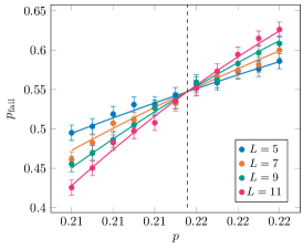
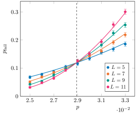
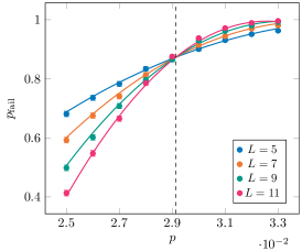
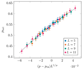
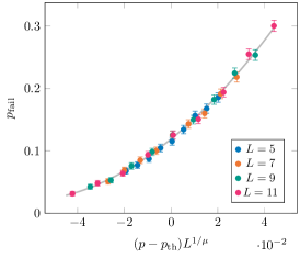
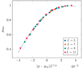
We use the fitting method described in [12] to understand the behaviour of the 3D toric code logical error rate for error rates significantly below threshold. Recall from Sec. V that we use the following ansatz:
| (59) |
we take the logarithm of both sides to obtain
| (60) |
For different values of , we plot as a function of and fit to a straight line to obtain gradients
| (61) |
where . Finally, take the logarithm of both sides of the above to give
| (62) |
We then plot as a function of and fit to a straight line to get and . Fig. 10 illustrates the above fitting procedure for code-capacity noise (no measurement errors) and for eight rounds of single-shot error correction.