A Case for Partitioned Bloom Filters

Abstract

In a partitioned Bloom Filter (PBF) the bit vector is split into disjoint parts, one per hash function. Contrary to hardware designs, where they prevail, software implementations mostly ignore PBFs, considering them worse than standard Bloom filters (SBF), due to the slightly larger false positive rate (FPR). In this paper, by performing an in-depth analysis, first we show that the FPR advantage of SBFs is smaller than thought; more importantly, by deriving the per-element FPR, we show that SBFs have weak spots in the domain: elements that test as false positives much more frequently than expected. This is relevant in scenarios where an element is tested against many filters. Moreover, SBFs are prone to exhibit extremely weak spots if naive double hashing is used, something occurring in mainstream libraries. PBFs exhibit a uniform distribution of the FPR over the domain, with no weak spots, even using naive double hashing. Finally, we survey scenarios beyond set membership testing, identifying many advantages of having disjoint parts, in designs using SIMD techniques, for filter size reduction, test of set disjointness, and duplicate detection in streams. PBFs are better, and should replace SBFs, in general purpose libraries and as the base for novel designs.

1 Introduction

A Bloom filter [1] is a probabilistic data structure to represent a set in a compact way. An element which has been inserted will always be reported as present; an element not in the set may erroneously be reported as present (i.e., false positives may arise), but the Bloom filter may be configured such that the probability of false positives may be as low as desired. Bloom filters are used in many settings, such as networking [2] and distributed systems [3].

A standard Bloom filter is a single array of $m$ bits over which $k$ independent hash functions range. When inserting an element, each of the $k$ functions is used to produce an index, and the corresponding bit is set. When querying, an element is considered present if all bits in the positions given by the $k$ hash functions are set.

A variant, partitioned Bloom filters, proposed by Mullin [4], divides the array into $k$ disjoint parts of size $m/k$ (assuming $m$ multiple of $k$). Each of the $k$ hash functions ranges over $m/k$, being used to set or test a bit in the corresponding part. The more obvious feature in partitioned Bloom filters is the complete independence of each of the $k$ parts and of each corresponding bit setting/testing. This has some obvious advantages, such as parallel access to each part, which has made partitioned Bloom filters widely adopted in hardware implementations [5, 6], where they are sometimes called parallel Bloom signatures.

A hybrid variant divides the filter in $k/h$ parts, with $h$ hash functions per part, such as a hardware implementation [7] where $k/h$ independent multi-port memory cores, each allowing $h$ accesses per cycle is used. An important consideration [6] for hardware designs is that using single-port SRAM, for the partitioned scheme, requires much less area than using $k$-ported SRAM for the standard scheme, or $h$-ported SRAM for the hybrid scheme, because the size of an SRAM cell increases quadratically with the number of ports. This seems to settle the standard-versus-partitioned choice for hardware designs, leading them to typically opt for the partitioned variant.

Concerning software implementations, standard Bloom filters prevail. The general feeling towards partitioned Bloom filters is that they are almost the same as standard ones, but produce slightly worse false positive rate (FPR), specially in small Bloom filters. This comes from the observation [8] that partitioned Bloom filters will have slightly more bits set than standard ones, and this slightly higher fill ratio (proportion of set bits) will result in a correspondingly higher FPR.

As we will demonstrate in this paper, the issue is more subtle, and this slight advantage comes at a substantial cost, including in the false positive rate itself. The main contributions of this paper are:

• Perform an in-depth analysis of the FPR in Bloom filters where we: provide a simpler explanation, compared with current literature, of why the standard formula is a strict lower bound of the true FPR; address the effect due to different hash functions colliding for a given element; obtain for the first time an exact formula for the per-element FPR, i.e., the expected FPR, for each specific element of the domain, over the range of filters that do not contain it.

• Point out the consequences for standard Bloom filters of the above hash collision problem, namely the occurrence of weak spots in the domain: elements which will be tested as false positives much more frequently than expected. This can be a problem, both for standard small capacity Bloom filters, or for blocked Bloom filters [9], and its unexpectedly frequent occurrence can be as surprising as the Birthday Problem [10].

• Expose pitfalls when using Double Hashing with standard Bloom filters, of which many widespread libraries seem to be unaware off, and contrast it with the robustness of partitioned Bloom filters in this matter.

• Survey usages for Bloom filters other than testing set membership, identifying many advantages that result from having disjoint parts that can be individually sampled, extracted, added or retired. We identify how the partitioned scheme leads to superior designs for SIMD techniques, testing set disjointness, reducing filter size, and duplicate detection in streams.

2 Bloom filters and the Birthday Problem

While most Bloom filters are used to represent large sets, in some scenarios small Bloom filters are used. If a small FPR is also wanted, the combination of a small $m$ and a (relatively) large $k$ will cause, for a standard Bloom filter, a non-negligible probability that two or more of the $k$ hash functions, applied to a given element, collide (produce the same index). Such a collision is illustrated in Figure 1, in yellow, where two of the 4 hash functions applied to $y$ produce the same index, resulting in a total of three bits being set for $y$, instead of the expected 4 bits. Such intra-element hash collisions are not normally illustrated (or discussed) in Bloom filter presentations, which just focus on inter-element collisions, such as the one between $x$ and $y$, in red.

In fact the surprisingly high probability of intra-element hash collisions is precisely an instance of the Birthday Problem, stated in 1927 by H. Davenport, as described by Coxeter [10]. The probability that, for a given element, two or more of the $k$ independent hash functions return the same value is:

$$1-{P(m,k)\over m^{k}},$$ (1)

where $P(m,k)$ denotes the $k$-permutations of $m$. We now give some examples.

Figure 1: Standard Bloom filter using 4 hash functions.

Sets of words in small strings

Mullin [12] used Bloom filters to store sets of words occurring in strings (e.g., titles and authors of articles), typically up to 15 words per string, with filters ranging from 32 up to 256 bits, the most common one being 96 bits, and using 8 hash functions per filter. With $m=96$ and $k=8$ two or more hash function will collide in one out of four cases (25.88%), where the FPR will be at least twice the expected from the classic formula (for filters that reached design capacity), or much higher than expected (for filters still far away from design capacity).

Packet forwarding

Whitaker and Wetherall [13] used small Bloom filters in packets to detect possible forwarding loops in experimental routing protocols. In this case 64 bit filters were used, with “4 bits set to one”. With $m=64$ and $k=4$ two or more hash function will collide 9.1 percent of the time. Interestingly, and different from the more normal usage, in this case a given element (node) is tested against many Bloom filters (packets), and instead of using $k$ hash functions for the element, a Bloom mask with exactly 4 ones at random positions is computed at start time, overcoming the collision problem.

Blocked Bloom filters

One problem with Bloom filters is the spreading of memory accesses, hurting performance. This is avoided by blocked Bloom filters [9], where the filter is divided into many blocks, each block a Bloom filter fitting into a single cache line (e.g., 512 bits), and using an extra hash function to select the block. For a very high precision filter, with $k=16$ and $m=512$, hash collisions will occur for 21 percent of elements, and even for a more normal setting of $k=8$, there will be collisions for 5.3 percent of elements. For an extreme performance BBF that requires a single memory access, using word sized blocks, $m=64$, for $k=8$ we have collisions 36 percent of time, or 9 percent of the time for the more reasonable $k=4$. So, the collision problem occurs in practice for BBFs. It should be emphasized that using blocking is the only way that Bloom filters can remain performance-wise competitive [14] with dictionary-based approaches (such as Cuckoo Filters [15], Morton Filters [16]), or Xor Filters [17]. Therefore, the scenario of a small Bloom filter (a block of a BBF) is important, even for scenarios with huge (on the whole) filters.

The above mentioned hash collision possibility is not a problem in partitioned Bloom filters because each of the $k$ functions is used to set/test bits in a different part. While in standard Bloom filters hash collisions will lead to bit collisions (the same bit being used for different functions), in partitioned Bloom filters such hash collisions will not lead to bit collisions. This is illustrated in Figure 2, which shows a partitioned Bloom filter using 4 parts, represented as a bidimensional bit array with one row per part. It can be seen that even if two of the 4 hash functions applied to $y$ produce the same value (column index), two different bits in the filter are set.

Figure 2: Partitioned Bloom filter using 4 hash functions, represented as a bidimensional bit array with one row per part.

So, while for partitioned Bloom filters, exactly $k$ distinct bits in the filter are accessed, in standard Bloom filters up to $k$ distinct bits are accessed (most times $k$ bits, but sometimes less than $k$ bits). As we will see, this makes the standard false positive formula incorrect, producing a value lower than the actual one, and complicating the exact false positive calculation (something that has been addressed before) but it also produces a non-uniform distribution of the FPR, with the occurrence of weak spots in the domain, something that we address here for the first time.

Interestingly, in the original proposal by Bloom [1] exactly $k$ bits are set/tested: “each message in the set to be stored is hash coded into a number of distinct bit addresses” and “where d is the number of distinct bits set to 1 for each message in the given set”. The original formula for the FPR is consistent with this behavior. This fact seems to have been mostly ignored in the literature, being one notable exception [18] “In [Bl70], the assumption was that the k locations are chosen without repetitions; it is also possible to allow repetitions, which makes the program simpler” and more recently [19] a comparison between the original proposal and standard Bloom filters.

The original Bloom proposal is not practical, as it demands some extra effort to ensure exactly $k$ distinct addresses, e.g., iterating over an unbounded family of hash functions until $k$ different values have been produced (with the need to compare each new value to all the previous ones); or a way to directly produce a pseudo-random $k$-permutation of $m$, keyed by the element. And even if little cost seems to be required [20], practitioners typically would not be aware of the problem or solution, and would not bother to address such minutiae. So, it is not surprising that what became adopted as standard Bloom filters differs from the original proposal.

Partitioned Bloom filters, which differ both from the original and the standard ones, not only are immune to the birthday problem (being in a sense more in the spirit of the original proposal) but are also practical to implement.

3 False positive analysis

We now do a theoretical analysis of the FPR, revisiting the Bloom’s analysis, the standard analysis, existing improvements to the standard analysis producing a correct formula, the formula for partitioned Bloom filters, and compare standard with partitioned Bloom filters. In the next section we present a novel per-element false positive analysis, showing how the expected FPR behaves for different elements in the domain.

3.1 Original Bloom’s analysis

Bloom’s analysis [1] states that the probability of a bit still being zero after $n$ elements are added is

$$\left(1-{k\over m}\right)^{n},$$ (2)

which, contrary to what sometimes is said, is correct, but for the original Bloom proposal where exactly $k$ distinct bits are set, and that the false positive rate is:

$$\left(1-\left(1-{k\over m}\right)^{n}\right)^{k}.$$ (3)

The analysis is almost correct, but it suffers from the same problem as the standard analysis below. But it is irrelevant for standard Bloom filters used in practice, as they differ from the original Bloom proposal.

3.2 Standard analysis

The standard analysis, by Mullin [4], and widely used, states that the probability of a bit still being zero after $n$ elements are added is

$$\left(1-{1\over m}\right)^{kn},$$ (4)

which is correct, and that the FPR is

$$F_{a}(n,m,k)=\left(1-\left(1-{1\over m}\right)^{kn}\right)^{k}.$$ (5)

which is only approximate, as we discuss below.

3.3 The exact formula for standard Bloom filters

There is one problem with the standard analysis, which has already been detected and corrected before. The standard analysis derives the FPR only as function of the mean fill ratio $p$, as $p^{k}$. Even though this gives a very good approximation for large Bloom filters, given the high concentration of the fill ratio around its mean [21], it is not an exact formula.

Exact formulas for standard Bloom filters were developed [22, 23], by deriving the probability distribution of the fill ratio and weighing the false positive rate incurred by each concrete fill ratio with the probability of it occurring. A similar result had already been derived [18], for a Bloom filter variant divided in pages (essentially, a blocked Bloom filter with typically large blocks), and a formula for the original Bloom filters was derived more recently [19].

A simpler strict lower bound argument

The standard formula, in Equation 5, has also been proven to be a strict lower bound for the true FPR [22] using considerations of conditional probability, and to be a lower bound [23] by resorting to Hölder’s inequality [24]. We now present a simpler and more elegant reasoning of why it is a strict lower bound. It results from a direct application of Jensen’s inequality [25]: for a convex function, such as $f(x)=x^{k}$ when $k>1$ and $x>0$, and for a non-constant random variable $R$, such as the fill ratio,

$$f(\operatorname{\mathbb{E}}[R])<\operatorname{\mathbb{E}}[f(R)].$$ (6)

This means that, for $k>1$, raising the expected fill ratio to the power of $k$, as done in the standard formula, produces a value always smaller than the expected value of the fill ratio raised to the power of $k$, which is what gives the exact average FPR.

As presented by the above mentioned works, computing the fill ratio distribution is an instance of the well known balls into bins experiment. It can be computed by resorting to the number of surjective functions from an $n$-set to an $i$-set, $e_{ni}$ [26], that can be directly derived using the inclusion-exclusion principle (in the complementary form) as:

$$e_{ni}=\sum_{j=0}^{i}(-1)^{j}{i\choose j}(i-j)^{n}.$$ (7)

The probability $B(n,m,i)$ of having exactly $i$ non-empty bins, after throwing $n$ balls randomly into $m$ bins is then:

$$B(n,m,i)={{m\choose i}e_{ni}\over m^{n}}.$$ (8)

The probability of having exactly $i$ bits set after inserting $n$ elements into an $m$ sized standard Bloom filter using $k$ hash functions is then:

$$S(n,m,k,i)=B(nk,m,i),$$ (9)

and the FPR for a standard Bloom filter is then:

$$F_{s}(n,m,k)=\sum_{i=1}^{m}S(n,m,k,i)\left({i\over m}\right)^{k}.$$ (10)

3.4 The exact formula for partitioned Bloom filters

As the $k$ parts are independently set/tested, the expected FPR is the product of the individual expected rates, and so computed as the one for each part to the power of $k$. For each part, the standard formula, with $k=1$, gives the exact part FPR, as the inequality in Equation 6 becomes an equality when $k=1$. So, for a partitioned Bloom filter of size $m$, made up of $k$ parts, each $m/k$ bits, the exact FPR when $n$ elements were inserted is given by:

$$F_{p}(n,m,k)=\left(1-\left(1-{k\over m}\right)^{n}\right)^{k},$$ (11)

which is much simpler than the exact formula for standard Bloom filters (as well as the exact formula for original Bloom filters [19]). Interestingly, it coincides with Bloom’s formula for his original proposal, while being exact.

This formula simplicity results from the conceptual simplicity: a partitioned Bloom filter can be seen as an AND of $k$ independent single-hash filters, all used for each insertion. It also translates to a simplicity of presentation, which is better, pedagogically, than standard Bloom filters, as it allows deriving a more complex (composite) concept in terms of a simpler one (single-hash filters).

3.5 Comparison with partitioned Bloom filters

Common folklore is that partitioned Bloom filters are not worth over standard ones [8]: “partitioned filters tend to have more 1’s than nonpartitioned filters, resulting in larger false positive probabilities”. But in spite of hash collisions decreasing the fill ratio, they increase the false positives for elements with collisions, and so the question is more subtle. Using the exact formulas for each case, Table I shows how partitioned and standard Bloom filters compare, namely the ratio of false positives $F_{p}/F_{s}$, for some combinations of $m$ and $k$ for filters at full capacity with $n=\frac{m}{k}\ln 2$.

We focus on small/medium sized filters for two reasons: 1) for large (plain) filters standard and partitioned variants exhibit almost the same FPR, being essentially indistinguishable; there is no point in comparing them and; 2) even if we want a large (on the whole) filter, the best performance will be achieved using a blocked Bloom filter, which will have relatively small blocks. The three sizes chosen (64, 512, and 4096 bits) are the more important ones for which it is meaningful to compare SBF and PBF. The first two, the word sized (64 bits) filter and the cache line sized (typically 512 bits) filter, the typical block in a BBF, are the more important ones. The last one (4096 bits) is still small enough such that some difference between SBFs and PBFs can be observed. The trio forms a sequence, each pair roughly separated by (almost) an order of magnitude (512/64 = 4096/512 = 8).

TABLE I: Comparison between partitioned and standard Bloom filters FPRs, for different combinations of $m$ and $k$, for filters at nominal occupation ($n=\frac{m}{k}\ln 2$), showing both the approximate ($F_{a}$) and the exact ($F_{s}$) values for standard filters, the value for partitioned filters ($F_{p}$) and the ratio $F_{p}/F_{s}$.

$m$	$k$	$F_{a}$	$F_{s}$	$F_{p}$	$F_{p}/F_{s}$
64	4	0.06244514	0.06423247	0.06676410	1.03941360
	8	0.00227672	0.00260362	0.00316870	1.21703762
512	4	0.06126247	0.06148344	0.06176528	1.00458411
	8	0.00375309	0.00381650	0.00389940	1.02172097
	16	0.00001409	0.00001513	0.00001661	1.09783475
4096	4	0.06233016	0.06235819	0.06239353	1.00056676
	8	0.00385474	0.00386284	0.00387308	1.00265094
	16	0.00001486	0.00001499	0.00001516	1.01143019

It can be seen that although partitioned filters have indeed slightly more false positives, the difference is less than what the standard formula ($F_{a}$) would suggest, and for all purposes irrelevant in practice. The largest increase is for the word sized Bloom filter with $k=8$, with 22% higher FPR. This extra 22%, which would be significant for other metrics like CPU usage, is not very relevant for the FPR, where mostly orders of magnitude matter. In this specific example, a PBF would have the same FPR as a standard filter by reducing the nominal capacity to compensate, roughly to $1/(1.22^{(1/8)})=0.975$, so by having only 2.5% less capacity than a standard BF. Moreover this combination $m=64$ and $k=8$ is an extreme case, more for illustration purposes, as it is not really suitable, allowing just a few elements in the filter or, in the case of a BBF, would lead to FPR degradation due to the danger of some blocks being too overloaded [9] (occupancies of blocks of a BBF follow a binomial distribution). BBFs normally aim for larger blocks of cache line size, typically with $m=512$, with word sized blocks not causing significant FPR degradation only for smaller values of $k$ (and larger FPRs).

Figure 3 plots the ratio of false positives $F_{p}/F_{s}$ over $m$, for some values of $k$. For filters of cache line size (512 bits) or larger, the difference between partitioned and standard filters is practically irrelevant, and only for cases that are not practically usable due to minuscule capacity (very small high accuracy filters) would the difference be significant.

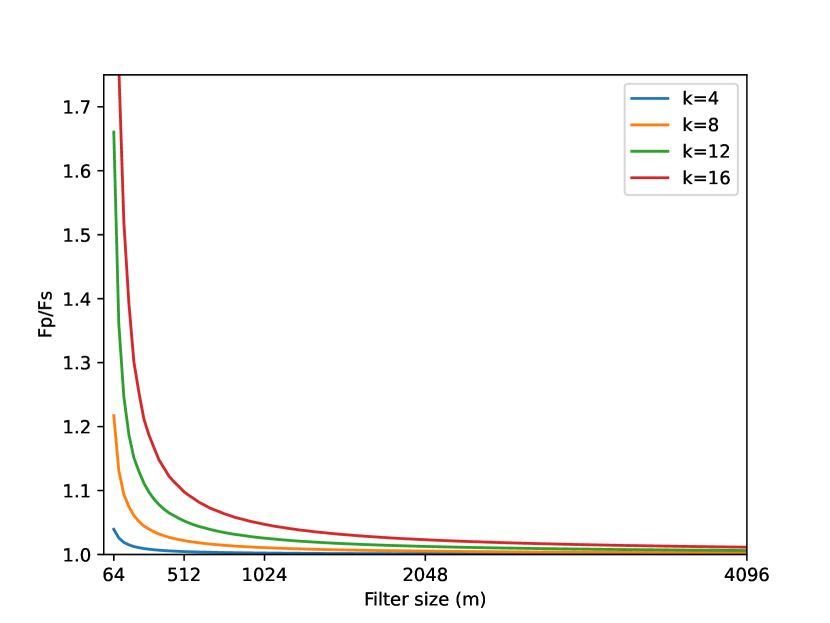
Figure 3: Ratio $F_{p}/F_{s}$ between partitioned and standard Bloom filters FPRs, for filters at nominal occupation ($n=\frac{m}{k}\ln 2$).

Table II shows the ratio of false positives $F_{p}/F_{s}$ for filters at different occupations (namely $1/4$, $1/2$, and $1/1$) relative to the nominal capacity. The ratio increases somewhat for word sized filters and small occupations, but those occupations for those filters are degenerate cases, with just a few elements inserted, and negligible FPR, whether for standard or partitioned filters.

TABLE II: Ratio between partitioned and standard Bloom filters FPR, $F_{p}/F_{s}$, for different combinations of $m$, $k$, and occupation (fraction of the nominal capacity $n=\frac{m}{k}\ln 2$).

		occupation
$m$	$k$	1/4	1/2	1/1
64	4	4.42059447	1.11720759	1.03941360
	8	8.91227883	1.77601565	1.21703762
512	4	1.00616297	1.00527287	1.00458411
	8	1.02790590	1.02512045	1.02172097
	16	1.13309283	1.11474124	1.09783475
4096	4	1.00069246	1.00064963	1.00056676
	8	1.00324437	1.00303940	1.00265094
	16	1.01404449	1.01313731	1.01143019

So, the average FPR is not relevant in practice for making a choice between standard versus partitioned Bloom filters. But as we discuss next, a more relevant issue is the distribution of false positives over the elements in the domain subject to being tested.

4 Weak spots in the domain

There are two ways that Bloom filters can be used, and two different points of view regarding false positives:

1. Filter point of view: having a filter, in which elements were inserted along time, test new elements using the filter.

2. Element point of view: for a specific element, test it against many different filters that show up, to see if the element is present in them.

The first usage is the more normal, for which we want to know the global average FPR. The second usage corresponds to the packet forwarding scenario, where at each node (representing an element) many different filters arrive (each one representing a path that a packet took to reach the node). For this second usage we want to know, for each specific element in the domain, the average FPR over all possible filters that do not include the element, for each given combination of $k$, $m$, and $n$. Particularly relevant is the question of whether this per-element rate is the same for all elements (the global average) or whether it is non-uniform, varying for different elements.

For partitioned Bloom filters, with $k$ independent parts, accessed by $k$ independent hash functions, the per-element FPR is the same for all elements, and equal to the global average. But for standard Bloom filters, the possibility of hash collisions makes some elements have less than $k$ independent bits to test. We have thus a non-uniform distribution of false positives: for a given element having $d<k$ different bit positions to test, the average FPR will be higher than for those elements for which no collisions occur. Elements suffering collisions are then weak spots in the domain: they will be considered more often than expected as belonging to filters against which they are tested. As we will see, for elements suffering several hash function collisions, the false positive rate can be more than one order of magnitude larger than expected. We now derive an exact formula for the per-element FPR.

4.1 Per-element false positive analysis

Consider a specific element $e$ of the domain, having $d$ different bit positions resulting from the $k$ independent hash functions, where $d\leq k$. We want to know the average FPR $F_{s}(n,m,k,d)$ when $e$ is tested against standard Bloom filters of size $m$ where a set of $n$ elements not containing $e$ was inserted.

A first observation is that the per-element rate cannot be obtained by simply going to the exact formula in Equation 10, where the fill ratio is raised to the power of $k$, and replacing $(i/m)^{k}$ with $(i/m)^{d}$, i.e.,

$$F_{s}(n,m,k,d)\neq\sum_{i=1}^{m}S(n,m,k,i)\left({i\over m}\right)^{d}.$$ (12)

The reason is that by saying that there are $d$ different positions, they are not independent, and we cannot use the independent testing assumption as for the $k$ positions. This can be seen by a simple example of a filter with $k=2$, $m=2$, $n=1$, and computing the FPR for elements with $d=2$ different bits. When considering the case $i=1$, i.e., one bit set in the filter, being the fill ratio $1/2$, for $d=2$ there is no possibility of a false positive, while using $(i/m)^{d}$ would give the erroneous $(1/2)^{2}=1/4$.

The correct formula for the probability of $d$ different bits being set when $i$ of the $m$ bits in the filter are set is:

$$\prod_{j=0}^{d-1}\frac{i-j}{m-j},$$ (13)

i.e., the first of the $d$ positions is one of the $i$ bits set, the second is one of the remaining $i-1$, the third one of the remaining $i-2$ and so on. The probability is zero for $d>i$.

The correct formula for the per-element FPR is then obtained by averaging over the different possible numbers of bits set, weighted by their probability of occurring, as before, resulting in:

$$F_{s}(n,m,k,d)=\sum_{i=1}^{m}S(n,m,k,i)\prod_{j=0}^{d-1}\frac{i-j}{m-j}.$$ (14)

Table III shows how the per-element FPR compares with the (global) average FPR, showing the ratio $F_{s}(n,m,k,d)/F_{s}(n,m,k)$ for different numbers of hash collision $c=k-d$, from no collision ($d=k$) up to three collisions ($d=k-3$), for filters at different occupations (ratios relative to nominal capacity $n=\frac{m}{k}\ln 2$).

TABLE III: Ratio between per-element and global FPR for standard Bloom filters, $F_{s}(n,m,k,d)/F_{s}(n,m,k)$, for different combinations of $m$, $k$, and hash collisions $c=k-d$, for filters at different occupations.

			collisions
occupation	$m$	$k$	0	1	2	3
1/1	64	4	0.91	1.88	3.85	7.78
		8	0.59	1.39	3.25	7.47
	512	8	0.95	1.92	3.89	7.88
		16	0.79	1.62	3.31	6.78
1/2	64	4	0.76	3.21	12.92	50.00
		8	0.14	1.09	7.50	47.38
	512	8	0.87	3.09	10.87	38.10
		16	0.56	2.03	7.41	26.86
1/4	64	4	0.38	5.90	74.86	804.25
		8	0.00	0.07	4.45	134.33
	512	8	0.74	5.03	33.76	224.42
		16	0.23	1.87	15.28	123.08

It can be seen that the FPR increases noticeably with the number of hash collisions that occur for the element being tested, in relation to the global average rate for the filter. This effect is more prevalent for small occupations, with the FPR reaching two orders of magnitude larger than the global average for $1/4$ occupation and three collisions. This may cause surprises in scenarios where a filter is dimensioned with some expectations about the FPR over its lifetime, from empty to full. Some elements will incur much more false positives than what planned for, if using either the standard or exact formula for the global average.

4.2 Probability distribution of hash collisions

The question of how frequent are those weak spots in the domain, specially the “very weak” spots having more than one hash collision is easily answered. The probability of an element being a weak spot is an instance of the birthday problem, as discussed above, with value given by Equation 1. For an $m$ sized Bloom filter, the probability of the $k$ hashes resulting in $d$ different bits (i.e., $c=k-d$ collisions) is an instance of the balls into bins experiment, with value $B(k,m,d)$ as given by Equation 8.

Table IV shows the probability of having some (one or more) hash collisions, and of having exactly $0\leq c\leq 3$ collisions, for some combinations of $k$ and $m$.

TABLE IV: Probability of having some hash collision(s) and of having exactly $0\leq c\leq 3$ hash collisions, for some combinations of $k$ and $m$.

		collisions
$m$	$k$	some	0	1	2	3
64	4	0.0911	0.9089	0.0894	0.0017	0.0000
	8	0.3660	0.6340	0.3115	0.0510	0.0034
512	8	0.0535	0.9465	0.0525	0.0010	0.0000
	16	0.2108	0.7892	0.1905	0.0192	0.0011

It can be seen that collisions happen frequently not only in word sized filters (36% of elements for $m=64$ and $k=8$) but also for the important case of cache line sized blocks ($m=512$) in blocked Bloom filters, reaching 21% for very high accuracy ($k=16$) filters. Two collisions can happen with non-negligible frequency, in 5 percent of elements for the word sized filters with $k=8$, or in two percent of elements in the ($m=512$, $k=16$) case. And while three collisions is indeed very rare, 3 in a thousand for the ($m=64$, $k=8$) filter or one in a thousand for the ($m=512$, $k=16$) filter, this is no consolation when those “unlucky” elements are subject to being tested against many filters.

We now combine the per-element FPR values (as shown in Table III) with the probabilities of their occurrence (as shown in Table IV. Figure 4 plots the inverse of the tail distribution (ignoring values with very low probability of occurrence) of the ratio between per-element and global FPR for standard Bloom filters, $F_{s}(n,m,k,d)/F_{s}(n,m,k)$, for different combinations of $m$ and $k$, for filters at nominal occupation ($n=\frac{m}{k}\ln 2$). From it, it can be seen that, e.g., for a $m=512$, $k=16$ high accuracy filter, for one in one thousand elements the FPR will be more than 6 times the global FPR, and for almost one in a million elements it will be almost 30 times the global FPR.

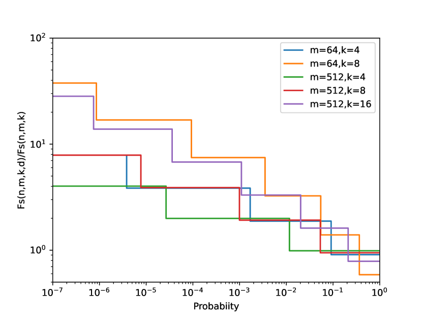
Figure 4: Inverse of tail distribution of ratio between per-element and global FPR for standard Bloom filters, $F_{s}(n,m,k,d)/F_{s}(n,m,k)$, for different combinations of $m$, $k$, for filters at nominal occupation ($n=\frac{m}{k}\ln 2$).

5 Pitfalls in double hashing

One technique used to improve performance, by avoiding the need to compute $k$ hash functions, is to resort to double hashing, which amounts to using two hash functions $\{h_{1},h_{2}\}$, to simulate $k$ hash functions. In the more naive form it amounts to computing $g_{0},\ldots,g_{k-1}$ as:

$$g_{i}(x)=h_{1}(x)+ih_{2}(x)\mod m$$

The first time that double hashing was applied to Bloom filters seems to have been by Dillinger and Manolios [27], for model checking. It was popularized after Mitzenmacher [8] showed that it could be used to implement a Bloom filter without any loss in the asymptotic false positive probability, and experimentally validating it for medium sized Bloom filters, starting with $m=10000$ bits. However, small Bloom filters were not considered (e.g., a 512 bits block in a BBF) and, as usual, only the global FPR was considered.

Here we address small filters and the possibility of a non-uniform distribution of false positives, with weak spots in the domain. We show that standard Bloom filters, but not partitioned ones, are prone to even more problematic weak spots caused by the use of double hashing. Although more sophisticated variants, like enhanced double hashing or triple hashing have been proposed, naive doubling hashing in particular has become relatively popular, and can be found in many Bloom filter implementations. Therefore, these issues have practical consequences.

Dillinger’s PhD dissertation [28], which includes a detailed study of different forms of double and triple hashing, already recognized the existence of pitfalls, specially in naive double hashing. It identified three issues, which we now show that only affect standard, but not partitioned, Bloom filters.

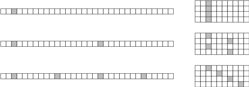
Figure 5: Effects of double hashing when inserting an element $x$ in a standard (left) versus partitioned (right) Bloom filter, when $b=h_{2}(x)$ is 0, $1/2$, or $1/4$ the size of the vector being indexed (filter or part).

Issue 1

Some possibilities for $b=h_{2}(x)$ can result in many repetitions of the same index. The worse case would be if $b=0$ (mod $m$), in which case all indices would be the same, but the existence of common factors between $b$ and $m$ also causes problems. Figure 5 shows some examples, with $b=0$, $b=m/2$ and $b=m/4$. On the left, for standard Bloom filters, there is overwhelming index collision, which causes bit collisions, resulting in very weak spots. In a BBF with 512 bit blocks, one out of 512 elements in the domain will have a single bit set/tested, resulting in a disastrous $1/2$ probability of them being tested as a false positive in filters at nominal capacity ($1/2$ fill ratio). Then, one out 512 elements $1/4$ probability, and so on. For partitioned Bloom filters, index collisions do not cause bit collisions, resulting always in $k$ bits being set/tested.

Issue 2

The indices generated by double hashing, used to index a standard Bloom filter are treated as a set, not a sequence, and we can compute the same set going “forward” or going “backward”. Two elements $x$ and $y$, can have a full overlap of the $k$ bits without both $h_{1}$ and $h_{2}$ colliding, if $h_{1}(y)=h_{1}(x)+(k-1)h_{2}(x)\mod m$ and $h_{2}(y)=m-h_{2}(x)\mod m$. For a partitioned Bloom filter, such overlap does not occur, as the different parts are indexed in order, and so we have effectively a sequence of indices. Figure 6 illustrates the full overlap between $x$ and $y$, for a standard Bloom filter and the absence of overlap in a partitioned Bloom filter.

Figure 6: Full overlap between $x$ and $y$ when using double hashing in a standard Bloom filter, when $h_{1}(y)=h_{1}(x)+(k-1)h_{2}(x)\mod m$ and $h_{2}(y)=m-h_{2}(x)\mod m$ (left), and the lack of such overlap in a partitioned Bloom filter (right).

Issue 3

Using double hashing in a standard Bloom filter is prone to partial overlapping of the $k$ indices, namely when $h_{2}(x)=h_{2}(y)\mod m$. This is illustrated in Figure 7. In the same figure, it can be seen that in partitioned Bloom filters such overlap does not occur.

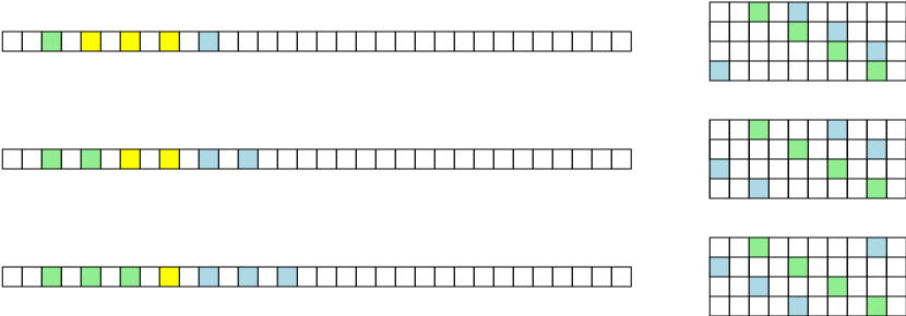
Figure 7: Partial overlap (yellow) between $x$ (green) and $y$ (blue) when using double hashing in a standard Bloom filter, when $h_{2}(x)=h_{2}(y)\mod m$ (left), and the lack of such overlap in a partitioned Bloom filter (right).

Standard Bloom filters are thus subject to these anomalies, the more serious being the possibility of extreme weak spots, if naive double hashing is used. In theory, Issue 1 (which causes weak spots) is easy to overcome, by ensuring there are no collisions, e.g., in the popular case when $m$ is a power of two by restricting $b=h_{2}(x)$ to produce odd numbers. In practice, implementers have been sold the idea that double hashing can be used harmlessly, and commonly do not take precautions, namely when the filter is parameterized, being $m$ arbitrary and possibly small. This has occurred even in mainstream libraries, such as in Google Core Libraries for Java [29]. Partitioned Bloom filters have the advantage of not being subject to such weak spots, and thus are robust to naive double hashing implementations.

It should be noted that if Issue 1 is addressed, the impact of double hashing on the global FPR is larger for partitioned Bloom filters than for the standard ones. This impact comes from the probability of the pair of indices for one element colliding with the pair from another element, i.e., $h_{1}(x)=h_{1}(y)$ and $h_{2}(x)=h_{2}(y)$ (modulo vector size). Between two elements it is $1/m^{2}$ for standard Bloom filters and $1/(m/k)^{2}$ for partitioned.

In practice, for large Bloom filters the contribution of double hashing for the global FPR is negligible, unless high accuracy filters are wanted, in which case care must be taken and triple hashing may be needed. For small filters, or in general when BBFs are used, neither double nor triple hashing should be used, as only a few bits per index are needed, and a single hash word can be split to obtain the $k$ indices. Concretely, in a BBF with 512 bit blocks and $k=8$, we need 9 bits per index for standard and 6 bits per index for partitioned filters. This means that a partitioned scheme needs $6*8=48$ bits per block and a single 64 bit hash word is enough for filters up to $2^{64-48}=65536$ blocks, i.e., $2^{25}=33554432$ bits, while if standard filters are used $9*8=72$ bits per block are needed and a 64 bit hash word is not enough even for small filters. This reinforces the superiority of partitioned Bloom filters over standard ones.

6 The flexibility advantage of disjoint parts

Regardless of the FPR itself, the disjointness of the parts in a partitioned Bloom filter provides several advantages over standard filters, either in terms of obtaining fast implementations or making the partitioned scheme more flexible to be used in more scenarios, or as the base for further extensions. Each disjoint part can be sampled, extracted, added, or retired individually, leading to interesting outcomes. We conclude our case by surveying some of these usages and advantages.

6.1 Fast Bloom filters through SIMD

In addition to improving memory accesses, through blocked Bloom filters, another way to improve performance is to use Single Instruction Multiple Data (SIMD) processor extensions, to test multiple bits in a single processor cycle. However, standard Bloom filters are not directly suitable to SIMD, because the $k$ bits are spread over memory, needing an extra gather step to collect and place them appropriately, causing some slowdown.

A sophisticated SIMD approach [30] for standard Bloom filters uses precisely gather instructions to collect bits spread over memory. It achieves higher throughput, by testing different hashes of different elements at each step, but not lower latency of individual query operations.

Even using BBFs based on standard Bloom filter blocks is not directly suitable to SIMD, because the $k$ bits are not placed over independent disjoint parts of the cache line (e.g., words) to be used together as a vector register. When introducing BBFs the authors already discussed SIMD usage, and to overcome this problem they propose using a table of $k$ bit block-sized patterns. However, to avoid collisions between elements when indexing, the table cannot be too small, competing for cache usage.

Partitioned Bloom filters are more directly suitable to SIMD. A blocked Bloom filter using the partitioned scheme, with cache-line sized blocks and word sized parts is perfect for SIMD, and arises as the natural combination of blocking and partitioning. This is precisely what Ultra-Fast Bloom Filters [31] have recently proposed. We may conjecture that, had partitioned Bloom filters been the norm at the time when BBFs were introduced, this combination could have appeared one decade earlier.

6.2 Set disjointness

Bloom filters can also be used for set union and intersection. Unlike for union (bitwise or) which is exact, intersection of filters (bitwise and) over-represents the filter for the intersection: given sets $S_{1}$ and $S_{2}$, we have $F(S_{1})\land F(S_{2})\geq F(S_{1}\cap S_{2})$. In addition to testing for the presence of some element, an important use case is testing for set disjointness, i.e., that the intersection is an empty set. An example is checking whether two sets of addresses, representing a read-set and a write-set are disjoint, when implementing transactional memory.

Using standard Bloom filters, being sure that the sets are disjoint is only possible when the resulting filter intersection is completely empty (all zeroes). Having less than $k$ one bits is not enough, due to weak spots. As already noticed [32], even if the intersection result had a single bit it could be (even if extremely unlikely) due to an element, present in both sets, having the $k$ hash functions collide.

Partitioned Bloom filters are much better suited for testing set disjointness, as it is enough that one of the $k$ parts of the filter intersection is empty to conclude that the set intersection is empty. This was already exploited [5] for speculative multithreading. A comparison of set disjoitness testing concluded [32] that the probability of false set-overlap reporting was substantially smaller for partitioned Bloom filters than standard Bloom filters. This probability, for standard ($P_{s}$) and partitioned ($P_{p}$) $m$ sized filters with $k$ hash functions, representing sets with $n_{1}$ and $n_{2}$ elements, compares as:

$$P_{s} =1-\left(1-{1\over m}\right)^{k^{2}n_{1}n_{2}}$$

$$>1-\left(1-{k\over m}\right)^{n_{1}n_{2}}$$

$$>\left(1-\left(1-{k\over m}\right)^{n_{1}n_{2}}\right)^{k}=P_{p}.$$

This is intuitively easy to understand: the probability of a false set-overlap for a standard $m$ sized filter, due to some of the $k*n_{1}*k*n_{2}$ pairs of indices colliding, is greater than the probability of such an overlap in a given $m/k$ sized part for the partitioned scheme, which is substantially greater than the probability that there is an overlap in each of the $k$ parts.

6.3 Size reduction

Sometimes it is useful to obtain a smaller sized, lower accuracy, version of a Bloom filter. Either because the filter was overdimensioned and we do not need the resulting overly high accuracy; or we want to obtain an explicitly lower accuracy view (but enough for some purpose), e.g., to ship over the network, wanting to save bandwidth.

A standard Bloom filter is not suitable for this purpose because of the mingling of bits from different hash functions. What can be done is to use the same $k$ hashes, but remap the indices to a smaller $m^{\prime}$ sized vector (preferably with $m$ some multiple of $m^{\prime}$), moving the bit in position $i$ to $i$ modulo $m^{\prime}$, and using modulo $m^{\prime}$ indexing for the new filter. The problem is that the resulting fill rate renders the filter, when not immediately useless, having an overly high FPR, when comparing with the optimal for the new smaller size and the same number of elements [33].

TABLE V: Comparison between Bloom filter variants and common fingerprint-based approaches.

	Bloom				fingerprint
	SBF	PBF	SBBF	PBBF	Cuckoo	Xor	Ribbon	BFF
weak spots	yes	no	yes	no	no	no	no	no
incremental construction	yes	yes	yes	yes	yes	no	no	no
delete possible	no	no	no	no	yes	no	no	no
construction time	normal	normal	fast	fast	slow	slow	normal–slowest	normal
query time	normal	normal	fastest	fastest	fast	fast	normal	fast
memory usage	high	high	highest	highest	normal	low	low-lowest	lower
trivial intersection over-representation	high	low	high	low	-	-	-	-
suitable for trivial disjointness test	no	yes	no	yes	-	-	-	-
extract lower accuracy views	no	yes	no	yes	immut.	immut.	immut.	immut.

Partitioned Bloom filters are much better for this purpose. Due to the disjointness of the $k$ parts, we can simply consider the first $k^{\prime}$ parts as a smaller Bloom filter, e.g., to be shipped elsewhere. For the worst case of a filter already at full capacity, the new one will provide the optimal FPR for the new smaller size. Considerable size reductions are viable, which would render a standard Bloom filter useless due to the fill rate approaching 1. The same paper proposes Block-partitioned Bloom filters, composed of several blocks (each block a standard filter, with insertions in each block, and using AND for queries), to be able to extract some blocks as a new filter. It mentions that maximum size flexibility is achieved by using one hash per block, i.e., by using a partitioned Bloom filter.

6.4 Duplicate detection in streams

Bloom filter based approaches to achieve queries over a sliding window of an infinite stream tend to be space inefficient. Traditionally they have been based either on some variation of Counting Bloom filters [34], on storing the insertion timestamp [35], or using several disjoint segments which can be individually added and retired, one example being Double Buffering [36]. This uses a pair of active and warm-up Bloom filters, using the active for queries and inserting in both until the warm-up is half-full, at which point it becomes the active, the previous active is discarded and a new empty warm-up is added.

While with standard Bloom filters a segment must be a whole filter, partitioned Bloom filters can be used as a base for better designs, in which each disjoint part can be treated as a segment. Age-Partitioned Bloom Filters [37] use $k+l$ (for some configurable $l$) parts in a circular buffer, using the $k$ more “recent” parts for insertions, discarding (zeroing) the “oldest” part after each generation (batch of insertions), and testing for the presence of $k$ adjacent matches for queries. This is the currently best Bloom filter based design for querying a sliding window over a stream. As for the other usages, starting from partitioned instead of standard filters was essential to be able to reach this new design.

7 Comparison

Partitioned Bloom filters may have several feature advantages, compared with the standard, but is it enough for them to be competitive with alternative approaches? A common view is that Bloom filters have been superseded by fingerprint-based mechanisms, such as Cuckoo [15] or Xor [17] filters. This is not necessarily the case: while that is true if the main concern is memory consumption and high accuracy, for moderate accuracy and when query time is important but memory less of a concern, Bloom filters, in blocked variants, remain the best [14].

We now summarize how the Bloom filter variants compare among themselves, and with some fingerprint-based approaches: the well known Cuckoo and Xor filters, and two recent state-of-the-art mechanisms, Ribbon filters [38] and binary fuse filters (BFF) [39]. Table V presents a feature-wise and qualitative comparison of filters (detailed quantitative results can be found elsewhere [17, 38, 39]). The columns, from left to right depict Bloom filters, in standard and partitioned variants, blocked Bloom filters using either standard or partitioned filters in blocks, and then fingerprint-based mechanisms: Cuckoo, Xor, Ribbon and binary fuse filters.

From all mechanisms, only standard Bloom filters (normal or blocked) suffer from the weak-spots problem in the per-element FPR distribution. Bloom approaches and cuckoo filters allow an incremental (progressive) construction, starting from an empty set, essential for an “online” operation. The others, XOR-probe based filters, are immutable, having to be built from a given set. Cuckoo filters also allow deletes (Counting Bloom Filters [40] allow deletes but consume too much memory).

Except for Ribbon, most fingerprint-based mechanisms are fast for queries, but lose to BBFs, which are also the fastest for construction. Cuckoo and Xor filters are slow to build. Fingerprint-based mechanisms are better in memory usage, specially for high accuracy filters, in which case BBFs start to become too memory hungry, leading to the need for large blocks or multiblocking [9]. If incremental construction is not needed, the two recent mechanisms are very appealing, BFF as very good both in memory usage and query speed, and Ribbon filters by being very configurable, allowing the lowest memory usage of all.

Where partitioned Bloom filters shine (whether plain or blocked variants) is in allowing extra features, such as trivial intersections leading to less over-representation than standard Bloom filters, or being suitable for trivial disjoitness tests (e.g., for read/write sets in transactional memory). Cuckoo filters could allow such tests, but not in the trivial way Bloom approaches allow, while the XOR-probe based filters do not allow intersections at all. Finally, partitioned Bloom filters allow extracting lower accuracy views, which can themselves be used as first class filters (allowing further insertions) while the fingerprint-based filters (including Cuckoo filters) only allow obtaining immutable views.

8 Conclusions

Frequently, a focus on one small difference in one quantitative aspect misses the whole picture. Partitioned Bloom filters have thus been considered worse than standard, and frequently not adopted, due to having slightly more false positives. This is ironic given that the difference amounts to a negligible variation of capacity, for the same FPR.

In this paper we have shown how much simpler, elegant, robust and versatile partitioned Bloom filters are. The simplicity of the exact formula results from the conceptual simplicity of them being essentially the AND of single-hash filters. Standard Bloom filters have a more complex nature due to the possibility of intra-element hash collisions, with a resulting complex exact formula, normally approximated, leading sometimes to surprises.

But essentially, we have shown how standard Bloom filters exhibit a non-uniform distribution of the false positive probability, with weak spots in the domain: elements that are reported much more frequently as false positives than expected. This is an aspect than has been neglected from the literature. Moreover, the issue of weak spots is much aggravated when naive double hashing is used. Even though easily circumventable, many libraries, including mainstream ones, suffer from this anomaly. The lesson seems to be that practitioners frequently skim over published results, failing to notice subtle problems. Partitioned Bloom filters have a uniform distribution of false positives over the domain, with no weak spots, even if naive double hashing is used. Moreover, the need for less hash bits makes such schemes less warranted.

Finally, going beyond set-membership test, by surveying other usages, the flexibility of being able to sample, extract, add or retire individual parts becomes clear, showing the partitioned scheme to be better. Like the hardware community already did, partitioned Bloom filters should be widely adopted by software implementers, and used as a better starting point for new designs, replacing standard Bloom filters as the new normal.

Paulo Sérgio Almeida is an assistant professor at University of Minho, and a senior researcher at HASLab / INESC TEC. He obtained a MSc degree from University of Porto in 1994 and a PhD degree in Computer Science from Imperial College London in 1998. His research activities have been in the area of distributed systems. Some main contributions have been in causality tracking mechanisms, eventually consistent databases, and fault-tolerant distributed aggregation algorithms. Other subjects have been Bloom filters and distributed algorithms in graphs. For some years the main focus of research has been on CRDTs (Conflict-free Replicated Data Types), with some results being the development of both pure operation-based and delta-state based CRDTs. Recently he has been revisiting Bloom filters.

References

- [1] B. H. Bloom, “Space/time trade-offs in hash coding with allowable errors,” Communications of the ACM, vol. 13, no. 7, pp. 422–426, 1970.
- [2] A. Broder and M. Mitzenmacher, “Network applications of bloom filters: A survey,” Internet mathematics, vol. 1, no. 4, pp. 485–509, 2004.
- [3] S. Tarkoma, C. E. Rothenberg, and E. Lagerspetz, “Theory and practice of bloom filters for distributed systems,” IEEE Communications Surveys & Tutorials, vol. 14, no. 1, pp. 131–155, 2012.
- [4] J. K. Mullin, “A second look at bloom filters,” Communications of the ACM, vol. 26, no. 8, pp. 570–571, 1983.
- [5] L. Ceze, J. Tuck, J. Torrellas, and C. Cascaval, “Bulk disambiguation of speculative threads in multiprocessors,” ACM SIGARCH Computer Architecture News, vol. 34, no. 2, pp. 227–238, 2006.
- [6] D. Sanchez, L. Yen, M. D. Hill, and K. Sankaralingam, “Implementing signatures for transactional memory,” in 40th Annual IEEE/ACM International Symposium on Microarchitecture (MICRO 2007). IEEE, 2007, pp. 123–133.
- [7] S. Dharmapurikar, P. Krishnamurthy, T. Sproull, and J. Lockwood, “Deep packet inspection using parallel bloom filters,” in High performance interconnects, 2003. proceedings. 11th symposium on. IEEE, 2003, pp. 44–51.
- [8] A. Kirsch and M. Mitzenmacher, “Less hashing, same performance: Building a better bloom filter,” Random Struct. Algorithms, vol. 33, no. 2, pp. 187–218, 2008.
- [9] F. Putze, P. Sanders, and J. Singler, “Cache-, hash-, and space-efficient bloom filters,” ACM Journal of Experimental Algorithmics, vol. 14, 2009. [Online]. Available: https://doi.org/10.1145/1498698.1594230
- [10] W. W. Rouse Ball. Revised by H. S. M. Coxeter, Mathematical Recreations and Essays, 11th ed. Macmillan, 1939.
- [11] P. Blog, “Who created the birthday problem, and even one more version,” https://pballew.blogspot.com/2011/01/who-created-birthday-problem-and-even.html, 2011 (accessed May 26, 2020).
- [12] J. K. Mullin, “Accessing textual documents using compressed indexes of arrays of small bloom filters,” The Computer Journal, vol. 30, no. 4, pp. 343–348, 1987.
- [13] A. Whitaker and D. Wetherall, “Forwarding without loops in icarus,” in Open Architectures and Network Programming Proceedings, 2002 IEEE. IEEE, 2002, pp. 63–75.
- [14] H. Lang, T. Neumann, A. Kemper, and P. A. Boncz, “Performance-optimal filtering: Bloom overtakes cuckoo at high-throughput,” Proc. VLDB Endow., vol. 12, no. 5, pp. 502–515, 2019. [Online]. Available: http://www.vldb.org/pvldb/vol12/p502-lang.pdf
- [15] B. Fan, D. G. Andersen, M. Kaminsky, and M. Mitzenmacher, “Cuckoo filter: Practically better than bloom,” in Proceedings of the 10th ACM International on Conference on emerging Networking Experiments and Technologies, CoNEXT 2014, Sydney, Australia, December 2-5, 2014, 2014, pp. 75–88. [Online]. Available: https://doi.org/10.1145/2674005.2674994
- [16] A. Breslow and N. Jayasena, “Morton filters: Faster, space-efficient cuckoo filters via biasing, compression, and decoupled logical sparsity,” PVLDB, vol. 11, no. 9, pp. 1041–1055, 2018. [Online]. Available: http://www.vldb.org/pvldb/vol11/p1041-breslow.pdf
- [17] T. M. Graf and D. Lemire, “Xor filters,” ACM J. Exp. Algorithmics, vol. 25, pp. 1–16, 2020. [Online]. Available: https://doi.org/10.1145/3376122
- [18] U. Manber and S. Wu, “An algorithm for approximate membership checking with application to password security,” Information Processing Letters, vol. 50, no. 4, pp. 191–197, 1994.
- [19] F. Grandi, “On the analysis of bloom filters,” Inf. Process. Lett., vol. 129, pp. 35–39, 2018. [Online]. Available: https://doi.org/10.1016/j.ipl.2017.09.004
- [20] C. S. Roberts, “Partial-match retrieval via the method of superimposed codes,” Proceedings of the IEEE, vol. 67, no. 12, pp. 1624–1642, 1979.
- [21] M. Mitzenmacher, “Compressed bloom filters,” IEEE/ACM Transactions on Networking (TON), vol. 10, no. 5, pp. 604–612, 2002.
- [22] P. Bose, H. Guo, E. Kranakis, A. Maheshwari, P. Morin, J. Morrison, M. Smid, and Y. Tang, “On the false-positive rate of bloom filters,” Information Processing Letters, vol. 108, no. 4, pp. 210 – 213, 2008. [Online]. Available: http://www.sciencedirect.com/science/article/B6V0F-4SMWFJ6-1/2/5f479ecc8eea9b5b67869b97a54c16b6
- [23] K. Christensen, A. Roginsky, and M. Jimeno, “A new analysis of the false positive rate of a bloom filter,” Information Processing Letters, vol. 110, no. 21, pp. 944–949, 2010.
- [24] O. Hölder, “Ueber einen mittelwertsatz,” Nachrichten von der Königl. Gesellschaft der Wissenschaften und der Georg-Augusts-Universität zu Göttingen, no. 2, pp. 38–47, 1889.
- [25] J. L. W. V. Jensen, “Sur les fonctions convexes et les inégalités entre les valeurs moyennes,” Acta mathematica, vol. 30, pp. 175–193, 1906.
- [26] F. Gerrish, “63.29. surjections from an m-set to an n-set,” The Mathematical Gazette, vol. 63, no. 426, pp. 259–261, 1979.
- [27] P. C. Dillinger and P. Manolios, “Fast and accurate bitstate verification for SPIN,” in Model Checking Software, 11th International SPIN Workshop, Barcelona, Spain, April 1-3, 2004, Proceedings, ser. Lecture Notes in Computer Science, S. Graf and L. Mounier, Eds., vol. 2989. Springer, 2004, pp. 57–75. [Online]. Available: https://doi.org/10.1007/978-3-540-24732-6_5
- [28] P. C. Dillinger, “Adaptive approximate state storage,” Ph.D. dissertation, Northeastern University, 2010.
- [29] D. Andreou and K. A. Kluever, “BloomFilterStrategies in google core libraries for java,” https://github.com/google/guava/blob/master/guava/src/com/google/common/hash/BloomFilterStrategies.java, 2011 (accessed September 8, 2020).
- [30] O. Polychroniou and K. A. Ross, “Vectorized bloom filters for advanced SIMD processors,” in Tenth International Workshop on Data Management on New Hardware, DaMoN 2014, Snowbird, UT, USA, June 23, 2014, A. Kemper and I. Pandis, Eds. ACM, 2014, pp. 6:1–6:6. [Online]. Available: https://doi.org/10.1145/2619228.2619234
- [31] J. Lu, Y. Wan, Y. Li, C. Zhang, H. Dai, Y. Wang, G. Zhang, and B. Liu, “Ultra-fast bloom filters using SIMD techniques,” IEEE Trans. Parallel Distrib. Syst., vol. 30, no. 4, pp. 953–964, 2019. [Online]. Available: https://doi.org/10.1109/TPDS.2018.2869889
- [32] M. C. Jeffrey and J. G. Steffan, “Understanding bloom filter intersection for lazy address-set disambiguation,” in SPAA 2011: Proceedings of the 23rd Annual ACM Symposium on Parallelism in Algorithms and Architectures, San Jose, CA, USA, June 4-6, 2011 (Co-located with FCRC 2011), R. Rajaraman and F. M. on the Heath, Eds. ACM, 2011, pp. 345–354. [Online]. Available: https://doi.org/10.1145/1989493.1989551
- [33] O. Papapetrou, W. Siberski, and W. Nejdl, “Cardinality estimation and dynamic length adaptation for bloom filters,” Distributed Parallel Databases, vol. 28, no. 2-3, pp. 119–156, 2010. [Online]. Available: https://doi.org/10.1007/s10619-010-7067-2
- [34] F. Bonomi, M. Mitzenmacher, R. Panigrahy, S. Singh, and G. Varghese, “An improved construction for counting bloom filters,” in Algorithms - ESA 2006, 14th Annual European Symposium, Zurich, Switzerland, September 11-13, 2006, Proceedings, 2006, pp. 684–695. [Online]. Available: https://doi.org/10.1007/11841036_61
- [35] L. Zhang and Y. Guan, “Detecting click fraud in pay-per-click streams of online advertising networks,” in 28th IEEE International Conference on Distributed Computing Systems (ICDCS 2008), 17-20 June 2008, Beijing, China, 2008, pp. 77–84. [Online]. Available: https://doi.org/10.1109/ICDCS.2008.98
- [36] F. Chang, K. Li, and W. Feng, “Approximate caches for packet classification,” in Proceedings IEEE INFOCOM 2004, The 23rd Annual Joint Conference of the IEEE Computer and Communications Societies, Hong Kong, China, March 7-11, 2004, 2004, pp. 2196–2207. [Online]. Available: https://doi.org/10.1109/INFCOM.2004.1354643
- [37] A. Shtul, C. Baquero, and P. S. Almeida, “Age-partitioned bloom filters,” CoRR, vol. abs/2001.03147, 2020. [Online]. Available: http://arxiv.org/abs/2001.03147
- [38] P. C. Dillinger and S. Walzer, “Ribbon filter: practically smaller than bloom and xor,” CoRR, vol. abs/2103.02515, 2021. [Online]. Available: https://arxiv.org/abs/2103.02515
- [39] T. M. Graf and D. Lemire, “Binary fuse filters: Fast and smaller than xor filters,” ACM J. Exp. Algorithmics, vol. 27, pp. 1.5:1–1.5:15, 2022. [Online]. Available: https://doi.org/10.1145/3510449
- [40] L. Fan, P. Cao, J. Almeida, and A. Z. Broder, “Summary cache: a scalable wide-area web cache sharing protocol,” IEEE/ACM Trans. Netw., vol. 8, no. 3, pp. 281–293, 2000.