Birth and destruction of collective oscillations in a network of two populations of coupled type 1 neurons

Abstract

We study the macroscopic dynamics of large networks of excitable type 1 neurons composed of two populations interacting with disparate but symmetric intra- and inter-population coupling strengths. This nonuniform coupling scheme facilitates symmetric equilibria, where both populations display identical firing activity, characterized by either quiescent or spiking behavior; or asymmetric equilibria, where the firing activity of one population exhibits quiescent but the other exhibits spiking behavior. Oscillations in the firing rate are possible if neurons emit pulses with non-zero width, but are otherwise quenched. Here, we explore how collective oscillations emerge for two statistically identical neuron populations in the limit of an infinite number of neurons. A detailed analysis reveals how collective oscillations are born and destroyed in various bifurcation scenarios and how they are organized around higher codimension bifurcation points. Since both symmetric and asymmetric equilibria display bistable behavior, a large configuration space with steady and oscillatory behavior is available. Switching between configurations of neural activity is relevant in functional processes such as working memory, and the onset of collective oscillations in motor control.

The Theta neuron model Ermentrout1986 is the normal form for the saddle-node-on-invariant cycle bifurcation, i.e., it represents the dynamic behavior near the excitation threshold of type 1 neurons, and it is equivalent to the quadratic integrate-and-fire neuron Latham2000 ; Hansel2001 ; Gerstner2014 . These neuron models have attracted much interest based on recently developed dimensional reduction techniques OttAntonsen2008 ; Montbrio2015 , allowing for an exact description of neuron ensembles in terms of macroscopic collective variables Luke2013 ; Montbrio2015 , for reviews see also BickMartens2020 ; Byrne2019 . Such neuron populations mimic densely connected neural masses in the brain. Collective oscillations arising in the brain are important for generating rhythms in the brain, e.g., for motor control Marder2001 and breathing Smith1991 . The combination of excitatory and inhibitory neurons is a known prerequisite for the generation of collective rhythms such as gamma rhythms Buzsaki2012a . In this study we pursue the mathematical question of how collective rhythms may arise in an even simpler model composed of two populations of (statistically) identical excitatory neurons with nonuniform coupling, and what their bifurcations are.

I Introduction

The brain is a complex network of networks with hierarchical structure Bullmore2009 ; Meunier2010 , thus organizing neurons into neural masses, communities with high connectivity, structures which may interact with one another Harris2005 ; Meunier2010 to solve cognitive functions Lynn2019 by displaying different individual collective dynamic behaviors. A prominent collective behavior observed in the brain occurs when a group of neurons synchronizes and oscillates in unison Glass2001 ; Uhlhaas2006 . Synchrony has been associated with solving functional tasks including memory Fell2011 , computational functions Fries2009 , cognition Wang2010 , attention Singer1995 ; Fries2009 , processing and routing of information Fries2005 ; Rabinovich2012 ; Kirst2016 ; DeschleDaffertshoferBattagliaMartens2019 , control of gait and motion Marder2001 , or breathing Smith1991 .

Neural masses with densely connected neurons are interconnected and form networks of modular structure. An important functional aspect in such networks are situations under which each population may assume different collective dynamic behaviors, such as low or high synchrony, or low and high firing activity. Thus, a network of oscillator populations may exhibit a large configuration space with different synchronization patterns, as is also exemplified by chimera states in Kuramoto oscillator networks, where one or several populations are synchronized and the other desynchronized Abrams2008 ; MartensPanaggioAbrams2016 ; Martens2010bistable ; Martens2016 ; DeschleDaffertshoferBattagliaMartens2019 ; Laing2009 ; Laing2012a ; Scholl2016 ; PanaggioAbramsReview2015 . The dynamics of such networks with multi-population structure and their configurations has been explored in the context of neuroscience Laing2016 ; Luke2013 ; Luke2014 , including memory recall Schmidt2018 , information processing via self-induced stochastic resonance YamakouHjorthMartens2020 , and deep brain stimulation Weerasinghe2018 .

Many studies concern the modeling of neuronal processes at the microscopic scale of individual neurons. However, the number of neurons in the brain is enormous, and, consequently, mathematical models of the brain are very high dimensional, so that analyzing the collective dynamic behavior of large neuronal assemblies poses a prohibitive challenge; a coarse-grained description of the dynamics at the macroscopic level is desirable. Recently developed mathematical methods, based on the Ott-Antonsen OttAntonsen2008 and Watanabe-Strogatz reductions Watanabe1994 ; Laing2018 allow for an exact dimensional reduction, which applies to phase oscillator networks with sinusoidal coupling, including variants of the Kuramoto model, the theta neuron model and the equivalent quadratic integrate-and-fire neuron model. Unlike heuristic models Wilson1972 ; Amari1977 , the resulting model equations exactly describe the collective dynamics for each population, and – connecting the microscopic to the macroscopic description – accurately capture microscopic properties of the underlying system Lin2020 ; BickMartens2020 ; Byrne2019 .

Collective oscillations in neural activity occur over a broad range of frequencies and across many brain regions Buzsaki2012 . Prominent are gamma frequency oscillations, relevant in connection with cognitive tasks Fries2007gamma , neuronal diseases Uhlhaas2006 , motor control Marder2001 and breathing Smith1991 . Such collective oscillations are known to occur in neuron networks with excitatory and inhibitory coupling Keeley2017 ; Keeley2019 ; Segneri2020 ; Lin2020 . Network models with (statistically) identical neurons emitting infinitely ’sharp’ signal pulses as represented by Dirac distributions do not permit collective oscillations Devalle2017 ; conversely, collective oscillatory behavior is possible when the pulse width is non-zero Luke2013 ; So2013 .

We study a network composed of two populations of inhibitory type 1 neurons with non-uniform (but symmetric) coupling, interacting through pulses with non-zero width. We consider the dynamics in the continuum limit of infinitely many neurons, allowing us to use aforementioned dimensional reduction methods OttAntonsen2008 ; BickMartens2020 . Rather than aiming at a high level of biophysical realism, we wish to elucidate how collective oscillations may get born and destroyed in a simple setup and to explore their related bifurcation scenarios. Even though the coupling is symmetric and neurons are statistically identical, the resulting dynamic behavior is surprisingly complicated. The neuronal activity in each population may assume distinct levels, thus resulting in multistable configurations, in similarity to synchronization patterns as those observed in chimera states PanaggioAbramsReview2015 ; Abrams2008 , or (non-oscillatory) neural states reported for models of working memory Schmidt2018 . In particular, one observes a rich structure of bifurcations producing collective limit cycle oscillations for which we provide a detailed bifurcation analysis.

The article is structured as follows. In Sec. II, we introduce our model of two populations of Theta neurons and its equivalent form of quadratic integrate-and-fire neurons. We outline how an exact description of the macroscopic dynamics for populations of infinitely many neurons is obtained via the Ott-Antonsen method, and how firing rate equations for the equivalent QIF neurons are derived via a conformal mapping Montbrio2015 . In Sec. III, we summarize the known dynamical behavior for a single population, which represents a limiting case for two populations with vanishing inter-population coupling or uniform coupling. In Sec. IV, we perform a detailed analysis by using numerical continuation methods via MatCont Dhooge2008 , and explain the various bifurcation scenarios that are possible. Finally, we sum our findings up and conclude with a discussion in Sec. V.

II Model

II.1 Network of Theta neurons

We consider a model of $M=2$ populations of $N$ interacting Theta neurons, where the phase $\theta_{\sigma,k}\in\mathbb{T}:=\mathbb{R}/2\pi\mathbb{Z}$ of the $k$th neuron belonging to population $\sigma=1,2$ evolves according to

$$\dot{\theta}_{\sigma,k}:=\frac{{\textnormal{d}}\theta_{\sigma,k}}{{\textnormal{d}}t} =1-\cos{\theta_{\sigma,k}}+(1+\cos{\theta_{\sigma,k}})(\eta_{\sigma,k}+I_{\sigma})$$ (1)

with excitability $\eta_{\sigma,k}$ of oscillator $k$ in population $\sigma$ sampled from a Lorentzian distribution $g_{\sigma}(\eta)$ with mode $\hat{\eta}_{\sigma}$ and width $\Delta_{\sigma}$. The Theta neuron (1) is the normal form of the saddle-node-on-invariant-circle (SNIC) (or saddle-node-infinite period) bifurcation Ermentrout2008 and is a canonical type 1 neuron Ermentrout1986 . The dynamics are as follows. For $\eta_{\sigma,k}+I_{\sigma}<0$, a stable and unstable fixed point occur on the phase circle $\mathbb{T}$; for $\eta_{\sigma,k}+I_{\sigma}=0$, these fixed points coalesce in a saddle-node bifurcation; for $\eta_{\sigma,k}+I_{\sigma}>0$, the flow on the circle results in a cyclic/periodic motion. If $\eta_{\sigma,k}+I_{\sigma}<0$, the Theta neuron is said to be excitable: in the absence of perturbations, the phase relaxes to the stable fixed point on the phase circle $\mathbb{T}$; however, a perturbation may lead to a single spike (at $\theta_{\sigma,k}=\pi$) before returning to the stable fixed point. This could happen in at least two ways: a perturbation of the phase across the unstable fixed point (constituting a threshold) is possible, if one considers that the Theta model derives from a higher dimensional model Ermentrout1986 so that the circle is embedded in a higher dimensional space; alternatively, a very short-lived (time scale of a single cycle) increase in $I_{\sigma}$ momentarily pushes the system across the bifurcation threshold $\eta_{\sigma,k}+I_{\sigma}=0$. If $\eta_{\sigma,k}+I_{\sigma}>0$, the neuron is firing (or excited), i.e., it spikes periodically.

The input current may result from a variety of interactions, for an overview see BickMartens2020 ; Devalle2017 . Here, we assume that the input current is given by

$$I_{\sigma} =\sum_{\tau=1}^{M}\frac{\kappa_{\sigma\tau}}{N}\sum_{l=1}^{N}P_{s}(\theta_{\tau,l})$$ (2)

where adjacent neurons interact via pulses, which we choose to be

$$P_{s}(\theta)=a_{s}(1-\cos{\theta})^{s},\$$ (3)

originally adopted by Ariaratnam and Strogatz ariaratnam2001 , with shape parameter $s\in\mathbb{N}$, see also Fig. 1, and coupling strengths $\kappa_{\sigma\tau}$ between populations $\sigma$ and $\tau$. The normalization constant $a_{s}=2^{s}(s!)^{2}/(2s)!$ is defined so that $\int_{0}^{2\pi}P_{s}(\theta)d\theta=2\pi$.

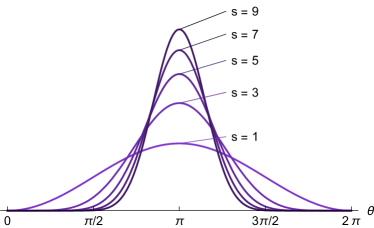
Figure 1: Pulse shape for varying pulse shape parameter $s$. The pulse converges to Dirac delta as $s\rightarrow\infty$.

The case of $M=2$ populations results in eight parameters (excluding the pulse shape parameter $s$). To reduce the problem to a manageable number of parameters, we make the following assumptions: (i) the oscillator properties in populations $\sigma=1,2$ are statistically identical so that $\hat{\eta}_{1}=\hat{\eta}_{2}=:\hat{\eta}$ and $\Delta_{1}=\Delta_{2}=:\Delta$; and (ii) the coupling is symmetric with respect to identical intra- and inter-coupling strengths, i.e., $\kappa_{11}=\kappa_{22}=:\kappa$. and $\kappa_{12}=\kappa_{21}=:a\kappa$. Unless stated otherwise, we keep $(\hat{\eta},\Delta,s)$ fixed and consider $(\kappa,a)$ the main bifurcation parameters.

II.2 Network of Quadratic Integrate and Fire neurons

An equivalent description of the Theta neuron is the quadratic integrate-and-fire (QIF) neuron via the transformation into the membrane potential $V(\theta)=\tan{(\theta/2)}\in(-\infty,\infty)$. The model equations then become BickMartens2020

$$\frac{{\textnormal{d}}}{{\textnormal{d}}t}V_{\sigma,k}:=\dot{V}_{\sigma,k} =V_{\sigma,k}^{2}+\eta_{\sigma,k}+I_{\sigma},\$$ (4)

where $V_{\sigma,k}:=V(\theta_{\sigma,k})$. In this formulation, the neuron fires (emits a spike) when the voltage reaches $V_{k}(t^{-})=\infty$ (in finite time). It is then reset to $V_{k}(t^{+})=-\infty$. QIF neurons have been widely used in neuroscientific modeling; see Ermentrout2010 ; Gerstner2014 for a general introduction and Hansel2001 ; Brunel2003 for a few examples of applications of QIF neurons.

II.3 Exact macroscopic description for the limit of infinitely many neurons

We consider (1) in the limit $N\rightarrow\infty$, which allows us to express the ensemble dynamics in terms of a continuous neuron density $\rho_{\sigma}(\theta,\eta,t)$ governed by the continuity equation

$$\frac{\partial}{\partial t}\rho_{\sigma}+\frac{\partial}{\partial\theta}({f_{\sigma}}\rho_{\sigma}) =0\$$ (5)

where

$$f_{\sigma} =1-\cos\theta+(1+\cos\theta)$$ (6)

$$\times\left(\eta+\sum_{\tau=1}^{M}\kappa_{\sigma\tau}\int_{-\infty}^{\infty}\int_{0}^{2\pi}P_{s}(\theta^{\prime})\rho_{\tau}(\eta^{\prime},\theta^{\prime},t){\textnormal{d}}\theta^{\prime}{\textnormal{d}}\eta^{\prime}\right).\$$

The Ott-Antonsen method OttAntonsen2008 ; Luke2013 facilitates an exact reduction of the microscopic dynamics in (1) to a low-dimensional description of the macroscopic dynamics in terms of the complex order parameter of each population,

$$Z_{\sigma}(t) =R_{\sigma}(t)e^{-i\Phi_{\sigma}(t)}=\int_{0}^{2\pi}\int_{-\infty}^{\infty}e^{i\theta}\rho_{\sigma}(\theta,\eta,t)\,{\textnormal{d}}\eta\,{\textnormal{d}}\theta.\$$ (7)

The absolute value of the order parameter informs us of the level of phase synchronization of the neuron population: when $|Z_{\sigma}|\approx 0$, phases are spread over the circle $\mathbb{T}$, whereas $|Z_{\sigma}|\approx 1$ implies phase synchronization, i.e., phases are closely spread around the phase of the order parameter given by $\Phi_{\sigma}=-\arg{(Z_{\sigma})}$. The collective dynamics of population $\sigma=1,2$ is then given by Luke2013 ; BickMartens2020

$$\begin{split}\dot{Z}_{\sigma}&=-\frac{1}{2}\left[(\Delta_{\sigma}-i\hat{\eta}_{\sigma}-iI_{\sigma}^{(s)})(1+Z_{\sigma})^{2}+i(1-Z_{\sigma})^{2}\right].\ \end{split}$$ (8)

These equations are closed by the input current Luke2013 ; BickMartens2020

$$I_{\sigma}^{(s)} =\sum_{\tau=1}^{M}\kappa_{\sigma\tau}P^{(s)}_{\sigma},$$ (9)

with the average output from all other neurons in the network,

$$P^{(s)}_{\sigma} =a_{s}\left(C_{0}+\sum_{q=1}^{s}C_{q}(Z_{\sigma}^{q}+\bar{Z}_{\sigma}^{q})\right),$$ (10)

$$C_{q} =\sum_{k=0}^{s}\sum_{m=0}^{k}\frac{s!(-1)^{k}\delta_{k-2m,q}}{2^{k}m!(s-k)!(k-m)!}.\$$ (11)

For details on this reduction method and theory in general including applications in neuroscience, see BickMartens2020 .

Two cases are of particular interest to us: pulse shape parameter $s=1$ and $s=\infty$ (impulsive coupling) for which we have

$$P^{(1)}_{\sigma} =1-\frac{1}{2}(Z_{\sigma}+\bar{Z}_{\sigma}),\$$ (12)

and

$$P^{(\infty)}_{\sigma} =\frac{1-|Z_{\sigma}|^{2}}{(1+Z_{\sigma})(1+\bar{Z}_{\sigma})},\$$ (13)

respectively.

II.4 Firing rate equations

The model (8) has an equivalent formulation in terms of average firing rate $r_{\sigma}$ and average membrane potential $v_{\sigma}$ called the Firing Rate Equations (FRE) Montbrio2015 . Indeed, changing variables via the (anti)conformal mapping

$$Z =(1-\bar{W})/(1+\bar{W})\quad\text{or} W =(1-\bar{Z})/(1+\bar{Z}),$$ (14)

gives

$$\dot{W}_{\sigma} =\Delta_{\sigma}+i\hat{\eta}_{\sigma}-iW_{\sigma}^{2}+iI_{\sigma}^{(s)}\$$ (15)

and

$$P^{(1)}_{\sigma} =1-\frac{1-|W_{\sigma}|^{2}}{(1+W_{\sigma})(1+\bar{W_{\sigma}})},\$$ (16)

$$P^{(\infty)}_{\sigma} =\frac{1}{2}(W_{\sigma}+\bar{W}_{\sigma}).$$ (17)

Writing $W_{\sigma}=\pi r_{\sigma}+iv_{\sigma}$, (16) and (17) take the form

$$P^{(1)}_{\sigma} =2\dfrac{\pi^{2}r_{\sigma}^{2}+\pi r_{\sigma}+v^{2}_{\sigma}}{(\pi r_{\sigma}+1)^{2}+v_{\sigma}^{2}},\quad P^{(\infty)}_{\sigma}=\pi r_{\sigma},\$$ (18)

for $s=1$ and $s=\infty$, respectively. Taking real and imaginary part of (15) yields the firing rate equations

$$\dot{r}_{\sigma} =\frac{\Delta_{\sigma}}{\pi}+2r_{\sigma}v_{\sigma},$$ (19)

$$\dot{v}_{\sigma} =v_{\sigma}^{2}-\pi^{2}r_{\sigma}^{2}+\hat{\eta}_{\sigma}+I_{\sigma}^{(s)},\$$ (20)

where

$$I_{\sigma}^{(s)} =\left\{\begin{array}[]{cl}2\sum_{\tau=1}^{M}\kappa_{\sigma\tau}\dfrac{\pi r_{\tau}^{2}+\pi r_{\tau}+v_{\tau}^{2}}{(\pi r_{\tau}+1)^{2}+v_{\tau}^{2}}&,\quad s=1\\ \pi\sum_{\tau=1}^{M}\kappa_{\sigma\tau}r_{\tau}&,\quad s=\infty.\end{array}\right.\$$ (23)

The microscopic and macroscopic description are related as follows. A single Theta neuron fires when its phase crosses $\theta=\pi$; accordingly, the average firing rate $r_{\sigma}(t)$ of the network at time $t$ is defined as the flux through $\theta=\pi$ (or equivalently, the flux at $v_{\sigma}=\infty$), see for instance BickMartens2020 .

III Dynamic behavior of one population

The dynamic behavior for the case of $M=1$ population has already been studied previously Luke2013 ; So2013 . We briefly review the dynamics observed for this case as it is instructive for understanding the dynamic and oscillatory behavior exhibited by $M=2$ populations. For two parameter choices, the model equations (1) for $M=2$ effectively reduce to the dynamics of a single population, $M=1$. Recall that the intra- and inter-coupling strengths among the two populations are given via $\kappa_{11}=\kappa_{22}=\kappa$ and $\kappa_{12}=\kappa_{21}=\kappa a$. Thus, when $a=1$, all neurons experience identical coupling strength so that the two populations act like a single population consisting of twice the number of neurons; on the other hand, when $a=0$, the two populations are decoupled so that each of the two populations in separation effectively corresponds to an $M=1$ system. For brevity, we drop $\sigma$ in (1) and all related equations.

Figure 2: Bifurcation diagrams in $\kappa$ for $M=1$ population of Theta neurons. We display solution branches by reporting maxima and minima in the firing rate $r$ (black) and synchrony level $|Z|$ (gray), respectively. Stable and unstable branches of equilibria have coinciding minima/maxima and are shown solid and dashed, respectively; minima/maxima corresponding to limit cycle behavior are highlighted in blue. Bifurcations that may occur are: saddle node (SN₁, SN₂), Hopf (HB)  and homoclinic (HC). Fixed parameters are $\Delta=0.01$ and pulse shape parameter $s=1$, while $\hat{\eta}=-0.5$ and $\hat{\eta}=0.5$ in panels a) and b), respectively.

The bifurcation diagrams in Fig. 2 report minima and maxima for the firing rate $r$ while varying coupling strength $\kappa$ with parameter values $s=1,\Delta=0.01$ fixed, and $\hat{\eta}=-0.5$ or $\hat{\eta}=0.5$ in panels a) and b), respectively. Solution branches sometimes appear very close to each other for the firing rate $r$, therefore it is instructive to also report the magnitude of the order parameter, $|Z|$, which is related to the firing rate $r$ via the (anti)conformal mapping (14). Equilibria and local bifurcations (saddle-node, Hopf) can be computed analytically from (19) and (20); limit cycles and other bifurcations were computed and continued numerically using Matlab and MatCont software Dhooge2008 , see also Appendix B.

We first consider the case of excitable neurons ($\hat{\eta}<0$) in Fig. 2a). For the parameters considered and $\kappa\lessapprox 0$, we observe a set of stable equilibria (stable nodes) with $|Z|\approx 1$; the related microscopic states are non-oscillatory, i.e., most of the neurons are quiescent (Q), and so their spiking activity is negligible, $r\approx 0$. This branch of equilibria may undergo two saddle-node bifurcations (SN₁  and SN₂) which are connected by a branch of saddles. Equilibria to the right of SN₁  (larger $\kappa$) are stable spirals and correspond to spiking neurons (S) with larger firing rate $r>0$. As the coupling strength $\kappa$ increases, higher levels of synchrony, eventually getting close to $|Z|=1$, may be achieved.

For the case of spiking (firing) neurons ($\hat{\eta}>0$), the bifurcation diagram in Fig. 2b) reveals a similar bifurcation structure with two saddle-node bifurcations. However, for certain values of $\hat{\eta}$, an even more complicated bifurcation scenario is possible along the branch to the right of SN₁: a supercritical Hopf bifurcation (HB) gives birth to limit cycles which ultimately are destroyed in a homoclinic bifurcation (HC). In between the values of $\hat{\eta}=-0.5$ and $\hat{\eta}=0.5$ shown in Fig. 2, two distinct bifurcations of codimension 2 occur: (i) SN₁ and SN₂ merge in a cusp point, and (ii) the bifurcation curves SN₁, HB and HC meet in a Bogdanov-Takens point. The scenario in which limit cycles occur is characteristic for spiking neurons ($\hat{\eta}>0$) with inhibitory coupling ($\kappa<0$), as can be shown by further bifurcation analysis. For further details on these bifurcation structures, see Luke2013 ; So2013 .

Importantly, we note that collective oscillations emerging in the Hopf bifurcation HB cease to exist in the limit of pulses defined by (3) with zero width obtained in the limit of $s\rightarrow\infty$. While this was already noted in recent studies Ratas2016 ; Devalle2017 we briefly outline a derivation of this fact in Appendix A. Further investigations of ours show that Hopf bifurcations continue to exist for a large range of values of the pulse shape parameter, $s$. Our observations suggest that the Hopf bifurcations giving birth to oscillations only vanish in the limit of $s\rightarrow\infty$, prompting a degeneracy for this limit. The case of infinitely narrow pulses, $s=\infty$, provides the advantage that the fixed point conditions resulting from the corresponding FRE can be solved in closed form, enabling a simple mathematical analysis. However, since this case produces a degenerate bifurcation behavior where limit cycles are absent, we chose to fix $s=1$.

Between the pair of fold bifurcations (SN₁ and SN₂) a parameter region of bistability arises, thus facilitating hysteretic behavior. This happens for excitable neurons, $\hat{\eta}<0$, with excitatory coupling, $\kappa>0$, as well as for parameters corresponding to firing neurons, $\hat{\eta}>0$, with inhibitory coupling, $\kappa<0$. This bistable character of solutions observed for $M=1$ population translates to the case of $M=2$ populations, where each population may attain distinct stable configurations.

In the following, we consider non-zero pulse width ($s=1$) and fix parameter values to $\hat{\eta}=-1$ (excitable neurons) and $\Delta=0.01$, while varying the intra-coupling strength, $\kappa$, and the inter-coupling strength, $a$.

IV Analysis for two populations

IV.1 Symmetric and asymmetric equilibria

It is instructive to begin the analysis by surveying the possible asymptotic dynamic behavior for the firing rates $r_{1}$ and $r_{2}$ (or equivalently, $Z_{1}$ and $Z_{2}$) in the FRE (19) and (20) for $M=2$ populations. We may distinguish two types of asymptotic states as $t\rightarrow\infty$, namely (i) symmetric states characterized by $r_{1}(t)=r_{2}(t)$ and $v_{1}(t)=v_{2}(t)$; and (ii) asymmetric states characterized by $r_{1}(t)\neq r_{2}(t)$ and $v_{1}(t)\neq v_{2}(t)$. Furthermore, each neuron population may be in a state of quiescence (Q) or spiking (S), depending on whether $r_{\sigma}$ reflects low or high firing activity, respectively. In an asymmetric limit cycle, both populations oscillate around a distinct value corresponding to quiescence or spiking, respectively. Fig. 3 illustrates the possible asymptotic states that may be observed, depending on parameter values and initial conditions chosen.

Figure 3: Asymptotic dynamic behaviors for the two population model after transients. Low and high levels of the firing rate $r(t)$ indicate quiescent (Q) or spiking (S) behavior. a) Symmetric (stable) equilibrium where both populations are quiescent (QQ). b) Symmetric (stable) equilibrium where both populations are spiking (SS) (Transients leading up to the equilibrium are oscillatory). c) Asymmetric (stable) equilibrium where one population is quiescent and the other spiking (QS  or SQ) (Transients leading up to the equilibrium are oscillatory only for the spiking population). d) Asymmetric (stable) limit cycle (QS${}_{\text{o}}$  or SQ${}_{\text{o}}$) where both populations oscillate with the same period (but with different amplitudes). The coupling parameter is $\kappa=1.8$ for panels a) through c) and $\kappa=2.2$ for panel d); parameters $a=0.25,\hat{\eta}=-1,\Delta=0.01,s=1$ are fixed throughout.

Figure 4: Bifurcation diagrams for $M=2$ populations in $\kappa$ for the firing rate $r_{\sigma}$ reveal symmetric equilibria, $r_{1}=r_{2}$ (black, gray) and asymmetric equilibria, $r_{1}\neq r_{2}$, (red, light red), emerging in bifurcations as follows. a) $a=0$: Both populations are decoupled. Symmetric equilibria are folded in two saddle-node bifurcations (SN₁, SN₂) where the lower and upper branches (black) corresponding to (Q)uiescence and (S)piking, respectively, are stable; the middle branch (gray) is unstable. Thus, four states are possible, (SS, QQ, QS and SQ), facilitating multistability and hysteretic behavior. b) $a=0.18$: Symmetric equilibria with $r_{1}=r_{2}$ seen for $a=0$ are still present (black, gray). However, the unstable branch (gray) undergoes a pitchfork bifurcation in PF₁ and PF₂, giving rise to unstable asymmetric equilibria QS / SQ with $r_{1}\neq r_{2}$ (light red). These equilibria are connected in a loop, folded twice in two saddle-node bifurcations (SN₃ and SN₄), giving rise to the co-existence of two stable asymmetric states (red) where one population is quiescent while the other is spiking, (SQ or QS). c) $a=-0.01$: For $a<0$ the order of SN₃, SN₄ and SN₁, SN₂, PF₁, PF₂ is reversed along the $\kappa$ direction when compared to $a>0$. Parameters are $\Delta=0.01,\hat{\eta}=-1,s=1$ everywhere. Chosen values for $a$ are indicated as dashed horizontal lines in Fig. 6.

Solution branches reported in Fig. 2 for $M=1$ population translate to symmetric states in the model with $M=2$ populations. To see this, let us first consider two special parameter choices: $a=0$ (decoupled populations) and $a=1$ (two populations effectively act like one large population). In these cases, the system with $M=2$ populations displays the same bifurcation behavior as $M=1$ population, as shown in Fig. 4a) for $a=0$. The branch with low firing rate (QQ) corresponds to quiescent neurons with coherent stationary phases; whereas the branch with high firing rate (SS) corresponds to spiking populations whose synchronization level and firing rate grow with increasing coupling strength $\kappa$. Just as for $M=1$ population, the system exhibits bistable regions in which both configurations, (Q)uiescence and (S)piking, are possible. However, note that in the case of $a=1$, both populations may only attain identical (symmetric) configurations of quiescence or spiking, namely SS or QQ; in contrast, the decoupled case with $a=0$ additionally and trivially allows for the two populations to attain distinct (asymmetric) configurations, namely, SQ or QS. Importantly, symmetric states persist even when $a\neq 0$ or $a\neq 1$ since parameters are symmetric across the two populations. Specifically, if $r$ is an equilibrium of the $M=1$ population system, then so is $(r,r)$ an equilibrium of the $M=2$ population system but now with $\kappa$ replaced by $\kappa/(1+a)$. For this reason, the solution branches of symmetric equilibria seen for $M=1$ translate to the $M=2$ system, including the saddle-node bifurcations SN₁ and SN₂ seen in Fig. 2, in between which, for $a\geq 0$, two stable symmetric states SS and QQ co-exist. However, for $a<0$, the region of bistability for symmetric states is bounded by the pitchfork bifurcations PF₁ and PF₂ rather than SN₁ and SN₂, since both branches emanating from the bifurcation point SN₁ (SN₂) are unstable, one of them gaining stability at PF₁ (PF₂), see Figs. 4c) and 6a). PF₁ and PF₂ also give rise to asymmetric states, as we explain in the following.

Asymmetric states, corresponding to QS or SQ configurations with $r_{1}\neq r_{2}$, are trivially possible when the two populations are decoupled ($a=0$); however, their range of existence and stability off the degenerate cases $a\neq 0$ and $a\neq 1$ deserves further exploration, and we consider small perturbations for $a\neq 0$. Considering the case of $a=0.18$ in Fig. 4b) we observe that unstable asymmetric states (light red) branch off the unstable symmetric state (gray) in pitchfork bifurcations PF₁ and PF₂  (see also inset). The set of asymmetric equilibria forms a loop in $(\kappa,r)$-space with two folds, i.e., the equilibria undergo saddle-node bifurcations in SN₃ and SN₄, between which asymmetric states are stable. As a result, the QS and SQ (red) emerge as bistable asymmetric configurations. These stable asymmetric branches may co-exist with the bistable symmetric solution branches QQ and SS  (black). Note that for $a>0$, PF₁ and PF₂ lie outside SN₃ and SN₄, while for $a<0$ PF₁ and PF₂ lie inside SN₃ and SN₄; as a consequence, the existence of asymmetric states is bounded by PF₁ and PF₂ for $a>0$ and SN₃ and SN₄ for $a<0$, see Fig. 4b) and c). Moreover, for $a>0$, asymmetric states exist only in a relatively narrow range of intermediate coupling strength $\kappa$; by contrast, for $a\leq 0$, the $\kappa-$range of existence of asymmetric equilibria rapidly expands as the value of $a$ decreases (see Fig. 6a).

Note that, considering the case of decoupled populations with $a=0$, symmetric and asymmetric branches may appear like they coincide when inspecting Fig. 4, however, the two types of solution branches are not identical: While the projections $Z_{1}\in\mathbb{C}$ and $Z_{2}\in\mathbb{C}$ indeed share identical values for symmetric and asymmetric equilibria, this cannot hold true in the full phase space for $(Z_{1},Z_{2})\in\mathbb{C}^{2}$, where the definitions for symmetric ($r_{1}=r_{2},v_{1}=v_{2}$) and asymmetric states ($r_{1}\neq r_{2},v_{1}\neq v_{2}$) are obeyed.

IV.2 Birth and destruction of limit cycle oscillations

Figure 5: Birth and destruction of asymmetric limit cycle oscillations (blue) in the firing rate for $M=2$ populations while varying $\kappa$. Possible bifurcation scenarios are illustrated for various values of $a$ (also indicated as dashed lines in Fig. 6). a) $a=0.204$: stable limit cycles are born in the supercritical Hopf bifurcation HB_-(the bifurcation curve is intersected twice, see Fig. 6). b) $a=0.25$: stable and unstable limit cycles are born in HB_- and HB_+-, respectively, and annihilate in a saddle-node of limit cycles bifurcation (SNLC₁). c) $a=0.297$: stable and unstable limit cycles are destroyed in a homoclinic bifurcation HC_- and HC₊, respectively. Moreover, the unstable cycle is subject to two saddle-node-of-limit-cycles bifurcations at SNLC₁ and SNLC₂, in between which it gains stability (see inset); the unstable limit cycle branch emerging from SNLC₂ gets destroyed in HC₊. d) $a=0.302$: the unstable limit cycle born in HB_+- is destroyed in the homoclinic HC₊ ; saddle-node-of-limit-cycles bifurcations are now absent. Symmetric equilibria connecting to PF₁  and PF₂  are omitted for simplicity. Stable and unstable solution branches are shown as dark and light colored shades, respectively. Parameters are $\Delta=0.01,\hat{\eta}=-1,s=1$ everywhere.

For larger values of the inter-coupling strength, $a$, asymmetric equilibria QS (SQ) may undergo Hopf bifurcations giving rise to limit cycle oscillations (QS${}_{\text{o}}$, SQ${}_{\text{o}}$), indicated by their minima/maxima (blue) in Fig. 5a) through d). Since these limit cycles branch off asymmetric equilibria (red), they correspond to asymmetric configurations characterized by firing rates $r_{1}(t)\neq r_{2}(t)$. These limit cycles are created and destroyed in various bifurcations, as outlined in the following.

Birth of stable limit cycles (HB_-).

Stable limit cycles (blue minima/maxima) are born in the supercritical Hopf bifurcation denoted by HB_-, as shown in Fig. 5a) for $a=0.204$. As $\kappa$ increases, the amplitude waxes and wanes, as the bifurcation HB_- is intersected twice in the direction of varying $\kappa$, see also Fig. 6).

Birth of stable/unstable limit cycles and annihilation in saddle-node-of-limit-cycle bifurcation (HB_-,HB_+-,SNLC₁).

Stable limit cycles (blue) are still born in a supercritical Hopf bifurcation at HB_-, but now an unstable limit cycle (light blue) of smaller amplitude emerges for greater $\kappa$ in the supercritical Hopf (with repelling center manifold) at HB_+-. The continuum of cycles folds over in a saddle-node of limit cycles bifurcation at SNLC₁, where the stable and unstable limit cycles coalesce and disappear, see Fig. 5b) for $a=0.25$.

Stabilization of unstable limit cycle in secondary saddle-node-of-limit-cycle bifurcation (SNLC₂).

Stable and unstable limit cycles are created in HB_- and HB_+-. While the stable limit cycle is destroyed in the homoclinic bifurcation HC_-, the unstable limit cycle is subject to a more complicated series of bifurcations: It undergoes not only one, but two saddle-node of cycles bifurcations, SNLC₂ and SNLC₁. The unstable limit cycle emerging from SNLC₂ collides with the saddle equilibrium of the asymmetric branch in the homoclinic bifurcation HC₊ and is destroyed, as shown in Fig. 5c) for $a=0.297$.

Simple birth and destruction of stable/unstable limit cycles (HB_-, HC_-, HB_+-, HC₊).

The stable and unstable limit cycles are born in the Hopf bifurcations HB_- and HB_+- and are destroyed in the homoclinic bifurcations HC_- and HC₊, respectively. The complicated scenario including two saddle-node-of-limit-cycles bifurcations from IV.2 is entirely absent. This simple scenario is shown in Fig. 5d) for $a=0.302$.

IV.3 Stability diagram

We now explain how the various bifurcation scenarios are related, i.e., how stability boundaries are connected in the $(\kappa,a)$-parameter plane and how bifurcation curves are structured around bifurcation points of higher co-dimension.

Let us first consider the overall bifurcation structure for a larger parameter range ($\kappa,a$) as displayed in Fig. 6a), mainly focusing on symmetric (QQ, SS) and asymmetric equilibria QS (or SQ). On the branches of symmetric equilibria (QQ, SS) two saddle-node bifurcations occur, SN₁  and SN₂ (black), which coalesce in a codimension 2 cusp point for large $a$ (not shown). The gray shaded region of bistability between QQ and SS is bounded by SN₁ and SN₂ for $a\geq 0$ and by PF₁ and PF₂ (dashed black curves in Fig. 6a)) for $a<0$, respectively. Note that the curve PF₂ lies very close to SN₂ in the shown parameter range, $-0.4\leq a\leq 0.7$.

Unstable saddle branches of the symmetric equilibria between (or outside) SN₁ and SN₂  undergo pitchfork bifurcations PF₁ and PF₂, which give rise to unstable asymmetric branches (see light red curves in Fig. 4b) and c) and Fig. 5a) through d)). These unstable asymmetric branches gain stability on the saddle-node bifurcation curves SN₃ and SN₄ (red curves in Fig. 6a)), which meet in the codimension 2 cusp point CP. The resulting asymmetric stable configurations (QS or SQ) reside inside the red shaded region bounded by the saddle-node bifurcation curves SN₃ and SN₄ and the supercritical Hopf bifurcation curves HB_- and HB’.

In HB_- and HB’, stable asymmetric equilibria QS and SQ lose stability, resulting in stable asymmetric limit cycles QS${}_{\text{o}}$ (or SQ${}_{\text{o}}$) within the blue shaded regions; these limit cycles may get destroyed in the homoclinic bifurcations denoted by HC_- and HC’ (violet). Hopf (HB_- and HB’) and homoclinic bifurcation curves associated with the emergence and destruction of these limit cycles (HC_- and HC’) meet with the (asymmetric) saddle-node bifurcation curve SN₃ in two other bifurcation points of codimension 2, namely the Bogdanov-Takens points BT and BT’, respectively, characterized by double zero eigenvalues Kuznetsov1998 .

Figure 6: Stability diagram for $M=2$ populations in the $(\kappa,a)$-parameter plane with $\Delta=0.01,\hat{\eta}=-1,s=1$ fixed. Gray shading indicates a bistable region of the two stable symmetric equilibria, QQ and SS. Red shading indicates the bistable region of stable asymmetric equilibria, that is, QS, or, equivalently, SQ. Blue shading indicates the bistable region of stable asymmetric limit cycles (QS${}_{\text{o}}$ and SQ${}_{\text{o}}$). Dashed black lines delineate the choices of parameter $a$ for the bifurcation diagrams in Fig. 4 and Fig. 5.

The bifurcations pertaining to the asymmetric limit cycles are structured around further, more complicated bifurcation curves and bifurcation points of higher co-dimension, see Fig. 6b) and c). Following the Hopf bifurcation curve HB_- in panel b), we arrive at a Generalized Hopf bifurcation point (GH) of codimension 2 Kuznetsov1998 ; Guckenheimer2007GH . Such a point not only has a pair of purely imaginary eigenvalues, but also the first Lyapunov coefficient for the Hopf bifurcation changes sign at this point so that subcritical (HB₊) and supercritical (HB_-) Hopf bifurcations are separated in GH; in addition, a branch of saddle-node of limit cycle bifurcations, SNLC₁, emerges from GH where the stable and unstable limit cycles born in HB_- and HB₊ are annihilated.

Following the bifurcation curve HB₊, the associated subcritical Hopf bifurcation tangentially intersects the saddle-node bifurcation SN₄ in the Zero-Hopf bifurcation ZH (or saddle-node Hopf bifurcation) Kuznetsov1998 ; Guckenheimer2007ZH , characterized by a zero eigenvalue and a pair of purely imaginary eigenvalues. At ZH, the first Lyapunov coefficient vanishes once more and changes sign. Hopf bifurcations HB_+- above the ZH point are supercritical (i.e., having a negative first Lyapunov coefficient), but continue to produce unstable limit cycles as the center manifold (of the Hopf bifurcation) is repelling.

Following the saddle-node bifurcation of limit cycles curve SNLC₁, we observe that it terminates in another bifurcation point of codimension 2, Cusp of Cycles (CPC), where it collides with a second saddle-node bifurcation of limit cycles curve SNLC₂. This latter bifurcation curve merges with the homoclinic bifurcation curve HC₊ in a codimension $\geq 2$ point SLH, see Fig. 6c). The point SLH separates two branches of the homoclinic curves, HC_- and HC₊, and tangentially intersects with SNLC₂. Homoclinic bifurcations on HC_- (HC₊) destroy stable (unstable) limit cycles as $\kappa$ approaches the homoclinic bifurcation point from above (below).

We come to the following conclusion. In similarity with the case of $M=1$ population, the cases of very small and very strong coupling $\kappa$ result in regimes with quiescent and spiking activity, respectively; both are characterized by high levels of synchrony. In the intermediate regime, the dynamic behavior is more complicated. We thus find the following five stability regions: (i) for small coupling strength $\kappa$, both populations are quiescent, corresponding to the symmetric configuration QQ (white region); (ii) for large coupling strength $\kappa$, both populations are spiking, corresponding to the symmetric configuration SS (white region); (iii) for intermediate coupling strengths, we find a region of bistability between the configurations QQ and SS (gray region); this region of bistability co-exists with asymmetric configurations of either (iv) stationary firing rate, SQ or QS (red region), or (v) oscillatory firing rates, SQ${}_{\text{o}}$ or QS${}_{\text{o}}$ (blue region). In addition, there are regions for intermediate coupling strengths where only QQ co-exists stably with SQ and QS; or only SS with SQ and QS (see Fig. 6a)).

V Discussion

Collective oscillations in neural ensembles are responsible for the rhythm generation required for solving functionally relevant tasks in the brain Buzsaki2012 ; Uhlhaas2006 ; Marder2001 . Collective oscillations may be facilitated by a variety of network setups, including heterogeneous networks with excitatory and inhibitory coupling leading to gamma rhythms Keeley2019 ; Segneri2020 . Here, we investigated the emergence of collective oscillations in a simple model consisting of a homogeneous network composed of two (statistically) identical populations of type 1 neurons with non-uniform but symmetric coupling, i.e., neurons are coupled with strength $\kappa$ and $a\kappa$ (with $a\neq 1$) within and between the two populations, respectively.

In this model, each population may assume states corresponding to quiescent (Q) or spiking (S) firing activity. Thus, we may distinguish symmetric configurations, where both populations are either quiescent or spiking (QQ, SS), and asymmetric configurations, where one population is quiescent but the other is spiking (SQ, QS). We found that stable symmetric configurations may co-exist for certain parameter choices (see Fig. 4a)). We did not find that symmetric configurations are oscillatory except for uniform coupling ($a=1$) or for absent inter-coupling ($a=0$). As we deviate from uniform coupling, $a\neq 1$, unstable asymmetric equilibria emerge from symmetric configurations in symmetry-breaking pitchfork bifurcations. Along these solution branches, asymmetric equilibria may further undergo saddle-node bifurcations and thus gain stability (see Fig. 4b)). Asymmetric oscillatory configurations (QS${}_{\text{o}}$, SQ${}_{\text{o}}$) emerge in Hopf bifurcations (Fig. 5) that are organized around higher codimension bifurcation points. Depending on parameters, symmetric and asymmetric configurations may be stable and co-exist, resulting in multistability between either stationary configurations only (QQ, SS, QS, SQ); or between stationary and oscillatory configurations (QQ, SS, QS${}_{\text{o}}$, SQ${}_{\text{o}}$). For these regions of stability we have determined valid parameter regions and stability boundaries (Fig. 6).

Oscillator networks with such modular network structure are known to exhibit a high degree of multistability, i.e., depending on initial conditions, a variety of dynamic configurations for the collective states may be assumed in each population. A prominent example are synchronization patterns known as chimera states in Kuramoto oscillator networks Abrams2008 ; Martens2010bistable ; PanaggioAbramsReview2015 , which may be employed to store memory or perform computations BickMartens2015 or direct the flow of information between populations DeschleDaffertshoferBattagliaMartens2019 ; BickMartens2020 . However, compared to Kuramoto networks with rigidly rotating oscillators, the excitable nature of neurons intrinsically leads to more complicated dynamics and synchronization behavior Calugaru2019 . While complicated dynamics may arise in networks composed of identical Kuramoto oscillators arranged with at least two populations (as well as for broken parameter symmetries) MartensPanaggioAbrams2016 ; Bick2018 , excitable type 1 neurons produce rich bifurcation behavior and bistability already for a single population, as illustrated in Fig. 4 and discussed in Luke2013 ; BickMartens2020 . Such multistability is of great interest in applications, e.g. in neuroscience. A recent study modeled networks of type 1 neurons and demonstrated how the bistability between low and high firing activity — resulting in a large configuration space that scales with the number of populations — may be employed to solve cognitive tasks such as memory storage and recall Schmidt2018 .

Several studies considered networks of type 1 neurons in terms of their macroscopic behavior. The collective dynamics of a single population was studied in terms of non-identical Theta neurons with non-zero pulse width Luke2013 ; So2013 , of the response to an external (rigid) forcing Luke2014 , of quadratic integrate-and-fire neurons Montbrio2015 , and of different coupling functions, oscillations and aging transitions Ratas2016 , and of the role of distributed delay in the coupling function Ratas2018 . Luke et al Luke2014 studied a two population model similar to ours; however, they considered unidirectional coupling. This driver-response system exhibits some of the bifurcation structures and collective macroscopic behaviors that we reported here: i.e., the response population exhibits multistable equilibrium states and limit cycles. In addition, their system exhibits chaotic behavior, which was also reported by Ceni et al. Ceni2020 who considered a similar setup, but with exponentially decaying synapses leading to three dimensional dynamics for the macroscopic firing rate equations. Unlike their study, we did not observe quasiperiodic and chaotic dynamics. While we restricted our study to symmetric parameter configurations between the two populations, future research might address the question if breaking parameter symmetries between the populations (such as the coupling strength) may induce bifurcations leading to chaos. For such cases, one may envision torus bifurcations emerging from the Zero-Hopf bifurcations Kuznetsov1998 , offering a route to chaos via bifurcations of Shil’nikov homoclinic orbits to saddle foci. Ratas and Pyragas Ratas2017 studied a network of quadratic integrate-and-fire neurons with two populations. While their system is similar to ours, it differs in some important aspects. Firstly, neurons are considered to be strongly heterogeneous with an excitability spread around $\hat{\eta}=0$, thus resulting in a network including both excitable and spiking neurons; here, the majority of neurons are excitable. Secondly, for the coupling function, they use a threshold modulation coupling function corresponding to a Heaviside function. This system exhibits steady and oscillatory states with symmetric and asymmetric character, but unlike our system, also chaotic behavior and states characterized by anti-phase configurations.

To study collective oscillations of firing activity in our model, it is necessary to deviate from the case of instantaneous pulse coupling ($s\rightarrow\infty$) where collective oscillations are absent (see Appendix A and Ratas2016 ; Devalle2017 ). The pulse width given by Eq. (3) with $s=1$ was large; other pulse shape models Montbrio2015 ; Gerstner2014 may be more realistic and consider that incident pulses arrive instantaneously in order to decay exponentially fast upon arrival over a characteristic time scale $\tau$. It is then frequently assumed that $\tau\rightarrow 0$, resulting in time-symmetric and instantaneous pulses. This strategy certainly simplifies analysis; yet, it appears that this limit biophysically is no more realistic, especially since it results in the same macroscopic equations as given by (19) and (20) for the limit of $s\rightarrow\infty$; this again rules out the potential to produce any macroscopic oscillations. For a future study it might be interesting to examine how the specific choice of pulse shape in terms of width and time-asymmetry affects the unfolding of bifurcations. While many studies either studied small values of $s$ or $s\rightarrow\infty$, it would be interesting to see how the bifurcation scenarios reported in this study translate to the case of causal synaptic potentials that decay exponentially in time  Coombes2019next .

Many questions remain. For instance, breaking parameter symmetry may result in richer dynamics Martens2016 including chaos Bick2018 ; is chaotic motion feasible if excitability parameters ($\hat{\eta}_{\sigma}$ and $\Delta_{\sigma}$) are non-identical, or if small delay is introduced in the coupling? Are bifurcation scenarios for spiking neurons ($\hat{\eta}>0$) equally complicated as the ones we observed here for excitable neurons ($\hat{\eta}<0$)? In terms of switching between configurations and devising a control method to do this, it may be useful to determine basins of attraction for the various configurations or responses to directed perturbations MartensPanaggioAbrams2016 ; Schmidt2018 . Furthermore, networks with larger population number $M>2$ provide a larger set of dynamic configurations Shanahan2010 ; Wildie2012 ; Schmidt2018 ; but how large is the set of configurations as a function of the population number, and which of the configurations are stable, and which oscillatory? Future studies may address such and further questions.

AIP Data Sharing Policy

Data sharing is not applicable to this article as no new data were created or analyzed in this study.

Appendix A Collective oscillations for non-zero pulse width ($s<\infty$)

We briefly discuss the existence of Hopf bifurcations and resulting limit cycle oscillations in the firing rate $r(t)$ for varying pulse shape parameter $s$, for the simple case of $M=1$ population. To determine the presence of Hopf instabilities, we examine eigenvalues of the Jacobian of (19),

$$J =\left(\begin{array}[]{cc}2v&2r\\ -2\pi^{2}r+\frac{\partial}{\partial r}I&2v+\frac{\partial}{\partial v}I\end{array}\right).\$$ (26)

Steady state of (19) implies $v^{*}=-\frac{\Delta}{2\pi}\frac{1}{r^{*}}$ so that

$$\text{tr}{(J)} =-\frac{2\Delta}{\pi}\frac{1}{r^{*}}+\frac{\partial}{\partial v}I|_{(r,v)=(r^{*},v^{*})}.\$$ (27)

A necessary condition for a Hopf bifurcation is that $\text{tr}{(J)}=0$. For the case of infinitely narrow pulses, $s=\infty$, Hopf bifurcations are impossible: we have $\frac{\partial}{\partial v}I=\kappa\frac{\partial}{\partial v}P^{(\infty)}=0$ and thus $\text{tr}{(J)}=-2\Delta/\pi/r^{*}<0$ for all $r^{*}>0$. Hence, Hopf bifurcations and resulting limit cycles regardless of the choice of parameters can be ruled out for this case.

Conversely, we know that Hopf bifurcations are possible for $s=1$ (see Fig. 2) and $s=2$ (see Luke et al. Luke2013 ). Indeed, the trace for $1<s<\infty$ involves more complicated terms, and Hopf bifurcation cannot easily be ruled out. While an analytical proof remains elusive, using a numerical analysis based on solving the zero trace condition, one finds that limit cycle oscillations are feasible for a large range of pulse shape parameters, including at least $1\leq s\leq 20$.

Appendix B Methodology

The data for the bifurcation diagrams in Figs. 4 and 5 was obtained via numerical continuation of equilibria and limit cycles (using MatCont software) in the parameter $\kappa$; thus we encountered codimension-1 bifurcation points SN₁, SN₂, SN₃, SN₄, HB_-, HB₊, HB_+-, HB’, HC_-, HC₊, HC’, SNLC₁, SNLC₂, PF₁, PF₂. With the exception of PF₁ and PF₂ we continued all these degenerate states as bifurcation curves in the parameters $\kappa$ and $a$ using MatCont (Fig. 6); thereby we detected the codimension $\geq 2$ bifurcation points reported in Sec. IV 3. The direct two-parameter continuation of the bifurcation curves PF₁, PF₂  posed technical problems when using MatCont; instead we therefore determined the loci of PF₁ and PF₂ by computing bifurcation diagrams in a single parameter, $\kappa$, for set values of $a$, resulting in the parameter list $(\kappa,a)$ in Tab. 1. The curves shown in Fig. 6 (dashed black curves) are splines interpolating these data points.

$a$	$\kappa$ (PF1)	$\kappa$ (PF2)
0.7	1.476	5.546
0.65	1.438	5.728
0.6	1.414	5.915
0.5	1.400	6.320
0.4	1.419	6.777
0.35	1.439	7.029
0.25	1.500	7.594
0.204	1.538	7.884
0.18	1.561	8.045
0.1	1.652	8.630
-0.01	1.824	9.590
-0.05	1.904	9.993
-0.1	2.020	10.548
-0.15	2.160	11.169
-0.2	2.329	11.867
-0.27	2.632	13.004
-0.35	3.117	14.604
-0.4	3.538	15.821

Table 1: Bifurcation points numerically detected for PF₁ and PF₂.

References

- [1] G. B. Ermentrout and N. Kopell. Parabolic Bursting in an excitable system coupled with a slow oscillation. SIAM Journal on Applied Mathematics, 46(2):233–253, 1986.
- [2] P. E. Latham, B. J. Richmond, P. G. Nelson, and S. Nirenberg. Intrinsic dynamics in neuronal networks. I. Theory. Journal of Neurophysiology, 83(2):808–827, 2000.
- [3] D. Hansel and G. Mato. Existence and stability of persistent states in large neuronal networks. Physical Review Letters, 86(18):4175–4178, 2001.
- [4] W. Gerstner, W. M. Kistler, R. Naud, and L. Paninski. Neuronal dynamics: From single neurons to networks and models of cognition. Cambridge University Press, 2014.
- [5] E. Ott and T. M. Antonsen. Low dimensional behavior of large systems of globally coupled oscillators. Chaos (Woodbury, N.Y.), 18(3):037113, sep 2008.
- [6] E. Montbrió, D. Pazó, and A. Roxin. Macroscopic description for networks of spiking neurons. Physical Review X, 5(2):1–15, 2015.
- [7] T. B. Luke, E. Barreto, and P. So. Complete Classification of the Macroscopic Behavior of a Heterogeneous Network of Theta Neurons. Neural Computation, 25:3207–3234, 2013.
- [8] C. Bick, C. Laing, M. Goodfellow, and E.A. Martens. Understanding the dynamics of biological and neural oscillator networks through exact mean-field reductions: a review. Journal of Mathematical Neuroscience, 9(10), 2020.
- [9] Á. Byrne, D. Avitabile, and S. Coombes. Next-generation neural field model: The evolution of synchrony within patterns and waves. Physical Review E, 2019.
- [10] E. Marder and D. Bucher. Central pattern generators and the control of rythmic movements. Current Biology, 11:R986–R996, 2001.
- [11] J. C. Smith, H. H. Ellenberger, K. Ballanyi, D. W. Richter, and J. L. Feldman. Pre-Bötzinger Complex: A Brainstem Region That May Generate Respiratory Rhythm in Mammals. Science, 254(5032):726–729, 1991.
- [12] G. Buzsáki and X.-J. Wang. Mechanisms of Gamma Oscillations. Annual Review of Neuroscience, 35(1):203–225, 2012.
- [13] E. T. Bullmore and O. Sporns. Complex brain networks: graph theoretical analysis of structural and functional systems. Nature reviews. Neuroscience, 10(3):186–98, 2009.
- [14] D. Meunier, R. Lambiotte, and E. T. Bullmore. Modular and hierarchically modular organization of brain networks. Frontiers in Neuroscience, 4(DEC):1–11, 2010.
- [15] K. D. Harris. Neural signatures of cell assembly organization : Article : Nature Reviews Neuroscience. Nature Reviews, 6(May):399–407, 2005.
- [16] C. W. Lynn and D. S. Bassett. The physics of brain network structure, function and control. Nature Reviews Physics, 2019.
- [17] L. Glass. Synchronization and rhythmic processes in physiology. Nature, 410(March):277–284, 2001.
- [18] P. J. Uhlhaas and W. Singer. Neural synchrony in brain disorders: relevance for cognitive dysfunctions and pathophysiology. Neuron, 52(1):155–68, 2006.
- [19] J. Fell and N. Axmacher. The role of phase synchronization in memory processes. Nature Reviews Neuroscience, 12(2):105–118, 2011.
- [20] P. Fries. Neuronal gamma-band synchronization as a fundamental process in cortical computation. Annual Review of Neuroscience, 32:209–24, 2009.
- [21] X. J. Wang. Neurophysiological and Computational Principles of Cortical Rhythms in Cognition. Physiological Reviews, 90(3):1195–1268, 2010.
- [22] W. Singer and C. M. Gray. Visual feature integration and the temporal correlation hypothesis. Ann Rev Neurosci, 18:555–586, 1995.
- [23] P. Fries. A mechanism for cognitive dynamics: neuronal communication through neuronal coherence. Trends in Cognitive Sciences, 9(10):474–80, 2005.
- [24] M. I. Rabinovich, V. S. Afraimovich, C. Bick, and P. Varona. Information flow dynamics in the brain. Physics of Life Reviews, 9(1):51–73, 2012.
- [25] C. Kirst, M. Timme, and D. Battaglia. Dynamic information routing in complex networks. Nature Communications, 7:11061, 2016.
- [26] N. Deschle, A. Daffertshofer, D. Battaglia, and E.A. Martens. Directed Flow of Information in Chimera States. Frontiers in Applied Mathematics and Statistics, 5(28), 2019.
- [27] D. M. Abrams, R. Mirollo, S. H. Strogatz, and D. A. Wiley. Solvable model for chimera states of coupled oscillators. Phys. Rev. Lett, 101:084103, 2008.
- [28] E. A. Martens, M. J. Panaggio, and D. M. Abrams. Basins of Attraction for Chimera States. New Journal of Physics, Fast Track Communication, 18:022002, 2016.
- [29] E. A. Martens. Bistable Chimera Attractors on a Triangular Network of Oscillator Populations. Physical Review E, 82(1):016216, jul 2010.
- [30] E. A. Martens, C. Bick, and M. J. Panaggio. Chimera states in two populations with heterogeneous phase-lag. Chaos, 26(9):094819, 2016.
- [31] C. R. Laing. The dynamics of chimera states in heterogeneous Kuramoto networks. Physica D: Nonlinear Phenomena, 238(16):1569–1588, aug 2009.
- [32] C. R. Laing, K. Rajendran, and I. G. Kevrekidis. Chimeras in random non-complete networks of phase oscillators. Chaos: An Interdisciplinary Journal of Nonlinear Science, 22(1):013132, 2012.
- [33] E. Schöll. Synchronization patterns and chimera states in complex networks: Interplay of topology and dynamics. The European Physical Journal Special Topics, 225(6-7):891–919, 2016.
- [34] M. J. Panaggio and D. M. Abrams. Chimera states: coexistence of coherence and incoherence in networks of coupled oscillators. Nonlinearity, 28(3):R67, 2015.
- [35] C. R. Laing. Phase oscillator network models of brain dynamics. In Ahmed A. Moustafa, editor, Computational Models of Brain and Behavior, chapter 37, pages 505–518. Wiley-Blackwell, 2017.
- [36] T. B. Luke, E. Barreto, and P. So. Macroscopic complexity from an autonomous network of networks of theta neurons. Frontiers in Computational Neuroscience, 8(NOV):1–11, 2014.
- [37] H. Schmidt, D. Avitabile, E. Montbrió, and A. Roxin. Network mechanisms underlying the role of oscillations in cognitive tasks. PLoS Computational Biology, 14(9):1–24, 2018.
- [38] M. Yamakou, P. G. Hjorth, and E. A. Martens. Optimal self-induced stochastic resonance in multiplex neural networks: electrical versus chemical synapses. Frontiers in Neuroscience, 14(62), 2020.
- [39] G. Weerasinghe, B. Duchet, H. Cagnan, P.r Brown, C. Bick, and R. Bogacz. Predicting the effects of deep brain stimulation using a reduced coupled oscillator model. PLoS Comp. Biology, 15(8), 2018.
- [40] S. Watanabe and S. H. Strogatz. Constants of motion for superconducting Josephson arrays. Physica D, 74(3-4):197–253, 1994.
- [41] C. R. Laing. The Dynamics of Networks of Identical Theta Neurons. Journal of Mathematical Neuroscience, 8(1), 2018.
- [42] H. R. Wilson and J. D. Cowan. Excitatory and inhibitory interactions in localized populations of model neurons. Biophysical journal, 12(1):1–24, 1972.
- [43] S. Amari. Dynamics of pattern formation in lateral-inhibition type neural fields. Biological Cybernetics, 27(2):77–87, 1977.
- [44] L. Lin, E. Barreto, and P. So. Synaptic Diversity Suppresses Complex Collective Behavior in Networks of Theta Neurons. Frontiers in Computational Neuroscience, 14(May):1–17, 2020.
- [45] G. Buzsáki and B. O. Watson. Brain rhythms and neural syntax: Implications for efficient coding of cognitive content and neuropsychiatric disease. Dialogues in Clinical Neuroscience, 2012.
- [46] P. Fries, D. Nikolić, and W. Singer. The gamma cycle. Trends in neurosciences, 30(7):309–316, 2007.
- [47] S. Keeley, A. Fenton, and J. Rinzel. Modeling fast and slow gamma oscillations with interneurons of different subtype. Journal of Neurophysiology, 117(3):950–965, 2017.
- [48] S. Keeley, A. Byrne, A. Fenton, and J. Rinzel. Firing rate models for gamma oscillations. Journal of Neurophysiology, 121(6):2181–2190, 2019.
- [49] M. Segneri, H. Bi, S. Olmi, and A. Torcini. Theta-nested gamma oscillations in next generation neural mass models. Frontiers in Computational Neuroscience, pages 1–28, 2020.
- [50] F. Devalle, A. Roxin, and E. Montbrió. Firing rate equations require a spike synchrony mechanism to correctly describe fast oscillations in inhibitory networks. PLoS Computational Biology, 13(12):1–21, 2017.
- [51] P. So, T. B. Luke, and E. Barreto. Networks of theta neurons with time-varying excitability: Macroscopic chaos, multistability, and final-state uncertainty. Physica D: Nonlinear Phenomena, 267:16–26, may 2013.
- [52] A. Dhooge, W. Govaerts, Yu A. Kuznetsov, H. G.E. Meijer, and B. Sautois. New features of the software MatCont for bifurcation analysis of dynamical systems. Mathematical and Computer Modelling of Dynamical Systems, 2008.
- [53] B. Ermentrout. Ermentrout-Kopell canonical model. Scholarpedia, 3(3):1398, 2008.
- [54] J. T. Ariaratnam and S. H. Strogatz. Phase diagram for the Winfree model of coupled nonlinear oscillators. Physical Review Letters, 86(19):4278, 2001.
- [55] G. B. Ermentrout and D. H. Terman. Mathematical Foundations of Neuroscience, volume 35 of Interdisciplinary Applied Mathematics. Springer, New York, NY, 2010.
- [56] N. Brunel and P. E. Latham. Firing rate of the noisy quadratic integrate-and-fire neuron. Neural Computation, 15(10):2281–2306, 2003.
- [57] I. Ratas and K. Pyragas. Macroscopic self-oscillations and aging transition in a network of synaptically coupled quadratic integrate-and-fire neurons. Physical Review E, 94(3):1–11, 2016.
- [58] Y. A. Kuznetsov. Elements of applied bifurcation theory. Springer-Verlag, New York, 1998.
- [59] J. Guckenheimer and Y. Kuznetsov. Bautin bifurcation. Scholarpedia, 2007.
- [60] J. Guckenheimer and Y. Kuznetsov. Fold-Hopf bifurcation. Scholarpedia, 2007.
- [61] C. Bick and E. A. Martens. Controlling Chimeras. New Journal of Physics, 17:033030, 2015.
- [62] D. Călugăru, J. F. Totz, E. A. Martens, and H. Engel. First-order synchronization transition in a large population of strongly coupled relaxation oscillators. Science Advances, 6(39):eabb2637, 2020.
- [63] C. Bick, M. J. Panaggio, and E. A. Martens. Chaos in Kuramoto Oscillator Networks. Chaos, 28:071102, 2018.
- [64] I. Ratas and K. Pyragas. Macroscopic oscillations of a quadratic integrate-and-fire neuron network with global distributed-delay coupling. Physical Review E, 98(5):1–11, 2018.
- [65] A. Ceni, S. Olmi, A. Torcini, and D. Angulo-Garcia. Cross frequency coupling in next generation inhibitory neural mass models. Chaos (Woodbury, N.Y.), 30(5):053121, 2020.
- [66] I. Ratas and K. Pyragas. Symmetry breaking in two interacting populations of quadratic integrate-and-fire neurons. Physical Review E, 96(4):1–9, 2017.
- [67] Stephen Coombes and Áine Byrne. Next generation neural mass models. In Nonlinear Dynamics in Computational Neuroscience, pages 1–16. Springer, 2019.
- [68] M. Shanahan. Metastable chimera states in community-structured oscillator networks. Chaos (Woodbury, N.Y.), 20(1):013108, mar 2010.
- [69] M. Wildie and M. Shanahan. Metastability and chimera states in modular delay and pulse-coupled oscillator networks. Chaos: An Interdisciplinary Journal of Nonlinear Science, 22(4):043131, 2012.