Structure of the quartetting ground state of $N=Z$ nuclei

Abstract

The formal equivalence between the quartetting picture and the symmetry restored BCS picture is established for the ground state correlations induced by the general isovector-isoscalar pairing interaction. Multiple ground state structures compatible with the particle number and isospin symmetries are evaluated. The competition of isovector and isoscalar correlations is discussed for the $N=Z$ nuclei above ¹⁰⁰Sn.

1 Introduction

The presence of a collective deuteron-like condensate in nuclei is still actively investigated after more than six decades since pairing effects were first considered in nuclear physics Bohr58 . Theoretical studies on proton-neutron (pn) pairing have been widely carried out in the framework of the mean-field Hartree-Fock-Bogoliubov approximation (see frauendorf2014 and references therein). One of the salient characteristics of these approaches is the spontaneous breaking of the isospin and particle number symmetries by the solution wavefunctions. While these symmetry violations provide a way to incorporate nontrivial dynamic correlations sheikh2019 they are also the subject to large fluctuations due to the finiteness of nuclear systems. Furthermore, they usually fail to describe properly the coexistence of the $T=1$ and $T=0$ pair fields.

Symmetry preserving approaches, on the other hand, show a strong mixing between isovector and isoscalar pairing correlations. Recently, quartetting models have been successfully employed to describe the correlations induced by the proton–neutron pairing interaction San12 ; San12a ; San14 ; San15 , but also by general two-body interactions Sam151 ; Sam152 ; Sam153 ; Sam154 , in $N=Z$ nuclei. Here, the basic building blocks are correlated four-body structures known as “quartets”, constructed out of two protons and two neutrons. The general conclusion is that in the quartet approach the isovector and isoscalar pairing correlations mix significantly in $N=Z$ nuclei, contrary to many mean-field studies, and this behaviour remains manifest also for $N>Z$ systems Neg18 .

The relationship between the mean field models based on pair condensates and the symmetry preserving quartet models has been investigated for particular cases in Refs. San12 ; San12a ; Dob98 ; San09 ; Dob19 , and recently in Ref. bridging , in the more general context of a multi-level isovector pairing model. The particle number and isospin projection of a proton-neutron BCS pair condensate state naturally generates the collective quartet structure of the ground state ansatz postulated in Ref. San12 for $N=Z$ nuclei.

The aim of this work is to further explore the formal correspondence between the quartetting models and the symmetry restored pair condensate approach in the case of combined isovector and isoscalar pairing interactions. In the next Section we provide the basic theoretical tools for the study of the isovector-isoscalar pairing Hamiltonian within the above mentioned symmetry conserving approaches, in section 3 we discuss the implications of the Numerical Results, and in the final section we draw Conclusions.

2 Theoretical background

2.1 Isovector-isoscalar pairing Hamiltonian

We investigate $N=Z$ nuclei where the nucleons move in a deformed mean field with axial symmetry and interact via both an isovector and an isoscalar pairing forces. The corresponding Hamiltonian is of the form

$$H=\displaystyle\sum_{i}\varepsilon_{i}N_{i}+\sum_{i,j,\tau}V_{ij}^{(T=1)}P_{i,\tau}^{\dagger}P_{j,\tau}+\sum_{i,j}V_{ij}^{(T=0)}D_{i,0}^{\dagger}D_{j,0}~{},$$ (1)

where $\varepsilon_{i}$ represent the single particle energies and $V^{(T)}_{ij}$ are the pairing matrix elements in the isovector $T=1$ and isoscalar $T=0$ channels. The indices $i,j$ denote the single particle doubly degenerate states, ranging from 1 to the number of levels, $N_{\text{lev}}$. The general isovector pairing interaction is expressed in terms of the noncollective pair operators $P_{i,1}^{\dagger}=\nu_{i}^{\dagger}{\nu_{\bar{i}}^{\dagger}}$, $P_{i,-1}^{\dagger}=\pi_{i}^{\dagger}{\pi_{\bar{i}}^{\dagger}}$ and $P_{i,0}^{\dagger}=(\nu_{i}^{\dagger}{\pi_{\bar{i}}^{\dagger}}+\pi_{i}^{\dagger}\nu_{\bar{i}}^{\dagger})/\sqrt{2}$. The isoscalar proton-neutron pairing interaction is written in terms of the noncollective proton-neutron pair $D_{i,0}^{\dagger}=(\nu_{i}^{\dagger}\pi_{\bar{i}}^{\dagger}-\pi_{i}^{\dagger}\nu_{\tilde{i}}^{\dagger})/\sqrt{2}$ . Here, $\bar{i}$ denotes the time conjugate of the state $i$. The above mentioned pair operators are built using nucleons in time-reversed axially-deformed states, with a well defined projection of the angular momentum $J$ on the $z$-axis, but not a well defined $J$. Thus, our Hamiltonian (1) should not be confused with the spherically-symmetric pairing Hamiltonian with interacting $J=0$ isovector pairs and $J=1$ isoscalar proton–neutron pairs, whose quartetting solution is discussed in Ref. Sam15_740 .

2.2 Quartetting in $N=Z$ nuclei

In Ref. San15 , the pairing correlation energies are described with high precision within the pair-quartet condensation model (PQCM) using the ground state ansatz

$$|{PQCM}\rangle=[Q_{\text{iv}}^{\dagger}(x)+Q_{\text{is}}^{\dagger}(y)]^{n_{q}}|{0}\rangle$$ (2)

where $n_{q}=(N+Z)/4$ is the number of quartets that may be constructed from the valence $N=Z$ protons and neutrons, $Q_{iv}^{\dagger}(x)$ is the collective quartet operator built out of collective isovector pairs $\Gamma_{\tau}^{\dagger}=\sum_{i}x_{i}P_{i,\tau}^{\dagger}$ as $Q_{iv}^{\dagger}(x)=2\Gamma_{1}^{\dagger}(x)\Gamma_{-1}^{\dagger}(x)-[\Gamma_{0}^{\dagger}(x)]^{2}$, and $Q_{is}^{\dagger}(y)$ is the squared collective isoscalar pair $\Delta_{0}^{\dagger}=\sum_{i}y_{i}D_{i,0}^{\dagger}$, $Q_{\text{is}}^{\dagger}(y)=[\Delta_{0}^{\dagger}(y)]^{2}$. Both $Q_{iv}^{\dagger}$ and $Q_{is}^{\dagger}$ are by construction isoscalar quartet operators. In the following, we shall use the short definition of “isovector quartet” to denote the isoscalar operator $Q_{\text{iv}}^{\dagger}$ built from isovector pairs. The $x_{i}$ and $y_{i}$ mixing amplitudes are two sets of parameters that define the collectivity of the isovector and isoscalar pairs, and they are computed variationally by the minimization of the expectation value of the Hamiltonian (1) on the normalized state (2). Throughout this work, we use “quartet condensate” to denote the state constructed by the repeated application of the quartet operator on the vacuum. We note that quartet condensation in the pairing context is fundamentally different than the quartet condensate of in medium bound states of four fermions as, e.g., alpha particles Sogo09 ; toh2001 in finite nuclei and infinite nuclear matter, which may undergo Bose-Einstein condensation.

The structure of the $|PQCM\rangle$ ansatz was inferred in Ref. San15 from the exact solution of the Hamiltonian (1) for a set of degenerate states and for pairing forces of equal strength. It is a generalization of the quartet condensation model (QCM) ansatz used in Ref. San12 to describe the isovector pairing correlations in the ground state of $N=Z$ nuclei, $|{QCM}\rangle=[Q_{\text{iv}}^{\dagger}(x)]^{n_{q}}|{0}\rangle$. Remarkably, the QCM approach turns out to be perfectly equivalent to the projected BCS ($\mathcal{P}_{NT}$BCS) approach, involving both particle number and isospin restorations, for the isovector pairing case bridging .

In the combined isovector-isoscalar pairing case however, there is a much larger freedom in constructing a collective quartet ansatz for the ground state. Below, we detail the PQCM/$\mathcal{P}_{NT}$BCS correspondence in this case, and also discuss other possible alternatives for the structure of the quartetting ground state.

2.3 General collective quartet states

We consider the most general symmetry preserving ansatz constructed out of collective quartets,

$$|{\bf{c}}\rangle=\sum_{n=0}^{n_{q}}c_{n}\,[Q_{iv}^{\dagger}(x)]^{n}\,[Q_{is}^{\dagger}(y)]^{n_{q}-n}|0\rangle=\sum_{n=0}^{n_{q}}c_{n}\,|n,n_{q}-n\rangle,$$ (3)

whose structure is defined by the expansion coefficients $c_{n}$ in the space of collective quartet states

$$|m,n\rangle=[Q_{iv}^{\dagger}(x)]^{m}\,[Q_{is}^{\dagger}(y)]^{n}|0\rangle~{}.$$ (4)

For example, the structure of the PQCM ansatz (2) involves binomial expansion coefficients

$$c_{n}^{(PQCM)}=\frac{n_{q}!}{n!\,(n_{q}-n)!}~{},$$ (5)

while the choice

$$c_{n}^{(PBCS)}=\frac{1}{(2n+1)!\,(2n_{q}-2n)!}$$ (6)

corresponds to the particle number and isospin projection of the BCS state (see the next subsection and also Ref. bridging for more details),

$$|BCS\rangle=\exp[\Gamma_{0}^{\dagger}(x)]\,\exp[i\Delta_{0}^{\dagger}(y)]\,|0\rangle~{}.$$ (7)

The analytical structure of the ground state ansatz may seem rather different in the PQCM and in the $\mathcal{P}_{NT}$BCS cases. Note, however, that by a suitable rescaling of the mixing amplitudes one may fix the coefficients $c_{0}=c_{n_{q}}=1$ to allow for a more sensible comparison (excepting, of course, the particular cases $x=0$ or $y=0$). We obtain, e.g. for $n_{q}=4$,

$$c^{(PQCM)} =(1,4,6,4,1)~{},$$ (8)

$$\tilde{c}^{(PBCS)} \approx(1,16,42,21,1)~{},$$

where $\tilde{c}$ denote the expansion coefficients obtained after the rescaling. Generally, the structure of the $\mathcal{P}_{NT}$BCS ansatz presents a stronger contribution from the mixed components with similar numbers of isovector and isoscalar quartets than in the PQCM case. At this stage it should be remarked that all terms are highly overlapping, and that the final conclusions regarding the correlations described by the above combinations can only be drawn after the minimization procedure, which yields different mixing amplitudes for each particular case. We discuss this point in more detail in sec. 3 below, where we consider also the comparison with the pure isovector and pure isoscalar quartetting states

$$|iv\rangle=[Q_{iv}^{\dagger}(x)]^{n_{q}}|0\rangle~{}~{}~{},~{}~{}~{}|is\rangle=[Q_{is}^{\dagger}(y)]^{n_{q}}|0\rangle~{},$$ (9)

discussed in Ref. San15 , as well as the simple superposition of an isovector and an isoscalar quartet condensate

$$|iv\oplus is\rangle=[Q_{iv}^{\dagger}(x)]^{n_{q}}|0\rangle+[Q_{is}^{\dagger}(y)]^{n_{q}}|0\rangle~{}.$$ (10)

2.4 Collective quartets from projected BCS

From a computational perspective, an efficient way to generate an arbitrary collective quartet state $|m,n\rangle=[Q_{iv}^{\dagger}(x)]^{m}\,[Q_{is}^{\dagger}(y)]^{n}|0\rangle$ is to project the isospin and the particle number from a pair coherent state. In particular, the isoscalar pair coherent state generates upon particle number projection the collective quartet state

$$\hat{\mathcal{P}}_{2n}\exp[\Delta_{0}^{\dagger}(y)]=\frac{1}{(2n)!}[\Delta_{0}^{\dagger}(y)]^{2n}=\frac{1}{(2n)!}[Q_{is}^{\dagger}(y)]^{n}~{}.$$ (11)

For the isovector part, we consider the rotated pair operators $p_{k,1}^{\dagger}=(P_{k,1}^{\dagger}+P_{k,-1}^{\dagger})/\sqrt{2}$, $p_{k,-1}^{\dagger}=i(P_{k,1}^{\dagger}-P_{k,-1}^{\dagger})/{\sqrt{2}}$, $p_{k,3}^{\dagger}=iP_{k,0}^{\dagger}$, and the corresponding triplet of collective pairs $\gamma_{a}^{\dagger}(x)=\sum_{j}x_{j}p_{j,a}^{\dagger}$. The integral over all directions in isospin space of the $\gamma$-coherent state is shown in Ref. bridging to generate the collective quartet state,

$$\int_{S^{2}}\text{d}\hat{n}\exp(\hat{n}\cdot\vec{\gamma}^{\dagger})=\sum_{m}\frac{1}{(2m+1)!}[Q_{iv}^{\dagger}(x)]^{m}~{}.$$ (12)

After combining the isovector and isoscalar coherent states, expanding them as BCS-like products and implementing both the isospin and particle number projections, we obtain

$$|{m,n}\rangle=[Q_{iv}^{\dagger}(x)]^{m}\,[Q_{is}^{\dagger}(y)]^{n}|0\rangle=\frac{(2m+1)!\,(2n)!}{(N_{lev}+1)(2N_{lev}+1)}$$ (13)

$$\times\sum_{j=1}^{2N_{lev}+1}\sum_{l=1}^{N_{lev}+1}\exp[-i(2n\,\varphi_{j}+m\,\theta_{l})]~{}\int_{S^{2}}d\hat{n}$$

$$\times\prod_{k=1}^{N_{lev}}[1+x_{k;l}\,\hat{n}\cdot\vec{p}_{k}^{\,\dagger}+y_{k;j}D_{k,0}^{\dagger}+(x_{k;l}^{2}+y_{k;j}^{2})\,q_{k}^{\dagger}/2]|0\rangle~{},$$

where we have defined $\varphi_{j}={2\pi j}/({2N_{lev}+1)}$ and $\theta_{j}={2\pi j}/(N_{lev}+1)$ and used the shorthand notations $x_{k;l}=x_{k}e^{i\theta_{l}/2}$ and $y_{k;j}=y_{k}e^{i\varphi_{j}}$. Also, we define $q_{i}^{\dagger}=\nu^{\dagger}_{i}\nu^{\dagger}_{\bar{i}}\pi^{\dagger}_{i}\pi^{\dagger}_{\bar{i}}$ to be the quartet operator that fills completely the level $i$. For the particle number projection, we have taken into account that the expansion contains $2N_{lev}+1$ terms for the isoscalar pair coherent state, and $N_{lev}+1$ terms for the isovector pair coherent state of Eq. (12).

As in Ref. QBCS , the computations conveniently reduce to the evaluation of the matrix elements of the various operators $N,P^{\dagger}P$, $D^{\dagger}D$, on standard proton-neutron BCS states. In the present approach however, we obtain a particle-number conserving solution at a lower computational cost. Indeed, only three particle number projection sums are required, whereas in Ref. QBCS all four Gaussian integrals need to be performed to ensure the quartet coherent state structure.

Additionally, the BCS-like structure of the states (LABEL:mn) allows for the angular momentum projection techniques to be smoothly carried over from the single-species pairing case Fellah73 to the present isovector-isoscalar pairing scenario, as will be explored in future studies.

3 Numerical results

In order to compare the various possible choices for the ground state structure discussed in sec. 2.3, we have performed realistic calculations for $N=Z$ nuclei with valence nucleons outside the closed cores ¹⁶O, ⁴⁰Ca and ¹⁰⁰Sn. Following Ref. San15 , the single-particle states have been generated using the code $ev8$ ev8 implementing Skyrme-HF calculations performed for axially deformed mean fields with the force Sly4 sly4 (we disregard the Coulomb interaction). As the model space for the valence nucleons we consider 10 single-particle levels above the closed nuclear core. The resulting levels are doubly degenerate over the projection of the angular momentum on the $z$-axis and also in isospin. As in Ref. San15 , we consider a zero range pairing force $V^{T=0,1}\left(\vec{r}_{1},\vec{r}_{2}\right)=V_{0}^{T=0,1}\delta\left(\vec{r}_{1}-\vec{r}_{2}\right)$ with $V_{0}^{T=1}=465$MeV fm³ and $V_{0}^{T=0}=1.5V_{0}^{T=1}$.

We present in Table 1 the results for the correlation energy obtained by minimizing the energy function $E(x,y)=\langle\psi(x,y)|H|\psi(x,y)\rangle$/$\langle\psi(x,y)|\psi(x,y)\rangle$ with respect to the mixing amplitudes $x_{i}$ and $y_{i}$. The correlation energy is defined here as the difference between the ground state energy in the absence of the pairing interaction and the total energy, i.e. $E_{\text{corr}}=E(V=0)-E(V)$.

In all cases, the PQCM and the $\mathcal{P}_{NT}$BCS states are numerically extremely close to each other, which is also reflected in the overlaps between the two states, presented in the first column of Table 2. This confirms the equivalence between the quartet condensation approach and the symmetry restored BCS approach in a realistic case of combined isovector and isoscalar pairing.

Table 1: Correlation energies calculated with the states $|PQCM\rangle$ of Eq. (2), $\mathcal{P}_{NT}|BCS\rangle$ of Eq. (6), $|\text{iv}\oplus\text{is}\rangle$ of Eq. (10) and with $|\text{iv}\rangle$ and $|\text{is}\rangle$ of Eq. (9).

	$|PQCM\rangle$	$\mathcal{P}_{NT}|BCS\rangle$	$|iv\oplus is\rangle$	$|iv\rangle$	$|is\rangle$
20Ne	11.38	11.38	11.38	11.31	10.92
24Mg	19.31	19.31	19.29	19.17	18.91
28Si	18.74	18.74	18.74	18.72	18.54
32S	18.64	18.64	18.64	18.59	17.75
44Ti	7.09	7.09	7.09	7.08	6.33
48Cr	12.76	12.76	12.75	12.69	12.22
52Fe	16.34	16.34	16.30	16.19	15.59
56Ni	15.73	15.73	15.73	15.72	15.56
104Te	4.53	4.53	4.53	4.49	4.02
108Xe	8.03	8.03	8.02	7.96	6.73
112Ba	9.27	9.27	9.26	9.22	7.53
116Ce	12.40	12.40	12.39	12.39	10.08

Table 2: Overlaps (in percentages) between the $|PQCM\rangle$ state of Eq. (2) and the states $\mathcal{P}_{NT}|BCS\rangle$ of Eq. (6), $|\text{iv}\oplus\text{is}\rangle$ of Eq. (10), $|\text{iv}\rangle$ and $|\text{is}\rangle$ of Eq. (9).

	$\mathcal{P}_{NT}|BCS\rangle$	$|iv\oplus is\rangle$	$|iv\rangle$	$|is\rangle$
20Ne	100	100	99.66	97.92
24Mg	100	99.93	99.42	98.61
28Si	100	100	99.94	99.28
32S	100	99.98	99.85	97.00
44Ti	100	100	99.92	92.90
48Cr	100	99.93	99.49	96.64
52Fe	99.99	99.77	98.93	95.69
56Ni	100	99.98	99.95	99.17
104Te	100	100	99.75	95.90
108Xe	100	99.95	99.25	83.03
112Ba	100	99.99	99.64	79.08
116Ce	100	99.87	99.87	67.78

The excellent agreement of PQCM and $\mathcal{P}_{NT}$BCS is easy to anticipate given their rich and highly entangled structure, containing all possible terms $(Q^{\dagger}_{\text{iv}})^{m}(Q^{\dagger}_{\text{is}})^{n}$, $0\leq m,n\leq n_{q}$. It is then interesting to notice from Table 1 that the simpler combination $|\text{iv}\oplus\text{is}\rangle$ of Eq. (10) is much closer to the full PQCM and $\mathcal{P}_{NT}$BCS than to each of the two isovector and isoscalar condensates taken separately.

Within the present symmetry conserving approach, the isovector and isoscalar pairing correlations generally coexist and they cannot be easily disentangled, as seen from the large overlaps in Table 2 (see also Table 1 of Ref. San15 ). One may however assess their relative strength by evaluating separately the energies for the pure isovector and pure isoscalar condensates of Eq. (9). This is in contrast with the mean field approach where only one kind of pair condensate, isovector or isoscalar, is found in the ground state of $N=Z$ nuclei bertsch10 ; gez11 , despite being allowed to coexist. In particular, Ref. gez11 predicts a region of dominating isoscalar correlations above $N=Z=60$.

To explore the possibility of identifying the signatures of strong isoscalar pairing correlations in this region, we have computed the ground state of the $N=Z$ nuclei above ¹⁰⁰Sn up to $n_{q}=7$, the results being given in Table 3 below.

Table 3: Correlation energies for the states $|\text{iv}\oplus\text{is}\rangle$ of Eq. (10), $|\text{iv}\rangle$ and $|\text{is}\rangle$ of Eq. (9) for 1 to 7 quartets above ¹⁰⁰Sn, together with the relative error of the $|\text{is}\rangle$ correlation energies with respect to the $|\text{iv}\oplus\text{is}\rangle$ values.

	$|iv\oplus is\rangle$	$|iv\rangle$	$|is\rangle$	$\text{error}_{\text{is}}(\%)$
104Te	4.65	4.63	3.71	20.20
108Xe	8.07	8.07	6.46	27.76
112Ba	9.89	9.89	7.67	22.45
116Ce	15.20	15.20	12.18	19.87
120Nd	17.76	17.76	13.70	22.86
124Sm	20.58	20.58	14.02	31.88
128Pm	20.93	20.93	15.74	24.80

For this computation only, we have extended the pairing window to 12 levels, as to avoid filling up the model space in the cases with a large number of quartets. While the pure isovector quartet condensate solution $|\text{iv}\rangle$ is found to agree very well with the fully correlated ansatz for all nuclei, the large errors for the pure isoscalar solution $|\text{is}\rangle$ show no improvement with increasing mass number. Note that, at variance with our deformed computation, Ref. gez11 uses a spherical approach; the isoscalar solution is favored in this case due to the small spin-orbit splitting given by the accumulation of low-$j$ orbitals near the Fermi surface in the considered nuclear region frauendorf2014 . More reliable assessments for the competition between the isovector and isoscalar within the present quartetting approach could be given following the restoration of the rotational symmetry, which is computationally feasible in the BCS-like treatment of Sec. 2.4.

We leave this aspect to be investigated in detail in future works, and return for the remainder of the section to the formal aspects regarding the structure of the quartetting correlations. We note that all considered ground states are particular instances of the generic ansatz of Eq. (3). There is no a priori motive for choosing one set of $c_{n}$ coefficients over another, and in principle they could also be treated as variational parameters in order to span the whole space of collective quartet states.

Although the already excellent agreement between the PQCM and the exact solutions San15 does not justify this supplementary computational effort, it is interesting from a purely theoretical standpoint to determine the structure of the maximally correlated collective quartet state. For the simplest nontrivial case, that of two quartets, we are left with only one independent coefficient after rescaling the mixing amplitudes; we write the most general ansatz as

$$|c\rangle=\left([Q^{\dagger}_{\text{iv}}(x)]^{2}+c\,Q^{\dagger}_{\text{iv}}(x)\,Q^{\dagger}_{\text{is}}(y)+[Q^{\dagger}_{\text{is}}(y)]^{2}\right)|0\rangle~{}.$$ (14)

We present in Fig. 1 the correlation energy $E_{\text{corr}}$ for the nucleus ¹⁰⁸Xe, obtained after the minimization of the energy function $E(x,y)$ for each fixed value of $c$. Strictly speaking, the maximally correlated collective quartet state ($c=2.2$) turns out to be different from both PQCM ($c=2.0$) and $\mathcal{P}_{NT}$BCS $(c=4.47)$. Nevertheless, the correlation energy variation range is extremely small, less than $0.01$MeV, which for all physical purposes makes all collective quartet ansatzes equivalent.

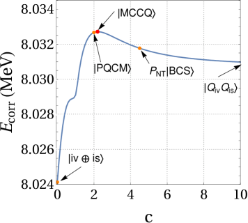
Figure 1: Correlation energy vs the $c$ coefficient of the $n_{q}=2$ collective quartet ansatz of Eq. (14), for the nucleus ¹⁰⁸Xe. The orange dots indicated by arrows refer to the states $|\text{iv}\oplus\text{is}\rangle$ of Eq. (10) with $c=0$, $|PQCM\rangle$ of Eq. (2) with $c=2$, $\mathcal{P}_{NT}|BCS\rangle$ of Eq. (6) with $c=4.47$. The state $|Q_{\text{iv}}Q_{\text{is}}\rangle=Q_{\text{iv}}^{\dagger}(x)Q_{\text{is}}^{\dagger}(y)|0\rangle$ corresponds to the limit $c\rightarrow\infty$. The Maximally Correlated Collective Quartet state $|MCCQ\rangle$ with $c=2.2$ (the red dot on the graph) displays the largest correlation energy.

4 Summary and Conclusions

In this work we analyzed the structure of the quartetting ground state of the isovector-isoscalar pairing Hamiltonian for axially-deformed $N=Z$ nuclei. The most general collective quartet state involves all terms built from various numbers of isovector and isoscalar quartet structures. Notable particular examples include the PQCM condensate ansatz and the particle number and isospin projected BCS state. While the functional dependency on the variational amplitudes may differ, the numerical agreement between all collective quartet states is excellent. This is due to the high overlap between the isovector and isoscalar quartet structures, which generally leads to a strong mixing of the two types of correlations in the quartetting approach. This contrasts with the expectation from the mean field picture, where the isovector and isoscalar correlations do not coexist in $N=Z$ nuclei. As opposed to the spherical mean field approach of Ref. gez11 , the present quartetting approach for deformed nuclei indicates dominating isovector correlations in the region above $N=Z=60$. Full symmetry restoration of the quartetting wavefunction (i.e. including angular momentum projection) is currently under consideration for an improved description of the isovector-isoscalar interplay in realistic scenarios.

- (1) A. Bohr, B.R. Mottelson, D. Pines, Phys. Rev. 110, 936 (1958)
- (2) S. Frauendorf, A. Macchiavelli, Progress in Particle and Nuclear Physics 78, 24 (2014)
- (3) J.A. Sheikh, J. Dobaczewski, P. Ring, L.M. Robledo, C. Yannouleas (2019), 1901.06992
- (4) N. Sandulescu, D. Negrea, C.W. Johnson, Phys. Rev. C 86, 041302(R) (2012)
- (5) N. Sandulescu, D. Negrea, J. Dukelsky, C.W. Johnson, Phys. Rev. C 85, 061303(R) (2012)
- (6) N. Sandulescu, D. Negrea, J. Dukelsky, C.W. Johnson, Journal of Physics: Conference Series 533, 012018 (2014)
- (7) N. Sandulescu, D. Negrea, D. Gambacurta, Physics Letters B 751, 348 (2015)
- (8) M. Sambataro, N. Sandulescu, Phys. Rev. Lett. 115, 112501 (2015)
- (9) M. Sambataro, N. Sandulescu, Phys. Rev. C 91, 064318 (2015)
- (10) M. Sambataro, N. Sandulescu, Physics Letters B 763, 151 (2016)
- (11) M. Sambataro, N. Sandulescu, The European Physical Journal A 53, 47 (2017)
- (12) D. Negrea, P. Buganu, D. Gambacurta, N. Sandulescu, Phys. Rev. C 98, 064319 (2018)
- (13) J. Dobes, S. Pittel, Phys. Rev. C 57, 688 (1998)
- (14) N. Sandulescu, B. Errea, J. Dukelsky, Phys. Rev. C 80, 044335 (2009)
- (15) A. Romero, J. Dobaczewski, A. Pastore, Physics Letters B 795, 177 (2019)
- (16) V.V. Baran, D.R. Nichita, D. Negrea, D.S. Delion, N. Sandulescu, P. Schuck (2020), arXiv: 2009.00932
- (17) M. Sambataro, N. Sandulescu, C. Johnson, Physics Letters B 740, 137 (2015)
- (18) T. Sogo, R. Lazauskas, G. Röpke, P. Schuck, Phys. Rev. C 79, 051301(R) (2009)
- (19) A. Tohsaki, H. Horiuchi, P. Schuck, G. Röpke, Phys. Rev. Lett. 87, 192501 (2001)
- (20) V.V. Baran, D.S. Delion, Phys. Lett. B 805, 135462 (2020)
- (21) M. Fellah, T.F. Hammann, D.E. Medjadi, Phys. Rev. C 8, 1585 (1973)
- (22) P. Bonche, H. Flocard, P. Heenen, Computer Physics Communications 171, 49 (2005)
- (23) E. Chabanat, P. Bonche, P. Haensel, J. Meyer, R. Schaeffer, Nuclear Physics A 627, 710 (1997)
- (24) G.F. Bertsch, Y. Luo, Phys. Rev. C 81, 064320 (2010)
- (25) A. Gezerlis, G.F. Bertsch, Y.L. Luo, Phys. Rev. Lett. 106, 252502 (2011)