The solar gravitational redshift from HARPS-LFC
Moon spectra ^,

Abstract

Context. The general theory of relativity predicts the redshift of spectral lines in the solar photosphere as a consequence of the gravitational potential of the Sun. This effect can be measured from a solar disk-integrated flux spectrum of the Sun’s reflected light on Solar System bodies.

Aims. The laser frequency comb (LFC) calibration system attached to the HARPS spectrograph offers the possibility of performing an accurate measurement of the solar gravitational redshift (GRS) by observing the Moon or other Solar System bodies. Here, we analyse the line shift observed in Fe absorption lines from five high-quality HARPS-LFC spectra of the Moon.

Methods. We selected an initial sample of 326 photospheric Fe lines in the spectral range between 476–585 nm and measured their line positions and equivalent widths (EWs). Accurate line shifts were derived from the wavelength position of the core of the lines compared with the laboratory wavelengths of Fe lines. We also used a CO⁵BOLD 3D hydrodynamical model atmosphere of the Sun to compute 3D synthetic line profiles of a subsample of about 200 spectral Fe lines centred at their laboratory wavelengths. We fit the observed relatively weak spectral Fe lines (with EW$<180$ ${\rm m{\AA}}$) with the 3D synthetic profiles.

Results. Convective motions in the solar photosphere do not affect the line cores of Fe lines stronger than about $\sim 150$ ${\rm m{\AA}}$. In our sample, only 15 Fe i lines have EWs in the range $150<$ EW(${\rm m{\AA}}$) $<550$, providing a measurement of the solar GRS at $639\pm 14$ ${\rm m\;s^{-1}}$, which is consistent with the expected theoretical value on Earth of $\sim 633.1$ ${\rm m\;s^{-1}}$. A final sample of about 97 weak Fe lines with EW $<180$ ${\rm m{\AA}}$ allows us to derive a mean global line shift of $638\pm 6$ ${\rm m\;s^{-1}}$, which is in agreement with the theoretical solar GRS.

Conclusions. These are the most accurate measurements of the solar GRS obtained thus far. Ultrastable spectrographs calibrated with the LFC over a larger spectral range, such as HARPS or ESPRESSO, together with a further improvement on the laboratory wavelengths, could provide a more robust measurement of the solar GRS and further testing of 3D hydrodynamical models.

1 Introduction

The general theory of relativity (Einstein, 1911, 1916) predicts the gravitational redshift of spectral lines in the solar photosphere. However, the effects of gravity on light were first demonstrated by light deflection during a solar eclipse and by its magnified effects in white dwarfs (Greenstein & Trimble, 1972). In the Sun, the gravitational redshift is competing with the blueshift of the lines due to the convective motions. Convection produces granulation phenomena, which induce line shifts which are opposite to the gravitational redshift. The granulation pattern is formed by upward flows with a velocity of 1-2 ${\rm km\;s^{-1}}$in the inner parts of the granules and downward flows in the intergranular lanes, which are faster by a factor of between two and three (Dravins et al., 1981; Dravins, 1990). The granulation pattern has a scale size of 0.6-1.3 Mm and a lifetime of about 8-12 min (Spruit et al., 1990; Hirzberger et al., 1999; Schrijver, 2000). Larger scale sizes of 15-30 and 5-10 Mm and lifetimes of 20-30 hr and $\sim 2$ hr are also present, and referred to as supergranulation and mesogranulation, which produce vertical raising velocities of 40-60 ${\rm m\;s^{-1}}$, respectively (Schrijver, 2000), with larger horizontal velocities and more relevant, perhaps, towards the solar limb.

This complex granulation pattern produces asymmetric disk-integrated photospheric lines with observed Doppler blue shifts down to $\sim-500$ ${\rm m\;s^{-1}}$ (Allende Prieto & Garcia Lopez, 1998b; Reiners et al., 2016) after subtracting the theoretical value of the solar gravitational redshift. Granulation is also variable and on timescales larger than 1 hr could produce radial velocity (RV) variations of $\sim 1$ ${\rm m\;s^{-1}}$ (Meunier et al., 2015). In addition, the $\sim 5$ min solar oscillations are associated with a vertical velocity component of $\sim 0.4$ ${\rm km\;s^{-1}}$ (Keil & Canfield, 1978), producing a RV signature in disk-integrated light of only 0.1-4 ${\rm m\;s^{-1}}$ (Dumusque et al., 2011).

Active regions, mainly spots and faculae, with a lifetime of 10-50 days, located at different positions of the solar disk as the Sun rotates, can also yield RV signatures of about 0.4 ${\rm m\;s^{-1}}$ due to the flux imbalance and about 2.4 ${\rm m\;s^{-1}}$ from the suppression of convective motions in magnetic regions (Lagrange et al., 2010; Meunier et al., 2010a; Haywood et al., 2016). The inhibition of convection appears to be the dominant source of RV variations during the solar cycle, with an amplitude of 8-10 ${\rm m\;s^{-1}}$ (Meunier et al., 2010a, b; Lanza et al., 2016).

The modelling of granulation has been done using empirical models that are relatively simple, consisting of between two and four components (Dravins et al., 1981; Dravins, 1990) or complex hydrodynamical simulations, including magnetic fields (e.g. Cegla et al., 2013). Hydrodynamical simulations have also been able to fairly reproduce the shapes and absolute shifts of Fe i lines (Asplund et al., 2000). The convective blueshift caused by the granulation pattern can be explained as flux-dominant rising granules whose velocity diminishes with height. Strong and weak lines form generally in the outer and inner layers, respectively, of the photosphere (Magain, 1986; Grossmann-Doerth, 1994; Gray, 2005). Thus, cores of stronger lines forming in outer layers of the photosphere show smaller convective blueshifts than weaker lines forming deeper in the photosphere. Therefore, the Doppler shifts of strong lines may, in principle, mostly be associated to the gravitational redshift.

The accuracy of line positions in the solar spectra has been extensively investigated and some solar line atlases have been published in recent decades (e.g. Allende Prieto & Garcia Lopez, 1998a; Molaro & Monai, 2012), using Fourier transform spectrometer (FTS) observations of the Sun (Kurucz et al., 1984; Wallace et al., 2011). The wavelength positions of solar lines in the Kitt Peak FTS spectra (Kurucz et al., 1984) have an uncertainty of 50-150 ${\rm m\;s^{-1}}$ and zero offset of about 100 ${\rm m\;s^{-1}}$ (Allende Prieto & Garcia Lopez, 1998a; Molaro & Centurión, 2011). The line precision and accuracy has been improved to 45-90 ${\rm m\;s^{-1}}$ with HARPS observations of solar spectra obtained from asteroids (Molaro & Centurión, 2011; Molaro & Monai, 2012; Lanza & Molaro, 2015). Using HARPS spectra of the Moon wavelength calibrated with the laser frequency comb, Molaro et al. (2013) produced a solar atlas in the region 480-580 nm with a mean accuracy of $\sim 12$ ${\rm m\;s^{-1}}$. Reiners et al. (2016) obtained a new solar atlas from observations of disk-integrated FTS spectra. The radial velocity is consistent with that of the HARPS-LFC at the level of few ${\rm m\;s^{-1}}$, thus confirming the systematic offset of 100 ${\rm m\;s^{-1}}$ of the Keat Peak solar spectrum of Kurucz et al. (1984); Wallace et al. (2011).

The general theory of relativity (Einstein, 1911, 1916) predicts the gravitational redshift of spectral lines in the solar photosphere as $v_{\rm GRS,\odot}=(GM_{\odot}/cR_{\odot})$, where $G$ is the gravitational constant, $c$ is the speed of light, and $M_{\odot}$ and $R_{\odot}$ are the mass and radius of the Sun, respectively. Using the nominal values of the astronomical constants recommended by the IAU (Prša et al., 2016), this equation gives $v_{\rm GRS,\odot}=636.31$ ${\rm m\;s^{-1}}$. The same effect from the solar photosphere to 1 AU (Allende Prieto et al., 2009; Roca Cortés & Pallé, 2014) amounts to:

$$v_{\rm GRS,1{\rm AU}}=\frac{GM_{\odot}}{c}\left(\frac{1}{R_{\odot}}-\frac{1}{\rm 1AU}\right)=633.35{\rm\;m\;s}^{-1}.$$

The distance of the Earth on 25 November 2010 was of 147.75 millions km, which leads to a small correction of about +4 ${\rm cm\;s^{-1}}$. The gravitational effect of the Moon is zero since it is a reflection, however, in accounting for the gravitational potential of the Earth, $v_{\rm GRS,\oplus}=(GM_{\oplus}/cR_{\oplus})=0.21$ ${\rm m\;s^{-1}}$, where $M_{\oplus}$ and $R_{\oplus}$  are the nominal mass and radius of the Earth, we get a final value of:

$$v_{\rm GRS,{\rm theo}}=v_{\rm GRS,1{\rm AU}}-v_{\rm GRS,\oplus}=633.10{\rm\;m\;s}^{-1}.$$

The solar GRS effect is quite large and it may seem rather surprising that it has never been measured with high accuracy. We can roughly divide the attempts in two categories: observations of single lines in resolved regions of the solar disk and observations of the integrated solar disk, usually done with stellar spectrographs. The first class of observations usually demonstrate quite a high level of precision, but they are limited by the fact that, with the exception of sunspot umbrae, each fraction of the solar surface is subject to peculiar velocities (Beckers, 1977).

Using the solar disk-integrated atlases, various authors have provided an observational measurement of the solar GRS from strong lines in the solar photosphere, with values close to the theoretical prediction: $v_{\rm GRS,{\rm obs}}=612\pm 58$ ${\rm m\;s^{-1}}$ (Allende Prieto & Garcia Lopez, 1998b), $v_{\rm GRS,{\rm obs}}=601\pm 43$ ${\rm m\;s^{-1}}$ (Molaro & Monai, 2012). Using solar spectra in the small spectral region 5188–5212 Å calibrated with an iodine-cell, Takeda & Ueno (2012) obtained a result of $v_{\rm GRS,{\rm obs}}=698\pm 133$ ${\rm m\;s^{-1}}$. More recently, Roca Cortés & Pallé (2014) presented disk-integrated sunlight observations centred on the K I 7699 Å line with a spectral width of 15 Å over an extended period, between 1976–2013, to derive $v_{\rm GRS,{\rm obs}}=600.4\pm 0.8$ ${\rm m\;s^{-1}}$, with an amplitude of $\pm 5$ ${\rm m\;s^{-1}}$, which is which is in anti-correlation with regard to the solar magnetic cycle.

Resolved observations suffer from the peculiar motions on the solar surface, whereas integrated disk observations suffer from the limited accuracy of traditional spectrographs. With the advent of a new generation of exoplanet hunters, such as HARPS, and the use of calibration systems based on laser frequency combs, solar observations are now capable of reaching the required level of accuracy.

The laser frequency comb (LFC) is a new wavelength calibration system for high-resolution astronomical spectrographs which has been tested on the HARPS spectrograph (Wilken et al., 2010, 2012). In terms of the determination of individual line positions, Th-Ar lamps can achieve an accuracy on the level of several tens of ${\rm m\;s^{-1}}$ (Lo Curto et al., 2012; Palmer & Engleman, 1983). When accounting for the several thousand lines available in the spectral range of HARPS, the overall precision can be increased by about a factor of 100, with limitations related to the blending of lines, non-uniform density of Th lines across the spectrum, and lamp aging. We should note that for determining the solar GRS, we need to measure the absolute wavelength of spectral lines and, therefore, wavelength accuracy (rather than precision) is the most relevant parameter. The comparison of line positions of LFC and Th-Ar calibrated spectra in the HARPS spectrograph have revealed S-type distortions on each order along the whole spectral range with an amplitude of $\pm 40$ ${\rm m\;s^{-1}}$ and whose precise shape is also wavelength-dependent (Molaro et al., 2013). Several test campaigns of the LFC coupled to HARPS have demonstrated that its calibration can give a short-term repeatability of 2.5 ${\rm cm\;s^{-1}}$ (Wilken et al., 2012), while Th-Ar lamps can only reach a photon noise level of 10 ${\rm cm\;s^{-1}}$. In addition, the RV precision of Th-Ar lamps is about 30 ${\rm cm\;s^{-1}}$ (e.g. Lo Curto et al., 2010). Very recently, Probst et al. (2020) demonstrated repeatability of the line positions of the upgraded HARPS LFC system down to the photon noise level of 1 ${\rm cm\;s^{-1}}$, as compared with the 10 ${\rm cm\;s^{-1}}$ level reached by Th-Ar lamps, opening up a new horizon for current and future ultra-stable high-resolution spectrographs, along with bringing new science frontiers closer, such as the detection of Earth twins orbiting Sun-like stars in their habitable zone. The same authors have also shown that wavelength calibrations obtained with two separate LFCs on HARPS were consistent to better than 60 ${\rm cm\;s^{-1}}$ (see also Milaković et al., 2020). In this work, we exploit the high accuracy of the LFC wavelength solution using LFC calibrated HARPS spectra of the Sun’s light reflected on the Moon (Molaro et al., 2013) to measure the solar gravitational redshift as a test of the general theory of relativity (Einstein, 1916).

2 Observations and data analysis

We performed observations of the Moon on 25 November 2010 with the HARPS spectrograph installed at the 3.6m-ESO telescope in the Observatorio de La Silla (see Table 1). HARPS is a cross-dispersed echelle, high-resolution spectrograph fed with two fibres of 1-arcsec aperture on sky (fiber A: science and fiber B: calibration), which follow approximately the same optical path (Mayor et al., 2003). The HARPS fibers are equipped with a double scrambler to provide both image and pupil stability, which is an important difference with respect to spectrographs fed through a slit, where a non-uniform slit illumination induces radial velocity differences between different exposures. HARPS is an ultra-stable instrument with the capacity to achieve both short-term and long-term precision below 0.8 ${\rm m\;s^{-1}}$ (Pepe et al., 2011, 2014). The calibration on fiber B is used to track the instrument drift, typically below $\pm 1$ ${\rm m\;s^{-1}}$, during night observations with respect to afternoon calibrations (Mayor et al., 2003).

Table 1: Log of observations

UT(start)	Label	$T_{\rm exp}$	RVc	S/N
h:m:s		s	${\rm km\;s^{-1}}$
05:47:20.802	s802	60	$-1.190$	241-286-330
05:49:42.429	s429	150	$-1.187$	383-457-524
05:53:19.301	s301	60	$-1.182$	245-293-337
05:55:20.898	s898	120	$-1.179$	371-443-509
05:57:54.476	s476	120	$-1.176$	383-457-526
NOTE. - UT at start, exposure times, $T_{\rm exp}$, expected radial
velocity computed with JPL ephemerides, RVc, signal to
noise at centre of order 34, 45 and 57 of the HARPS-LFC
observations of the Moon carried out on 25 November 2010.

HARPS provides a median resolving power of $R=\lambda/\delta\lambda\sim 115,000$ covering the spectral range of 380–690 nm distributed over 72 spectral echelle orders, with a small gap at 530-539 nm. The LFC consists of thousands of lines that are equally spaced in frequency and can be described with a simple equation $f=f_{\rm off}+nf_{\rm rep}$, where $f_{\rm rep}$ is the repetition frequency (that is, the frequency difference between adjacent lines) and $f_{\rm off}$ is the offset frequency, and $n$ is an integer that is commonly referred to as the mode number. The LFC is linked to an atomic clock which ensures an extremely high accuracy (better than 1 m/s) and long-term stability (Wilken et al., 2012; Lo Curto et al., 2012). The LFC, as described in Wilken et al. (2012), uses three concatenated Fabry-Perot cavities to filter the unwanted modes to a line spacing of $f_{\rm rep}=18$ GHz. This is followed by a frequency doubling of the LFC spectrum to centre it at about 525 nm and subsequent spectral broadening in a tapered photonic crystal fibre. Thus, the LFC is imaged onto both HARPS blue and red chips covering a wavelength range of about 125 nm, spanning from 465 to 590 nm, from spectral order #34 to #57 of the 72 orders of HARPS.

The LFC offers about 350 lines (usually called modes) per spectral order equally spaced in frequency and with similar intensity (as a comparison, Th-Ar lamps offer less than 100 lines per spectral order with very different intensities, sometimes blended or even saturated). This allows for wavelength calibrations of a fraction of an order and we separately calibrated each of the eight master lithographic blocks of 512 pixels in the dispersion direction (Molaro et al., 2013). HARPS blue and red chips are, in fact, built up with 16 master blocks of 1024 x 512 pixels. The use of the LFC allowed us to discover the S-type distortions and up to about 70 ${\rm m\;s^{-1}}$ ‘jumps’ in the wavelength solutions between adjacent master blocks associated to different pixel sizes along the stitching borders of these blocks (Wilken et al., 2010; Milaković et al., 2020).

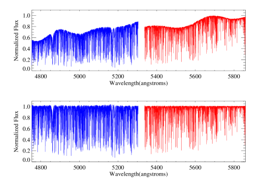
Figure 1: Top panel: Blaze-corrected, co-added, merged HARPS-LFC spectrum of the Moon for both blue and red chips of HARPS. Bottom panel: Normalised (order-by-order), merged HARPS-LFC spectrum.

HARPS-LFC spectra of the Sun’s reflected light on the Moon were collected pointing to the Moon’s centre. During these observations, 86% of the Moon was illuminated. Five HARPS spectra of the Moon on fiber A were taken with simultaneous LFC calibration on fiber B, providing a simultaneous reference spectrum to monitor overnight instrumental drifts. The instrumental drift is computed from the displacement in pixels of the LFC spectrum acquired on fiber B (simultaneously with the Moon spectra on fiber A) with respect to a reference LFC spectrum. For each LFC mode the displacement is weighted by the signal collected on that mode. The HARPS-LFC observations cover a time span of 10 min, ensuring that solar oscillations should be averaged out. The exposure times varies between 60 to 150 seconds, providing signal-to-noise ratios (S/N) in the range between $\sim 290-460$ (see Table 1). Each spectrum was reduced using the standard HARPS pipeline and the LFC frames were calibrated using eight third-degree polynomials corresponding to the eight master blocks of 512 pixels. These LFC wavelength calibrated 2D order spectra were blaze-corrected using the blaze function of each order. We then normalised these 2D spectra order by order with a third-order polynomial using our own automated IDL-based routine. The normalised spectra after order merging were rebinned to a constant wavelength step of 0.01 Å pixel^-1 equivalent to $\sim 0.8$ ${\rm km\;s^{-1}}$ pixel^-1. Each spectrum was corrected for radial velocity (see Table 1) using the JPL ephemeris to place them in the laboratory rest frame (see Molaro et al., 2013, for further details). The computed radial velocity accounts for the motions of the Moon with respect to the observer and the Sun, and also includes a component of 3.2 ${\rm m\;s^{-1}}$ due to the rotation of the Moon, since the sunlight impacts the receding lunar hemisphere before being reflected at an angle of $43^{\circ}$ at the time of the observation. In Fig. 1 we display the merged, normalised spectrum one of the five Moon HARPS-LFC spectra. A proper normalisation procedure is very relevant for the determination of the line core centres of individual Fe lines.

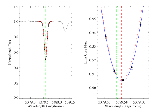
Figure 2: Example of the line core fit of the line Fe i $\lambda_{\rm lab}$ 5379.5740 Å described in Section 3. Left panel: Normalised flux of a HARPS-LFC spectrum (black thin line) of the Moon, labelled s429 in Table 1, centred on $\lambda_{\rm lab}=5379.5740$ Å together with a single Gaussian fit (red dashed line) in a region of 0.5 Å (vertical red dashed lines) centred on the laboratory wavelength (vertical green dashed-dotted line). Right panel: Parabolic fit (blue solid line) to five points of the line core compared to the single Gaussian fit (red dashed line). Vertical lines show the wavelength position of the centroids of the parabolic fit (blue dashed-three dotted line) and the Gaussian fit (red dashed line), together with the laboratory wavelength (vertical green dashed-dotted line).

3 Line core shifts

We selected Fe lines from the linelists in previous works (Sousa et al., 2007; Molaro et al., 2013) available in the spectral range 465–590 nm, complemented with Fe lines extracted from the Vienna Atomic Line Database (VALD Piskunov et al., 1995), using the extract stellar option with solar parameters. We search for apparently isolated Fe i and Fe ii lines by visually inspecting the HARPS-LFC spectrum of the Moon with the IRAF package splot. The atomic line parameters of Fe lines were adopted from VALD, including wavelength, excitation potential, and oscillator strength. We also collect, for these Fe lines, the laboratory wavelengths from Nave et al. (1994); Nave (2012); Nave & Johansson (2013). We note that the laboratory wavelengths of Fe i lines with a quality flag labelled with A have an accuracy in the range $0.28-1.25$ ${\rm m{\AA}}$, corresponding to $16-75$ ${\rm m\;s^{-1}}$ (Nave et al., 1994). Those lines flagged as B, C, D have uncertainties in the range $0.4-2.5$ ${\rm m{\AA}}$, $0.8-5.0$ ${\rm m{\AA}}$, and $>5.0$ ${\rm m{\AA}}$, corresponding to $24-150$ ${\rm m\;s^{-1}}$, $48-300$ ${\rm m\;s^{-1}}$,$>300$ ${\rm m\;s^{-1}}$ (Nave et al., 1994). The final linelist contains 326 Fe lines, 200 in the blue CCD and 126 in the red CCD. Among these lines there are 152, 42, 3, 3 lines in the blue chip and 101, 15, 3, 7 lines in the red chip with flags A, B, C, D, respectively. There are only four Fe ii lines in the blue chip that have uncertainties in the range of $0.2-0.9$ ${\rm m{\AA}}$, i.e. $12-51$ ${\rm m\;s^{-1}}$ (Nave & Johansson, 2013).

Nave & Sansonetti (2011) discussed the calibration of wavenumber measurements used to infer the original published wavelengths of Fe lines (Nave et al., 1994). They used 28 Ar ii lines as wavenumber standards based on the results in Norlén (1973), that were subsequently remeasured by Whaling et al. (1995), providing, in principle, a higher precision and accuracy. They suggested to increase the wavenumber measurements of Fe i by $6.7\pm 0.8$ parts in $10^{8}$. We have downloaded, from the NIST Atomic Spectra Database, the wavelengths of Fe lines, together with the Ritz wavelengths derived from the recalibrated energy levels, both with the same constant quantity of $6.7$ parts in $10^{8}$ (Kramida et al., 2019). These wavelengths are shorter, on average, by about 20 and 35 ${\rm m\;s^{-1}}$, respectively, compared to the original wavelengths in Nave et al. (1994). The mean uncertainties on wavelengths also extracted from NIST database are 1.1 and 0.4 ${\rm m{\AA}}$ corresponding to 64 and 23 ${\rm m\;s^{-1}}$. Throughout this work, we use as our laboratory wavelengths, $\lambda_{\rm lab}$, the original wavelengths in Nave et al. (1994) and we discuss in Section 6 how the results change when using the recalibrated wavelengths, $\lambda_{\rm nist}$, and the recalibrated Ritz wavelengths, $\lambda_{\rm ritz}$, as given in Table A.1.

The equivalent widths (EWs) of the 326 lines were measured with the TAME (Kang & Lee, 2012) code, which uses a linelist extracted from VALD to identify nearby spectral lines that can affect the EW determination of a given spectral line and performs a multi-Gaussian fit to a spectral range of a few angstroms. For a few strong lines with EWs greater than 170 ${\rm m{\AA}}$ blended with weaker lines, we use the splot tool within IRAF package to fit them using a Lorentzian function to account for the strong wings of those spectral lines. There were also several weaker lines with some peculiarities for which TAME fails to provide a good fit, so we additionally measured their EWs with the splot tool. A total of six and nine Fe lines in the blue and red chip were measured with IRAF.

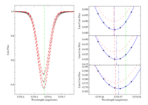
Figure 3: Example of line core fit of the 3D profiles of the line Fe i $\lambda_{\rm lab}$ 5379.5740 Å described in Section 4. Left panel: Line 3D profiles for three line strengths at solar abundance $\pm 0.1$ dex (black dots) together with single Gaussian fits (red dashed lines) and the laboratory wavelength (vertical green dashed-dotted line). Right panels: Parabolic fits (blue solid line) to the line core of the three 3D profiles, together with single Gaussian fits (red dashed lines). Vertical lines show the wavelength position of the centroids of the parabolic fit (blue dashed-three dotted line) and the Gaussian fit (red dashed line), together with the laboratory wavelength (vertical green dashed-dotted line).

The TAME output provides both a linelist with laboratory wavelengths and expected depths in the solar photosphere extracted from VALD and a linelist with the identified lines and fitted wavelengths and EWs. This allows us to identify possible line blends of Fe i, Fe ii, or other element species with wavelengths closer than 0.15 Å and depths greater and 0.5 times the depth of the fitted Fe line. With this rule, we classified 38 and 16 lines as blended Fe lines in the blue and red chips. We visually inspected the output of the TAME code to see if the multi-Gaussian fits were reasonable. In a few cases, we detected some Fe lines with blends that are not present in the linelists extracted from VALD and we classified these lines as problematic. TAME also performs an automatic local continuum fit to the highest flux point and, in some cases, due to surrounding weak lines or close-by very strong lines, this procedure fails. We identified these lines and labelled them as problematic. These 11 and 4 Fe lines in the blue and red chips, respectively, were also discarded. Thus, a total of 69 Fe lines were discarded from the initial list of 326. Only two Fe ii lines in the blue chip fulfilled these criteria.

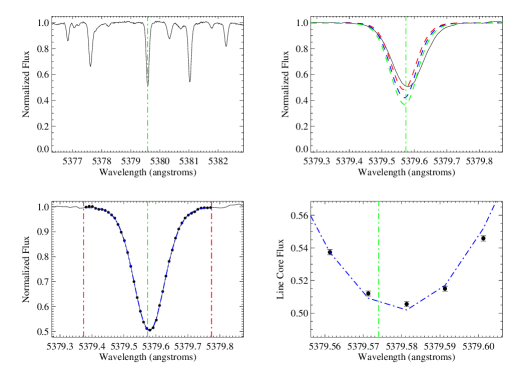
Figure 4: Example of global line fit of the line Fe i $\lambda_{\rm lab}$ 5379.5740 Å described in Section 5. Top-left panel: Normalised flux of a HARPS-LFC spectrum (black thin line) of the Moon, labelled s429 in Table 1, centred on $\lambda_{\rm lab}=5379.5740$ Å as a vertical green dashed-dotted line. Top-right panel: Observed line profile together with unbroadened 3D line profiles of three different strengths. Bottom-left panel: Global line fit (blue dashed-dotted line) to the line flux points within the spectral region of 0.4 Å (region within the vertical red dashed-dotted lines) centred on the laboratory wavelength (vertical green dashed-dotted line). Bottom-right panel: Line core flux points (black dots) and global line fit (blue dashed-dotted line) with the laboratory wavelength (vertical green dashed-dotted line) shown as reference.

We fitted the line cores of the remaining 257 Fe lines using our own automated IDL-based routine, shown in Fig. 2. We identified the line cores with the laboratory wavelengths (Nave et al., 1994; Nave, 2012; Nave & Johansson, 2013) of the spectral lines in a spectral range of $\sim$0.5 Å. We fitted a single Gaussian to the line and selected the five flux points of the line core from the Gaussian centre and the minimum flux point of the line. We derived the centre of the line core from a parabolic fit to these five flux points. In Fig. 2, we display an example of the line core fit to the observed Fe i $\lambda_{\rm lab}$ 5379.5740 Å line, with an EW of $60.2\pm 1.2$ mÅ, using a parabolic fit that clearly provides a better centroid of the line core than a single Gaussian fit. The line core shift is computed as $v_{\rm core,obs}=c(\lambda_{\rm core,obs}-\lambda_{\rm lab})/\lambda_{\rm lab}$, where $\lambda_{\rm lab}$ is the laboratory wavelength and $\lambda_{\rm core,obs}$ is the wavelength centroid of the parabolic fit. The centroid of the line core is clearly redshifted with respect to the laboratory wavelength $\lambda_{\rm lab}=5379.5740$ Å by $v_{\rm core,obs}=346.6\pm 18.4$ ${\rm m\;s^{-1}}$. We carried out the same exercise for each Fe line of each of the five HARPS-LFC spectra of the Moon. The value and uncertainty of the EW and of the line core shift are the mean and standard deviation, respectively, as resulting from the five measurements of the five HARPS-LFC spectra.

4 3D line profiles

Synthetic 3D line profiles are based on a time-dependent, 3D, hydro-dynamical model atmosphere of the Sun computed with the CO⁵BOLD (Freytag et al., 2002) code. The 3D model atmosphere has a box size of $5.6\times 5.6\times 2.27$ Mm³, a resolution of $140\times 140\times 150$ ($N_{X}\times N_{Y}\times N_{Z}$) grid points (Caffau et al., 2011), and spans a range, in Rosseland optical depth, of about $-6.7<\log\tau_{\rm Ross}<5.5$ (from -1.4 Mm below to +0.9 Mm above $\tau_{\rm Ross}=1$). We selected 20 representative snapshots from the full time sequence to reduce the computing burden of the spectral synthesis calculations. These snapshots are equidistantly spaced in time, sufficiently separated in time to show little correlation, and cover 1.2 hours of solar time. The 3D model atmosphere has a temporal average effective temperature of $\left<T_{\rm eff}\right>=5780$ K, a surface gravity of $\log g=4.4$, and a metallicity of [Fe/H]$=0$ with A(Fe)=7.52. The solar reference abundances are those given in Caffau et al. (2011). The non-local radiative transfer is solved in 12 opacity bins on the standard grid of $140\times 140\times 150$ cells (see Ludwig et al., 2009, for further details on 3D hydrodynamical model atmospheres). The radiative heating terms are computed by solving the non-local LTE transfer equation on a ray system of long characteristics for 12 opacity bins. The synthetic line profiles are computed with the line formation code Linfor3D, taking into account the detailed 3D thermal structure and hydrodynamical velocity field of the selected snapshots. The adopted resolving power was 1666666, giving a velocity sampling of about 0.2 ${\rm km\;s^{-1}}$. We use a vertical and three inclined angles and four azimuth angles (Freytag et al., 2012). We use the default broadening theory adopted in Linfor3D, which uses the standard Unsöld theory that assumes a van der Waals interaction between the absorbing atom and the perturbing hydrogen atom, which, in principle, could have an impact on the wings of strong lines but not on the core of the lines. The statistical uncertainty on the wavelength position of the temporally and horizontally averaged 3D profiles is about 30 ${\rm m\;s^{-1}}$, estimated from the dispersion of individual snapshots and from the comparison with other solar models.

In Fig. 3, we display an example of the 3D line profiles of the Fe i 5379.5740 Å line for three different line strengths computed by changing the oscillator strengths, $\log gf$, in the 3D spectral synthesis by -0.1, 0.0 and +0.1 dex, respectively. We ran 3D spectral synthesis for a subsample of 205 Fe lines, with 112 and 93 lines in the blue and in the red chips, respectively. The wavelength centroid of the core of these lines were measured using a similar approach as for the observed line cores. Figure 3 shows the position of the line cores of three different 3D profiles for the three $gf$ values with EWs of 53.2, 62.1 and 71.0 ${\rm m{\AA}}$, providing a theoretical core shift of $-345.3$, $-280.9$ and $-215.2$ ${\rm m\;s^{-1}}$, respectively, for these three 3D profiles with respect to the laboratory wavelength of the Fe i 5379.5740 Å line. The theoretical core shift (always negative since there is no solar GRS added in the 3D model) gets closer to zero as the line gets stronger, so the convective blue shifts is smaller as the lines gets stronger. We performed a linear interpolation with the observed EW to infer a line core shift of $-294.6$ ${\rm m\;s^{-1}}$ for the Fe i 5379.5740 Å line, with an EW of $60.2\pm 1.2$ mÅ. The 3D model provides a qualitative and quantitative description of the granulation phenomena, where the weaker the lines are the more blue shifted, as expected. Subtracting the line core shift derived from the 3D line profile, $v_{\rm core,3D}=-294.6$ ${\rm m\;s^{-1}}$ to the observed line core shift of the observed line Fe i $\lambda_{\rm lab}$ 5379.5740 Å, $v_{\rm core,obs}=346.6\pm 18.4$ ${\rm m\;s^{-1}}$, should provide a value of the solar gravitational redshift, $v_{\rm GRS,obs}=641.2\pm 18.4$ ${\rm m\;s^{-1}}$, which is in agreement with the theoretical value of 633.10 ${\rm m\;s^{-1}}$.

5 3D global line shifts

We also performed the global fit of the observed line profiles using the 3D synthetic profiles. For each observed line, a grid of 3D synthetic profiles is created for three different values of Fe abundance (A(Fe)$=7.42$, 7.52 and 7.62) and rotational broadening ($v_{\rm ROT}=0$, 2, and 4 ${\rm km\;s^{-1}}$). The grid is first broadened using the code LinforRotate (Ludwig, 2007) and later with a Gaussian instrumental profile with a full width half maximum (FWHM) equivalent to the resolving power $R=115,000$ ($v_{\rm INS}=2.61$ ${\rm km\;s^{-1}}$). We performed a global fit of every Fe line using our automated IDL-based routine that makes use of the MPFIT routine (Markwardt, 2009), including three free parameters: rotational broadening, velocity shift, and iron abundance. The continuum location was fixed at 1. We ran this routine to fit the subsample of Fe lines for the five HARPS-LFC spectra.

In Fig. 4, we show an example of the global line fit to the Fe i $\lambda_{\rm lab}$ 5379.5740 Å line. The fit is done in a wavelength range of 0.5 Å centred on the laboratory wavelength. The 3D synthetic profile matches quite well the observed line profile, although, as shown in the bottom-right panel of Fig. 4, the 3D synthetic profile does not perfectly fit the line core. From the fit of this spectral line in the spectrum s429 (see Table 1), we infer a global velocity shift of $v_{\rm fit,3D}=648.4\pm 4.8$ ${\rm m\;s^{-1}}$ with a solar abundance of A(Fe)$=7.526\pm 0.001$ dex and $v_{\rm ROT}=1.72\pm 0.06$ ${\rm km\;s^{-1}}$. Both the iron abundance and the rotational velocity are consistent with their expected solar values. The expected rotational velocity of the Sun is $v\sin i=1.8\pm 0.2$ ${\rm km\;s^{-1}}$ (see e.g. Gray, 2018). The mean rotation and Fe abundance values found for the final set of fitted Fe lines are 2.5 ${\rm km\;s^{-1}}$ and 7.59 dex with a standard deviation of 0.5 ${\rm km\;s^{-1}}$ and 0.09 dex. The derived velocity shift is close although not consistent with regard to the theoretical value of the solar gravitational redshift, $v_{\rm GRS,theo}=633.1$ ${\rm m\;s^{-1}}$. The result depends on the accuracy of the laboratory wavelength, with an uncertainty of $>16$ ${\rm m\;s^{-1}}$ for lines labelled as A, as well as the precision of the 3D profile, with an uncertainty of about 30 ${\rm m\;s^{-1}}$. Hence, a deviation $\sim 15$ ${\rm m\;s^{-1}}$ is within this error.

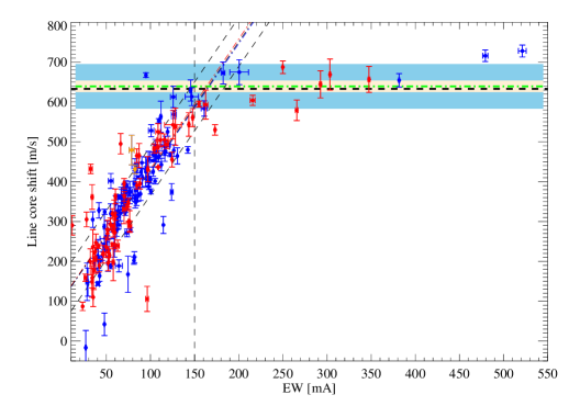
Figure 5: Line core shift of Fe i spectral lines, estimated using the recalibrated wavelengths $\lambda_{\rm nist}$ as reference laboratory wavelengths, measured on HARPS-LFC Moon spectra in the blue chip (blue dots) and in the red chip (red dots). Line core shifts of the two Fe ii lines are displayed as orange symbols. Blue, red, and black dashed-dotted lines show the linear fits of the blue, red, and all dots corresponding to the lines with EWs smaller then 170 mÅ. The horizontal black dashed line shows the theoretical solar gravitational redshift (GRS) measured on Earth, $v_{\rm GRS,theo}=633.10$ m s^-1. The green dashed-dotted line shows the mean line core shift, $v_{\rm GRS,obs}$, of the $N=15$ lines at EWs greater than 150 mÅ. The light blue and light yellow regions show the standard deviation, $\sigma_{\rm GRS,obs}$, and the $\sigma_{\rm GRS,obs}/\sqrt{N}$.

6 Solar gravitational redshift

We computed the mean line core shifts of each line of the sample of 257 Fe lines measured on the five HARPS-LFC spectra of the Moon. The uncertainties are computed as the standard deviation of the measurements. In order to remove outliers in the measurements among the line core shifts of the five spectra, we rejected all the lines with an line core shifts different from the mean by more than a factor of 1.5 times the standard deviation. We checked other threshold factors such as 2, 2.5, and 3 times the standard deviation, but we decided to remain in a restrictive position. This factor of 1.5 versus 2.0 or 3.0 does not have a significant implication (i.e. $\leq 5-10$ ${\rm m\;s^{-1}}$ difference) for the mean line core shift, but in some cases, it has an appreciable effect on the final uncertainty.

In Fig. 5, we display the mean line core shifts with respect to their equivalent widths. We identify 12 and 15 lines in the blue and red chips with uncertainties on line core shift between 50 and 100 ${\rm m\;s^{-1}}$ and with EWs smaller than 60 ${\rm m{\AA}}$, which were discarded from Fig. 5. Among a total of 230 lines, that is, 141 and 89 lines in the blue and red chips, respectively, a final sample of 188 lines are depicted in Fig. 5, with 116 and 72 in the blue and red, which have laboratory wavelengths flagged as A. In Table A.1, we provide the original wavelengths, $\lambda_{\rm lab}$, and the recalibrated wavelengths, $\lambda_{\rm nist}$ and $\lambda_{\rm ritz}$, together with other line parameters and with the observed line core shifts, $v_{\rm core,obs}$, of these 188 lines, computed as explained in Section 3. This line core shift uses as reference wavelength $\lambda_{\rm lab}$. Using the $\lambda_{\rm nist}$ and $\lambda_{\rm ritz}$ would lead to a greater line core shift by about 20 and 35 ${\rm m\;s^{-1}}$, respectively.

The measured line core shift, $v_{\rm core,obs}$, of these lines increases towards larger EWs up to about 170 ${\rm m{\AA}}$ and then stays roughly constant. As this increase seems to be linear, we fit the line core shifts versus EWs with linear functions for both the blue and the red lines and with all lines together and we find that this linear fits intersects the theoretical solar gravitational redshift at about 170 ${\rm m{\AA}}$. We fit line core shifts versus equivalent widths for lines weaker than 150 ${\rm m{\AA}}$. The standard deviation of the residuals of this fit is roughly 61 ${\rm m\;s^{-1}}$, whereas using the $\lambda_{\rm nist}$ and $\lambda_{\rm ritz}$ gives a standard deviation of the fit of 61 ${\rm m\;s^{-1}}$ and 67 ${\rm m\;s^{-1}}$, respectively. In Fig. 5, we depict the result using $\lambda_{\rm nist}$ as the reference laboratory wavelengths. The fit of lines weaker than 150 ${\rm m{\AA}}$ intersects the theoretical GRS at $\sim 165$ ${\rm m{\AA}}$and using the standard deviation of the fit gives an uncertainty of $\sim 15$ ${\rm m{\AA}}$. The observed line core shifts for lines stronger than approximately 150 ${\rm m{\AA}}$ stays roughly constant, reaching a similar value as the theoretical solar GRS.

Theory predicts that convective effects on the photospheric lines are less important as their cores are formed higher in the solar atmosphere. Lines with larger EWs, and therefore stronger lines, have their cores formed higher in the atmosphere. These observations seem to indicate that above a certain EW limit (see Fig. 5), the lines do not show any convective blue shift and, thus, their cores are only affected by the solar gravitational redshift. Therefore, we consider strong lines with EWs larger than 150 ${\rm m{\AA}}$ appropriate for observational measurements of the solar gravitational redshift. There are 15 strong lines with $150<$ EW[${\rm m{\AA}}$] $<550$, that is, 6 and 9 lines in blue and red chips, respectively. We computed the mean line core shift for these strong lines at $v_{\rm GRS,obs}=639\pm 14$ ${\rm m\;s^{-1}}$. The uncertainty is derived as the standard deviation of the measurements, $\sigma_{\rm GRS,obs}$, from the mean divided by the square root of the number of measurements, $N$, and thus, the final uncertainty as $\delta v_{\rm GRS,obs}=\sigma_{\rm GRS,obs}/\sqrt{N}$. This measurement is consistent with the theoretical value of the solar gravitational redshift, $v_{\rm GRS,theo}=633.1$ ${\rm m\;s^{-1}}$. As an observational test of the general theory of relativity (Einstein, 1916), it represents the most robust spectroscopic measurement of the gravitational redshift of the Sun.

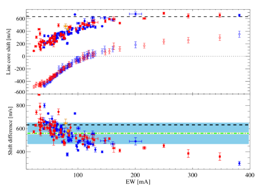
Figure 6: Top panel: Line core shift of Fe i spectral lines, estimated using the recalibrated wavelengths, $\lambda_{\rm nist}$, as reference laboratory wavelengths, measured on HARPS-LFC Moon spectra in the blue chip (blue dots) and in the red chip (red dots), and those measured on 3D hydrodynamical theoretical line profiles (open circles) for the same lines. Line core shifts of the two Fe ii lines are displayed as orange symbols. The dotted line shows the zero shift for reference. Bottom panel: Line core shift difference of the observed spectral lines and the theoretical line profiles. The black dashed line in both panels shows the theoretical solar GRS. The green dashed-dotted line shows the mean line core shift, $v_{\rm GRS,3D,lc}$, of the $N=144$ lines at $10<EW[$mÅ$]<400$. The light blue and light yellow regions show the standard deviation, $\sigma_{\rm GRS,3D,lc}$, and the $\sigma_{\rm GRS,3D,lc}/\sqrt{N}$.

In Fig. 6 we display both the observed and theoretical line core shifts of lines with $10<$ EW[${\rm m{\AA}}$] $<400$. A total of 144 lines is depicted, that is, 80 and 64 in the blue and red chips, respectively, with laboratory wavelengths flagged as A. Again, we chose the recalibrated wavelengths, $\lambda_{\rm nist},$ as reference wavelengths. The line core shift of the 3D profiles are estimated by linearly interpolating the line core shifts of the three line profiles in the observed EW according to the EW of the 3D profiles. The uncertainties on the line shifts of 3D profiles from different snapshots are estimated as the standard deviation of the line core shifts of the different snapshots divided by the square root of the number of snapshots, $N=20$. The uncertainty versus EW (and therefore line depth) increases progressively from 25 ${\rm m\;s^{-1}}$ at EW $=20$ ${\rm m{\AA}}$ to about 50 ${\rm m\;s^{-1}}$ at EW $=400$ ${\rm m{\AA}}$. The mean uncertainty is 31 ${\rm m\;s^{-1}}$.

The difference between the predicted line core (red) shift of the lines with the observed spectra of the Moon and the line core (mostly blue) shift measured in the 3D line profiles should also provide another observational measurement of the solar gravitational redshift. In the top panel of Fig. 6, we can see that both the observed and theoretical line core shifts increase towards larger EWs. Qualitatively the 3D line cores follow the same behaviour as the observed line cores. However, as seen in the bottom panel of Fig. 6, the velocity field of the 3D model atmosphere does not exactly reproduce the observations quantitatively, as the 3D line cores are more redshifted than the observed line cores as the lines are stronger than about 60 ${\rm m{\AA}}$. Stronger lines are more redshifted than expected, and at about 110 ${\rm m{\AA}}$, the line core shift becomes positive and continues to increase towards larger equivalent widths. This effect has been previously reported in the literature for both CO⁵BOLD and STAGGER models (e.g. Allende Prieto et al., 2009).

The cores of strong lines form at heights that can be influenced by the upper boundary of the 3D model. There must be some effects missing in the 3D model and, thus, subsequent spectral synthesis calculations, which lead to a decorrelation between velocity and temperature in the upper regions of the photosphere that would remove line shifts. Candidates are non-LTE effects and magnetic fields. While conducting non-LTE spectral syntheses for the many iron lines is beyond the scope of this paper, test calculations including magnetic fields in 3D models show that the presence of magnetic fields indeed reduces the redshifts of line cores. We could not obtain a quantitative correspondence. Moreover, magnetic fields that are strong enough to reduce the core shift of strong lines also reduce the shift of weak lines. Thus, magnetic field tend to suppress both negative and positive intrinsic line shifts both in weak and strong lines, respectively. A similar result has been found in Pereira et al. (2013), as seen in their Fig. 14 for lines weaker than 100 ${\rm m{\AA}}$. While the field geometry in local-box 3D models is somewhat arbitrary, it is difficult to envision a configuration that reduces the shift of strong lines while retaining the shift of weak lines. Non-LTE effects may be the reason for the mismatch. In 3D NLTE, the over-ionization of Fe i reduces line strengths changing the formation depth, in particular, low-excitation are significantly weakened, possibly affecting line shifts (Holzreuter & Solanki, 2013; Lind et al., 2017).

The difference between observed line core shifts and 3D line core shifts shows that weak lines with EWs smaller than 60 ${\rm m{\AA}}$ appear to show consistency with the solar GRS. However, the difference gets larger as we increase more and more the strengths of the lines. The mean shift difference between observed and 3D line cores is $v_{\rm GRS,3D,lc}=560\pm 8$ ${\rm m\;s^{-1}}$. The uncertainty is again derived as $\sigma_{\rm GRS,3D,lc}/\sqrt{N}$ with the standard deviation, $\sigma_{\rm GRS,3D,lc}$, and the number of lines, $N=144$ (see Fig. 6).

The line cores of 3D profiles do not exactly follow the same behaviour as the observed line cores, but 3D line profiles, as a whole, may do be shown to do so. We explored this possibility by computing global line shifts to the observed lines with the 3D profiles using our own automated code, as shown in Section 5.

In Fig. 7, we display global line shifts, estimated using the recalibrated wavelengths $\lambda_{\rm nist}$ for the reference laboratory wavelengths, as a function of the observed EW of the Fe lines. We discarded lines by visually inspecting the global line fits and by computing the reduced $\chi$ square, $\chi^{2}_{\nu}=\sum_{i=1}^{n}[(f_{i{\rm,obs}}-f_{i{\rm,3D}})/\sigma_{i}]^{2}/\nu$, where $i$ corresponds to each of the $n=11$ observed flux points, $f_{i{\rm,obs}}$, around the line core, with their uncertainties, $\sigma_{i}$, and the 3D profile flux values, $f_{i{\rm,3D}}$, and $\nu=n-m$ are the degrees of freedom and $m=3$ is the number of fitted parameters (see bottom-right panel of Fig. 4). As the good line fits, we adopt those with apparent good global line fits and reasonable line core fits, with $\chi_{\nu}^{2}<25$. We apply a 3-$\sigma$ clipping procedure on the global line shifts to remove five lines with shifts above 800 ${\rm m\;s^{-1}}$, thus leaving a final number of 97 lines with $10<$ EWs[${\rm m{\AA}}$] $<180$, 51 and 46 lines in the blue and red chips, respectively. We decided to restrict the upper boundary on EW of the global line fits to 180 ${\rm m{\AA}}$ to be able to compare the results with those of line core shifts. In addition, stronger lines are more difficult to fit globally since these lines are typically blended with other lines and a proper fit should include these weaker lines to be able to faithfully reproduce the line profiles.

The observed line core shifts, $v_{\rm core,obs,n}$, computed using the recalibrated wavelengths, $\lambda_{\rm nist}$, as reference laboratory wavelengths, the 3D line core shifts, $v_{\rm core,3D}$, and the global line shifts, $v_{\rm fit,3D,n}$, corrected using the recalibrated wavelengths $\lambda_{\rm nist}$ as reference laboratory wavelengths, of these 97 lines are provided in Table A.2 together with other line parameters. In Fig. 7, these global line shifts, $v_{\rm fit,3D,n}$, are distributed around the expected solar GRS. The mean shift of observed lines with respect to the 3D line profiles is $v_{\rm GRS,3D}=638\pm 6$ ${\rm m\;s^{-1}}$, in agreement with the theoretical value of the solar GRS. The uncertainty is again determined as $\sigma_{\rm GRS,3D}/\sqrt{N}$ with $N=97$ lines.

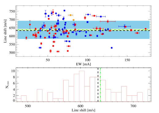
Figure 7: Top panel: Line shift from Fe i spectral lines, estimated using the recalibrated wavelengths, $\lambda_{\rm nist}$, as reference laboratory wavelengths, fitted on HARPS-LFC Moon spectra with 3D line profiles in the blue chip (blue dots) and in the red chip (red dots). Line shifts of the two Fe ii lines are displayed as orange symbols. The light blue and light yellow regions show the standard deviation, $\sigma_{\rm GRS,3D}$, and the $\sigma_{\rm GRS,3D}/\sqrt{N}$. Bottom panel: Histogram of the line shifts. The black dashed line shows the theoretical solar GRS. The green dashed-dotted line shows the mean line shift, $v_{\rm GRS,3D}$, of $N=97$ lines at $10<EW[$mÅ$]<180$.

7 Discussion and Conclusions

The analysis of high-quality HARPS spectra of the Moon calibrated with the laser frequency comb allows us to obtain an observational measurement of the solar GRS. We performed the analysis on an automated basis, using data reduction, wavelength calibration, continuum normalisation, and identification of lines and measurement of equivalent widths, line core shifts and global line shifts. There are uncertainties hidden in these process that certainly introduce some scatter in the measurements at the level of several tens of ${\rm m\;s^{-1}}$. We note the pixel size is $\sim 800$ ${\rm m\;s^{-1}}$ in the HARPS blue and red detectors. We are able to show a rather clear boundary in the equivalent widths of the lines, at $165\pm 15$ ${\rm m{\AA}}$, where lines with larger equivalent widths do not show any sign of convective shift. The 15 Fe lines with EWs larger than 150 ${\rm m{\AA}}$, are distributed around the theoretical value of solar GRS with a dispersion of 56 ${\rm m\;s^{-1}}$. The mean uncertainty on line core shift of these 15 lines is 23 ${\rm m\;s^{-1}}$, which is almost half of the dispersion of the measurements. This may be explained by the uncertainty on laboratory wavelengths at the level of $16-75$ ${\rm m\;s^{-1}}$ (Nave et al., 1994). The mean uncertainty on EW for these 15 Fe lines is 2.4 ${\rm m{\AA}}$. For the total number of 188 Fe lines, the mean uncertainty on line core shift is 19.2 ${\rm m\;s^{-1}}$, whereas mean uncertainty on EW is only 1.2 ${\rm m{\AA}}$.

The velocity field in the 3D model atmosphere of the Sun seems to reproduce quite well the observed behaviour of line core shifts, at least qualitatively, and quantitatively for weak lines with EW $<60$ ${\rm m{\AA}}$. On the other hand, the global line shift from the 3D profiles matching the observed profiles behaves better although there remains a dispersion in the measurements around the mean of about 73 ${\rm m\;s^{-1}}$ for the sub-sample of 102 Fe lines, and goes down to 55 ${\rm m\;s^{-1}}$ if we discard the five outliers by applying a $\sigma$ clipping procedure, leaving 97 Fe lines depicted in Fig. 7. The mean uncertainty on the global line shift that comes from the automated fitting procedure and computed as the standard deviation from the measurements of the five HARPS-LFC spectra is much smaller at 6 ${\rm m\;s^{-1}}$. However, the statistical uncertainty on the wavelength position of the average 3D profiles is a bit larger at about 30 ${\rm m\;s^{-1}}$. This may indicate that the dispersion around the theoretical value of solar GRS of 55 ${\rm m\;s^{-1}}$ may be indeed related to the uncertainty on the laboratory wavelengths. The recalibrated wavelengths, $\lambda_{\rm nist}$, do provide a slightly different result than the original laboratory wavelengths, $\lambda_{\rm lab}$, in Nave et al. (1994), shifting the result by +20 ${\rm m\;s^{-1}}$. Similarly, although the uncertainties on the recalibrated Ritz wavelengths estimated from the energy levels, $\lambda_{\rm ritz}$, are smaller than those of the original wavelengths, using the $\lambda_{\rm ritz}$ moves the result by +35 ${\rm m\;s^{-1}}$ and provides a larger dispersion. New laboratory experiments to improve the accuracy and revise the laboratory wavelengths of Fe i and other element species abundant in the visible solar spectrum appears necessary.

Assuming the recalibrated wavelengths, $\lambda_{\rm nist}$, as a laboratory reference, we have been able to achieve an observational measurements of the solar GRS of $v_{\rm GRS,3D}=638\pm 6$ ${\rm m\;s^{-1}}$ from the mean of observed global line shifts of 97 Fe lines with $10<$ EWs[${\rm m{\AA}}$] $<180$, and $v_{\rm GRS,obs}=639\pm 14$ ${\rm m\;s^{-1}}$ from the mean line core shift of 15 strong Fe lines with EW $>150$ ${\rm m{\AA}}$. Both measurements are in perfect agreement with the theoretical value of the solar gravitational redshift, $v_{\rm GRS,theo}=633.1$ ${\rm m\;s^{-1}}$, representing an observational test of the general theory of relativity (Einstein, 1911, 1916). At the same time, our observations point out the high quality, along with some limitations, in the current 3D modelling of the solar lines. New, high-quality spectra of the Moon taken with HARPS (Mayor et al., 2003), or at an even higher resolution with ESPRESSO (Pepe et al., 2014; González Hernández et al., 2018) and calibrated with the laser frequency comb in a wider spectral range, could provide a larger number of Fe lines that can be used to measure accurate line shifts (and, in fact, line bisectors) as diagnostics for understanding the structure and dynamics of the solar photosphere and for validating and improving 3D model atmospheres, in addition to serving as a tool for definitively probing solar gravitational redshift.