GRACE: Gradient Harmonized and Cascaded Labeling for Aspect-based Sentiment Analysis

Abstract

In this paper, we focus on the imbalance issue, which is rarely studied in aspect term extraction and aspect sentiment classification when regarding them as sequence labeling tasks. Besides, previous works usually ignore the interaction between aspect terms when labeling polarities. We propose a GRadient hArmonized and CascadEd labeling model (GRACE) to solve these problems. Specifically, a cascaded labeling module is developed to enhance the interchange between aspect terms and improve the attention of sentiment tokens when labeling sentiment polarities. The polarities sequence is designed to depend on the generated aspect terms labels. To alleviate the imbalance issue, we extend the gradient harmonized mechanism used in object detection to the aspect-based sentiment analysis by adjusting the weight of each label dynamically. The proposed GRACE adopts a post-pretraining BERT as its backbone. Experimental results demonstrate that the proposed model achieves consistency improvement on multiple benchmark datasets and generates state-of-the-art results.

1 Introduction

Aspect terms extraction (ATE) and aspect sentiment classification (ASC) are two fundamental, fine-grained subtasks in aspect-based sentiment analysis (ABSA). ATE is the task of extracting the aspect terms (or attributes) of an entity upon which opinions have been expressed, and ASC is the task of identifying the polarities expressed on these extracted terms in the opinion text Hu and Liu (2004). Consider the example in Figure 1, which contains comments that people expressed about the aspect terms “operating system” and “keyboard”, and their polarities are all positive.

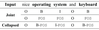
Figure 1: Joint and Collapsed labeling approaches on aspect terms and their polarities. POS means positive.

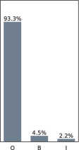
(a) Label statistics

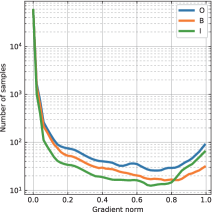
(b) Gradient statistics

Figure 2: Label statistics and gradient distribution on the laptop dataset of SemEval-14. The y-axis in (b) uses a log scale.

To better satisfy the practical applications, the aspect term-polarity co-extraction, which solves ATE and ASC simultaneously, receives much attention in recent years Li et al. (2019b); Luo et al. (2019b); Hu et al. (2019); Wan et al. (2020). A big challenge of the aspect term-polarity co-extraction in a unified model is that ATE and ASC belong to different tasks: ATE is usually a sequence labeling task, and ASC is usually a classification task. Previous works usually transform the ASC task into sequence labeling. Thus the ATE and ASC have the same formulation.

There are two approaches of sequence labeling on the aspect term-polarity co-extraction. As shown in Figure 1, one is the joint approach, and the other is the collapsed approach. The preceding one jointly labels each sentence with two different tag sets: aspect term tags and polarity tags. The subsequent one uses collapsed labels as the tags set, e.g., “B-POS” and “I-POS”, in which each tag indicates the aspect term boundary and its polarity. Except for the joint and collapsed approaches, a pipelined approach first labels the given sentence using aspect term tags, e.g., “B” and “I” (the beginning and inside of an aspect term), and then feeds the aspect terms into a classifier to obtain their corresponding polarities.

Several related works have been published in these approaches. Mitchell et al. (2013) and Zhang et al. (2015) found that the joint and collapsed approaches are superior to the pipelined approach on named entities and their sentiments co-extraction. Li et al. (2019b) proposed a unified model with the collapsed approach to do aspect term-polarity co-extraction. Hu et al. (2019) solved this task with a pipelined approach. Luo et al. (2019b) adopted the joint approach to do such a co-extraction. We follow the joint approach in this paper, and believe that it has a more apparent of responsibilities than the collapsed approach through learning parallel sequence labels.

However, previous works on the joint approach usually ignore the interaction between aspect terms when labeling polarities. Such an interaction is useful in identifying the polarity. As an instance, in Figure 1, if “operating system” is positive, “keyboard” should be positive due to these two aspect terms are connected by coordinating conjunction “and”. Besides, almost all of previous works do not concern the imbalance of labels in such sequence labeling tasks. As shown in 2a, the number of ‘O’ labels is much larger than that of ‘B’ and ‘I’, which tends to dominant the training loss. Moreover, we find the same gradient phenomenon as Li et al. (2019a) in the sequence labeling task. As shown in Figure 2b, most of the labels own low gradients, which have a significant impact on the global gradient due to their large number.

Considering the above issues, we propose a GRadient hArmonized and CascadEd labeling model (GRACE) in this paper. The proposed GRACE is shown in Figure 3. Unlike previous works, GRACE is a cascaded labeling model, which uses the generated aspect term labels to enhance the polarity labeling in a unified framework. Specifically, we use two encoder modules shared with lower layers to extract representation. One encoder module is for ATE, and the other is for ASC after giving the aspect term labels generated by the preceding encoder. Thus, the GRACE could consider the interaction between aspect terms in the ASC module through a stacked Multi-Head Attention Vaswani et al. (2017). Besides, we extend a gradient harmonized loss to address the imbalance labels in the model training phase.

Our contributions are summarized as follows:

• A novel framework GRACE is proposed to address the aspect term-polarity co-extraction problem in an end-to-end fashion. It utilizes a cascaded labeling approach to consider the interaction between aspect terms when labeling their sentiment tags.

• The imbalance issue of labels is considered, and a gradient harmonized strategy is extended to alleviate it. We also use virtual adversarial training and post-training on domain datasets to improve co-extraction performance.

In the following, we describe the proposed framework GRACE in Section 2. The experiments are conducted in Section 3, followed by the related work in Section 4. Finally, we conclude the paper in Section 5.

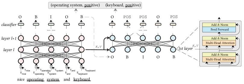
Figure 3: The main structure of our GRACE. It is a cascaded labeling architecture, which means that the generated aspect term labels [O,B,I,O,B] are fed to the right part as key $K$ and value $V$ to generate sentiment labels [O,POS,POS,O,POS]. The perturbed embeddings $r_{\cdot}$ is added to the Token embeddings $\mathit{E}_{\cdot}$.

2 Model

An overview of GRACE is given in Figure 3. It is comprised of two modules with the shared shallow layers: one is for ATE, and the other is for ASC. We will first formulate the co-extraction problem and then describe the framework in detail in this section.

2.1 Problem Statement

This paper deals with aspect term-polarity co-extraction, in which the aspect terms are explicitly mentioned in the text. We solve it as two sequence labeling tasks. Formally, given a review sentence $S$ with $n$ words from a particular domain, denoted by $S=\{w_{i}|i=1,\dots,n\}$. For each word $w_{i}$, the objective of our task is to assign a tag $t^{e}_{i}\in T^{e}$, and a tag $t^{c}_{i}\in T^{c}$ to it, where $T^{e}=\{$B, I, O$\}$ and $T^{c}=\{$POS, NEU, NEG, CON, O$\}$. The tags ‘B’, ‘I’ and ‘O’ in $T^{e}$ stand for the beginning, the inside of an aspect term, and other words, respectively. The tags POS, NEU, NEG, and CON indicate polarity categories: positive, neutral, negative, and conflict, respectively . The tag ‘O’ in $T^{c}$ means other words like that in $T^{e}$. Figure 1 shows a labeling example of the joint and collapsed approaches.

2.2 GRACE: Gradient Harmonized and Cascaded Model

We focus on the joint labeling approach in the paper. As shown in Figure 3, the proposed GRACE contains two branches with the shared shallow layers. In order to benefit from the pretrained model, we use the BERT-Base as our backbone. Then the representation $\mathbf{H}_{e}$ of ATE can be generated on the pretrained BERT:

$$\mathbf{H}^{[1:L]}=\text{BERT}(S),$$ (1)

$$\mathbf{H}_{e}=\mathbf{H}^{L},$$ (2)

where $\mathbf{H}^{[1:L]}$ denotes the representation of each layer of BERT. It varies from the 1st layer to the $L$-th layer. $L$ is the max layer of BERT, e.g., 12 in BERT-Base. $\mathbf{H}_{e}\in\mathbb{R}^{(\hat{n}+2)\times h}$ is the representation $\mathbf{H}^{L}$ belonging to the last layer, in which two extra embeddings belong to special tokens [CLS] and [SEP], and the labels of them are set to ‘O’ in the experiments. $h$ is the hidden size, $\hat{n}$ is the length of $S$ after tokenizing by the wordpiece vocabulary.

Different layers of BERT capture different levels of information, e.g., phrase-level information in the lower layers and linguistic information in intermediate layers Jawahar et al. (2019). The higher layers are usually task-related. Thus, a shared BERT between ATE and ASC tasks is the right choice. We extract the representation $\mathbf{H}_{c}$ for ASC task from the $l$-th layer of BERT:

$$\mathbf{H}_{c}=\mathbf{H}^{l}.$$ (3)

Thus, $\mathbf{H}^{[l+1:L]}$ is task-specific for ATE. An extreme state is $l=L$, where all layers are shared across both tasks. We omit an exhaustive description of BERT and refer readers to Devlin et al. (2019) for more details.

Cascaded Labeling We can do sequence labeling on the $\mathbf{H}_{e}$ and $\mathbf{H}_{c}$ directly. However, it is not a customized feature for ASC. Conversely, ASC may decline the ATE performance. One reason is the difference between ATE and ASC. The polarity of an aspect term usually does not come from the term itself. For example, the polarity of aspect term “operating system” in Figure 1 comes from the adjective “nice”. When labeling the “operating system”, the model needs to point to the “nice”. The other reason is the interaction between aspect terms is ignored when labeling their sentiment labels. For example, the “operating system” and “keyboard” are connected by coordinating conjunction “and”. If “operating system” is positive, “keyboard” should be positive, too.

Thus, we propose the cascaded labeling approach, which uses the generated aspect terms sequence as the input to generate the sentiment sequence. As shown in Figure 3, the $\mathbf{H}_{c}$ is fed to a new Transformer-Decoder Vaswani et al. (2017) as key $K$ and value $V$ to generate a new aspect sentiment representation $\mathbf{G}_{c}$:

$$\mathbf{G}_{c}=\text{Transformer-Decoder}(\mathbf{H}_{c},Q),$$ (4)

where $Q$ represents the aspect term labels generated by the ATE module (ground-truth labels in the training phase). The vocab size is $|T^{e}|$ in the word embedding of the Transformer-Decoder.

Note that the Transformer-Decoder here is not the same as the original transformer decoder. The difference is that we use Multi-Head Attention instead of Masked Multi-Head Attention as the first sub-layer because the ASC is not an autoregressive task and does not need to predict the output sequence one element at a time.

Gradient Harmonized Loss The cross entropy is used to train the model:

$$p^{\tau}=\textrm{softmax}(\mathbf{M}_{\tau}\mathbf{w}_{\tau}),$$ (5)

$$\mathcal{L}_{\tau}=-\frac{1}{n}\sum_{i=1}^{n}\left(\mathbb{I}\left(t_{i}^{\tau}\right)\left(\text{log}\left(p^{\tau}_{i}\right)\right)^{\top}\right),$$ (6)

where $\tau\in\{e,c\}$, $\mathbf{M}=\mathbf{H}$ if $\tau$ is $e$, and $\mathbf{M}=\mathbf{G}$ if $\tau$ is $c$, $\mathbb{I}(t_{i}^{\tau})$ means the one-hot vector of $t_{i}^{\tau}\in T^{\tau}$, $\mathbf{w}_{\tau}$ is a trainable weight matrix.

Then, the losses from both tasks are constructed as the joint loss of the entire model:

$$\mathcal{J}(\Theta)=\mathcal{L}_{e}+\mathcal{L}_{c},$$ (7)

where $\mathcal{L}_{e}$ and $\mathcal{L}_{c}$ denote the loss for aspect term and polarity, respectively. $\Theta$ represents the model parameters containing all trainable weight matrices and bias vectors.

However, there are two well-known disharmonies to affect the performance through the optimization of the above losses. The first one is the imbalance between positive and negative examples, and the other one is the imbalance between easy and hard examples Li et al. (2019a). Specifically, there exists the imbalance between each label in our labeling task. As shown in Figure 2a, the label ‘O’ occupies a tremendous rate than other labels. According to the work from Li et al. (2019a), the easy and hard attributes of labels can be represented by the norm of gradient $g$:

$$g=\left|\frac{\partial\mathcal{L}}{\partial z}\right|=|p-\hat{t}|,$$ (8)

where $\hat{t}$ is the ground-truth with value 0 or 1, $p$ is the score calculated by a softmax operation, $z$ is the logit output of a model, $\mathcal{L}$ is the cross entropy. E.g., $z=\mathbf{M}_{\tau}\mathbf{w}_{\tau}$ and $p$ in Eq. (5), and $\mathcal{L}$ in Eq. (6).

Figure 2b shows the statistic of labels w.r.t gradient norm $g$. Most of the labels own low gradients, which have a significant impact on the global gradient due to their large number. A strategy is to decrease the weight of loss from these labels.

We rewrite the Eq. (6) following GHM-C, which used in object detection Li et al. (2019a), as follows:

$$\mathcal{L}_{\tau}=-\frac{1}{n}\sum_{i=1}^{n}\left(\beta_{t_{i}^{\tau}}\big{(}\mathbb{I}\left(t_{i}^{\tau}\right)\left(\text{log}\left(p^{\tau}_{i}\right)\right)^{\top}\big{)}\right),$$ (9)

$$\beta_{t_{i}^{\tau}}=\frac{N^{\tau}}{\rho\left(g_{t_{i}^{\tau}}\right)},$$ (10)

where $g_{t_{i}^{\tau}}$ is the gradient norm of $t_{i}^{\tau}$ calculated by Eq. (8), $N^{\tau}$ is the total number of labels, $\rho(g)$ is gradient density:

$$\rho(g)=\frac{1}{l_{\epsilon}(g)}\sum_{k=1}^{N^{\tau}}\delta_{\epsilon}\left(g_{k},g\right),$$ (11)

where $\delta_{\epsilon}(x,y)$ is 1 if $y-\frac{\epsilon}{2}\leq x<y+\frac{\epsilon}{2}$ otherwise 0. The $\rho(g)$ denotes the number of labels lying in the region centered at $g$ with a length of $\epsilon$ and normalized by the valid length $l_{\epsilon}(g)=\min\left(g+\frac{\epsilon}{2},1\right)-\max\left(g-\frac{\epsilon}{2},0\right)$ of the region.

The calculation of $\beta_{t_{i}^{\tau}}$ will use the unit region to reduce complexity. Specifically, the gradient norm $g$ will put into $m={1}/{\epsilon}$ unit regions. For the $j$-th unit region $u_{j}=\big{[}j\epsilon-\epsilon,j\epsilon\big{)}$, the gradient density can be approximated as:

$$\hat{\rho}(g)=U_{ind(g)}/{\epsilon}=mU_{ind(g)},$$ (12)

where $U_{j}$ denotes the number of labels lying in $u_{j}$, $ind(g)=\kappa$ s.t. $(\kappa-1)\epsilon\leq g<\kappa\epsilon$ is the index of the unit region in which $g$ lies.

The calculation of $\hat{\rho}(g)$ assumpts that the examples lying in the same unit region share the same gradient density. So it can be calculated by the algorithm of histogram statistics.

A further reasonable manner is to statistics $U_{j}^{(t)}$ in the $t$-th iteration to reduce the complexity of $U_{j}$’s statistic cross the dataset, and uses $A_{j}^{(t)}$ to approximate the real $U_{j}$ as follows:

$$A_{j}^{(t)}=\alpha A_{j}^{(t-1)}+(1-\alpha)U_{j}^{(t)},$$ (13)

where $\alpha$ is a momentum parameter. Thus, the $\hat{\rho}(g)$ is updated by:

$$\hat{\rho}(g)={A_{ind(g)}}/{\epsilon}=mA_{ind(g)},$$ (14)

Virtual Adversarial Training To make the model more robust to adversarial noise, we utilize the virtual adversarial training (VAT) used in Miyato et al. (2016) to make small perturbations $r$ to the input Token Embedding $E$ when training model. The additional loss is as follows:

$$E^{*}=E+r,$$ (15)

$$\mathcal{L}_{\mathrm{VAT}}\!=\!\frac{1}{n}\!\!\sum_{i=1}^{n}\!\!D_{\mathrm{KL}}\big{(}p(\cdot|E;\!\Theta)\|p\left(\cdot|E^{*};\!\Theta\right)\big{)},$$ (16)

the adversarial perturbation $r$ is calculated by:

$$E^{\prime}=E+\xi d,$$ (17)

$$g=\nabla_{E^{\prime}}D_{\mathrm{KL}}\left(p\big{(}\cdot|E;\hat{\Theta}\big{)}\|p\big{(}\cdot|E^{\prime};\hat{\Theta}\big{)}\right),$$ (18)

$$r=\epsilon g/\left\|g\right\|_{2},$$ (19)

where $\epsilon$ and $\xi$ are hyperparameters, $d$ is sampled from normal distribution $\mathcal{N}(0,I)$, $\hat{\Theta}$ is a constant set to the current parameters $\Theta$, $D_{\mathrm{KL}}(\cdot\|\cdot)$ is the KL divergence, $p(\cdot|\cdot)$ is the model conditional probability.

On the whole, the total loss of the proposed GRACE is:

$$\mathcal{J}(\Theta)=\mathcal{L}_{e}+\mathcal{L}_{c}+\mathcal{L}_{\mathrm{VAT}},$$ (20)

where $\mathcal{L}_{e}$ and $\mathcal{L}_{c}$ are calculated by Eq. (9), denote the loss for aspect term and polarity, respectively. $\mathcal{L}_{\mathrm{VAT}}$ denotes the VAT loss, calculated by Eq. (16).

Consistent Polarity Label A question when regarding sentiment classification as polarity sequence labeling is that the generated sequence labels are not always consistent. For instance, the polarity labels may be ‘POS NEG’ for the aspect term ‘operating system’. To solve this problem, we design a strategy on the representation of tokens within the same aspect term. To the generated sequence labels of ASC, we first get the boundaries of aspect terms according to the meaning of the label, e.g., the boundary of the labels ‘O B I O B’ in Figure 3 is $\{[1,2),[2,4),[2,4),[4,5),[5,6)\}$, in which the element $[b_{ind},e_{ind})$ means begin index (inclusive) and end index (exclusive). Then the aspect sentiment representation $\mathbf{G}_{c}$, and the classification is calculated as follows:

$$g_{i}=\max(\mathbf{G}_{c}[b_{ind}:e_{ind}]),$$ (21)

$$h_{i}=f(g_{i}\mathbf{w}_{h}),$$ (22)

where $\mathbf{G}_{c}[b_{ind}:e_{ind}]$ is a snippet of $\mathbf{G}_{c}$ from $b_{ind}$ to $e_{ind}$ (exclusive), $\max$ is a max-pooling operator along with the sequence dimension. $\mathbf{w}_{h}$ is a trainable weight matrix. $f(\cdot)$ is the ReLU function. We use $h_{i}$ to calculate loss as Eq. (5) and Eq. (9). It is a consistent strategy to generate sentiment labels, although it cannot improve the performance in our preliminary experiments.

3 Experiments

3.1 Datasets

Datasets	#POS	#NEU	#NEG	#CON
$\mathbb{D}_{\text{L}}$	1,313	619	963	58
$\mathbb{D}_{\text{R}}$	4,878	937	1,751	102
- $\mathbb{D}_{\text{R-14}}$	2,868	820	977	102
- $\mathbb{D}_{\text{R-15}}$	1,222	62	451	0
- $\mathbb{D}_{\text{R-16}}$	1,676	93	581	0
$\mathbb{D}_{\text{T}}$	698	2,254	271	0

Table 1: Dataset statistics. $\mathbb{D}_{\text{L}}$, $\mathbb{D}_{\text{R}}$, and $\mathbb{D}_{\text{T}}$ denote laptop, restaurant, and twitter datasets, respectively. #POS, #NEU, #NEG, and #CON refer to the number of positive, neutral, negative, and conflict polarity categories, respectively.

We evaluate the proposed model on three benchmark sentiment analysis datasets, two of which come from the SemEval challenges, and the last comes from an English Twitter dataset, as shown in Table 1. $\mathbb{D}_{\text{L}}$ contains laptop reviews from SemEval 2014 Pontiki et al. (2014), and $\mathbb{D}_{\text{R}}$ are restaurant reviews merged from SemEval 2014 ($\mathbb{D}_{\text{R-14}}$), SemEval 2015 ($\mathbb{D}_{\text{R-15}}$) Pontiki et al. (2015), and SemEval 2016 ($\mathbb{D}_{\text{R-16}}$) Pontiki et al. (2016). We keep the official data division of these datasets for the training set, validation set, and testing set. The reported results of $\mathbb{D}_{\text{L}}$ and $\mathbb{D}_{\text{R}}$ are average scores of 5 runs. $\mathbb{D}_{\text{T}}$ consists of English tweets. Due to a lack of standard train-test split, we report the ten-fold cross-validation results of $\mathbb{D}_{\text{T}}$ as done in Li et al. (2019b); Luo et al. (2019b). The evaluation metrics are precision (P), recall (R), and F1 score based on the exact match of aspect term and its polarity.

3.2 Post-training

Domain knowledge is proved useful for domain-specific tasks Xu et al. (2019); Luo et al. (2019b). In this paper, we adopt Amazon reviews  and Yelp reviews , which are in-domain corpora for laptop and restaurant, respectively, to do a post-training on uncased BERT-Base for our tasks. The Amazon review dataset contains 142.8M reviews, and the Yelp review dataset contains 2.2M restaurant reviews. We combine all these reviews to finish our post-training. The maximum length of post-training is set to 320. The batch size is 4,096 for BERT-Base with gradient accumulation (every 32 steps). The BERT-Base is implemented base on the transformers library with Pytorch . The mask strategy is Whole Word Masking (WWM), the same as the official BERT . We use Adam optimizer and set the learning rate to be 5e-5 with 10% warmup steps. Our pretrained model is carried out 10 epochs on 8 NVIDIA Tesla V100 GPU. We use fp16 to speed up training and to reduce memory usage. The pre-training process takes more than 5 days.

3.3 Settings

During fine-tuning on ATE and ASC tasks, the optimizer is Adam with 10% warmup steps. A two-stage training strategy is utilized in our cascaded labeling model. In the first stage, we first fine-tune the ATE part initialized with the post-trained BERT weights. The learning rate is set to 3e-5 with 32 batch size, and running 5 epochs without virtual adversarial training. Then we plus virtual adversarial to continue to fine-tune 1 epoch for $\mathbb{D}_{\text{L}}$ and 3 epochs for other datasets with learning rate 1e-5. In the second stage, we fine-tune both ATE and ASC modules initialized with the weights from the first stage. The ASC decoder is initialized with the last corresponding layers of the ATE module. The learning rate is set to 3e-5 for the ASC part and 3e-6 for the ATE part with 32 batch size, and running 10 epochs. The maximum length is set to 128 on all datasets. $\epsilon$ in Eq. (11) is 24, and the momentum parameter $\alpha$ in Eq. (13) is 0.75. $\xi$ in Eq. (17) is set to 1e-6, and $\epsilon$ in Eq. (19) is set to 2. We set the shared layers $l=9$, and the number of transformer layers for ASC to 2. All the above hyper-parameters are tuned on the validation set of $\mathbb{D}_{\text{L}}$ and $\mathbb{D}_{\text{R}}$. We implement our GRACE using the same library as post-training, and all computations are done on NVIDIA Tesla V100 GPU.

Model	$\mathbb{D}_{\text{L}}$			$\mathbb{D}_{\text{R}}$			$\mathbb{D}_{\text{T}}$
	P	R	F1	P	R	F1	P	R	F1
E2E-TBSA	61.27	54.89	57.90	68.64	71.01	69.80	53.08	43.56	48.01
DOER	61.43	59.31	60.35	80.32	66.54	72.78	55.54	47.79	51.37
SPANBase	66.19	58.68	62.21	71.22	71.91	71.57	60.92	52.24	56.21
SPANLarge	69.46	66.72	68.06	76.14	73.74	74.92	60.72	55.02	57.69
BERT-E2E-ABSA	61.88	60.47	61.12	72.92	76.72	74.72	57.63	54.47	55.94
GRACE	72.38	69.12	70.71	75.95	80.31	78.07	58.36	58.22	58.28
-w/o GHL	68.64	65.90	67.24	75.16	78.66	76.87	55.53	55.62	55.56
-w/o VAT	72.28	67.67	69.89	75.75	79.97	77.80	56.81	58.41	57.58
-w/o PTR	66.39	61.70	63.96	73.28	76.53	74.87	57.26	58.86	58.04

Table 2: Comparison results (%) for aspect term-polarity pair extraction on three benchmark datasets. State-of-the-art results are marked in bold. ‘-w/o GHL’ means GRACE without gradient harmonized loss, ‘-w/o VAT’ is GRACE without virtual adversarial training, and ‘-w/o PTR’ is GRACE without post-training on BERT-Base.

Model	$\mathbb{D}_{\text{L}}$	$\mathbb{D}_{\text{R-14}}$	$\mathbb{D}_{\text{R-15}}$	$\mathbb{D}_{\text{R-16}}$
IMN	58.37	69.54	59.18	-
DREGCN	63.04	72.60	62.37	-
WHW	62.34	71.95	65.79	71.73
TAS-BERT	-	-	66.11	75.68
IKTN-BERT	62.34	71.75	62.33	-
DHGNN	59.61	68.91	58.37	-
RACL-BERT	63.40	75.42	66.05	-
GRACE	70.71	77.26	68.16	76.49
-w/o GHL	67.24	75.83	66.73	75.09
-w/o VAT	69.89	77.16	67.75	76.03
-w/o PTR	63.96	71.56	59.82	66.95

Table 3: Comparison results of F1 score (%) for aspect term-polarity pair extraction on four benchmark datasets. ‘-’ denotes unreported results. ‘-w/o GHL’, ‘-w/o VAT’, and ‘-w/o PTR’ have the same meaning as which in Table 2.

3.4 Baseline Methods

We compare our model  with the following models:

E2E-TBSA Li et al. (2019b) is an end-to-end model of the collapsed approach proposed to address ATE and ASC simultaneously.

DOER Luo et al. (2019b) employs a cross-shared unit to train the ATE and ASC jointly.

SPAN Hu et al. (2019) is a pipeline approach built on BERT-Large (SPAN_Large) to solve aspect term-sentiment pairs extraction. We implement its BERT-Base version (SPAN_Base) using the available code .

BERT-E2E-ABSA Li et al. (2019c) is a BERT-based benchmark for aspect term-sentiment pairs extraction. We use the BERT+GRU for $\mathbb{D}_{\text{L}}$ and BERT+SAN for $\mathbb{D}_{\text{R}}$ as our baselines due to their best-reported performance. Besides, we produce the results on $\mathbb{D}_{\text{T}}$ with BERT+SAN keeping the settings the same as on $\mathbb{D}_{\text{R}}$ .

We compare our model with the above baselines on $\mathbb{D}_{\text{L}}$, $\mathbb{D}_{\text{R}}$, and $\mathbb{D}_{\text{T}}$, and compare it with the following baselines on $\mathbb{D}_{\text{L}}$, $\mathbb{D}_{\text{R-14}}$, $\mathbb{D}_{\text{R-15}}$, and $\mathbb{D}_{\text{R-16}}$ because of the common datasets reported by the official implementation.

IMN He et al. (2019) uses an interactive architecture with multi-task learning for end-to-end ABSA tasks. It contains aspect term and opinion term extraction besides aspect-level sentiment classification.

DREGCN Liang et al. (2020a) designs a dependency syntactic knowledge augmented interactive architecture with multi-task learning for end-to-end ABSA. DREGCN is short for the official DREGCN+CNN+BERT due to its better performance.

WHW Peng et al. (2020) develops a two-stage framework to address aspect term extraction, aspect sentiment classification, and opinion extraction.

TAS-BERT Wan et al. (2020) proposes a method based on BERT-Base that can capture the dependence on both aspect terms and categories for sentiment prediction. TAS-BERT is short for the official TAS-BERT-SW-BIO-CRF due to its better performance.

IKTN+BERT Liang et al. (2020b) discriminately transfers the document-level linguistic knowledge to aspect term, opinion term extraction, and aspect-level sentiment classification.

DHGNN Liu et al. (2020) presents a dynamic heterogeneous graph to model the aspect extraction and sentiment detection explicitly jointly.

RACL-BERT Chen and Qian (2020) is built on BERT-Large and allows the aspect term extraction, opinion term extraction, and aspect-level sentiment classification to work coordinately via the multi-task learning and relation propagation mechanisms in a stacked multi-layer network.

3.5 Results and Analysis

Comparison Results. The comparison results are shown in Table 2 and Table 3 because different baselines officially report on different datasets. Overall, our proposed GRACE consistently obtains the best F1 score across all datasets and significantly outperforms the strongest baselines in most cases on aspect term-polarity co-extraction. Compared to the state-of-the-art pipeline approach, the GRACE outperforms SPAN_Base by 8.50%, 6.50%, and 2.07% on $\mathbb{D}_{\text{L}}$, $\mathbb{D}_{\text{R}}$, and $\mathbb{D}_{\text{T}}$, respectively. Even comparing to SPAN_Large built on 24-layers BERT-Large, the improvements are still 2.65%, 3.15%, and 0.59% on $\mathbb{D}_{\text{L}}$, $\mathbb{D}_{\text{R}}$, and $\mathbb{D}_{\text{T}}$, respectively. It indicates that a carefully-designed joint model has capable of achieving better performance than pipeline approaches on our task. Compared to other multi-task models containing additional information, e.g., opinion terms and aspect term categories, the GRACE achieves absolute gains over the IMN, WHW, TAS-BERT, IKTN+BERT, and RACL-BERT at least by 7.31%, 1.84%, 2.05%, and 0.81% on $\mathbb{D}_{\text{L}}$, $\mathbb{D}_{\text{R-14}}$, $\mathbb{D}_{\text{R-15}}$, $\mathbb{D}_{\text{R-16}}$, respectively. It suggests that GRACE can extend to more tasks of ABSA.

Ablation Study. To study the effectiveness of the gradient harmonized loss (GHL), VAT, and post-pretraining, we conduct ablation experiments on each of them. The results are shown in the second block in Table 2 and Table 3. We can see that the scores drop more seriously without GHL comparing to that without VAT. It points out that GRACE can benefit more from the gradient harmonized loss than VAT, and alleviate the imbalance issue of labels is more important to the sequence labeling. The drop of scores without post-training is the worst on all laptop and restaurant datasets, which indicates that the domain-specific knowledge can improve the task-related datasets massively.

Model	$\mathbb{D}_{\text{L}}$	$\mathbb{D}_{\text{R}}$	$\mathbb{D}_{\text{T}}$
DE-CNN	81.26	78.98	63.23
DOER	82.61	81.06	71.35
SPANLarge	83.35	82.38	75.28
BERT-PT	84.26	-	-
BERT-PT-AUG	85.33	-	-
BAT	85.57	-	-
GRACE	87.93	85.45	75.73
-w/o ASC	87.45	84.49	75.52

Table 4: F1 score (%) comparison for aspect term extraction. ‘-’ denotes unreported results. ‘-w/o ASC’ means training without the ASC branch.

Sentence	BASE	GRACE w/o GHL	GRACE
I used [windows XP]${}_{\texttt{NEU}}$, [windows Vista]${}_{\texttt{NEU}}$, and [Windows 7]${}_{\texttt{NEU}}$ extensively.	[windows XP]${}_{\texttt{POS}}$ (✗)	[windows XP]${}_{\texttt{NEU}}$	[windows XP]${}_{\texttt{NEU}}$
	[windows Vista]${}_{\texttt{NEU}}$	[windows Vista]${}_{\texttt{NEU}}$	[windows Vista]${}_{\texttt{NEU}}$
	[Windows 7]${}_{\texttt{NEU}}$	[Windows 7]${}_{\texttt{NEU}}$	[Windows 7]${}_{\texttt{NEU}}$
User upgradeable [RAM]${}_{\texttt{POS}}$ and [HDD]${}_{\texttt{POS}}$.	[RAM]${}_{\texttt{POS}}$	[RAM]${}_{\texttt{POS}}$	[RAM]${}_{\texttt{POS}}$
	[HDD]${}_{\texttt{NEU}}$ (✗)	[HDD]${}_{\texttt{POS}}$	[HDD]${}_{\texttt{POS}}$
Although somewhat loud, the [noise]${}_{\texttt{CON}}$ was minimally intrusive.	[noise]${}_{\texttt{POS}}$ (✗)	[noise]${}_{\texttt{POS}}$ (✗)	[noise]${}_{\texttt{CON}}$
The [atmosphere]${}_{\texttt{CON}}$ was nice but it was a little too dark.	[atmosphere]${}_{\texttt{POS}}$ (✗)	[atmosphere]${}_{\texttt{POS}}$ (✗)	[atmosphere]${}_{\texttt{CON}}$

Table 5: Case analysis on BASE, GRACE w/o GHL, and GRACE. ✗ means wrong prediction.

Results on ATE. As an extra output of the proposed GRACE, we also compare ATE results with state-of-the-art baselines. DE-CNN Xu et al. (2018) adopts CNN training on general purpose embeddings domain specific embeddings to finish ATE. BERT-PT Xu et al. (2019) post-trains BERT’s weights using in-domain review datasets and MRC dataset. It is implemented based on BERT-Base. BERT-PT-AUG Li et al. (2020) is an improvement version of BERT-PT with a controllable data augmentation approach. BAT Karimi et al. (2020) is a BERT adversarial training model. The results of the ATE are shown in Table 4. Our GRACE achieves state-of-the-art results over baselines. The lower scores of GRACE without the ASC branch indicate that the ASC task could enhance the ATE.

Results on Cascaded Labeling. To verify the effectiveness of our cascaded labeling strategy, as a particular case of the GRACE, we set the shared layers $l=12$ and set the number of transformer layers for ASC to 0, and refer it as BASE. Thus, there is no generated aspect term label from ATE branch when training the ASC branch. The F1 scores of BASE are 68.35% and 76.76% on $\mathbb{D}_{\text{L}}$ and $\mathbb{D}_{\text{R}}$, respectively. The results are lower than 70.71% and 78.07% of GRACE on the same datasets. This fact indicates that considering the interaction between aspect terms and paying more attention to other tokens are benefit to the sentiment labeling.

Case Study. Table 5 shows some examples of BASE, GRACE without gradient harmonized loss (w/o GHL), and GRACE sampled from $\mathbb{D}_{\text{L}}$ and $\mathbb{D}_{\text{R}}$. As observed in the first two examples, the GRACE incorrectly predicts both aspect terms and their sentiments. Comparing with the BASE, we believe the cascaded labeling strategy can make an interaction between aspect terms within a sentence, which enhances the judgment of sentiment labels. The last two rows indicate that GRACE can get correct results, even the CON is minimal. The reason is not only the more comprehensive information proved by cascaded labeling strategy but also the balance of labels given by gradient harmonized loss.

4 Related Work

Aspect term extraction and aspect sentiment classification are two major topics of aspect-based sentiment analysis. Many researchers have studied each of them for a long time. For the ATE task, unsupervised methods such as frequent pattern mining Hu and Liu (2004), rule-based approach Qiu et al. (2011); Liu et al. (2015), topic modeling He et al. (2011); Chen et al. (2014), and supervised methods such as sequence labeling based models Wang et al. (2016a); Yin et al. (2016); Xu et al. (2018); Li et al. (2018); Luo et al. (2019a); Ma et al. (2019) are two main directions. For the ASC task, the relation or position between the aspect terms and the surrounding context words are usually used Tang et al. (2016); Laddha and Mukherjee (2016). Besides, there are some other approaches, such as convolution neural networks Poria et al. (2016); Li and Xue (2018), attention networks Wang et al. (2016b); Ma et al. (2017); He et al. (2017), memory networks Wang et al. (2018), capsule network Chen and Qian (2019), and graph neural networks Wang et al. (2020).

We regard ATE and ASC as two parallel sequence labeling tasks in this paper. Compared with the separate methods, this approach can concisely generate all aspect term-polarity pairs of input sentences. Like our work, Mitchell et al. (2013) and Zhang et al. (2015) are also about performing two sequence labeling tasks, but they extract named entities and their sentiment classes jointly. We have a different objective and utilize a different model. Li and Lu (2017), Ma et al. (2018) and Li et al. (2019b) have the same objective as us. The main difference is that their approaches belong to a collapsed approach, but ours is a joint approach. Luo et al. (2019b) use joint approach like ours, they focus on the interaction between two tasks, and some extra objectives are designed to assist the extraction. Hu et al. (2019) consider the ATE as a span extraction question, and extract aspect term and its sentiment polarity using a pipeline approach. There are some other approaches to address these two tasks Li et al. (2019c); He et al. (2019); Liang et al. (2020a); Peng et al. (2020); Wan et al. (2020); Liang et al. (2020b); Liu et al. (2020); Chen and Qian (2020). However, almost all of previous models do not concern the imbalance of labels in such sequence labeling tasks. To the best of our knowledge, this is the first work to alleviate the imbalance issue in the ABSA.

5 Conclusion

In this paper, we proposed a novel framework GRACE to solve aspect term extraction and aspect sentiment classification simultaneously. The proposed framework adopted a cascaded labeling approach to enhance the interaction between aspect terms and improve the attention of sentiment tokens for each term by a multi-head attention architecture. Besides, we alleviated the imbalance issue of labels in our labeling tasks by a gradient harmonized method borrowed from object detection. The virtual adversarial training and post-training on domain datasets were also introduced to improve the extraction performance. Experimental results on three benchmark datasets verified the effectiveness of GRACE and showed that it significantly outperforms the baselines on aspect term-polarity co-extraction.

References

- Chen et al. (2014) Zhiyuan Chen, Arjun Mukherjee, and Bing Liu. 2014. Aspect extraction with automated prior knowledge learning. In ACL, pages 347–358.
- Chen and Qian (2019) Zhuang Chen and Tieyun Qian. 2019. Transfer capsule network for aspect level sentiment classification. In ACL, pages 547–556.
- Chen and Qian (2020) Zhuang Chen and Tieyun Qian. 2020. Relation-aware collaborative learning for unified aspect-based sentiment analysis. In ACL, pages 3685–3694.
- Devlin et al. (2019) Jacob Devlin, Ming-Wei Chang, Kenton Lee, and Kristina Toutanova. 2019. BERT: pre-training of deep bidirectional transformers for language understanding. In NAACL-HLT, pages 4171–4186.
- He et al. (2017) Ruidan He, Wee Sun Lee, Hwee Tou Ng, and Daniel Dahlmeier. 2017. An unsupervised neural attention model for aspect extraction. In ACL, pages 388–397.
- He et al. (2019) Ruidan He, Wee Sun Lee, Hwee Tou Ng, and Daniel Dahlmeier. 2019. An interactive multi-task learning network for end-to-end aspect-based sentiment analysis. In ACL.
- He et al. (2011) Yulan He, Chenghua Lin, and Harith Alani. 2011. Automatically extracting polarity-bearing topics for cross-domain sentiment classification. In ACL.
- Hu et al. (2019) Minghao Hu, Yuxing Peng, Zhen Huang, Dongsheng Li, and Yiwei Lv. 2019. Open-domain targeted sentiment analysis via span-based extraction and classification. In ACL, pages 537–546.
- Hu and Liu (2004) Minqing Hu and Bing Liu. 2004. Mining and summarizing customer reviews. In KDD, pages 168–177.
- Jawahar et al. (2019) Ganesh Jawahar, Benoît Sagot, and Djamé Seddah. 2019. What does BERT learn about the structure of language? In ACL, pages 3651–3657.
- Karimi et al. (2020) Akbar Karimi, Leonardo Rossi, Andrea Prati, and Katharina Full. 2020. Adversarial training for aspect-based sentiment analysis with bert. arXiv preprint arXiv:2001.11316.
- Laddha and Mukherjee (2016) Abhishek Laddha and Arjun Mukherjee. 2016. Extracting aspect specific opinion expressions. In EMNLP, pages 627–637.
- Li et al. (2019a) Buyu Li, Yu Liu, and Xiaogang Wang. 2019a. Gradient harmonized single-stage detector. In AAAI, pages 8577–8584.
- Li and Lu (2017) Hao Li and Wei Lu. 2017. Learning latent sentiment scopes for entity-level sentiment analysis. In AAAI, pages 3482–3489.
- Li et al. (2020) Kun Li, Chengbo Chen, Xiaojun Quan, Qing Ling, and Yan Song. 2020. Conditional augmentation for aspect term extraction via masked sequence-to-sequence generation. In ACL.
- Li and Xue (2018) Tao Li and Wei Xue. 2018. Aspect based sentiment analysis with gated convolutional networks. In ACL, pages 2514–2523.
- Li et al. (2019b) Xin Li, Lidong Bing, Piji Li, and Wai Lam. 2019b. A unified model for opinion target extraction and target sentiment prediction. In AAAI, volume 33, pages 6714–6721.
- Li et al. (2018) Xin Li, Lidong Bing, Piji Li, Wai Lam, and Zhimou Yang. 2018. Aspect term extraction with history attention and selective transformation. In IJCAI, pages 4194–4200.
- Li et al. (2019c) Xin Li, Lidong Bing, Wenxuan Zhang, and Wai Lam. 2019c. Exploiting BERT for end-to-end aspect-based sentiment analysis. In W-NUT@EMNLP, pages 34–41.
- Liang et al. (2020a) Yunlong Liang, Fandong Meng, Jinchao Zhang, Jinan Xu, Yufeng Chen, and Jie Zhou. 2020a. A dependency syntactic knowledge augmented interactive architecture for end-to-end aspect-based sentiment analysis. arXiv preprint arXiv:2004.01951.
- Liang et al. (2020b) Yunlong Liang, Fandong Meng, Jinchao Zhang, Jinan Xu, Yufeng Chen, and Jie Zhou. 2020b. An iterative knowledge transfer network with routing for aspect-based sentiment analysis. arXiv preprint arXiv:2004.01935.
- Liu et al. (2015) Qian Liu, Zhiqiang Gao, Bing Liu, and Yuanlin Zhang. 2015. Automated rule selection for aspect extraction in opinion mining. In IJCAI, pages 1291–1297.
- Liu et al. (2020) Shu Liu, Wei Li, Yunfang Wu, Qi Su, and Xu Sun. 2020. Jointly modeling aspect and sentiment with dynamic heterogeneous graph neural networks. arXiv preprint arXiv:2004.06427.
- Luo et al. (2019a) Huaishao Luo, Tianrui Li, Bing Liu, Bin Wang, and Herwig Unger. 2019a. Improving aspect term extraction with bidirectional dependency tree representation. IEEE ACM Trans. Audio Speech Lang. Process., 27(7):1201–1212.
- Luo et al. (2019b) Huaishao Luo, Tianrui Li, Bing Liu, and Junbo Zhang. 2019b. DOER: dual cross-shared RNN for aspect term-polarity co-extraction. In ACL, pages 591–601.
- Ma et al. (2018) Dehong Ma, Sujian Li, and Houfeng Wang. 2018. Joint learning for targeted sentiment analysis. In EMNLP, pages 4737–4742.
- Ma et al. (2019) Dehong Ma, Sujian Li, Fangzhao Wu, Xing Xie, and Houfeng Wang. 2019. Exploring sequence-to-sequence learning in aspect term extraction. In ACL, pages 3538–3547.
- Ma et al. (2017) Dehong Ma, Sujian Li, Xiaodong Zhang, and Houfeng Wang. 2017. Interactive attention networks for aspect-level sentiment classification. In IJCAI, pages 4068–4074.
- Mitchell et al. (2013) Margaret Mitchell, Jacqui Aguilar, Theresa Wilson, and Benjamin Van Durme. 2013. Open domain targeted sentiment. In EMNLP, pages 1643–1654.
- Miyato et al. (2016) Takeru Miyato, Andrew M Dai, and Ian Goodfellow. 2016. Adversarial training methods for semi-supervised text classification. arXiv preprint arXiv:1605.07725.
- Peng et al. (2020) Haiyun Peng, Lu Xu, Lidong Bing, Fei Huang, Wei Lu, and Luo Si. 2020. Knowing what, how and why: a near complete solution for aspect-based sentiment analysis. In AAAI.
- Pontiki et al. (2015) Maria Pontiki, Dimitris Galanis, Haris Papageorgiou, Suresh Manandhar, and Ion Androutsopoulos. 2015. Semeval-2015 task 12: Aspect based sentiment analysis. In SemEval@NAACL-HLT, pages 486–495.
- Pontiki et al. (2016) Maria Pontiki, Dimitris Galanis, Haris Papageorgiou, et al. 2016. Semeval-2016 task 5: Aspect based sentiment analysis. In SemEval@NAACL-HLT, pages 19–30.
- Pontiki et al. (2014) Maria Pontiki, Dimitris Galanis, John Pavlopoulos, Harris Papageorgiou, Ion Androutsopoulos, and Suresh Manandhar. 2014. Semeval-2014 task 4: Aspect based sentiment analysis. In SemEval@COLING, pages 27–35.
- Poria et al. (2016) Soujanya Poria, Erik Cambria, and Alexander Gelbukh. 2016. Aspect extraction for opinion mining with a deep convolutional neural network. Knowledge-Based Systems, 108:42–49.
- Qiu et al. (2011) Guang Qiu, Bing Liu, Jiajun Bu, and Chun Chen. 2011. Opinion word expansion and target extraction through double propagation. Computational Linguistics, 37(1):9–27.
- Tang et al. (2016) Duyu Tang, Bing Qin, Xiaocheng Feng, and Ting Liu. 2016. Effective lstms for target-dependent sentiment classification. In COLING, pages 3298–3307.
- Vaswani et al. (2017) Ashish Vaswani, Noam Shazeer, Niki Parmar, Jakob Uszkoreit, Llion Jones, Aidan N. Gomez, Lukasz Kaiser, and Illia Polosukhin. 2017. Attention is all you need. In NeurIPS, pages 5998–6008.
- Wan et al. (2020) Hai Wan, Yufei Yang, Jianfeng Du, Yanan Liu, Kunxun Qi, and Jeff Z. Pan. 2020. Target-aspect-sentiment joint detection for aspect-based sentiment analysis. In AAAI.
- Wang et al. (2020) Kai Wang, Weizhou Shen, Yunyi Yang, Xiaojun Quan, and Rui Wang. 2020. Relational graph attention network for aspect-based sentiment analysis. In ACL.
- Wang et al. (2018) Shuai Wang, Sahisnu Mazumder, Bing Liu, Mianwei Zhou, and Yi Chang. 2018. Target-sensitive memory networks for aspect sentiment classification. In ACL, pages 957–967.
- Wang et al. (2016a) Wenya Wang, Sinno Jialin Pan, Daniel Dahlmeier, and Xiaokui Xiao. 2016a. Recursive neural conditional random fields for aspect-based sentiment analysis. In EMNLP, pages 616–626.
- Wang et al. (2016b) Yequan Wang, Minlie Huang, Xiaoyan Zhu, and Li Zhao. 2016b. Attention-based lstm for aspect-level sentiment classification. In EMNLP.
- Xu et al. (2018) Hu Xu, Bing Liu, Lei Shu, and Philip S. Yu. 2018. Double embeddings and cnn-based sequence labeling for aspect extraction. In ACL, pages 592–598.
- Xu et al. (2019) Hu Xu, Bing Liu, Lei Shu, and Philip S. Yu. 2019. BERT post-training for review reading comprehension and aspect-based sentiment analysis. In NAACL-HLT, pages 2324–2335.
- Yin et al. (2016) Yichun Yin, Furu Wei, Li Dong, Kaimeng Xu, Ming Zhang, and Ming Zhou. 2016. Unsupervised word and dependency path embeddings for aspect term extraction. In IJCAI, pages 2979–2985.
- Zhang et al. (2015) Meishan Zhang, Yue Zhang, and Duy Tin Vo. 2015. Neural networks for open domain targeted sentiment. In EMNLP, pages 612–621.