Texas Spectroscopic Search for Ly$\alpha$ Emission at the End of Reionization. III. the Ly$\alpha$ Equivalent-width Distribution and Ionized Structures at $z>7$

Abstract

Ly$\alpha$ emission from galaxies can be utilized to characterize the ionization state in the intergalactic medium (IGM). We report our search for Ly$\alpha$ emission at $z>7$ using a comprehensive Keck/MOSFIRE near-infrared spectroscopic dataset, as part of the Texas Spectroscopic Search for Ly$\alpha$ Emission at the End of Reionization Survey. We analyze data from 10 nights of MOSFIRE observations which together target 72 high-$z$ candidate galaxies in the GOODS-N field, all with deep exposure times of 4.5–19 hr. Utilizing an improved automated emission-line search, we report 10 Ly$\alpha$ emission lines detected ($>$4$\sigma$) at $z>7$, significantly increasing the spectroscopically confirmed sample. Our sample includes large equivalent-width (EW) Ly$\alpha$ emitters ($>$50Å), and additional tentative Ly$\alpha$ emission lines detected at 3$\sigma$ – 4$\sigma$ from five additional galaxies. We constrain the Ly$\alpha$ EW distribution at $z\sim 7.6$, finding a significant drop from $z\lesssim 6$, suggesting an increasing fraction of neutral hydrogen (H I) in the IGM in this epoch. We estimate the Ly$\alpha$ transmission through the IGM ($=$EW${}_{z\sim\text{7.6}}$/EW${}_{z\sim\text{2--6}}$), and infer an IGM H I fraction ($X_{\text{HI}}$) of $49^{+19}_{-19}\%$ at $z\sim 7.6$, which is lower in modest tension ($>$1$\sigma$) with recent measurements at $z\sim$ 7.6. The spatial distribution of the detected Ly$\alpha$ emitters implies the presence of a potential highly ionized region at $z\sim 7.55$ which hosts four Ly$\alpha$ emitters within a $\sim$ 40 cMpc spatial separation. The prominence of this ionized region in our dataset could explain our lower inferred value of $X_{\text{HI}}$, though our analysis is also sensitive to the chosen reference Ly$\alpha$ EW distribution values and reionization models.

2020 November 27 in ApJ

1 Introduction

Charting the timeline of reionization is a critical topic in observational cosmology. It also places a key constraint on the ionizing photon budget from galaxies that are thought to be dominating the supply of the required ionizing photons to make reionization happen (e.g., Finkelstein et al., 2012, 2015, 2019b; Robertson et al., 2013, 2015). Although the Cosmic Microwave Background observations with Planck constrains the midpoint of reionization to be at $z\sim 8$ (Planck Collaboration et al., 2016), and quasar observations suggest $z\sim 6$ as the end point of reionization, a detailed study on how reionization proceeded over time is still lacking. As Ly$\alpha$ emission visibility is sensitive to a changing amount of the neutral hydrogen (H I) fraction in the IGM, it provides a way to derive the redshift evolution of the H I fraction ($X_{\text{HI}}$) into the epoch of reionization (e.g., Malhotra & Rhoads, 2004; Stark et al., 2011; Pentericci et al., 2011; Dijkstra, 2014; Konno et al., 2018).

Over the past decade, multiobject spectroscopic observations with large ground-based telescopes (e.g., Keck/DEIMOS, Keck/MOSFIRE, VLT/FORS2, VLT/KMOS, VLT/MUSE) have delivered a number of confirmed Ly$\alpha$ emitters (LAEs) at/around the end of reionization (e.g., Finkelstein et al., 2013; Schenker et al., 2014; Tilvi et al., 2014; Oesch et al., 2015; Zitrin et al., 2015; Song et al., 2016a; Herenz et al., 2017; Hoag et al., 2017; Laporte et al., 2017; Stark et al., 2017; Jung et al., 2018, 2019; Pentericci et al., 2018a; Mason et al., 2019; Khusanova et al., 2020). Initial studies of the simple “Ly$\alpha$ fraction” ($=N_{\text{LAE}}/N_{\text{LBG}}$), where $N_{\text{LAE}}$ is the number of Ly$\alpha$-detected objects and $N_{\text{LBG}}$ is the number of high-$z$ candidate galaxies observed in spectroscopic observations, have found an apparent deficit of Ly$\alpha$ emission at $z>6.5$ (e.g., Fontana et al., 2010; Pentericci et al., 2011, 2018a), implying an increasing H I fraction in the IGM from $z\sim 6$ $\rightarrow$ 7, although other Ly$\alpha$ systematics with galaxy evolutionary features need to be taken into account (e.g., Yang et al., 2017a; Tang et al., 2019; Trainor et al., 2019; Du et al., 2020).

Using extensive Ly$\alpha$ spectroscopic data of $\gtrsim$ 60 Ly$\alpha$ detected galaxies over a wide-field area at $z\sim 6-7$, Pentericci et al. (2018a) suggest a smoother evolution of the IGM compared to previous studies, proposing that the IGM was not fully ionized by $z=6$ (see also Kulkarni et al., 2019; Fuller et al., 2020). Furthermore, while Zheng et al. (2017), Castellano et al. (2018), and Tilvi et al. (2020) report their observations of an ionized bubble via detection of multiple Ly$\alpha$ emitters at $z\sim 7-8$, non/rare detections of Ly$\alpha$ in Hoag et al. (2019) and Mason et al. (2019) suggest a significantly neutral fraction in the IGM at $z\sim 7.5$, with Hoag et al. (2019) reporting a very high neutral fraction of 90% at $z\sim$ 7.6. Taken together, these results do not tell a coherent story. However, cosmic variance and the intrinsic inhomogeneity of the reionization process are likely playing at least a partial role. Reionization models predict that the spatial size of single ionized bubbles at $z\sim 7-8$ are $\sim$ 10–20 cMpc or $\sim$ 5^′–10^′ for $X_{\text{HI}}$=0.5 at $z\sim 7$ (e.g., Ocvirk et al., 2020), which is comparable to/larger than the field of view (FOV; $6^{\prime}\times 4^{\prime}$) of MOSFIRE. Also, previous observations of Ly$\alpha$ at this redshift may be too shallow (e.g., half of the galaxies in Hoag et al., 2019, were observed for $\lesssim$3hr), which could result in lower detection rates.

Despite the recent accomplishments of Ly$\alpha$ spectroscopic studies as probes of reionization, they still require accounting for many forms of data incompleteness. First, the target selection solely depends on photometric redshift measurements, or the Lyman-break drop-out technique, which is less accurate at increasingly higher redshifts (e.g., Pentericci et al., 2018a). In addition, somewhat shallow observational depths limit Ly$\alpha$ detection, especially from faint sources. This is even more challenging at $z>7$, where observations shift into the NIR with its bright telluric emission, and the observable Ly$\alpha$ flux will be reduced even for low neutral fractions.

Here we discuss the full results from our Texas Spectroscopic Search for Ly$\alpha$ Emission at the End of Reionization, which comprises 18 nights of spectroscopic observations with Keck/DEIMOS and MOSFIRE, targeting $\sim$200 galaxies at $z>5$. In Jung et al. (2018) we published the first result from our survey, introducing our methodology for constraining the evolution of the Ly$\alpha$ EW distribution accounting for all observational incompleteness effects (e.g., photometric redshift probability distribution function (PDF), UV-continuum luminosity, instrumental wavelength coverage, and observing depth). Jung et al. (2018) constrained the Ly$\alpha$ EW distribution at $z\sim 6.5$, finding a suggestion of a suppressed Ly$\alpha$ visibility and thus a sign of an increasing H I fraction in the IGM. The MOSFIRE portion of our dataset consists of 10 nights in the Great Observatories Origins Deep Survey North (GOODS-N) field in addition to 10hr of observation in the GOODS-S field published in Song et al. (2016a). This MOSFIRE survey delivers near-infrared (NIR) Ly$\alpha$ spectroscopic observations for 84 galaxies with $t_{\text{exp}}\sim 4.5$–19 hr, which results in the deepest and most comprehensive NIR Ly$\alpha$ spectroscopic survey at $z>7$.

In this study, we present our analysis on 10 nights of the MOSFIRE observations in the GOODS-N field, aiming to provide an observational constraint on the Ly$\alpha$ EW distribution at $z>7$. Section 2 describes the observational dataset, data reduction procedures, and target selection based on improved photometric redshift measurements (S. L. Finkelstein et al. in preparation; also see Finkelstein et al., 2013, 2015). In Section 3, we present the Ly$\alpha$ emission lines detected from our target galaxies, estimating their physical properties. Here we also implement an automated emission-line detection scheme to build a complete/unbiased emission-line catalog from spectroscopic data beyond visual inspection. Our measurement of the Ly$\alpha$ EW distribution at $z>7$ is shown in Section 4, and we discuss our constraints on reionization which include the H I fraction and the ionization structure of the IGM in Section 5. Section 6 summarizes our findings. In this work, we assume the Planck cosmology (Planck Collaboration et al., 2016) with $H_{0}$ = 67.8 km s^-1 Mpc^-1, $\Omega_{\text{M}}$ = 0.308, and $\Omega_{\Lambda}$ = 0.692. The Hubble Space Telescope (HST) F435W, F606W, F775W, F814W, F850LP, F105W, F125W, F140W, and F160W bands are referred to as $B_{435}$, $V_{606}$, $i_{775}$, $I_{814}$, $z_{850}$, $Y_{105}$, $J_{125}$, $JH_{140}$ and $H_{160}$, respectively. All magnitudes are given in the AB system (Oke & Gunn, 1983), and all errors presented in this paper represent 1$\sigma$ uncertainties (or central 68% confidence ranges), unless stated otherwise.

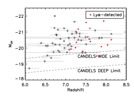
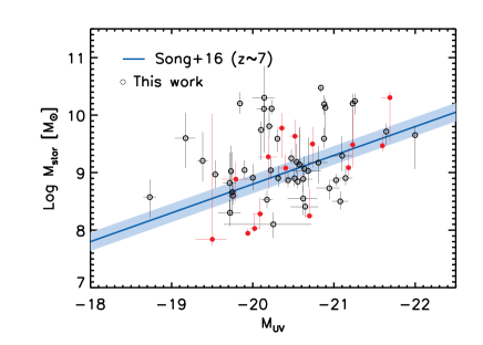
Figure 1: (Left) $M_{\text{UV}}$ distribution of target galaxies in our MOSFIRE observations in the GOODS-N as a function of redshift. Open circles display observed targets with photometric redshifts, and Ly$\alpha$ emitters are denoted as filled red circles with spectroscopic redshifts (Ly$\alpha$ emitters are further discussed in Section 3). The gray curves denote the limiting $M_{\text{UV}}$ in terms of the CANDELS/HST $J_{125}$ imaging depths: dashed and dotted-dashed lines are derived from the GOODS-N Deep and GOODS-N Wide fields, respectively. The reason why we have no Ly$\alpha$ detection at $z<7$ is that the transmission curve of the MOSFIRE $Y$-band filter drops at $\sim$9800Å (corresponding to Ly$\alpha$ at $z\sim 7$). (Right) $M_{\text{star}}$ – $M_{\text{UV}}$ relation of the target galaxies. The blue solid line shows the fiducial $z\sim 7$ relation of Song et al. (2016b) with the shaded area of its uncertainty. Our spectroscopic sample is drawn fairly uniformly from this trend, showing no significant sample bias relative to the underlying galaxy population.

2 Data

2.1 Texas Spectroscopic Search for Ly$\alpha$ Emission at the End of Reionization

Our spectroscopic data were obtained through a total of 18 nights of spectroscopic observations in the GOODS fields with Keck/DEIMOS (PI: R. Livermore, published in Jung et al., 2018) and Keck/MOSFIRE (the majority awarded through the NASA/Keck allocation; PI: S. Finkelstein). The GOODS-S MOSFIRE observations were published in Song et al. (2016a), and Jung et al. (2019) published the deepest ($>$16hr) MOSFIRE dataset in GOODS-N.

2.2 MOSFIRE $Y$-band Observations in GOODS-N

In this study, we analyze the entire MOSFIRE dataset in GOODS-N, targeting 72 $z\gtrsim 7$ galaxies over 10 nights of Keck/MOSFIRE observations with six mask designs from 2013 April to 2015 February. To cover Ly$\alpha$ over a redshift range of $z>7$, we used the $Y$-band filter which has a spectral resolution of $\sim 3$Å ($R=3500$). The slit width was chosen to be 0$\farcs$7 to match the typical seeing level at Maunakea. During our observations, individual frames were taken with 180 s exposures with an ABAB dither pattern (+1$\farcs$25, -1$\farcs$25, +1$\farcs$25, -1$\farcs$25). The details of the observations are described in Table 1 of Jung et al. (2019).

2.3 Physical Properties of Target Galaxies

Table 3 in the Appendix shows the list of the spectroscopic targets in our GOODS-N MOSFIRE observations. The target selection was based on the photometric redshift catalog of Finkelstein et al. (2013, 2015), utilizing the HST/CANDELS photometric catalog (Grogin et al., 2011; Koekemoer et al., 2011). Slitmask configurations were designed by MAGMA, maximizing the Ly$\alpha$ detection probability based on the galaxy brightness and the photometric redshift probability within the instrumental wavelength coverages. Although the MOSFIRE $Y$-band coverage for Ly$\alpha$ is limited at $z>7$, we include $z\gtrsim 6.5$ galaxies in the target selection, accounting for the photometric redshift uncertainties. At the time of target selection, the redshift information was based on the previous version of the photometric redshift catalog in Finkelstein et al. (2015). Recently, S. L. Finkelstein et al. (in preparation) has updated the photometric redshift measurements with updated CANDELS photometry including deep $I_{814}$ and Spitzer/IRAC data where they performed deblending of the low-resolution IRAC images with the HST images as priors. We use the updated photometric redshift catalog of S.L. Finkelstein et al. (in preparation) for our analysis, and 10 observed galaxies are now likely to be low-$z$ objects in the updated catalog and are excluded from the analysis for the remainder of this study.

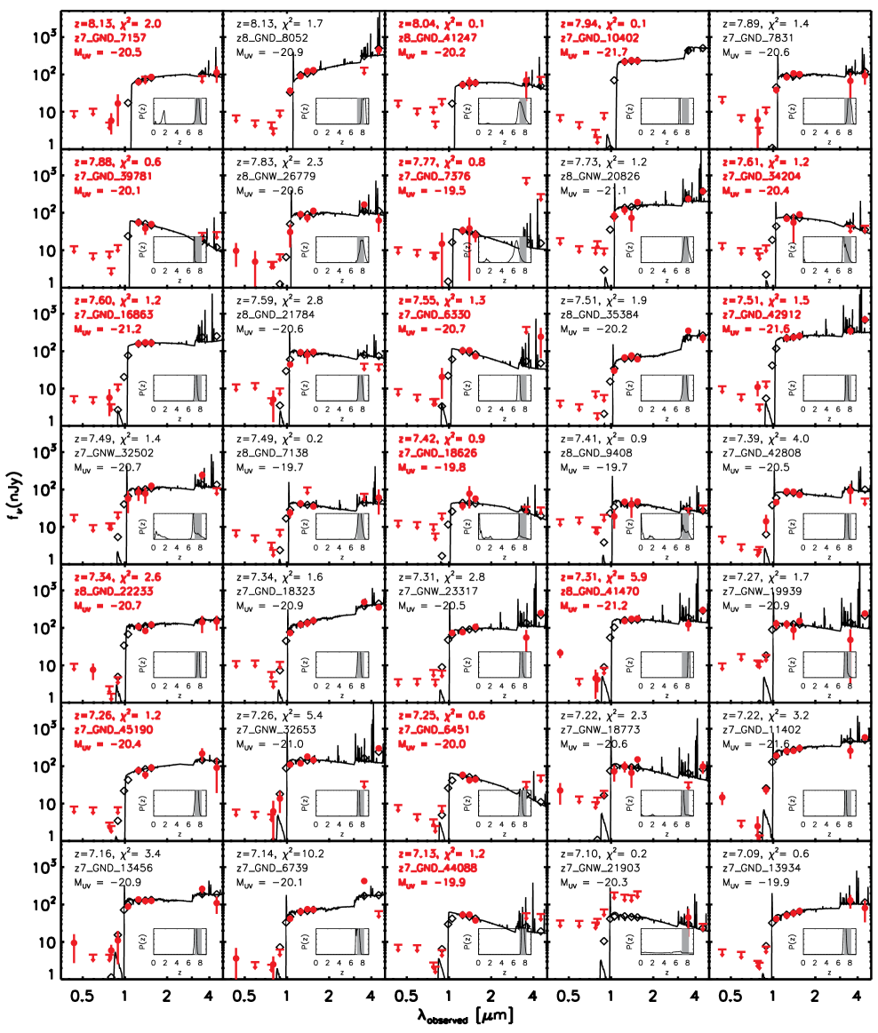
Figure 14: The best-fit models SEDs of $z>6$ galaxies among the entire sample. Each panel displays the best-fit model (solid curves and diamond symbols) with the observed photometry (red filled circles). Downward arrows denote 1$\sigma$ upper limits. The panels with red bold texts display Ly$\alpha$-detected galaxies. For Ly$\alpha$ non-detected galaxies, we assume galaxy redshifts as the peak redshift values of the photo-$z$ PDFs. The normalized photo-$z$ PDFs are shown in inset panels, and the shaded regions denote the instrumental redshift coverage of Ly$\alpha$ emission in MOSFIRE $Y$-band observations.

To understand the properties of our observed sources, we perform spectral energy distribution (SED) fitting with the Bruzual & Charlot (2003) stellar population model. We utilize HST/ACS ($B_{435}$, $V_{606}$, $i_{775}$, $I_{814}$ and $z_{850}$) and WFC3 ($Y_{105}$, $J_{125}$, $JH_{140}$ and $H_{160}$) broadband photometry and Spitzer/IRAC 3.6$\mu$m and 4.5$\mu$m band fluxes. We assume a Salpeter (1955) initial mass function with a stellar mass range of 0.1–100$M_{\odot}$, and a metallicity range of 0.005–1.0$Z_{\odot}$. We adopt a range of exponential models of star formation histories with various exponentially varying timescales ($\tau=$ 10 Myr, 100 Myr, 1 Gyr, 10 Gyr, 100 Gyr, -300Myr, -1 Gyr. -10 Gyr). We model galaxy spectra using the Calzetti (2001) dust attenuation curve with $E(B-V)$ values ranging from 0 to 0.8, and nebular emission lines are added as described in Salmon et al. (2015), which adopts the Inoue (2011) emission-line ratios. The intergalactic medium attenuation is considered based on Madau (1995). The best-fit models have been obtained minimizing $\chi^{2}$, and the uncertainties of physical parameters are estimated by performing SED fitting with 1000 Monte Carlo (MC) realizations of the perturbed photometric fluxes for individual galaxies. For the Ly$\alpha$-detected objects, we fit the model SEDs to the observed fluxes after subtracting the Ly$\alpha$ contributions in the continuum fluxes. UV magnitudes ($M_{\text{UV}}$) of galaxies are estimated from the averaged fluxes over a 1450–1550Å bandpass from the best-fit models. The best-fit model SEDs of our target galaxies are displayed in Figure 14 and 15 in the Appendix with the observed photometry.

The left panel in Figure 1 shows the $M_{\text{UV}}$ distribution of our GOODS-N MOSFIRE targets as a function of redshift. The black circles show the entire sample, and the red circles denote Ly$\alpha$-detected objects. As shown in the figure, our targets are randomly distributed over a wide range of $-19\lesssim M_{\text{UV}}\lesssim-22$ with fewer faint objects at increasing redshift. This is somewhat natural due to the limiting observational depths in the continuum observations at higher redshifts. The reason why we have no Ly$\alpha$ detection at $z<7$ is that the transmission curve of the MOSFIRE $Y$-band filter drops at $\sim$ 9800Å (corresponding to Ly$\alpha$ at $z\sim 7$). In the right panel, we display the $M_{\text{star}}$–$M_{\text{UV}}$ relation of our targets. Our galaxies are scattered out to broad regions in the relation, but consistent to the fiducial $z\sim 7$ measurement of Song et al. (2016b). Overall, our target selection does not exhibit a significant selection bias, representing the typical high-$z$ galaxy population at that redshift.

2.4 Data Reduction and Flux Calibration

We reduced the raw data using the most recent version of the public MOSFIRE data reduction pipeline (DRP). The DRP provides a sky-subtracted, flat-fielded, and rectified slit spectrum per object with a wavelength solution based on telluric sky emission lines. In the reduced two-dimensional (2D) spectra, the spectral dispersion is 1.09Å pixel^-1, and the spatial resolution is 0$\farcs$18 pixel^-1. However, a noticeable slit drift in the spatial direction has been reported in previous MOSFIRE observations (e.g., Kriek et al., 2015; Song et al., 2016a; Jung et al., 2019), and we also detected slit drifts of up to $\sim$pixel hr^-1. To correct for this slit drift, we reduced each adjacent pair of science frames separately, generating reduced 2D spectra for 360 s of integration time. We estimated the relative slit drift by tracing the positions of slit continuum sources (either stars or bright filler galaxies) in the spatial direction on the DRP-produced 2D spectra. Figure 2 shows the measured offsets in the spatial direction from the first frame as a function of time. Colors represent individual nights. The measured drifts are up to $\sim$ $0\farcs 1$ hr^-1. As this drift was a known issue at the time of our MOSFIRE observations, we aligned the telescope repeatedly in every 1–2 hr during some of the observations, shown as the breaking points in the plot.

The measured slit drift was corrected later when combining the individual DRP outputs. Running the DRP with a pair of frames makes it difficult to clean cosmic rays (CR) or bad pixels, thus we take sigma-clipped means in the combinations step in order to reject the bad pixels and CRs. To achieve an optimal signal-to-noise ratio (S/N), we weight the DRP outputs with the best-fit Gaussian peak fluxes of the continuum sources, which reflect observing conditions (e.g., seeing and transparency).

We performed long-slit observations of spectrophotometric standard stars for flux calibration and telluric absorption correction using Kurucz (1993) model stellar spectra. To obtain the response curve as a function of wavelength, we divided the model stellar spectra, which were scaled to match with the known photometric magnitudes of the standard stars, with the long-slit stellar spectra. We also corrected slit losses via flux calibration, considering the seeing condition of each night of observations.

As our science masks were observed in somewhat different observing conditions than the long-slit standard stars due to changing atmospheric conditions and airmass, we used continuum sources (stars) in our science masks to check for any residual flux calibration offset. We first applied the flux calibration from the spectrophotometric standard to our slitmask stars, then integrated these spectra through the HST/WFC3 $Y_{105}$ bandpass, and then compared these values to the $Y$-band magnitudes are taken from the updated photometric catalog of S. L. Finkelstein et al. (in preparation) based on the HST/CANDELS photometric data. We derived a residual normalization correction as the $Y$-band flux ratio between the known flux of these stars, and those derived from our MOSFIRE spectrum, such that after this correction was applied, they had the same $Y$-band magnitude. This residual normalization was up to $\sim$30-50%. As this correction can result in additional systematic errors in the flux calibration, it is recommended to have multiple continuum sources in science masks for future observations.

Each night of observations was calibrated individually, and some of the science masks were observed for multiple nights. We combined data from these masks after flux calibration, weighted with the best-fit Gaussian peak fluxes of the slit continuum sources. Also, we observed 49 galaxies in multiple masks; thus, these were combined with a weight factor based on the median-noise levels to generate a single fully reduced, all-mask-combined, and flux-calibrated 2D spectrum per object. The one-dimensional (1D) spectra of the sources were obtained via an optimal extraction (Horne, 1986) with a 1$\farcs$4 spatial aperture, twice the typical seeing level from our observations. For the optimal extraction, we built a spatial weight profile from the stellar profile so that the pixels near the peak of the stellar profile were maximally weighted.

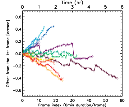
Figure 2: Offsets in the spatial direction from the first frame as a function of time, showing that objects drift in MOSFIRE slits along the spatial direction. This was corrected for during our data reduction, as described in Section 2.4. Different colors represent different nights of observations.

3 Results

3.1 Ly$\alpha$ Detections from an Automated Line Search

Although Ly$\alpha$ has been proven to be a useful method for confirming the redshifts of high-$z$ candidate galaxies, it becomes very challenging to detect into the epoch of reionization as it is sensitive to an increasing amount of neutral hydrogen in the IGM, and also becomes fainter as it is coming from more distant objects. Due to such hurdles, there have been only 10 Ly$\alpha$-emitting galaxies so far detected at $z>7.5$ (Finkelstein et al., 2013; Oesch et al., 2015; Zitrin et al., 2015; Song et al., 2016a; Laporte et al., 2017; Hoag et al., 2017; Hashimoto et al., 2018; Jung et al., 2019; Tilvi et al., 2020).

Another technical challenge of Ly$\alpha$ spectroscopic follow-up observations is in the search for faint emission-line features from obtained spectra, as it is difficult to distinguish them from noise peaks with human eyes. To perform a thorough scan on observed spectra, an automated approach has been adopted in previous studies (e.g., Jung et al., 2018; Larson et al., 2018; Pentericci et al., 2018a; Hoag et al., 2019), which can play a supplemental role to visual inspection, capturing missing plausible features.

In this work, we attempt to perform an improved automated search using the Source Extractor software (SExtractor; Bertin & Arnouts, 1996) on 2D spectra as well as Gaussian line fitting on 1D spectra (e.g., Larson et al., 2018). Figure 3 summarizes the entire procedure of our automated emission-line search. First we performed several iterations of visual inspection to search for any significant emission-line features, and estimated their detection levels as the S/N values of Ly$\alpha$ emission fluxes. To estimate emission-line properties, we performed asymmetric Gaussian fitting on reduced 1D spectra with the IDL MPFIT package (Markwardt, 2009). The asymmetric Gaussian function is defined as

$$f(\lambda)=f_{0}\times\begin{cases}\exp\Big{(}-\frac{1}{2}\frac{(\lambda-\lambda_{0})^{2}}{\sigma_{\text{blue}}^{2}}\Big{)}&\text{for}\ \lambda\leq\lambda_{0},\\ \exp\Big{(}-\frac{1}{2}\frac{(\lambda-\lambda_{0})^{2}}{\sigma_{\text{red}}^{2}}\Big{)}&\text{for}\ \lambda>\lambda_{0},\end{cases}$$ (1)

where $f_{0}$ is the peak value of the profile, $\lambda_{0}$ is the peak wavelength, $\sigma_{\text{blue}}$ and $\sigma_{\text{red}}$ are the blue- and red-side widths of the profile. In the fitting procedure, we have a zero continuum flux prior with initial guesses of $f_{0}=0.5\times 10^{-18}$ erg s^-1 cm^-2, $\lambda_{0}$ is at the peak flux wavelength in a 1D spectrum, and $\sigma_{\text{blue, red}}=3$Å. We adjust the wavelength range that is included in the fit for achieving the maximum S/N of the emission line by reducing nearby contaminations while still capturing the entire emission-line contribution. The associated errors of the physical quantities were derived from MC simulations by fluctuating the 1D spectra within their noise levels. From this visual inspection, we detect 13 emission-line features above a 3$\sigma$ level: 8 with S/N$>$4 and 5 with 3$<$S/N$<$4.

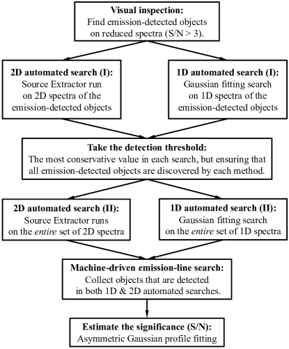
Figure 3: Graphical representation of our automated emission-line search procedures. The 1D automated search algorithm is adopted from Larson et al. (2018).

Then, to catch any emission features missed by the previous visual inspection, we applied the automated line search scheme of Larson et al. (2018) to the reduced 1D spectra and also ran Source Extractor on the reduced 2D flux and noise spectra. In the Source Extractor runs, we adjusted parameters to optimally search for point sources in 2D spectra with sizes comparable to the seeing value, typically $\sim$ 0$\farcs 7$ or 4 pixels in the spatial direction of the 2D spectra. In both 1D and 2D searches, we disregarded sky emission-line regions to avoid spurious emission features from sky residuals. However, the choice of a detection threshold in the automated searches is still arbitrary. A lower cut provides many more emission lines, which still include numerous false emission lines of, for example, uncleaned CRs, noise spikes, or contamination from nearby sources, while increasing the detection threshold would lose actual emission lines. Thus, we elected to place the highest detection thresholds where the automated searches still capture all of the 13 significant emission lines from our visual inspection, which is $\gtrsim$3$\sigma$ in the 1D search and $\gtrsim$4$\sigma$ in the Source Extractor runs.

With these detection thresholds, we examined the results of the 1D and 2D automated searches and found 29 emission features that were simultaneously detected by both 1D and 2D searches. This includes all previously detected emission lines from the visual inspection except for one tentative $\sim$3.5$\sigma$ detection from z8_GND_41470, as it was found very close to a sky emission line. Thus, applying the automated scans on 1D and 2D spectra found 17 additional plausible emission lines. Our improved automated search allows us to perform a machine-driven consistent emission-line search, where all plausible emission lines passed both automated searches with the same detection threshold as those from the visual inspection. Lastly, we measured S/N values for all plausible emission lines by performing asymmetric Gaussian fitting, which finds that 22 of these 29 lines have S/N$>$3; we discarded the 7 lower S/N sources. We visually inspected these 22 S/N $>$ 3 emission lines and found that five appeared to be sky residuals, and one appears spurious as it does not have the accompanying negative peaks expected for real sources due to our dithering sequence. Thus, our sample consists of 16 emission lines at $>$3$\sigma$ significance from this automated scanning, in addition to z8_GND_41470 (found visually). This automated search added three emission lines at a 4$\sigma$ level and one detection at a 3$\sigma$–4$\sigma$ level, which were not detected in visual inspection. This results in 17 significant emission lines: 11 with S/N$>$4 and 6 with 3$<$S/N$<$4.

Table 1: Summary of emission-line Properties

ID	$F_{\text{Ly}\alpha}$	S/N	EW${}_{\text{Ly}\alpha}$	$z_{\text{Ly}\alpha}$	$L_{\text{Ly}\alpha}$	H II Radii	$M_{\text{UV}}$	FWHM${}_{\text{red}}$	Log$(\sigma_{\text{red}}/\sigma_{\text{blue}})$	$\chi^{2}_{\text{Reduced}}$
	(10-17 erg s-1 cm-2)		(Å)		(1043 erg s-1)	(pMpc)		(km s-1)		$z_{\text{Ly$\alpha$}}(z_{\text{[{O\leavevmode\nobreak\ II}]}})$
(1)	(2)	(3)	(4)	(5)	(6)	(7)	(8)	(9)	(10)	(11)
z7_GND_44088	1.27$\pm$0.25	5.2	87.6${}^{+23.8}_{-21.2}$	7.1335$\pm$0.0028	0.79$\pm$0.16	0.88	-19.9	277${}^{+69}_{-91}$	0.77${}^{+3.37}_{-1.02}$	1.2 (7.2)
z8_GND_22233	1.36$\pm$0.19	7.1	54.5${}^{+15.0}_{-12.1}$	7.3444$\pm$0.0020	0.91$\pm$0.13	0.92	-20.7	264${}^{+75}_{-18}$	0.99${}^{+2.99}_{-0.89}$	2.6 (25.8)
z7_GND_18626	0.26$\pm$0.06	4.6	26.8${}^{+14.9}_{-9.8}$	7.4249$\pm$0.0013	0.18$\pm$0.04	0.52	-19.8	93${}^{+80}_{-71}$	3.54${}^{+0.97}_{-3.12}$	0.9 (2.8)
z7_GND_42912	1.46$\pm$0.13	10.8	33.2${}^{+4.3}_{-4.0}$	7.5056$\pm$0.0007	1.02$\pm$0.09	0.96	-21.6	266${}^{+57}_{-61}$	0.47${}^{+0.19}_{-0.21}$	1.5 (23.5)
z7_GND_6330	0.41$\pm$0.07	6.1	15.9${}^{+4.4}_{-3.7}$	7.5460$\pm$0.0006	0.29$\pm$0.05	0.62	-20.7	$<$88	0.43${}^{+2.33}_{-0.50}$	1.3 (16.9)
z7_GND_16863	1.89$\pm$0.18	10.8	61.3${}^{+14.4}_{-11.4}$	7.5989$\pm$0.0011	1.36$\pm$0.13	1.07	-21.2	411${}^{+6}_{-54}$	1.42${}^{+3.07}_{-0.80}$	1.2 (22.4)
z7_GND_34204	4.51$\pm$0.57	7.9	279.7${}^{+80.4}_{-62.5}$	7.6082$\pm$0.0030	3.26$\pm$0.41	1.44	-20.4	365${}^{+141}_{-88}$	0.27${}^{+0.60}_{-0.31}$	1.2 (5.2)
z7_GND_7376	0.26$\pm$0.06	4.1	32.5${}^{+23.0}_{-13.0}$	7.7681$\pm$0.0024	0.20$\pm$0.05	0.54	-19.5	147${}^{+69}_{-99}$	0.35${}^{+3.48}_{-0.89}$	0.8 (1.9)
z7_GND_39781	1.60$\pm$0.35	4.5	123.9${}^{+37.4}_{-32.9}$	7.8809$\pm$0.0018	1.25$\pm$0.27	1.04	-20.2	$<$85	-0.17${}^{+1.10}_{-3.25}$	0.6 (11.0)
z7_GND_10402	0.32$\pm$0.08	4.0	6.7${}^{+2.7}_{-2.2}$	7.9395$\pm$0.0023	0.26$\pm$0.06	0.59	-21.7	107${}^{+44}_{-92}$	0.94${}^{+5.40}_{-2.30}$	0.1 (97.0)
z7_GND_6451	0.68$\pm$0.21	3.2	43.2${}^{+17.2}_{-15.1}$	7.2462$\pm$0.0045	0.44$\pm$0.14	0.72	-20.0	93${}^{+65}_{-70}$	0.20${}^{+0.97}_{-1.22}$	0.6 (9.6)
z7_GND_45190	0.31$\pm$0.09	3.4	22.9${}^{+13.7}_{-9.3}$	7.2650$\pm$0.0019	0.20$\pm$0.06	0.55	-20.4	$<$91	-0.31${}^{+3.91}_{-2.75}$	1.2 (8.6)
z8_GND_41470	0.93$\pm$0.26	3.5	25.9${}^{+9.5}_{-8.4}$	7.3115$\pm$0.0028	0.61$\pm$0.17	0.81	-21.2	$<$90	-1.21${}^{+1.69}_{-3.54}$	5.9 (36.7)
z8_GND_41247	1.70$\pm$0.44	3.9	164.2${}^{+85.8}_{-60.5}$	8.0356$\pm$0.0015	1.39$\pm$0.36	1.07	-20.2	$<$83	-0.42${}^{+1.16}_{-3.36}$	0.1 (2.1)
z7_GND_7157	0.26$\pm$0.08	3.4	21.2${}^{+9.9}_{-8.0}$	8.1280$\pm$0.0016	0.22$\pm$0.07	0.56	-20.5	161${}^{+59}_{-127}$	1.28${}^{+3.70}_{-1.55}$	2.0 (3.4)

Note. — Col. (1) Object ID, (2) Ly$\alpha$ emission-line flux, (3) signal-to-noise ratio, (4) equivalent width of the Ly$\alpha$ emission line, (5) spectroscopic redshift based on the Ly$\alpha$ emission line, (6) Ly$\alpha$ emission luminosity, (7) radii of ionized H II bubbles around LAEs, based on the relation between Ly$\alpha$ luminosities and the bubble sizes from the Yajima et al. (2018) model (see more discussion in Section 5), (8) galaxy UV magnitude, estimated from the averaged flux over a 1450–1550Å bandpass from the best-fit galaxy SED model, (9) velocity FWHM, inferred from the red side of the emission line, corrected for the instrumental broadening, (10) asymmetry of the Ly$\alpha$ emission-line profile, where $\sigma_{\text{blue}}$ and $\sigma_{\text{red}}$ represent the blue- and red-side line widths, and (11) reduced $\chi^{2}$ values from the best-fit SED models of $z_{\text{Ly$\alpha$}}$ ($z_{\text{[{O\leavevmode\nobreak\ II}]}}$).

^aFive emission lines with S/N$<$4, listed at the bottom, are not included in the remainder of our analysis in Section 4 and 5.

^bListed uncertainties account for the UV-continuum measurement errors from SED fitting.

^cIn case that the measured values are smaller than the instrumental broadening, we provide the instrumental broadening as an upper limit.

^dKnown as z8_GND_5296 in Finkelstein et al. (2013) and updated in Jung et al. (2019). The source was observed in Tilvi et al. (2016) and Hutchison et al. (2019) as well.

^eLy$\alpha$ emission reported in Jung et al. (2019).

^fKeck/DEIMOS observations of Jung et al. (2018) displayed an emission-line feature at $z_{\text{Ly$\alpha$}}=6.70$, but it turned out to be contaminating O III emission from a nearby $z=0.87$ object (noted by Lennox Cowie).

3.2 Low-$z$ Interpretations

To further explore whether these lines are indeed Ly$\alpha$, we checked the possibility of other, lower-redshift, solutions. First, we checked multiple-emission-line objects with the other emission lines (e.g., [O III] $\lambda\lambda$4959, 5007, H$\beta$, [N II] $\lambda\lambda$6548, 6584, H$\alpha$) as the MOSFIRE spectral coverage would allow us to detect multiple lines in these low-$z$ objects. However, none of our objects show multiple emission lines from our emission-line search, which rules out their possibilities of being those emission lines listed except for either Ly$\alpha$ or [O II] $\lambda\lambda$3727, 3729.

Specifically, the strong continuum break with an emission line between the optical and NIR photometric bands indicates that the emission is either Ly$\alpha$ with the Lyman break or [O II] $\lambda\lambda$3727, 3729 with the Balmer break. In the case of the [O II] doublet, a peak separation of the doublet based on the wavelength in vacuum is 2.783Å from the atomic line List (from www.pa.uky.edu), and it would be $\sim$7 – 8Å at $z\sim 1.6$–$2.0$. Given the spectral resolution of Keck/MOSFIRE ($R=3500$ or $\sim$3Å), the doublet should be resolved if the emission line was indeed [O II]. Although no object displays the doublet emission lines, it is still possible that these might be [O II] emission. Due to many sky emission lines in the NIR and the somewhat low S/Ns of the detected lines, only one of the doublet could be detected while the other peak is either too faint to be detected or located in sky emission regions. Therefore, we performed SED fitting for all emission-line-detected galaxies using broadband photometry, fixing the redshift to both the high-$z$ (Ly$\alpha$) and low-$z$ ([O II]) solutions. We compared $\chi^{2}_{\text{reduced}}$ values between the high- and low-$z$ emission-line solutions (listed in Table 1) and removed two galaxies (z7_GND_43678 and z7_GND_36688) that do not clearly prefer high-$z$ solutions, as they exhibit significant fluxes in HST photometric bands which are blueward of the emission-line wavelength, which is not expected were the line Ly$\alpha$. Specifically, z7_GND_43678 displays a very poor SED fit ($\chi^{2}_{\text{reduced}}>$10) for the high-$z$ case, and its $z_{\text{Ly$\alpha$}}=7.69$ is greatly mismatched to its tightly constrained $z_{\text{phot}}=6.40^{+0.08}_{-0.09}$ (based on the detections in $I_{814}$ and $z_{850}$). We find similar results for z7_GND_36688 ($\chi^{2}_{\text{reduced}}>$5 for the high-$z$ solution). Additionally, the emission line from z7_GND_36688 is relatively less certain to be a real emission line with its low S/N = 3.6 while that from z7_GND_43678 appears more convincing (S/N = 5.4).

We attempted to identify these emission lines among the possible low-$z$ interpretations. However, a robust identification is difficult as we detect neither a double peak indicating [O II] emission nor multiple emission lines (indicating, e.g., H$\alpha$ with [N II]) from these galaxies. Their SED fits are also poor at their [O II] and H$\alpha$ emission redshifts, additional perplexities that remain on these emission lines. Thus, while we cannot identify which emission lines these are, we do not include either source in our list of Ly$\alpha$-emitting galaxies. Finally, we have 15 objects which show Ly$\alpha$ emission ($>$3$\sigma$) after this low-$z$ check: 10 with S/N$>$4 and 5 with 3$<$S/N$<$4. The 1D and 2D spectra of our Ly$\alpha$ emitters are displayed in Figure 4 and 5.

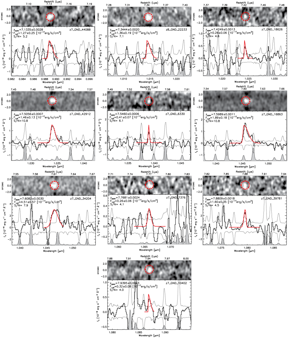
Figure 4: One- (bottom) and two-dimensional (top) spectra of our detected Ly$\alpha$ emission lines (S/N $>4\sigma$). In the 1D spectra, the black histogram is the all-mask-combined flux, smoothed by the instrumental resolution of $\sim 3$Å. The thin black curves represent the $1\sigma$ noise level, and the normalized sky emission is plotted at the bottom as a gray filled curve. Red curves show the best-fit asymmetric Gaussian curves. The displayed 2D spectra are the S/N maps that were obtained by dividing the sky-subtracted spectra by the noise spectra. The 2D spectra are smoothed by the instrumental resolution (x direction) and the seeing of the observations (y direction), and the dotted red circles denote detected emission lines.

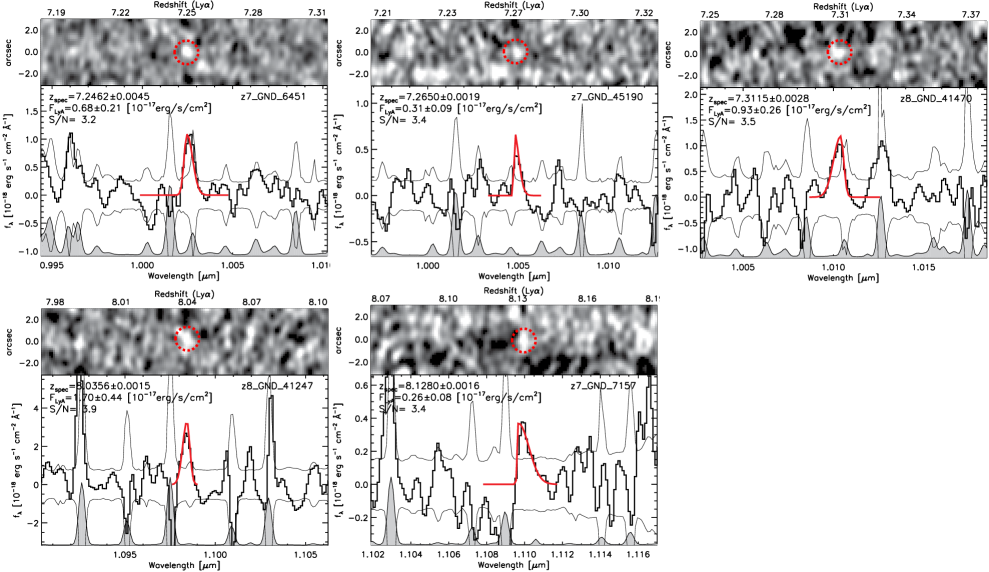
Figure 5: Same as Figure 4 but with S/N = 3$\sigma$–4$\sigma$.

3.3 False Detection Check in Automated Line Search

With the true spectra, our automated search provided 13 emission lines at S/N$>$4, and 11 of them were found to be actual emission lines with only one spurious source without negative counterparts and one another sky residual. To further explore the rate of spurious contamination in our emission-line selection process, we performed our automated search with the same detection criteria on negative versions of the 1D and 2D spectra. Across the negative versions of our observed galaxy spectra, we found eight S/N$>$4 emission lines. However, only one appears to represent a truly spurious detection. Two are sky residuals, and the other five are negative peaks caused by nearby contaminating objects, all of which would be flagged in our visual inspection on the true galaxy spectra. Thus, we conclude that our automated line search successfully delivers real emission lines with minimal spurious detection, although we still perform supplemental cleaning of sky residuals and spurious sources by visual inspection.

In addition, our 10 S/N$>$4 Ly$\alpha$ emission lines in Table 1 and Figure 4 are not likely spurious but securely detected Ly$\alpha$ as their 2D spectra display negative peaks on the top and the bottom sides, which emerge from the dithering pattern of the observations and would not be present for a spurious signal. We classify the five emission lines below 4$\sigma$ as tentative, needing further verification with deeper observations, and we do not include them in the remainder of our analysis for constraining the Ly$\alpha$ EW distribution. It is worth mentioning that if we perform the same analysis with all 15 emission lines, it does not significantly change our results and major conclusions.

3.4 Ly$\alpha$ Emission Properties

We derive the physical quantities of the detected emission lines by performing asymmetric Gaussian fitting on reduced 1D spectra, as described in the previous section. The derived line properties are summarized in Table 1.

Figure 6: Rest-frame EWs of Ly$\alpha$ emission lines vs. redshift (left) and $M_{\text{UV}}$ (right). Filled circles are S/N $>$ 4 LAEs, and the empty circles are 3 $<$ S/N $<$ 4 LAEs. We have 6 large-EW ($>$50Å) LAEs, which includes a $z=8.04$ LAE detected with S/N $=3.9$. Their $M_{\text{UV}}$ values span down to $-21.2$; thus, it appears that such large-EW LAEs are not limited to UV-faint objects. Interestingly, we detect one LAE with the extremely large EW of 280Å at $z=7.61$ without other AGN signatures (e.g., N V emission), which might require a very young and massive metal-poor stars.

3.4.1 Spectroscopic Confirmation of Galaxies at $z>7$

Our highest redshift Ly$\alpha$ emission line with S/N$>$4 is detected at $z_{\text{spec}}=7.94$ (z7_GND_10402). Overall, we detected 10 significant Ly$\alpha$ emission lines above a 4$\sigma$ level at $z>7$, discovering 5 new Ly$\alpha$ emission lines at $z>7.5$ with 2 previously known Ly$\alpha$ emitters at $z_{\text{spec}}=7.51$ and $7.60$ (Finkelstein et al., 2013; Jung et al., 2019). This increases the current number of confirmed Ly$\alpha$ emitters at $z>7.5$ from 10 to 15. Specifically, the spectroscopic confirmation rate at a $4\sigma$ level is $\sim$16% (10 Ly$\alpha$-confirmed over 62 $z_{\text{phot}}>6$ targets), which is achieved with $\sim$8hr of deep integration time per target on average. Although a spectroscopic confirmation rate strongly depends on target selection (photometric redshift PDFs and $M_{UV}$ distribution) in addition to the Ly$\alpha$ transmission in the IGM, this suggests that deep integrations make Ly$\alpha$ detections possible for many objects even out to $z\sim$ 8.

3.4.2 Large-EW Ly$\alpha$ Emission Lines

We derive the rest-frame EWs of the detected Ly$\alpha$ lines, listed in Table 1. The UV-continuum flux density for calculating EWs is the averaged flux density over a 1230–1280Å window of the best-fit SED model. Figure 6 shows the EWs vs. redshift (left) and $M_{\text{UV}}$ (right). As presented in Table 1 and Figure 6, we have six LAEs with EW $>$ 50Å  which includes a $z=8.04$ LAE detected with S/N $=$ 3.9 (also including the $z=7.6$ LAE in Jung et al., 2019), while previous measurements reported a deficit of these high-EW ($>$50Å) LAEs at $z>7$ (e.g., Tilvi et al., 2014). Along with the recent studies that find large-EW LAEs at $z\sim 7.5$ (Larson et al., 2018; Jung et al., 2019), our discovery of five additional large EW LAEs implies that such large-EW LAEs are less rare at this redshift than previously expected. Furthermore, their $M_{\text{UV}}$ values span down to $-21.2$; thus, it appears that such large-EW($>$50Å) LAEs are not limited to UV-faint objects, although no EW $\gtrsim 100$Å LAE is detected from UV-brighter ($M_{\text{UV}}<-20.5$) galaxies. To investigate further, we require a statistical number of LAEs.

Interestingly, z7_GND_34204 is emitting Ly$\alpha$ with EW = 280Å comparable to the typical theoretical limit ($\sim$ 240 – 350Å) of Ly$\alpha$ emission from star formation (Schaerer, 2003). Although it has been suggested that Ly$\alpha$ fluorescence illuminated by a nearby quasar could contribute to large-EW Ly$\alpha$ (Cantalupo et al., 2012; Rosdahl & Blaizot, 2012; Yajima et al., 2012), we did not detect an indicator of active galactic nucleus (AGN) activity from z7_GND_34204, for instance, a significant N V emission. Also, z7_GND_34204 has $M_{\text{UV}}=-20.4$, comparable but a little fainter than the characteristic population of $z\sim 7-8$ galaxies of $M_{\text{UV}}\sim-21$; thus, it seems that its large Ly$\alpha$ EW is less likely due to the AGN activity. Although it is challenging to interpret such extremely large-EW Ly$\alpha$ without AGN, Kashikawa et al. (2012) argue that their extremely large-EW Ly$\alpha$ emitter requires a very young and massive metal-poor stars like Population III stars (see also Schaerer, 2003; Raiter et al., 2010). Furthermore, Santos et al. (2020) reported a significant number of non-AGN LAEs with extreme EWs ($>$ 240Å) at $z\sim 2-6$. With all that being said, there seems to be an increasing demand for extreme stellar populations to explain these extremely large-EW LAEs.

3.4.3 Asymmetric Line Profile of Ly$\alpha$ Emission

Asymmetric line profiles are theoretically expected due to a combined effect of the ISM and IGM absorption, although complex Ly$\alpha$ radiative processes make it difficult to interpret the observed Ly$\alpha$ lines (e.g., Dijkstra, 2014). Within an optically thick medium, Ly$\alpha$ photons suffer resonant scattering with the H I gas, which redistributes the frequencies of the photons, shaping the line spectra into double-peaked profiles with an extremely opaque line center. In an outflowing medium, the emerging line profile has a stronger red peak than the blue peak due to the ISM kinematics, showing an asymmetric profile with sharp edges near the Ly$\alpha$ line center and extended red tails at their far sides (e.g., Verhamme et al., 2006). Specifically, the front side of the outflowing gas, which is moving toward us, has a relative velocity close to the resonance to the blueshifted Ly$\alpha$ photons (shorter wavelength photons) whereas the redshifted photons (longer wavelength photons) are less likely go through the resonance to the front side of the outflowing gas. Conversely, the red-side photons are likely scattered back toward us, being resonantly scattered by the back side of the outflowing gas, which is moving away from us (e.g., Dijkstra et al., 2014).

Recent studies of Green Pea galaxies, which are often referred to as local analogs of high-$z$ LAEs, have allowed detailed analyses including the internal kinematics to be constrained (e.g., Yang et al., 2016, 2017a, 2017b; Verhamme et al., 2018; Orlitová et al., 2018). At higher redshifts, asymmetric Ly$\alpha$ line profiles have been reported at $4<z<7$ (e.g., Rhoads et al., 2003; Dawson et al., 2007; Ouchi et al., 2010; Hu et al., 2010; Kashikawa et al., 2011; Mallery et al., 2012; U et al., 2015), though detailed physical modeling has not been possible.

In the high-$z$ universe, photons blueward of the Ly$\alpha$ line center are most likely absorbed by residual H I gas in the IGM. The resulting spectrum thus has only an asymmetric red peak observable. Additionally, into the epoch of reionization, the IGM absorption due to the damping wing optical depth could shape an asymmetric line profile with a sharp blue edge and an extended red tail (Weinberger et al., 2018). Along with this theoretical expectation, recent observational studies reveal this asymmetric shape of a Ly$\alpha$ emission line at $z>7$ from their deep spectroscopic observations (Oesch et al., 2015; Song et al., 2016a; Jung et al., 2019; Tilvi et al., 2020) while Pentericci et al. (2018a) report an asymmetric Ly$\alpha$ line profile from their stacked analysis of Ly$\alpha$ emission lines at $z\sim 7$. However, the occurrence of double-peaked Ly$\alpha$ emission has also been reported at these redshifts up to $z\gtrsim 6$ (Hu et al., 2016; Matthee et al., 2018; Songaila et al., 2018; Bosman et al., 2020). This suggests that a highly ionized and/or significantly inflowing medium could allow an escape of the blue-side Ly$\alpha$ photons.

Thanks to our deep spectroscopic observations along with Song et al. (2016a) and Jung et al. (2019), the analysis of the Ly$\alpha$ line profile is feasible for multiple sources. In Table 1, we present the measured asymmetry ($\sigma_{\text{red}}$/$\sigma_{\text{blue}}$) of the detected Ly$\alpha$ line profiles in the last column. Our measurements show asymmetric profiles of most Ly$\alpha$ emission lines with narrower blue-side profiles (Log$(\sigma_{\text{red}}$/$\sigma_{\text{blue}})>0$) in all S/N$>$4 Ly$\alpha$ emitters (except for z7_GND_39781), although only significant at the $\sim$1$\sigma$–2$\sigma$ level.

The FWHM values from the red side of the line profiles are listed in the second-to-last column, spanning from $\sim$90 – 410 km s^-1 with the median FWHM of $\sim$ $270$ km s^-1. Although the individual FWHM values largely vary, the median is comparable to those from the stacked spectra of LAEs at $z\sim 6-7$ from the previous studies: $270\pm 16$ and $265\pm 37$ km s^-1 at $z=5.7$ and $6.6$ from Ouchi et al. (2010), and $290\pm 25$ and $215\pm 20$ km s^-1 at $z\sim 6$ and $7$ from Pentericci et al. (2018a).

3.5 Photometric Redshift Calibration

The photometric selection technique of high-$z$ galaxies has brought an extensive set of candidate galaxies based on multiwavelength imaging data (e.g., Stark et al., 2009; Papovich et al., 2011; Bouwens et al., 2015; Finkelstein et al., 2015), and multiobject spectroscopic observations with photometrically selected galaxies have successfully confirmed their redshifts up to $z\gtrsim 8$ (e.g., Zitrin et al., 2015). Future observations with JWST/NIRSpec will be able to observe numerous fainter galaxies during the epoch of reionization with a much wider wavelength coverage of 0.9 – 5.0$\mu$m. This enables us to spectroscopically confirm their redshifts via a suite of rest-frame UV and optical lines as well as Ly$\alpha$ emission (Finkelstein et al., 2019a). However, photometric selection such as photometric redshift measurements (e.g., EAZY; Brammer et al., 2008) becomes more uncertain and needs to be calibrated further at $z\gtrsim 6$ (Pentericci et al., 2018a). Particularly, the so far rare spectroscopic confirmation of galaxies at $z>7.5$ makes it challenging to test photometric redshift measurement due to the faint nature of distant galaxies and the increasing neutral fraction of the IGM.

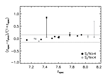
Figure 7: A comparison between spectroscopic redshifts and photometric redshifts. The Y-axis is the relative $\Delta z=(z_{\text{spec}}-z_{\text{phot}})/(1-z_{\text{spec}})$, and the dotted lines indicate thresholds for the catastrophic outlier of $\Delta z>0.15$ as defined in Dahlen et al. (2013) (see also Pentericci et al., 2018a). The overall quality of the photometric redshifts appears good, and all the relative errors of $\Delta z$ are less than the defined outlier thresholds within their uncertainties. However, there is a systematic bias seen at $z>7.4$ where the photometric redshifts are always underestimated compared to their spectroscopic redshifts.

Our comprehensive spectroscopic campaign now delivers new spectroscopic redshifts ($z_{\text{spec}}$) for 10 (15) galaxies at a 4$\sigma$ (3$\sigma$) level, including two previously known galaxies at $z=7.51$ and $7.60$ (Finkelstein et al., 2013; Jung et al., 2019). With these confirmed redshifts, we test the accuracy of our sample’s photometric redshifts ($z_{\text{phot}}$) as shown in Figure 7. We measure the relative error of $\Delta z=(z_{\text{spec}}-z_{\text{phot}})/(1-z_{\text{spec}})$ and define outliers at $|\Delta z|>0.15$ similarly to Dahlen et al. (2013). The overall quality of the photometric redshifts appears good, and all the relative errors of $\Delta z$ are less than the defined outlier thresholds within their uncertainties. However, there is a systematic bias at $z>7.4$ seen in the figure, where the photometric redshifts are always underestimated compared to the spectroscopic redshifts. A similar bias has been reported at various redshift ranges at $z>3$ in literature (e.g., Oyarzún et al., 2016; Brinchmann et al., 2017; Pentericci et al., 2018a). This is understandable in the sense that for Ly$\alpha$-detected objects, Ly$\alpha$ emission contributes to the increased flux at the photometric band which covers the observed wavelength range of Ly$\alpha$, and such increased flux pushes the continuum break (Lyman-break) toward shorter wavelengths in the photometric data.

Figure 8: The $3\sigma$ detection limit of an emission-line flux across the MOSFIRE instrument wavelength coverage, measured with 3Å spacing using a Monte Carlo simulation, inserting mock emission lines. We derive a linear relation between the line strength and its S/N level across the instrument wavelength coverage, and the detection limit of each simulated Ly$\alpha$ is interpolated from the precalculated linear relation. As the exposure time varies depending on each target, the detection limits are scaled by $\sqrt{t}$ to have 10hr of integration time for the purposes of this figure. The colored dots show the measured detection limit from the different galaxies, and the median detection limit is drawn as a black curve. Between the sky emission lines, the typical $3\sigma$ detection limit is as low as $\sim$ 2–3 $\times 10^{-18}$ erg s^-1 cm ^-2 for the targets observed in good observing conditions while 17 targets under poor observing conditions (2014 April, 2014 May, 2015 February) show three to four times higher detection limits.

4 Ly$\alpha$ Equivalent-width Distribution

4.1 Measuring the Ly$\alpha$ EW Distribution at $z\sim 7.6$

The Ly$\alpha$ EW distribution is often described by an exponential form, $P(\text{EW})\propto\text{exp}^{-\text{EW}/W_{0}}$, where $W_{0}$ is the $e$-folding scale (e.g., Cowie et al., 2010). As Treu et al. (2012, 2013) suggested, a Ly$\alpha$ study as a probe of reionization benefits from using the Ly$\alpha$ EW distribution (over the more traditional Ly$\alpha$ fraction) as it includes more information such as the Ly$\alpha$ flux and UV-continuum brightness, in addition to the detection rate (e.g., Tilvi et al., 2014; Mason et al., 2018a; Jung et al., 2018; Hoag et al., 2019). In Jung et al. (2018, J18 hereafter), we introduced a new methodology of measuring the Ly$\alpha$ EW distribution. We developed a simulation, which constructs a template of an expected number of Ly$\alpha$ emitters as a function of detection significance, by accounting for all types of data incompleteness, such as instrumental wavelength coverage, the wavelength-dependent Ly$\alpha$ detection limit, the UV-continuum flux, and the photometric redshift PDF. Here we apply this scheme to our MOSFIRE dataset to measure the Ly$\alpha$ EW distribution at $z>7$. As the MOSFIRE $Y$-band throughput allows us to detect Ly$\alpha$ at $7.0<z<8.2$, we limit the redshift range as $7.0<z<8.2$, placing our median constraint at $z\sim 7.6$.

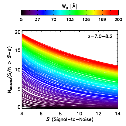
Figure 9: The expected number of emission lines as a function of S/N level ($\mathcal{S}$) with various EW distributions ($W_{0}=$5–200Å) at $z\sim 7.6$. A larger choice of the $e$-folding scale ($W_{0}$) of the Ly$\alpha$ EW distribution (redder color) predicts a larger number of detected Ly$\alpha$ emission lines.

To predict the expected number of Ly$\alpha$ emitters for a given EW distribution, we first need to calculate the detection sensitivity for each object’s spectrum. We precompute these via MC simulations with the 1D spectra by adding a mock Ly$\alpha$ emission line to the reduced 1D spectra for each object and recover the line flux of this mock line with its error in the same manner as we performed for the detected Ly$\alpha$ emission lines. We create this mock emission line having an intrinsic line profile equal to the best-fit asymmetric Gaussian profile of our highest-S/N Ly$\alpha$ emission detected in z7_GND_42912. This is a reasonable choice as the emission line from z7_GND_42912 has a somewhat representative shape of the line profile with its FWHM ($\sim$9Å) close to the median of all our S/N$>$4 emission lines. We estimate the Ly$\alpha$ detection sensitivity with 3Å spacing for all observed targets individually (Figure 8). This detection sensitivity reflects observing conditions, instrument throughput, and sky emission lines. As the shape of the mock emission-line profile could affect the estimated emission-line sensitivity, we test a narrower choice of the mock emission-line profile with FWHM = 5Å as well. Although its sharper profile provides a slightly lower detection limit, the overall difference of the line detection limit between FWHM = 5 and 9Å does not exceed the $\sim$10% level.

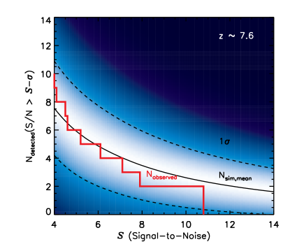
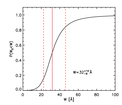
Figure 10: (Top) The probability distribution of the expected number of Ly$\alpha$ emission lines as a function of S/N level ($\mathcal{S}$) at $z\sim 7.6$, which is obtained from the $10^{5}$ MCMC chain steps. Higher probability regions are denoted by the brighter colors. The black solid curve shows the mean of the expected number of emission lines from our simulations as a function of S/N ($\mathcal{S}$), and the dashed curves are 1$\sigma$ uncertainties. Our 10 emission lines are drawn a red solid line. (Bottom) The cumulative probability of the EW $e$-folding scale ($W_{0}$) from our MCMC-based fitting algorithm at $z\sim 7.6$. The median value and 1$\sigma$ boundaries are denoted with solid and dashed red vertical lines, respectively.

With these sensitivities in hand, there are then three main steps to simulate the expected number of Ly$\alpha$ emitters in our dataset: (i) allocate the wavelength of the simulated Ly$\alpha$ emission, which is randomly drawn from an object’s photometric redshift PDF, (ii) estimate the line flux of the simulated Ly$\alpha$ by drawing an EW from the assumed Ly$\alpha$ EW distribution, $P(\text{EW})\propto\text{exp}^{-\text{EW}/W_{0}}$ given a value of $W_{0}$, multiplied by the UV-continuum flux of a galaxy, and (iii) calculate the S/N value of the simulation line using the precomputed wavelength-dependent Ly$\alpha$ detection limits. We follow these steps to calculate the expected number of detected emission lines as a function of line S/N for a given value of the $e$-folding scale $W_{0}$, in the range of $W_{0}$ = 5 – 200Å. For each choice of $W_{0}$, we perform 1000 sets of simulations, which produce a distribution of the expected number of Ly$\alpha$ emission lines as a function of S/N, shown in Figure 9. In this figure, each curve is the median average of 1000 MC runs for a corresponding $W_{0}$. With a larger choice of $W_{0}$, more Ly$\alpha$ emission lines detected at higher-S/N levels would be expected in observations.

Lastly, we fit our actual Ly$\alpha$ emission lines (10 emission lines with S/N$>$4) to these simulated distributions to calculate the PDF of the $e$-folding scale ($W_{0}$) of the Ly$\alpha$ EW distribution. Our fitting scheme is based on a Markov Chain Monte Carlo (MCMC) algorithm with a Poisson likelihood, as counting the number of Ly$\alpha$ emission lines is a general Poisson problem. We use the ”Cash statistic,” which describes the Poisson likelihood (Cash, 1979). Via the Metropolis-Hastings MCMC sampling (Metropolis et al., 1953; Hastings, 1970), we construct the PDF of $W_{0}$, generating 10⁵ MCMC chains. A more detailed explanation of our fitting procedure is described in Section 4 in J18.

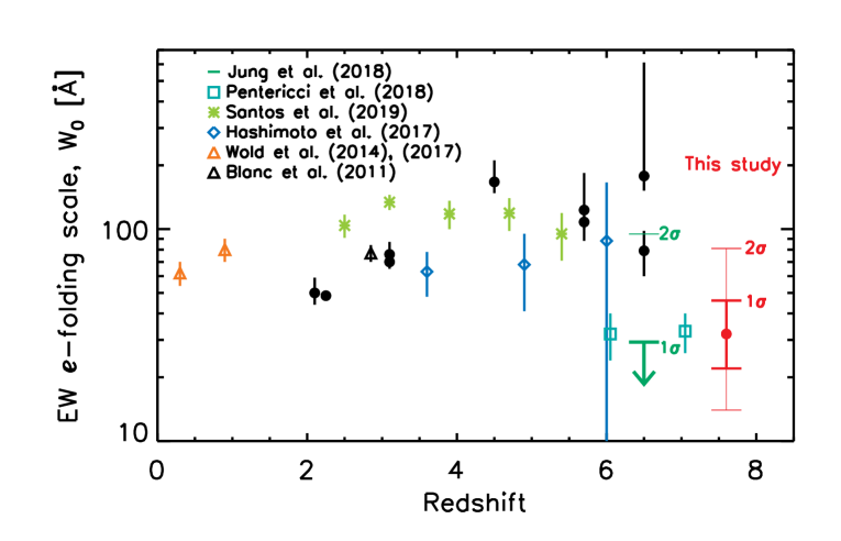
Figure 11: The redshift dependence of the Ly$\alpha$ EW $e$-folding scale ($W_{0}$) up to $z\sim 7.6$. All data are shown without an IGM absorption correction. Our $W_{0}$ measurements are denoted by a red filled circle at $7.0<z<8.2$. Our study provides a decreased $W_{0}$ of $32^{+14}_{-9}$Å at $z\sim 7.6$, whereas there is little/no redshift evolution of $W_{0}$ reported in the literature at $z<6$. Black filled circles are low-$z$ measurements drawn from a compilation of Zheng et al. (2014), including Guaita et al. (2010) at $z=2.1$, Nilsson et al. (2009) at $z=2.25$, Gronwall et al. (2007) at $z=3.1$, Ciardullo et al. (2012) at $z=3.1$, Ouchi et al. (2008) at $z=3.1,3.7$, Zheng et al. (2014) at $z=4.5$, Kashikawa et al. (2011) at $z=5.7$ and $6.5$, and Hu et al. (2010) at $z=5.7$ and $6.5$. Blue diamonds are the measurements of Hashimoto et al. (2017) at $z\sim 3$–6 using the LAEs ($M_{\text{UV}}<-18.5$) from the MUSE HUDF Survey (Bacon et al., 2017), which are consistent with Zheng et al. (2014) at that redshift range. At lower redshift, the $W_{0}$ measurements of Wold et al. (2017) at $z\sim 0.3$ and Wold et al. (2014) at $z\sim 0.9$ (orange triangles) suggest a relatively unevolving EW $e$-folding scale of Ly$\alpha$ across $z\sim 0.3-3.0$, considering the other measurements described above, including Blanc et al. (2011, black triangle) at $z\sim 2.85$. The green downward arrows at $z\sim 6.5$ are the measurements of Jung et al. (2018). Recent measurements from Pentericci et al. (2018a) and Santos et al. (2020) are shown as green squares at $z\sim 6$ and $7$ and yellowish-green asterisks at $2<z<6$. The $z\sim 6$ measurement from Pentericci et al. (2018a) is displayed at $z=6.1$ to avoid an overlap with the Hashimoto et al. (2017) data point. The measurements from J18, this work, and Pentericci et al. (2018a) at $z\gtrsim 6$ with the decreased values of $W_{0}$ are based on UV-continuum selection and show agreement within their uncertainties. However, there is some tension with other narrowband (NB) selection studies at the similar redshift (Hu et al., 2010; Kashikawa et al., 2011), and this is possibly due to sample selection biases between UV-continuum selection (J18, this study, and Pentericci et al., 2018a) and NB selection (the other studies in this figure).

Our MCMC sampling provides the PDF of $W_{0}$ at $7.0<z<8.2$, which is shown in the bottom panel of Figure 10. The median value of $W_{0}$ from the PDF is $32^{+14}_{-9}$Å (68% confidence level). The top panel of the figure presents a color-coded probability distribution of the expected number of Ly$\alpha$ emission lines at the corresponding S/N ($\mathcal{S}$) levels. The vertical axis shows the cumulative number of emission lines above $\mathcal{S}-\sigma$. The bright-shaded region shows the area of highest probability from our MCMC simulation, which matches the observed Ly$\alpha$ emission lines (red solid line).

4.2 Redshift Dependency of the Ly$\alpha$ EW $e$-folding Scale

J18 constrained the Ly$\alpha$ EW distribution, its characteristic $e$-folding scale ($W_{0}$), with a DEIMOS dataset at $z\sim 6.5$. A comparison of that to lower-redshift measurements in the literature suggests a suppressed Ly$\alpha$ visibility with a measured 1$\sigma$ (2$\sigma$) upper limit of $e$-folding scale at $<$36Å ($<$125Å), providing a weak sign of an increasing H I fraction in the IGM.

Here we add our data point at higher redshift, $7.0<z<8.2$, to our MOSFIRE observations, $W_{0}=32^{+14}_{-9}$Å, as shown in Figure 11. The figure displays a compilation of measurements in the literature at all redshifts, including our new measurement of $W_{0}$ at $z>7$, shown as the red filled circle at $z\sim 7.6$. Our result is lower than the $z<$ 6 observations ($W_{0}\sim$ 60–100Å) at 1$\sigma$ confidence. This is expected, particularly into the epoch of reionization, with a more opaque IGM. However, we cannot rule out no evolution at the 2$\sigma$ level.

Compared to the J18 measurement showing a rapid drop at $z>6$ in its 1$\sigma$ upper limit (the green downward arrow in Figure 11), our $z\sim 7.6$ measurement indicates a somewhat smoother decrease at $z>7$. This could be explained if reionization is inhomogeneous with regional variations in the IGM neutral fraction, though again these differences are not highly significant due to the somewhat large uncertainties.

J18 discuss some tension between their $z\sim 6.5$ measurement and other narrowband (NB) selection studies at the same redshift (Hu et al., 2010; Kashikawa et al., 2011), mentioning possible sample selection biases between UV-continuum selection (J18, this study, and Pentericci et al., 2018a) and NB selection (the other studies in Figure 11). Interestingly, the constrained $e$-folding scale values at $z\sim 6.5$ and $7.6$ from J18 and this study are mostly consistent with those at $z\sim 6$ and $7$ from Pentericci et al. (2018a). This agreement between continuum selection studies (and tension with the NB selection studies) might reflect possible biases caused by continuum selection where it misses large-EW LAEs from UV-faint galaxies. Such bias will be discussed in depth in the following section.

4.3 The $W_{0}$ Dependence on $M_{\text{UV}}$

The intrinsic shape of the Ly$\alpha$ EW distribution is known to be UV-magnitude dependent, and in general UV-bright galaxies have low EWs in Ly$\alpha$ (e.g., Ando et al., 2006; Stark et al., 2010; Schaerer et al., 2011; Cassata et al., 2015; Furusawa et al., 2016; Wold et al., 2017; Hashimoto et al., 2017; Jung et al., 2018). Additionally, Santos et al. (2020) present no significant redshift evolution of the Ly$\alpha$ EW at $W_{0}=129^{+11}_{-11}$ using the full sample of SC4K (Sobral et al., 2018) LAEs at $z\sim 2$ – 6, but find a strong $W_{0}$ dependency on $M_{\text{UV}}$ and stellar mass. Thus, we need to be careful to interpret the redshift dependence of the EW distribution, as sample selection of spectroscopic observations would place a bias on the derived $W_{0}$. Our MOSFIRE observations mostly targeted galaxies $M_{\text{UV}}\lesssim-19.5$ at $z>7$, missing significant UV-faint populations. This could impact on our derived $W_{0}$, biasing it toward a smaller value (e.g., Oyarzún et al., 2017; Hashimoto et al., 2018).

With the $M_{\text{UV}}$ dependency in mind, it is critical to perform a fair comparison of $W_{0}$ at the same $M_{\text{UV}}$ between different redshifts. We measure $W_{0}$ from different magnitude ranges and compare them to the lower-redshift values from Santos et al. (2020), which are summarized in Table 2. At all $M_{\text{UV}}$ ranges, we find that $W_{0}$ is significantly lower at $z\sim 7.6$, although in the brightest bin ($-22<M_{\text{UV}}<-21$), its $1\sigma$ upper limit overlaps with the lower-redshift value.

Importantly, recent studies have been reported a sign of different evolution of the Ly$\alpha$ EW in bright and faint objects into the epoch of reionization (e.g., Zheng et al., 2017; Mason et al., 2018b) whereas a decreasing $W_{0}$ with increasing UV-continuum brightness is seen at lower redshift (e.g., Ando et al., 2006; Stark et al., 2010; Schaerer et al., 2011; Cassata et al., 2015; Furusawa et al., 2016; Wold et al., 2017; Hashimoto et al., 2017; Oyarzún et al., 2017; Santos et al., 2020). Our measurements in Table 2 also show an apparent upturn of $W_{0}$ at the brightest magnitude bin, which is consistent with the other studies at this redshift. However, as the errors are large on these measurements, the result is also consistent with no upturn at the 1$\sigma$ level.

Table 2: Ly$\alpha$ EW $e$-folding scale ($W_{0}$) at Different $M_{\text{UV}}$

$M_{\text{UV}}$	Santos et al. (2020)	This Study
	$z\sim 2-6$	$z\sim 7.6$
$-20<M_{\text{UV}}<-19$	$178^{+13}_{-13}$Å	$61^{+64}_{-33}$Å
$-21<M_{\text{UV}}<-20$	$73^{+10}_{-10}$Å	$28^{+18}_{-9}$Å
$-22<M_{\text{UV}}<-21$	$54^{+11}_{-11}$Å	$48^{+63}_{-26}$Å
Full sample	$129^{+11}_{-11}$Å	$32^{+14}_{-9}$Å

4.4 Intrinsic Ly$\alpha$ Emitter Fraction

In our $W_{0}$ measurement, we simulate mock Ly$\alpha$ emission lines assuming all star-forming galaxies at this redshift are emitting Ly$\alpha$ as the galaxies are metal poor and contain less dust, which promotes the escape of Ly$\alpha$. However, it is not well known what fraction of LBGs at $z>7$ would be actually emitting Ly$\alpha$ if it were not absorbed by the IGM. Although the Ly$\alpha$ emitter fraction (LAF) increases with increasing redshift, it is below 50% at $z\lesssim 6$ (e.g., Stark et al., 2011; Curtis-Lake et al., 2012; Mallery et al., 2012). Thus, the assumption with an LAF of 100% may be too optimistic, even if the extrapolated LAF continuously increases at $z>6$.

Thus, we perform our $W_{0}$ measurement as described in Section 4.1 again, but assuming an intrinsic LAF of 50%. This gives a roughly doubled $W_{0}$ value of $67^{+54}_{-27}$Å from the entire sample: $83^{+71}_{-48},55^{+59}_{-26},$ and $100^{+65}_{-57}$Å at $-20$$<$$M_{\text{UV}}$$<$$-19$, $-21$$<$$M_{\text{UV}}$$<$$-20$, and $-22$$<$$M_{\text{UV}}$$<$$-21$, respectively. Although the measured $W_{0}$ values are still reduced at this redshift relative to the values at $z<7$, it is critical to understand the intrinsic LAF during the epoch of reionization in the future as it dramatically changes the inferred Ly$\alpha$ transmission in the IGM (see discussion in Section 5.1).

5 Constraints on Reionization

5.1 IGM H I Fraction Inference

5.1.1 Ly$\alpha$ Transmission in the IGM

A key quantity that we can draw from our measurement of the Ly$\alpha$ EW distribution is the Ly$\alpha$ transmission in the IGM, $T^{\text{Ly$\alpha$}}_{\text{IGM}}(=$EW${}_{\text{obs}}$/EW${}_{\text{int}})$, which compares the observed EW distribution (EW${}_{\text{obs}}$) to the intrinsic EW distribution (EW${}_{\text{int}}$). However, EW${}_{\text{int}}$ is not directly observable during the epoch of reionization as Ly$\alpha$ has likely been affected by H I in the IGM. Instead, to describe the intrinsic EWs at $z>6$, we utilize Ly$\alpha$ EWs obtained at $z<6$ (e.g., Santos et al., 2020) where we can assume that the universe is completely ionized. Although other measurements at $z\sim 6$ are available from De Barros et al. (2017) and Pentericci et al. (2018b), the reduced EWs from these studies suggest that reionization was not completed by $z\sim 6$, thus their EWs may be affected by residual H I in the IGM.

We assume no/little evolution of the interstellar medium (ISM) and circumgalactic medium (CGM) between $z<6$ and $z>6$ in this study, although a goal for future work is to figure out how the Ly$\alpha$ transmission in the ISM and CGM evolves over time in more detail (e.g., the evolution of the intrinsic Ly$\alpha$ escape fraction). Specifically, as shown in Figure 11, a compilation of Ly$\alpha$ EW measurements in the literature suggests no/little evolution of the $e$-folding scale ($W_{0}$) of the EW distribution at $\sim$100Å in the ionized universe at $z<6$ although the different sample selection methods and/or $M_{\text{UV}}$ dependency of $W_{0}$ make this difficult to interpret. With that in mind, this assumption allows us to separate the IGM attenuation from the ISM and CGM effect on the Ly$\alpha$.

It is critical to take the $M_{\text{UV}}$ dependency into account when estimating $T^{\text{Ly$\alpha$}}_{\text{IGM}}$ as the measured $W_{0}$ shows a clear $M_{\text{UV}}$ dependence. We thus utilize the $M_{\text{UV}}$-constrained $W_{0}$ values in Table 2 and estimate $T^{\text{Ly$\alpha$}}_{\text{IGM}}(=$EW${}_{z\sim\text{7.6}}$/EW${}_{z\sim\text{2--6}})=0.34^{+0.42}_{-0.19},0.38^{+0.35}_{-0.15}$, and $0.89^{+0.11}_{-0.55}$ at $-20<M_{\text{UV}}<-19$, $-21<M_{\text{UV}}<-20$, and $-22<M_{\text{UV}}<-21$, respectively. For the remainder of our analysis, we set $T^{\text{Ly$\alpha$}}_{\text{IGM}}$ = $0.38^{+0.35}_{-0.15}$ as our fiducial value, measured at $-21<M_{\text{UV}}<-20$ where the bulk of our spectroscopic sample lies (Figure 1).

5.1.2 Ly$\alpha$ Optical Depth in the IGM

From a theoretical perspective (e.g., Dijkstra, 2014; Mesinger et al., 2015; Mason et al., 2018a; Weinberger et al., 2018, 2019), $T^{\text{Ly$\alpha$}}_{\text{IGM}}$ is often described with an $e^{-\tau}$ modeling of the Ly$\alpha$ radiative transfer as

$$T^{\text{Ly$\alpha$}}_{\text{IGM}}=\frac{\int d\nu J(\nu)e^{-\tau_{\text{IGM}}(\nu)}}{\int d\nu J(\nu)},$$ (2)

where $J(\nu)$ is the intrinsic Ly$\alpha$ emission line from galaxies, and $\tau_{\text{IGM}}(\nu)$ is the IGM optical depth. The IGM optical depth, $\tau_{\text{IGM}}(\nu)$, is commonly considered as a combination of the damping wing optical depth due to diffuse H I during reionization ($\tau_{D}$) and the optical depth due to resonant scattering within the CGM of galaxies ($\tau_{\text{HII}}$) as $\tau_{\text{IGM}}(\nu)=\tau_{\text{D}}(\nu)+\tau_{\text{HII}}(\nu)$ (e.g., Dijkstra, 2014).

Although one can model the CGM contribution ($\tau_{\text{HII}}$) realistically with a combined description of reionization models (e.g., Weinberger et al., 2018), we take a simple approach by assuming no/little redshift variation of $\tau_{\text{HII}}$ at fixed $M_{\text{UV}}$ (or fixed halo mass) between $z<6$ and $z>6$.

5.1.3 H I Fraction in the IGM at $z\sim 7.6$

As an increasing neutral fraction ($X_{\text{HI}}$) in the IGM during the epoch of reionization determines the damping wing optical depth ($\tau_{D}$), the Ly$\alpha$ transmission in the IGM ($T^{\text{Ly$\alpha$}}_{\text{IGM}}$) is tied to $X_{\text{HI}}$, or the reionization history. A simplified analytical approach in Dijkstra (2014, their Equation 30) relates $X_{\text{HI}}$ with the damping wing optical depth as

$$\tau_{D}(z_{g},\Delta v)\approx 2.3X_{\text{HI}}\Big{(}\frac{\Delta v_{b}}{600\text{km s}^{-1}}\Big{)}^{-1}\Big{(}\frac{1+z_{g}}{10}\Big{)}^{3/2},$$ (3)

where $X_{\text{HI}}$ is the averaged neutral fraction of the IGM at a galaxy redshift $z_{g}$, and $\Delta v$ is the velocity offset of Ly$\alpha$ from the systemic redshift. $\Delta v_{b}$ represents a velocity offset from line resonance when a photon first enters a neutral cloud, written as $\Delta v_{b}=\Delta v+H(z_{g})R_{b}/(1+z_{g})$, where $H(z_{g})$ is the Hubble expansion rate, and $R_{b}$ is the comoving distance to the edge of the neutral cloud. Initially, $\tau_{D}$ is primarily dependent on frequency, characterized by the line profile and the velocity offset (also refer to Figure 5 in Mason et al., 2018a, for example). Thus, the frequency dependency is transformed to a $\Delta v$ dependency in the equation.

Once we relate the damping wing optical depth ($\tau_{D}$) to the estimated Ly$\alpha$ transmission of the IGM ($T^{\text{Ly$\alpha$}}_{\text{IGM}}$) following Equation (2), the primary uncertainties of the derived $X_{\text{HI}}$ in Equation (3) come from the velocity offset ($\Delta v$) and the distance of the first encounter to the closest neutral patch ($R_{b}$), which corresponds to the typical size of ionized bubbles at each redshift. Specifically, increasing $\Delta v$ and $R_{b}$ favors higher $X_{\text{HI}}$, which fosters an easier escape of Ly$\alpha$ photons before encountering a neutral IGM.

A typical observed range of the velocity offset at $z\gtrsim 6$ is $\sim$100 – 200 km s^-1 (Stark et al., 2015; Inoue et al., 2016; Pentericci et al., 2016; Mainali et al., 2017; Hutchison et al., 2019) while UV-luminous ($M_{\text{UV}}\lesssim-22$) systems reveal larger offsets (Willott et al., 2015; Stark et al., 2017). However, it is not feasible to directly measure $\Delta v$ from our observations without other metal lines detected. Instead, under the approximation that the FWHM of the Ly$\alpha$ emission equals the line velocity offset (Yang et al., 2017a; Verhamme et al., 2018), we infer the velocity offsets from the FWHM values of our S/N $>4$ detected Ly$\alpha$ emission lines of $\sim$ 90 – 410 km s^-1, using the mean value of $\sim$ 240 km s^-1 (Table 1).

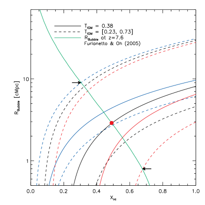
Figure 12: IGM neutral hydrogen fraction ($X_{\text{HI}}$) measurement. The plot displays the characteristic size of ionized bubbles ($R_{b}$) at $z=7.6$ as a function of $X_{\text{HI}}$ (green line) from Furlanetto & Oh (2005) as well as our $X_{\text{HI}}$ estimates as a function of $R_{b}$ (other lines) from the analytic approach of Dijkstra (2014). The bubble size ($R_{b}$) at $z=7.6$ is interpolated from the $z=6$ and $9$ values in Figure 1 of Furlanetto & Oh (2005). In our $X_{\text{HI}}$ calculation, each line represents a different combination of the Ly$\alpha$ transmission in the IGM ($T^{\text{Ly$\alpha$}}_{\text{IGM}}$) and the velocity offset ($\Delta v$). We explore $1\sigma$ upper and lower limits of $T^{\text{Ly$\alpha$}}_{\text{IGM}}$ = [0.23, 0.73] (dashed lines) as well as the median value of $T^{\text{Ly$\alpha$}}_{\text{IGM}}=0.38$ (solid lines), allowing a range of $\Delta v$ from 70 km s^-1 (blue) to 420 km s^-1 (red) with the fiducial value of 240 km s^-1 (black). The red dot indicates the estimated $X_{\text{HI}}\sim 49\%$ with the fiducial values of $T^{\text{Ly$\alpha$}}_{\text{IGM}}=0.38$ and $\Delta v=240$ km s^-1, simultaneously satisfying the predicted size of ionized bubble at a given $X_{\text{HI}}$ (corresponding to $R_{b}\sim 2.9$ cMpc) from the reionization model. The black arrows indicate $1\sigma$ limits of $X_{\text{HI}}$ at $\sim 30$ – $68\%$, conservatively allowing a range of $\Delta v=70$–$420$ km s^-1.

Although the damping wing optical depth ($\tau_{D}$) is strongly frequency dependent, dealing with the detailed modeling of the Ly$\alpha$ line profile is beyond the scope of this study. Instead, we assume no redshift evolution of the line profile in our analysis and adopt a representative value of the velocity offset from our observations. This is a reasonable approach under the assumption that ISM conditions are similar at the same $M_{\text{UV}}$, also shown in the observed empirical relation between $\Delta v-M_{\text{UV}}$ (e.g., Mason et al., 2018a).

As mentioned, the $X_{\text{HI}}$ calculation in Equation (3) is dependent on the characteristic size of ionized bubbles ($R_{b}$) as well, which can be predicted by reionization models (e.g., Furlanetto & Oh, 2005; Mesinger & Furlanetto, 2007). In Figure 12, the green line shows the characteristic bubble size at $z=7.6$ as a function of $X_{\text{HI}}$ based on the analytic model of reionization from Furlanetto & Oh (2005). The bubble size ($R_{b}$) at $z=7.6$ is interpolated from the $z=6$ and $9$ values in Figure 1 of Furlanetto & Oh (2005). The expected size of the bubbles in a highly ionized universe (low $X_{\text{HI}}$) would be larger than that in a more opaque universe (high $X_{\text{HI}}$). In Figure 12, we also plot our $X_{\text{HI}}$ estimates based on Equation (3) as a function of $R_{b}$. Each line represents a different combination of the Ly$\alpha$ transmission in the IGM ($T^{\text{Ly$\alpha$}}_{\text{IGM}}$) and the velocity offset ($\Delta v$): the median $T^{\text{Ly$\alpha$}}_{\text{IGM}}$ (solid) and its 1$\sigma$ limits (dashed), and $\Delta v=$ 70, 240, and 420 km s^-1 (blue, black, and red). The red dot indicates our fiducial value of $X_{\text{HI}}\sim 49\%$ with $T^{\text{Ly$\alpha$}}_{\text{IGM}}=0.38$ and $\Delta v=240$ km s^-1 (from the mean FWHM of the Ly$\alpha$ emission lines). This simultaneously satisfies the predicted size of the ionized bubble at a given $X_{\text{HI}}$ (corresponding to $R_{b}\sim 2.9$ cMpc) from the reionization model. In the figure, the black arrows indicate the $1\sigma$ limits of our $X_{\text{HI}}$ calculation at $\sim 30-68\%$, conservatively allowing a range of $\Delta v=70$–$420$ km s^-1.

The preferred size of the ionized bubbles, which satisfies the estimated $X_{\text{HI}}$, ranges from $\sim 1$–9 cMpc. Compared to a numerical model (Mesinger & Furlanetto, 2007), this analytic model of Furlanetto & Oh (2005) slightly underestimates the size of ionized bubbles as it does not take overlapping bubbles into account. However, the preferred bubble size here ($\sim 1$–9 cMpc) is still comparable to that predicted in Yajima et al. (2018) where they calculate the size of H II regions created by LAEs at $z\sim 8$ through semianalytic modeling: $\sim 2$–9 cMpc from $M_{\text{star}}=10^{8-10}M_{\odot}$ galaxies (see their Figure 10). Additionally, it is worth discussing the chance of detecting double-peaked Ly$\alpha$ emission from our LAEs as the recent discoveries of double-peaked Ly$\alpha$ emission at $z\gtrsim 6$ (Hu et al., 2016; Matthee et al., 2018; Songaila et al., 2018; Bosman et al., 2020) suggest that LAEs that reside in a highly ionized region could present double-peaked Ly$\alpha$ emission. Specifically, the preferred ionized bubble size from our calculation seems larger than the estimated bubble size of COLA1, a double-peaked LAE at $z=6.593$, which could form its $\sim$2.3 cMpc ionized bubble (Matthee et al., 2018). However, none of our LAEs at $z>7$ presents a significant sign of a double-peaked profile. This implies that the escape of blue-side photons of Ly$\alpha$ appears less feasible at $z>7$ possibly with an increasing IGM neutral fraction.

Although our $X_{\text{HI}}$ inference is inevitably sensitive to a reference value of the Ly$\alpha$ EW distribution at $z<6$ and reionization models, our inferred $X_{\text{HI}}\sim 49^{+19}_{-19}\%$ is lower in modest tension ($>$1$\sigma$) with results at similar redshifts: $X_{\text{HI}}=0.88$ at $z=7.6$, $>0.76$ at $z\sim 8$ (Hoag et al., 2019; Mason et al., 2019) and more comparable to the lower-redshift measurement of $X_{\text{HI}}=0.55$ at $z\sim 7$ (Mason et al., 2018a; Whitler et al., 2020). This could be due to the intrinsic inhomogenous nature of reionization. However, our result is consistent with what is predicted in Finkelstein et al. (2019b) of $X_{\text{HI}}$ $\sim$ $0.3^{+0.1}_{-0.1}$ at $z=7.6$, under the assumption that the faintest galaxies dominate the ionizing photon budget. It is also consistent with the neutral fraction of $X_{\text{HI}}=39^{+22}_{-13}\%$, which is estimated from the damping wing analysis of a luminous $z=7.5$ quasar observation in Yang et al. (2020). Additionally, as discussed in Section 4.4, the estimated $T^{\text{Ly$\alpha$}}_{\text{IGM}}$ would be doubled with a lower intrinsic LAF of 50%, making the corresponding $X_{\text{HI}}$ values even lower.

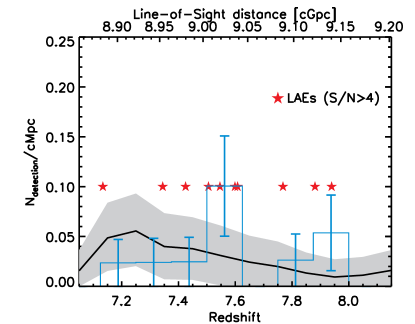
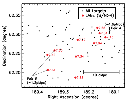
Figure 13: (Left) LAE overdensity at a function of redshift (or line-of-sight distance). The y-axis is the number of Ly$\alpha$ emission lines ($N_{\text{detection}}$) per unit volume, a 1 cMpc-thick slice in the line-of-sight (LOS) direction. The black curve is the expected number of emission lines based on our EW distribution modeling. The blue histogram shows actual Ly$\alpha$ emission lines, and its error bar is obtained with Poissonian statistics as $\sqrt{N_{\text{detection}}}$ in each bin. The red stars denote the individual spectroscopic redshifts of the detected LAEs. A notable feature is the peak near $z=7.5-7.6$ where we detect more LAEs than expected. Four LAEs at $z=7.51,7.55,7.60$, and $7.61$ are clustered within $\Delta z\sim 0.1$ (or 32.9 cMpc LOS distance). (Right) The spatial distribution of the detected LAEs (red circles) and all targets (black dots). The numbers next to red circles are the spectroscopic redshifts of the LAEs. The four clustered LAEs near $z=7.5-7.6$ are spread across the observed area, but still within 22.1 cMpc in the transverse direction. Particularly, two LAEs at $z=7.51$ and $7.55$ and the other two at $z=7.60$ and $7.61$ form close pairs, noted as “Pair A” and “Pair B” with their physical separations in parentheses in the plot. These clustered LAEs may indicate a sign of a large (with a $\sim$ 40 cMpc spatial extent) highly ionized structure (or multiple smaller ionized bubbles with the LAE pairs) in the early universe, showing directly the inhomogeneity of reionization.

5.2 Ionization Structure of the IGM

Reionization is an inhomogeneous process, starting in small ionized bubbles of the IGM around ionizing sources, the first stars and galaxies, with these bubbles expanding outward until the hydrogen in the IGM was completely ionized. The predicted size of these ionized bubbles thus becomes smaller with increasing redshifts (see the review of McQuinn, 2016).

Recent observations show growing evidence of ionized bubbles at $z>7$. Zheng et al. (2017) studied Ly$\alpha$ luminosity function (LF) from the Lyman Alpha Galaxies in the Epoch of Reionization Survey and reported a bump at the bright end of the Ly$\alpha$ LF at $z\sim 7$. They suggest that this is indicative of large ionized bubbles ($>$1 cMpc radius) and also different evolution between the bright and faint ends of the Ly$\alpha$ LF. Additionally, Castellano et al. (2018) presented a triplet of spectroscopically confirmed LAEs at the same redshift ($z=7.008$), which includes a pair of them at only $\sim$90 kpc distance. More recently, Tilvi et al. (2020) reported spectroscopic confirmation of three galaxies likely in a group (EGS77) at $z=7.7$ within $<0.7$ Mpc physical separation, forming up to $\sim$1 pMpc-size ionized bubbles.

Given our largest number of spectroscopically confirmed Ly$\alpha$ emitters from our survey, we explore spatial clustering of our detected LAEs at these high redshifts, and therefore, the inhomogeneity in the IGM. The left panel of Figure 13 presents a comparison between the number of detected LAEs (blue histogram) and the number of expected LAEs ($N_{\text{exp}}$: black solid line) from our survey as a function of redshift. The y-axis is $N_{\text{exp}}$ per 1 cMpc-thick slice in the line-of-sight (LOS) direction over the entire survey area, which is calculated as described in Section 4.1, assuming $W_{0}=32$Å. The shaded region represents the 1$\sigma$ uncertainty on $N_{\text{exp}}$, and the red stars denote the spectroscopic redshifts of the detected LAEs. A notable feature is the peak near $z=7.5$–$7.6$ where we detect more LAEs than expected, whereas we have Ly$\alpha$-detected objects which are less than/comparable to $N_{\text{exp}}$ in other redshift bins. Four LAEs at $z=7.51,7.55,7.60$, and $7.61$ are clustered within $\Delta z\sim 0.1$ (or 32.9 cMpc LOS distance). The right panel displays the 2D spatial distribution of our target galaxies (black dots) and the LAEs (red dots). The four clustered LAEs near $z=7.5-7.6$ are spread across the observed area, but still within 22.1 cMpc in the transverse direction (projection on the sky), and spread over a 3D spatial extent of 39.6 cMpc.

Particularly, z7_GND_42912 at $z=7.51$ and z7_GND_6330 at $z=7.55$ are in close proximity with each other with a 1.55 pMpc physical separation, marked as “Pair A” in the right panel of Figure 13. Along the LOS, the two galaxies are separated by 1.53 pMpc while in the transverse direction, they are separated by a mere 52$\farcs$7 (0.27 pMpc). Also, the other two galaxies (z7_GND_16863 and z7_GND_34204; “Pair B”) form a close pair at $z=7.60$ with a 1.15 pMpc physical separation. They are separated by only 0.35 pMpc along the LOS and by 3$\farcm$2 (0.95 pMpc) in the transverse direction.

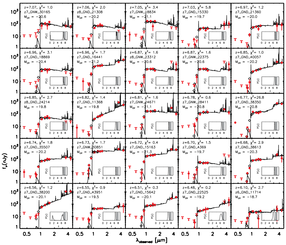
Figure 15: Continued from previous page.

Spectroscopic confirmation of $z>7$ galaxies via Ly$\alpha$ emission implies that these galaxies must be surrounded by ionized bubbles, making them visible in Ly$\alpha$ emission. Referring to the models from Yajima et al. (2018), and following Tilvi et al. (2020), the sizes of individual H II bubbles created by the galaxies could be roughly up to $\sim$1 pMpc. Specifically, z7_GND_42912 at $z=7.51$ (in Pair A) and z7_GND_16863 at $z=7.60$ (in Pair B) are massive ($M_{*}>10^{9}M_{\odot}$) and bright in their UV ($M_{\text{UV}}=-21.6$ and $-21.2$), which could be enough to form $\sim$1 pMpc-size ionized bubbles around them. As listed in Table 1, their Ly$\alpha$ luminosities are also bright ($>$10⁴³ erg s^-1) enough to form $\sim$1 pMpc-size ionized bubbles, based on the Yajima et al. (2018) model (see their Figure 15). Furthermore, z7_GND_34204 could form its largest $\sim$1.4 pMpc ionized bubble, suggested by its large EW ($=279.7$Å) and bright Ly$\alpha$ luminosity ($=3.26\times 10^{43}$ erg s^-1). Although our bubble size estimation is still model dependent, given their small separations in the two pairs ($\sim$1.6 pMpc in Pair A and $\sim$1.2 pMpc in Pair B), the individual H II bubbles in each pair likely overlap, forming a contiguous ionized region.

Relating to the H I fraction ($X_{\text{HI}}$) presented in the previous section, our lower $X_{\text{HI}}\sim 49\%$ is certainly driven by this potentially large ionized structure, and higher $X_{\text{HI}}$ values from other studies could be similarly driven by neutral regions. For instance, if we exclude the four clustered LAEs, the inferred $X_{\text{HI}}$ is increased to $58^{+23}_{-16}\%$ with $T^{\text{Ly$\alpha$}}_{\text{IGM}}$ = $0.22^{+0.21}_{-0.10}$ at $-21<M_{\text{UV}}<-20$, which is still lower than, yet more comparable to, other studies.

These clustered LAEs may indicate a sign of a large (with a $\sim$ 40 cMpc spatial extent) highly ionized structure (or multiple smaller ionized bubbles with the LAE pairs) in the early universe. Thus, our observations of the ionization structure provide an increasing body of evidence of inhomogeneous reionization caused by individual or a group of galaxies during the middle phase of the reionization epoch. Such inhomogeneities of reionization presented here demonstrate that future studies with much wider-field Ly$\alpha$ surveys will better constrain the global evolution of reionization.

6 Summary

We carried out our analysis on a comprehensive Ly$\alpha$ spectroscopic survey dataset with Keck/MOSFIRE at $z>7$, a subset of the Texas Spectroscopic Search for Ly$\alpha$ Emission at the End of Reionization survey (Jung et al., 2018, 2019). We reduced 10 nights of Keck/MOSFIRE observations, targeting 72 high-$z$ galaxies in the GOODS-N field with deep exposure times of $t_{\text{exp}}=4.5$ – 19 hr. Utilizing an improved automated emission-line search, we detect 10 Ly$\alpha$ emission lines at $z>7$ with $>$ 4$\sigma$ significance, and 5 more detections at a 3 – 4$\sigma$ level. By simulating the expected number of Ly$\alpha$ emission lines in our targets, we constrain the Ly$\alpha$ EW distribution at $7.0<z<8.2$ with the detected Ly$\alpha$ lines and infer the IGM H I fraction based on the Ly$\alpha$ transmission in the IGM. Also we study the spatial clustering of the LAEs to search for ionized structures during the epoch of reionization. Our major findings are summarized as follows.

1. We perform an automated search scheme on both 1D and 2D spectra to search in an unbiased way for plausible emission-line features, utilizing the automated 1D search algorithm of Larson et al. (2018) and the Source Extractor software (SExtractor; Bertin & Arnouts, 1996) on 2D spectra. Our automated search guarantees machine-driven consistency on detecting emission lines on 1D and 2D spectra, which supplement our visual inspection by discovering three more emission lines at the 4$\sigma$ level.

2. We detect 10 $z>7$ Ly$\alpha$ emission lines with S/N $>$ 4 and 7 at $z>7.5$, which includes our highest redshift Ly$\alpha$ emission with S/N $>$ 4 at $z_{\text{spec}}=7.94$. This significantly increases the total number of confirmed Ly$\alpha$ emission lines in this epoch.

3. Contradictory to the reported deficit of a high-EW ($>$50Å) LAE population at $z>7$ (e.g., Tilvi et al., 2014), we find six LAEs with EW$>$50Å, including one extremely large-EW (=280Å) LAE. Along with other recent studies of finding high-EW LAEs (Larson et al., 2018; Jung et al., 2019), our result supports that a high-EW population is not extremely rare in the high-$z$ universe.

4. We estimate the asymmetry of Ly$\alpha$ emission lines with $\sigma_{\text{red}}/\sigma_{\text{blue}}$ from asymmetric Gaussian fitting. Our result reveals that an asymmetric profile of Ly$\alpha$ emission is common in the early universe, although the modest S/N of our emission lines results in low-significance asymmetry for most sources.

5. With the largest number of spectroscopic confirmations of galaxies at $z>7$ in a single study, we test the accuracy of their photometric redshifts, measuring the relative error of $\Delta z$. We notice a systematic bias at $z>7.4$ where photometric redshifts are always underestimated compared to the spectroscopic redshifts, although the overall quality of $z_{\text{phot}}$ appears good.

6. We constrain the Ly$\alpha$ EW distribution at $7.0<z<8.2$, applying the methodology introduced in Jung et al. (2018), which constructs the PDF of the $e$-folding scale ($W_{0}$) of the EW distribution. Our constrained value of $W_{0}$ is $32^{+14}_{-9}$Å at $z\sim 7.6$, which is lower than lower-redshift values ($W_{0}\sim 100$Å). This implies an increasing H I fraction at this redshift, although the derived $W_{0}$ values considerably depend on assumptions made about the intrinsic fraction of Ly$\alpha$ emitters among galaxies at different redshifts.

7. We study the $W_{0}$ dependence on UV magnitude with our statistical sample. Contradictory to the expectation from low-$z$ studies, which show a decreasing $W_{0}$ with an increasing UV-continuum brightness, we find that there is an apparent upturn of $W_{0}$ at the brightest objects at $z\sim 7.6$, although the significance is low. This could be interpreted as a sign of different evolutions of Ly$\alpha$ EW between bright and faint objects during the epoch of reionization.

8. We infer the IGM H I fraction ($X_{\text{HI}}$) at $z\sim 7.6$ based on our estimated Ly$\alpha$ transmission ($T^{\text{Ly$\alpha$}}_{\text{IGM}}$) in the IGM. Adopting a simplified analytical approach, our estimated $T^{\text{Ly$\alpha$}}_{\text{IGM}}$ corresponds to $X_{\text{HI}}\sim 49^{+19}_{-19}\%$ at $z\sim 7.6$. This is lower than the other recent measurements of Ly$\alpha$ spectroscopic surveys (Hoag et al., 2019; Mason et al., 2019), but close to the predicted value of Finkelstein et al. (2019b), under the assumption that the ionizing photon budget from faint galaxies dominates.

9. A high Ly$\alpha$ detection rate at $z=7.5$ – $7.6$, where we detect four Ly$\alpha$ emission lines, indicates an overdense and highly ionized region. Particularly, two pairs of Ly$\alpha$ emitters at $z=7.51$ and $z=7.60$ likely form localized ionized bubbles. These clustered LAEs could be a sign of a large (with a $\sim$ 40 cMpc spatial extent) highly ionized structure (or multiple smaller ionized bubbles) in this early universe. The existence of such ionized structures in our survey area could explain our lower inferred value of $X_{\text{HI}}$, though due to the expected inhomogeneity of reionization, such structures may be a common feature in this epoch.

Recent measurements of the H I fraction from Ly$\alpha$ surveys reported an extremely high H I fraction ($X_{\text{HI}}$) at $z>7.5$: $X_{\text{HI}}$ = 0.88 at $z=7.6$, and $>$ 0.76 at $z\sim 8$ (Mason et al., 2019; Hoag et al., 2019). Although our estimation of $X_{\text{HI}}$ is based on a simplified analytic approach, our inferred $X_{\text{HI}}$ is below those high H I fractions from other Ly$\alpha$ studies. However, it is consistent with the recent measurement of $X_{\text{HI}}=39^{+22}_{-13}\%$ from the damping wing feature of a luminous $z=7.5$ quasar observations in Yang et al. (2020), showing that a lower $X_{\text{HI}}$ fraction is plausible at $z>$ 7.

To resolve such tension between recent measurements, a wide-field Ly$\alpha$ spectroscopic survey is necessary to grasp the entire picture of reionization, overcoming cosmic variance, particularly toward the end of reionization as reionization is inhomogeneous. Our spectroscopic survey proves that we are able to detect Ly$\alpha$ with deep exposures even into the epoch of reionization, while most previous Ly$\alpha$ observations at this redshift are relatively shallow, resulting in lower detection rates. Thus, a direct measurement of the Ly$\alpha$ EW distribution over a wider area with enough sensitivity to detect Ly$\alpha$ will be necessary to allow us to capture a more comprehensive picture of reionization.

Our results put observational constraints on the redshift dependence of the Ly$\alpha$ EW distribution during the epoch of reionization, particularly toward the end of reionization, accounting for all forms of data incompleteness. However, constraining the H I fraction in the IGM with Ly$\alpha$ is inevitably sensitive to reionization models (e.g., Mesinger et al., 2015; Kakiichi et al., 2016; Mason et al., 2018a; Weinberger et al., 2019). Thus, implementing a realistic calculation of Ly$\alpha$ radiative processes (e.g., Smith et al., 2019; Kimm et al., 2019) in future reionization models will place better predictions on how the expected Ly$\alpha$ EW distribution depends on the IGM neutral fraction. Moreover, the model predictions are dependent on many LAE systematics as well, such as the continuum luminosity, the interstellar medium (ISM) kinematics, and the stellar mass. For this purpose, a more comprehensive dataset covering various redshift ranges is required in order to investigate the Ly$\alpha$ systematics.

With the arrival of powerful future telescopes, this will be facilitated with great ease. In upcoming years, the James Webb Space Telescope (JWST) will be capable of exploring this in depth. The JWST/NIRSpec will have a wide NIR wavelength coverage, probing other UV metal lines, including C III], O II], and O III] lines for these high-$z$ galaxies. Utilizing other nonresonant metal lines allows us to derive the Ly$\alpha$ velocity offset with their systemic redshifts as shown in previous works (e.g., Erb et al., 2014; Steidel et al., 2016; Stark et al., 2017). Investigating Ly$\alpha$ velocity offsets at high redshifts and comparing the velocity offsets between high- and low-$z$ LAE populations will provide a better understanding of the Ly$\alpha$ systematics. On the ground, the extremely large telescopes, such as the Giant Magellan Telescope (GMT) and the Thirty Meter Telescope (TMT), will play critical roles in exploring the reionization topology. Although JWST will probe key physical quantities of high-$z$ galaxies, a much wider field coverage of the GMT is necessary to grasp the entire picture of reionization, overcoming cosmic variance and capturing the inhomogeneous nature of reionization. Plus, the TMT with its planned NIR instrument, IRMS, will probe even fainter objects, utilizing its larger collecting area (refer to Finkelstein et al., 2019a, for more discussion on Ly$\alpha$ studies with the extremely large telescopes).

Appendix A Summary of MOSFIRE Targets with Observed Spectral Energy Distributions

We display the best-fit model SEDs of $z>6$ galaxies among entire sample in Figures 14 and 15. All spectroscopic targets in our observations are list in Table 3.

Table 3: Summary of MOSFIRE Targets in GOODS-N

ID	R.A.	Decl.	$t_{\text{exp}}$	$J_{\text{125}}$	$M_{\text{UV}}$	$z_{\text{phot}}$	$z_{\text{spec}}$	EW${}_{\text{Ly}\alpha}$
	(J2000.0)	(J2000.0)	(hrs)					(Å)
z7_GND_7157	189.225125	62.286292	5.8	26.8	-20.5	7.54${}^{+0.21}_{-5.82}$	8.128 (3.4)	21.2${}^{+9.9}_{-8.0}$
z8_GND_8052	189.270000	62.288558	6.3	26.5	-20.9	8.13${}^{+0.27}_{-0.26}$	-	$<$42.1
z8_GND_41247	189.279500	62.179753	4.5	27.1	-20.2	7.29${}^{+0.46}_{-0.48}$	8.036 (3.9)	164.2${}^{+85.8}_{-60.5}$
z7_GND_10402	189.179292	62.275894	12.0	25.5	-21.7	6.59${}^{+0.06}_{-0.04}$	7.939 (4.0)	6.7${}^{+2.7}_{-2.2}$
z7_GND_7831	189.177292	62.291050	4.5	26.6	-20.6	7.89${}^{+0.27}_{-0.24}$	-	$<$32.6
z7_GND_39781	189.251708	62.185944	4.5	27.1	-20.1	6.94${}^{+0.02}_{-0.03}$	7.881 (4.5)	123.9${}^{+37.4}_{-32.9}$
z8_GNW_26779	189.286958	62.318019	5.5	26.5	-20.6	7.83${}^{+0.76}_{-0.32}$	-	$<$23.7
z7_GND_7376	189.243167	62.285039	5.8	27.6	-19.5	6.45${}^{+0.43}_{-0.77}$	7.768 (4.1)	32.5${}^{+23.0}_{-13.0}$
z8_GNW_20826	189.401167	62.319225	7.2	26.2	-21.1	7.73${}^{+0.39}_{-0.37}$	-	$<$66.4
z7_GND_34204	189.359708	62.205972	4.5	26.8	-20.4	7.08${}^{+0.35}_{-0.29}$	7.608 (7.9)	279.7${}^{+80.4}_{-62.5}$
z7_GND_16863	189.333083	62.257236	16.2	25.9	-21.2	7.21${}^{+0.13}_{-0.13}$	7.599 (10.8)	61.3${}^{+14.4}_{-11.4}$
z8_GND_21784	189.203125	62.242486	4.5	26.5	-20.6	7.59${}^{+0.24}_{-0.24}$	-	$<$30.8
z7_GND_6330	189.166250	62.316497	4.5	26.4	-20.7	6.87${}^{+0.14}_{-0.14}$	7.546 (6.1)	15.9${}^{+4.4}_{-3.7}$
z8_GND_35384	189.232000	62.202342	4.5	26.8	-20.2	7.51${}^{+0.25}_{-0.27}$	-	$<$190.4
z7_GND_42912	189.157875	62.302372	16.5	25.5	-21.6	7.43${}^{+0.11}_{-0.12}$	7.506 (10.8)	33.2${}^{+4.3}_{-4.0}$
z7_GNW_32502	189.285833	62.354964	7.2	26.6	-20.7	7.49${}^{+0.64}_{-6.49}$	-	$<$93.1
z8_GND_7138	189.121208	62.286400	5.8	27.3	-19.7	7.49${}^{+0.33}_{-0.33}$	-	$<$33.1
z7_GND_18626	189.360667	62.245567	5.5	27.5	-19.8	0.35${}^{+6.61}_{-0.30}$	7.425 (4.6)	26.8${}^{+14.9}_{-9.8}$
z8_GND_9408	189.300125	62.280358	19.0	27.2	-19.7	7.41${}^{+0.44}_{-7.18}$	-	$<$39.4
z7_GND_42808	189.188417	62.303050	4.5	26.5	-20.5	7.39${}^{+0.15}_{-0.15}$	-	$<$36.1
z8_GND_22233	189.249792	62.241225	6.3	26.3	-20.7	7.64${}^{+0.11}_{-0.12}$	7.344 (7.1)	54.5${}^{+15.0}_{-12.1}$
z7_GND_18323	189.371417	62.252139	10.0	26.2	-20.9	7.34${}^{+0.21}_{-0.19}$	-	$<$19.4
z7_GNW_23317	189.439667	62.302383	7.2	26.7	-20.5	7.31${}^{+0.15}_{-0.15}$	-	$<$109.4
z8_GND_41470	189.224458	62.311325	13.0	25.9	-21.2	8.19${}^{+0.08}_{-0.08}$	7.311 (3.5)	25.9${}^{+9.5}_{-8.4}$
z7_GNW_19939	189.273375	62.324783	12.7	26.2	-20.9	7.27${}^{+0.16}_{-0.17}$	-	$<$17.4
z7_GND_45190	189.138500	62.275600	10.2	26.7	-20.4	7.38${}^{+0.24}_{-0.23}$	7.265 (3.4)	22.9${}^{+13.7}_{-9.3}$
z7_GNW_32653	189.278750	62.357453	7.2	26.2	-21.0	7.26${}^{+0.10}_{-0.12}$	-	$<$61.7
z7_GND_6451	189.222000	62.315761	12.0	27.0	-20.0	7.24${}^{+0.14}_{-0.15}$	7.246 (3.2)	43.2${}^{+17.2}_{-15.1}$
z7_GNW_18773	189.309167	62.362142	7.2	26.4	-20.6	7.22${}^{+0.30}_{-0.22}$	-	$<$78.5
z7_GND_11402	189.186167	62.270864	12.0	25.4	-21.6	7.22${}^{+0.08}_{-0.08}$	-	$<$5.8
z7_GND_13456	189.264958	62.265789	11.8	26.1	-20.9	7.16${}^{+0.12}_{-0.12}$	-	$<$12.7
z7_GND_6739	189.260417	62.289403	5.8	26.9	-20.1	7.14${}^{+0.23}_{-0.29}$	-	$<$26.6
z7_GND_44088	189.135000	62.291869	10.7	27.1	-19.9	7.59${}^{+0.21}_{-0.20}$	7.133 (5.2)	87.6${}^{+23.8}_{-21.2}$
z7_GNW_21903	189.290750	62.311100	11.8	27.1	-20.3	7.10${}^{+5.26}_{-4.99}$	-	$<$27.8
z7_GND_13934	189.275917	62.260303	5.5	27.1	-19.9	7.09${}^{+0.16}_{-0.17}$	-	$<$41.4
z7_GNW_30165	189.327958	62.298572	5.5	26.3	-20.6	7.07${}^{+0.40}_{-6.44}$	-	$<$15.7
z8_GND_21308	189.109500	62.238792	5.8	26.8	-20.2	7.06${}^{+0.17}_{-0.12}$	-	$<$17.9
z7_GNW_18834	189.273292	62.360786	7.2	25.8	-21.1	7.05${}^{+0.21}_{-0.21}$	-	$<$46.3
z7_GND_15330	189.310875	62.260447	11.8	27.2	-19.7	7.03${}^{+0.14}_{-0.13}$	-	$<$36.4
z7_GND_21360	189.299458	62.236889	5.5	27.0	-20.0	6.97${}^{+0.11}_{-0.10}$	-	$<$31.7
z7_GND_18869	189.205292	62.250767	16.5	26.4	-20.4	6.96${}^{+0.02}_{-0.05}$	-	$<$11.9
z7_GND_16441	189.082667	62.252475	5.8	25.8	-21.2	6.96${}^{+0.12}_{-0.11}$	-	$<$8.2
z8_GNW_23312	189.166250	62.316497	6.3	26.4	-20.6	6.87${}^{+0.14}_{-0.14}$	-	$<$24.6
z7_GNW_22375	189.166250	62.316497	19.0	26.4	-20.6	6.87${}^{+0.14}_{-0.14}$	-	$<$17.9
z7_GND_40057	189.339458	62.184781	4.5	26.7	-20.2	6.85${}^{+0.17}_{-0.16}$	-	$<$136.3
z8_GND_24214	189.201042	62.227439	5.8	27.1	-19.8	6.85${}^{+0.07}_{-0.09}$	-	$<$26.2
z7_GND_11368	189.283708	62.272244	11.8	26.9	-19.8	6.82${}^{+0.18}_{-0.18}$	-	$<$48.1
z7_GNW_24671	189.361708	62.294372	7.2	25.9	-21.1	6.81${}^{+0.05}_{-0.07}$	-	$<$45.5
z7_GNW_28411	189.392708	62.308617	5.5	25.9	-20.8	6.78${}^{+0.11}_{-0.18}$	-	$<$15.0
z7_GND_38350	189.177167	62.291519	5.8	26.2	-20.8	6.77${}^{+0.06}_{-0.06}$	-	$<$16.3
z7_GND_35507	189.304458	62.201678	4.5	26.7	-20.2	6.74${}^{+0.07}_{-0.07}$	-	$<$122.0
z7_GNW_30851	189.356875	62.295319	5.5	24.7	-22.0	6.73${}^{+0.04}_{-0.04}$	-	$<$4.6
z7_GND_15163	189.079833	62.256458	5.8	25.6	-21.3	6.72${}^{+0.12}_{-0.11}$	-	$<$7.2
z7_GND_4369	189.187333	62.318822	5.8	27.3	-19.7	6.70${}^{+0.18}_{-0.17}$	-	$<$24.6
z7_GND_38613	189.155292	62.286461	5.8	26.6	-20.3	6.68${}^{+0.05}_{-0.05}$	-	$<$17.8
z7_GND_36688	189.178125	62.310639	5.8	27.4	-	6.64${}^{+0.23}_{-0.23}$	-	-
z7_GND_38200	189.359167	62.192122	4.5	26.6	-20.1	6.56${}^{+0.28}_{-5.08}$	-	$<$157.6
z7_GND_43951	189.154625	62.292919	12.0	27.3	-19.5	6.55${}^{+0.11}_{-0.11}$	-	$<$30.1
z7_GND_15642	189.151958	62.259639	12.0	26.8	-20.1	6.51${}^{+0.21}_{-0.20}$	-	$<$21.2
z7_GND_22525	189.372833	62.240372	10.0	27.6	-19.2	6.48${}^{+0.47}_{-0.53}$	-	$<$73.1
z7_GND_43678	189.235208	62.295594	6.3	26.5	-	6.40${}^{+0.08}_{-0.09}$	-	-
z6_GND_11714	189.323917	62.271114	6.3	28.2	-18.7	6.10${}^{+0.25}_{-0.27}$	-	$<$105.1
z6_GNW_20715	189.339875	62.319981	7.2	25.9	-	5.54${}^{+0.07}_{-0.07}$	-	-
z7_GND_22483	189.146417	62.240519	16.5	26.9	-	4.51${}^{+0.16}_{-0.26}$	-	-
z6_GND_12175	189.172042	62.269725	6.3	28.2	-	1.88${}^{+1.15}_{-1.39}$	-	-
z7_GND_22782	189.353000	62.232217	5.5	25.2	-	1.55${}^{+0.08}_{-0.08}$	-	-
z7_GND_25452	189.136583	62.223317	5.8	25.2	-	1.53${}^{+0.05}_{-0.05}$	-	-
z8_GND_7253	189.264250	62.285675	5.5	27.1	-	1.30${}^{+0.29}_{-0.10}$	-	-
z6_GND_41772	189.161083	62.309928	6.3	27.2	-	1.14${}^{+4.38}_{-0.15}$	-	-
z6_GND_39946	189.319583	62.185250	4.5	26.7	-	1.02${}^{+4.53}_{-0.24}$	-	-
z8_GNW_20236	189.433500	62.322303	7.2	26.1	-	0.69${}^{+6.09}_{-0.02}$	-	-
z7_GND_11273	189.100375	62.268478	5.8	27.3	-	0.38${}^{+0.38}_{-0.32}$	-	-

Note. —

^aThe listed IDs are from Finkelstein et al. (2015), encoded with their photometric redshifts and the fields in the CANDELS imaging data.

^b$M_{\text{UV}}$ is estimated from the averaged flux over a 1450 – 1550Å bandpass from the best-fit galaxy SED model.

^cWe present the 1$\sigma$ range of $z_{\text{phot}}$.

^dSpectroscopic redshifts are estimated from the detected Ly$\alpha$ emission line, and the values in parentheses are their S/N ratios.

^e$3\sigma$ upper limits for non-detection objects, measured from the median flux limits between sky-emission lines from individual spectra. Also we do not display EW upper limits for galaxies with 2$\sigma$ upper limits of $z_{\text{phot}}<6$, which are listed at the bottom of the table.

^fEmission line detected, but likely to be a low-$z$ object.

References

- Ando et al. (2006) Ando, M., Ohta, K., Iwata, I., et al. 2006, ApJ, 645, L9, doi: 10.1086/505652
- Bacon et al. (2017) Bacon, R., Conseil, S., Mary, D., et al. 2017, A&A, 608, A1, doi: 10.1051/0004-6361/201730833
- Bertin & Arnouts (1996) Bertin, E., & Arnouts, S. 1996, A&AS, 117, 393, doi: 10.1051/aas:1996164
- Blanc et al. (2011) Blanc, G. A., Adams, J. J., Gebhardt, K., et al. 2011, ApJ, 736, 31, doi: 10.1088/0004-637X/736/1/31
- Bosman et al. (2020) Bosman, S. E. I., Kakiichi, K., Meyer, R. A., et al. 2020, ApJ, 896, 49, doi: 10.3847/1538-4357/ab85cd
- Bouwens et al. (2015) Bouwens, R. J., Illingworth, G. D., Oesch, P. A., et al. 2015, ApJ, 803, 34, doi: 10.1088/0004-637X/803/1/34
- Brammer et al. (2008) Brammer, G. B., van Dokkum, P. G., & Coppi, P. 2008, ApJ, 686, 1503, doi: 10.1086/591786
- Brinchmann et al. (2017) Brinchmann, J., Inami, H., Bacon, R., et al. 2017, A&A, 608, A3, doi: 10.1051/0004-6361/201731351
- Bruzual & Charlot (2003) Bruzual, G., & Charlot, S. 2003, MNRAS, 344, 1000, doi: 10.1046/j.1365-8711.2003.06897.x
- Calzetti (2001) Calzetti, D. 2001, New Astron., 45, 601, doi: 10.1016/S1387-6473(01)00144-0
- Cantalupo et al. (2012) Cantalupo, S., Lilly, S. J., & Haehnelt, M. G. 2012, MNRAS, 425, 1992, doi: 10.1111/j.1365-2966.2012.21529.x
- Cash (1979) Cash, W. 1979, ApJ, 228, 939, doi: 10.1086/156922
- Cassata et al. (2015) Cassata, P., Tasca, L. A. M., Le Fèvre, O., et al. 2015, A&A, 573, A24, doi: 10.1051/0004-6361/201423824
- Castellano et al. (2018) Castellano, M., Pentericci, L., Vanzella, E., et al. 2018, ApJ, 863, L3, doi: 10.3847/2041-8213/aad59b
- Ciardullo et al. (2012) Ciardullo, R., Gronwall, C., Wolf, C., et al. 2012, ApJ, 744, 110, doi: 10.1088/0004-637X/744/2/110
- Cowie et al. (2010) Cowie, L. L., Barger, A. J., & Hu, E. M. 2010, ApJ, 711, 928, doi: 10.1088/0004-637X/711/2/928
- Curtis-Lake et al. (2012) Curtis-Lake, E., McLure, R. J., Pearce, H. J., et al. 2012, MNRAS, 422, 1425, doi: 10.1111/j.1365-2966.2012.20720.x
- Dahlen et al. (2013) Dahlen, T., Mobasher, B., Faber, S. M., et al. 2013, ApJ, 775, 93, doi: 10.1088/0004-637X/775/2/93
- Dawson et al. (2007) Dawson, S., Rhoads, J. E., Malhotra, S., et al. 2007, ApJ, 671, 1227, doi: 10.1086/522908
- De Barros et al. (2017) De Barros, S., Pentericci, L., Vanzella, E., et al. 2017, A&A, 608, A123, doi: 10.1051/0004-6361/201731476
- Dijkstra (2014) Dijkstra, M. 2014, PASA, 31, e040, doi: 10.1017/pasa.2014.33
- Dijkstra et al. (2014) Dijkstra, M., Wyithe, S., Haiman, Z., Mesinger, A., & Pentericci, L. 2014, MNRAS, 440, 3309, doi: 10.1093/mnras/stu531
- Du et al. (2020) Du, X., Shapley, A. E., Tang, M., et al. 2020, ApJ, 890, 65, doi: 10.3847/1538-4357/ab67b8
- Erb et al. (2014) Erb, D. K., Steidel, C. C., Trainor, R. F., et al. 2014, ApJ, 795, 33, doi: 10.1088/0004-637X/795/1/33
- Finkelstein et al. (2019a) Finkelstein, S., Bradac, M., Casey, C., et al. 2019a, BAAS, 51, 221. https://arxiv.org/abs/1903.04518
- Finkelstein et al. (2012) Finkelstein, S. L., Papovich, C., Ryan, R. E., et al. 2012, ApJ, 758, 93, doi: 10.1088/0004-637X/758/2/93
- Finkelstein et al. (2013) Finkelstein, S. L., Papovich, C., Dickinson, M., et al. 2013, Nature, 502, 524, doi: 10.1038/nature12657
- Finkelstein et al. (2015) Finkelstein, S. L., Ryan, Jr., R. E., Papovich, C., et al. 2015, ApJ, 810, 71, doi: 10.1088/0004-637X/810/1/71
- Finkelstein et al. (2019b) Finkelstein, S. L., D’Aloisio, A., Paardekooper, J.-P., et al. 2019b, ApJ, 879, 36, doi: 10.3847/1538-4357/ab1ea8
- Fontana et al. (2010) Fontana, A., Vanzella, E., Pentericci, L., et al. 2010, ApJ, 725, L205, doi: 10.1088/2041-8205/725/2/L205
- Fuller et al. (2020) Fuller, S., Lemaux, B. C., Bradač, M., et al. 2020, ApJ, 896, 156, doi: 10.3847/1538-4357/ab959f
- Furlanetto & Oh (2005) Furlanetto, S. R., & Oh, S. P. 2005, MNRAS, 363, 1031, doi: 10.1111/j.1365-2966.2005.09505.x
- Furusawa et al. (2016) Furusawa, H., Kashikawa, N., Kobayashi, M. A. R., et al. 2016, ApJ, 822, 46, doi: 10.3847/0004-637X/822/1/46
- Grogin et al. (2011) Grogin, N. A., Kocevski, D. D., Faber, S. M., et al. 2011, ApJS, 197, 35, doi: 10.1088/0067-0049/197/2/35
- Gronwall et al. (2007) Gronwall, C., Ciardullo, R., Hickey, T., et al. 2007, ApJ, 667, 79, doi: 10.1086/520324
- Guaita et al. (2010) Guaita, L., Gawiser, E., Padilla, N., et al. 2010, ApJ, 714, 255, doi: 10.1088/0004-637X/714/1/255
- Hashimoto et al. (2017) Hashimoto, T., Garel, T., Guiderdoni, B., et al. 2017, A&A, 608, A10, doi: 10.1051/0004-6361/201731579
- Hashimoto et al. (2018) Hashimoto, T., Laporte, N., Mawatari, K., et al. 2018, Nature, 557, 392, doi: 10.1038/s41586-018-0117-z
- Hastings (1970) Hastings, W. K. 1970, Biometrika, 57, 97, doi: 10.1093/biomet/57.1.97
- Herenz et al. (2017) Herenz, E. C., Urrutia, T., Wisotzki, L., et al. 2017, A&A, 606, A12, doi: 10.1051/0004-6361/201731055
- Hoag et al. (2017) Hoag, A., Bradač, M., Trenti, M., et al. 2017, Nature Astronomy, 1, 0091, doi: 10.1038/s41550-017-0091
- Hoag et al. (2019) Hoag, A., Bradač, M., Huang, K., et al. 2019, ApJ, 878, 12, doi: 10.3847/1538-4357/ab1de7
- Horne (1986) Horne, K. 1986, PASP, 98, 609, doi: 10.1086/131801
- Hu et al. (2010) Hu, E. M., Cowie, L. L., Barger, A. J., et al. 2010, ApJ, 725, 394, doi: 10.1088/0004-637X/725/1/394
- Hu et al. (2016) Hu, E. M., Cowie, L. L., Songaila, A., et al. 2016, ApJ, 825, L7, doi: 10.3847/2041-8205/825/1/L7
- Hutchison et al. (2019) Hutchison, T. A., Papovich, C., Finkelstein, S. L., et al. 2019, ApJ, 879, 70, doi: 10.3847/1538-4357/ab22a2
- Inoue (2011) Inoue, A. K. 2011, MNRAS, 415, 2920, doi: 10.1111/j.1365-2966.2011.18906.x
- Inoue et al. (2016) Inoue, A. K., Tamura, Y., Matsuo, H., et al. 2016, Science, 352, 1559, doi: 10.1126/science.aaf0714
- Jung et al. (2018) Jung, I., Finkelstein, S. L., Livermore, R. C., et al. 2018, ApJ, 864, 103, doi: 10.3847/1538-4357/aad686
- Jung et al. (2019) Jung, I., Finkelstein, S. L., Dickinson, M., et al. 2019, ApJ, 877, 146, doi: 10.3847/1538-4357/ab1bde
- Kakiichi et al. (2016) Kakiichi, K., Dijkstra, M., Ciardi, B., & Graziani, L. 2016, MNRAS, 463, 4019, doi: 10.1093/mnras/stw2193
- Kashikawa et al. (2011) Kashikawa, N., Shimasaku, K., Matsuda, Y., et al. 2011, ApJ, 734, 119, doi: 10.1088/0004-637X/734/2/119
- Kashikawa et al. (2012) Kashikawa, N., Nagao, T., Toshikawa, J., et al. 2012, ApJ, 761, 85, doi: 10.1088/0004-637X/761/2/85
- Khusanova et al. (2020) Khusanova, Y., Le Fèvre, O., Cassata, P., et al. 2020, A&A, 634, A97, doi: 10.1051/0004-6361/201935400
- Kimm et al. (2019) Kimm, T., Blaizot, J., Garel, T., et al. 2019, MNRAS, 486, 2215, doi: 10.1093/mnras/stz989
- Koekemoer et al. (2011) Koekemoer, A. M., Faber, S. M., Ferguson, H. C., et al. 2011, ApJS, 197, 36, doi: 10.1088/0067-0049/197/2/36
- Konno et al. (2018) Konno, A., Ouchi, M., Shibuya, T., et al. 2018, PASJ, 70, S16, doi: 10.1093/pasj/psx131
- Kriek et al. (2015) Kriek, M., Shapley, A. E., Reddy, N. A., et al. 2015, ApJS, 218, 15, doi: 10.1088/0067-0049/218/2/15
- Kulkarni et al. (2019) Kulkarni, G., Keating, L. C., Haehnelt, M. G., et al. 2019, MNRAS, 485, L24, doi: 10.1093/mnrasl/slz025
- Kurucz (1993) Kurucz, R. L. 1993, SYNTHE spectrum synthesis programs and line data
- Laporte et al. (2017) Laporte, N., Ellis, R. S., Boone, F., et al. 2017, ApJ, 837, L21, doi: 10.3847/2041-8213/aa62aa
- Larson et al. (2018) Larson, R. L., Finkelstein, S. L., Pirzkal, N., et al. 2018, ApJ, 858, 94, doi: 10.3847/1538-4357/aab893
- Madau (1995) Madau, P. 1995, ApJ, 441, 18, doi: 10.1086/175332
- Mainali et al. (2017) Mainali, R., Kollmeier, J. A., Stark, D. P., et al. 2017, ApJ, 836, L14, doi: 10.3847/2041-8213/836/1/L14
- Malhotra & Rhoads (2004) Malhotra, S., & Rhoads, J. E. 2004, ApJ, 617, L5, doi: 10.1086/427182
- Mallery et al. (2012) Mallery, R. P., Mobasher, B., Capak, P., et al. 2012, ApJ, 760, 128, doi: 10.1088/0004-637X/760/2/128
- Markwardt (2009) Markwardt, C. B. 2009, in Astronomical Society of the Pacific Conference Series, Vol. 411, Astronomical Data Analysis Software and Systems XVIII, ed. D. A. Bohlender, D. Durand, & P. Dowler, 251. https://arxiv.org/abs/0902.2850
- Mason et al. (2018a) Mason, C. A., Treu, T., Dijkstra, M., et al. 2018a, ApJ, 856, 2, doi: 10.3847/1538-4357/aab0a7
- Mason et al. (2018b) Mason, C. A., Treu, T., de Barros, S., et al. 2018b, ApJ, 857, L11, doi: 10.3847/2041-8213/aabbab
- Mason et al. (2019) Mason, C. A., Fontana, A., Treu, T., et al. 2019, MNRAS, 485, 3947, doi: 10.1093/mnras/stz632
- Matthee et al. (2018) Matthee, J., Sobral, D., Gronke, M., et al. 2018, A&A, 619, A136, doi: 10.1051/0004-6361/201833528
- McQuinn (2016) McQuinn, M. 2016, ARA&A, 54, 313, doi: 10.1146/annurev-astro-082214-122355
- Mesinger et al. (2015) Mesinger, A., Aykutalp, A., Vanzella, E., et al. 2015, MNRAS, 446, 566, doi: 10.1093/mnras/stu2089
- Mesinger & Furlanetto (2007) Mesinger, A., & Furlanetto, S. 2007, ApJ, 669, 663, doi: 10.1086/521806
- Metropolis et al. (1953) Metropolis, N., Rosenbluth, A. W., Rosenbluth, M. N., Teller, A. H., & Teller, E. 1953, J. Chem. Phys., 21, 1087, doi: 10.1063/1.1699114
- Nilsson et al. (2009) Nilsson, K. K., Tapken, C., Møller, P., et al. 2009, A&A, 498, 13, doi: 10.1051/0004-6361/200810881
- Ocvirk et al. (2020) Ocvirk, P., Aubert, D., Sorce, J. G., et al. 2020, MNRAS, 496, 4087, doi: 10.1093/mnras/staa1266
- Oesch et al. (2015) Oesch, P. A., van Dokkum, P. G., Illingworth, G. D., et al. 2015, ApJ, 804, L30, doi: 10.1088/2041-8205/804/2/L30
- Oke & Gunn (1983) Oke, J. B., & Gunn, J. E. 1983, ApJ, 266, 713, doi: 10.1086/160817
- Orlitová et al. (2018) Orlitová, I., Verhamme, A., Henry, A., et al. 2018, A&A, 616, A60, doi: 10.1051/0004-6361/201732478
- Ouchi et al. (2008) Ouchi, M., Shimasaku, K., Akiyama, M., et al. 2008, ApJS, 176, 301, doi: 10.1086/527673
- Ouchi et al. (2010) Ouchi, M., Shimasaku, K., Furusawa, H., et al. 2010, ApJ, 723, 869, doi: 10.1088/0004-637X/723/1/869
- Oyarzún et al. (2017) Oyarzún, G. A., Blanc, G. A., González, V., Mateo, M., & Bailey, John I., I. 2017, ApJ, 843, 133, doi: 10.3847/1538-4357/aa7552
- Oyarzún et al. (2016) Oyarzún, G. A., Blanc, G. A., González, V., et al. 2016, ApJ, 821, L14, doi: 10.3847/2041-8205/821/1/L14
- Papovich et al. (2011) Papovich, C., Finkelstein, S. L., Ferguson, H. C., Lotz, J. M., & Giavalisco, M. 2011, MNRAS, 412, 1123, doi: 10.1111/j.1365-2966.2010.17965.x
- Pentericci et al. (2011) Pentericci, L., Fontana, A., Vanzella, E., et al. 2011, ApJ, 743, 132, doi: 10.1088/0004-637X/743/2/132
- Pentericci et al. (2016) Pentericci, L., Carniani, S., Castellano, M., et al. 2016, ApJ, 829, L11, doi: 10.3847/2041-8205/829/1/L11
- Pentericci et al. (2018a) Pentericci, L., Vanzella, E., Castellano, M., et al. 2018a, A&A, 619, A147, doi: 10.1051/0004-6361/201732465
- Pentericci et al. (2018b) Pentericci, L., McLure, R. J., Garilli, B., et al. 2018b, A&A, 616, A174, doi: 10.1051/0004-6361/201833047
- Planck Collaboration et al. (2016) Planck Collaboration, Ade, P. A. R., Aghanim, N., et al. 2016, A&A, 594, A13, doi: 10.1051/0004-6361/201525830
- Raiter et al. (2010) Raiter, A., Schaerer, D., & Fosbury, R. A. E. 2010, A&A, 523, A64, doi: 10.1051/0004-6361/201015236
- Rhoads et al. (2003) Rhoads, J. E., Dey, A., Malhotra, S., et al. 2003, AJ, 125, 1006, doi: 10.1086/346272
- Robertson et al. (2015) Robertson, B. E., Ellis, R. S., Furlanetto, S. R., & Dunlop, J. S. 2015, ApJ, 802, L19, doi: 10.1088/2041-8205/802/2/L19
- Robertson et al. (2013) Robertson, B. E., Furlanetto, S. R., Schneider, E., et al. 2013, ApJ, 768, 71, doi: 10.1088/0004-637X/768/1/71
- Rosdahl & Blaizot (2012) Rosdahl, J., & Blaizot, J. 2012, MNRAS, 423, 344, doi: 10.1111/j.1365-2966.2012.20883.x
- Salmon et al. (2015) Salmon, B., Papovich, C., Finkelstein, S. L., et al. 2015, ApJ, 799, 183, doi: 10.1088/0004-637X/799/2/183
- Salpeter (1955) Salpeter, E. E. 1955, ApJ, 121, 161, doi: 10.1086/145971
- Santos et al. (2020) Santos, S., Sobral, D., Matthee, J., et al. 2020, MNRAS, 493, 141, doi: 10.1093/mnras/staa093
- Schaerer (2003) Schaerer, D. 2003, A&A, 397, 527, doi: 10.1051/0004-6361:20021525
- Schaerer et al. (2011) Schaerer, D., de Barros, S., & Stark, D. P. 2011, A&A, 536, A72, doi: 10.1051/0004-6361/201117685
- Schenker et al. (2014) Schenker, M. A., Ellis, R. S., Konidaris, N. P., & Stark, D. P. 2014, ApJ, 795, 20, doi: 10.1088/0004-637X/795/1/20
- Smith et al. (2019) Smith, A., Ma, X., Bromm, V., et al. 2019, MNRAS, 484, 39, doi: 10.1093/mnras/sty3483
- Sobral et al. (2018) Sobral, D., Santos, S., Matthee, J., et al. 2018, MNRAS, 476, 4725, doi: 10.1093/mnras/sty378
- Song et al. (2016a) Song, M., Finkelstein, S. L., Livermore, R. C., et al. 2016a, ApJ, 826, 113, doi: 10.3847/0004-637X/826/2/113
- Song et al. (2016b) Song, M., Finkelstein, S. L., Ashby, M. L. N., et al. 2016b, ApJ, 825, 5, doi: 10.3847/0004-637X/825/1/5
- Songaila et al. (2018) Songaila, A., Hu, E. M., Barger, A. J., et al. 2018, ApJ, 859, 91, doi: 10.3847/1538-4357/aac021
- Stark et al. (2009) Stark, D. P., Ellis, R. S., Bunker, A., et al. 2009, ApJ, 697, 1493, doi: 10.1088/0004-637X/697/2/1493
- Stark et al. (2010) Stark, D. P., Ellis, R. S., Chiu, K., Ouchi, M., & Bunker, A. 2010, MNRAS, 408, 1628, doi: 10.1111/j.1365-2966.2010.17227.x
- Stark et al. (2011) Stark, D. P., Ellis, R. S., & Ouchi, M. 2011, ApJ, 728, L2, doi: 10.1088/2041-8205/728/1/L2
- Stark et al. (2015) Stark, D. P., Richard, J., Charlot, S., et al. 2015, MNRAS, 450, 1846, doi: 10.1093/mnras/stv688
- Stark et al. (2017) Stark, D. P., Ellis, R. S., Charlot, S., et al. 2017, MNRAS, 464, 469, doi: 10.1093/mnras/stw2233
- Steidel et al. (2016) Steidel, C. C., Strom, A. L., Pettini, M., et al. 2016, ApJ, 826, 159, doi: 10.3847/0004-637X/826/2/159
- Tang et al. (2019) Tang, M., Stark, D. P., Chevallard, J., & Charlot, S. 2019, MNRAS, 489, 2572, doi: 10.1093/mnras/stz2236
- Tilvi et al. (2014) Tilvi, V., Papovich, C., Finkelstein, S. L., et al. 2014, ApJ, 794, 5, doi: 10.1088/0004-637X/794/1/5
- Tilvi et al. (2016) Tilvi, V., Pirzkal, N., Malhotra, S., et al. 2016, ApJ, 827, L14, doi: 10.3847/2041-8205/827/1/L14
- Tilvi et al. (2020) Tilvi, V., Malhotra, S., Rhoads, J. E., et al. 2020, ApJ, 891, L10, doi: 10.3847/2041-8213/ab75ec
- Trainor et al. (2019) Trainor, R. F., Strom, A. L., Steidel, C. C., et al. 2019, ApJ, 887, 85, doi: 10.3847/1538-4357/ab4993
- Treu et al. (2013) Treu, T., Schmidt, K. B., Trenti, M., Bradley, L. D., & Stiavelli, M. 2013, ApJ, 775, L29, doi: 10.1088/2041-8205/775/1/L29
- Treu et al. (2012) Treu, T., Trenti, M., Stiavelli, M., Auger, M. W., & Bradley, L. D. 2012, ApJ, 747, 27, doi: 10.1088/0004-637X/747/1/27
- U et al. (2015) U, V., Hemmati, S., Darvish, B., et al. 2015, ApJ, 815, 57, doi: 10.1088/0004-637X/815/1/57
- Verhamme et al. (2006) Verhamme, A., Schaerer, D., & Maselli, A. 2006, A&A, 460, 397, doi: 10.1051/0004-6361:20065554
- Verhamme et al. (2018) Verhamme, A., Garel, T., Ventou, E., et al. 2018, MNRAS, 478, L60, doi: 10.1093/mnrasl/sly058
- Weinberger et al. (2019) Weinberger, L. H., Haehnelt, M. G., & Kulkarni, G. 2019, MNRAS, 485, 1350, doi: 10.1093/mnras/stz481
- Weinberger et al. (2018) Weinberger, L. H., Kulkarni, G., Haehnelt, M. G., Choudhury, T. R., & Puchwein, E. 2018, MNRAS, 479, 2564, doi: 10.1093/mnras/sty1563
- Whitler et al. (2020) Whitler, L. R., Mason, C. A., Ren, K., et al. 2020, MNRAS, 495, 3602, doi: 10.1093/mnras/staa1178
- Willott et al. (2015) Willott, C. J., Carilli, C. L., Wagg, J., & Wang, R. 2015, ApJ, 807, 180, doi: 10.1088/0004-637X/807/2/180
- Wold et al. (2014) Wold, I. G. B., Barger, A. J., & Cowie, L. L. 2014, ApJ, 783, 119, doi: 10.1088/0004-637X/783/2/119
- Wold et al. (2017) Wold, I. G. B., Finkelstein, S. L., Barger, A. J., Cowie, L. L., & Rosenwasser, B. 2017, ApJ, 848, 108, doi: 10.3847/1538-4357/aa8d6b
- Yajima et al. (2012) Yajima, H., Li, Y., Zhu, Q., et al. 2012, ApJ, 754, 118, doi: 10.1088/0004-637X/754/2/118
- Yajima et al. (2018) Yajima, H., Sugimura, K., & Hasegawa, K. 2018, MNRAS, 477, 5406, doi: 10.1093/mnras/sty997
- Yang et al. (2016) Yang, H., Malhotra, S., Gronke, M., et al. 2016, ApJ, 820, 130, doi: 10.3847/0004-637X/820/2/130
- Yang et al. (2017a) Yang, H., Malhotra, S., Rhoads, J. E., et al. 2017a, ApJ, 838, 4, doi: 10.3847/1538-4357/aa6337
- Yang et al. (2017b) Yang, H., Malhotra, S., Gronke, M., et al. 2017b, ApJ, 844, 171, doi: 10.3847/1538-4357/aa7d4d
- Yang et al. (2020) Yang, J., Wang, F., Fan, X., et al. 2020, ApJ, 897, L14, doi: 10.3847/2041-8213/ab9c26
- Zheng et al. (2014) Zheng, Z.-Y., Wang, J.-X., Malhotra, S., et al. 2014, MNRAS, 439, 1101, doi: 10.1093/mnras/stu054
- Zheng et al. (2017) Zheng, Z.-Y., Wang, J., Rhoads, J., et al. 2017, ApJ, 842, L22, doi: 10.3847/2041-8213/aa794f
- Zitrin et al. (2015) Zitrin, A., Labbé, I., Belli, S., et al. 2015, ApJ, 810, L12, doi: 10.1088/2041-8205/810/1/L12