From a Bounce to the Dark Energy Era with $F(R)$ Gravity

Abstract

In this work we consider a cosmological scenario in which the Universe contracts initially having a bouncing-like behavior, and accordingly after it bounces off, it decelerates following a matter dominated like evolution and at very large positive times it undergoes through an accelerating stage. Our aim is to study such evolution in the context of $F(R)$ gravity theory, and confront quantitatively the model with the recent observations. Using several reconstruction techniques, we analytically obtain the form of $F(R)$ gravity in two extreme stages of the universe, particularly near the bounce and at the late time era respectively. With such analytic results and in addition by employing appropriate boundary conditions, we numerically solve the $F(R)$ gravitational equation to determine the form of the $F(R)$ for a wide range of values of the cosmic time. The numerically solved $F(R)$ gravity realizes an unification of certain cosmological epochs of the universe, in particular, from a non-singular bounce to a matter dominated epoch and from the matter dominated to a late time dark energy epoch. Correspondingly, the Hubble parameter and the effective equation of state parameter of the Universe are found and several qualitative features of the model are discussed. The Hubble radius goes to zero asymptotically in both sides of the bounce, which leads to the generation of the primordial curvature perturbation modes near the bouncing point, because at that time, the Hubble radius diverges and the relevant perturbation modes are in sub-Hubble scales. Correspondingly, we calculate the scalar and tensor perturbations power spectra near the bouncing point, and accordingly we determine the observable quantities like the spectral index of the scalar curvature perturbations, the tensor-to-scalar ratio, and as a result, we directly confront the present model with the latest Planck observations. Furthermore the $F(R)$ gravity dark energy epoch is confronted with the Sne-Ia+BAO+H(z)+CMB data.

I Introduction

A major challenge in modern theoretical cosmology is to reveal whether the Universe emerged from an initial singularity or the Universe started its expansion from a non-singular bounce-like phase. In other words, whether the Universe evolve according to the standard Big-Bang cosmology which must end in a singularity (known as Big-Bang singularity) when extrapolated backwards, or, the Universe passes through a bouncing stage leading to a non-singular behavior of the spacetime curvature. The inflationary description is an appealing early Universe scenario, due to the fact that it can produce an almost scale invariant power spectrum, which is consistent with the latest observations. The inflationary scenario guth ; Linde:2005ht ; Langlois:2004de ; Riotto:2002yw ; barrow1 ; barrow2 ; nb1 ; Baumann:2009ds requires an early period of accelerated expansion in order to solve the horizon and flatness problems. However, most inflationary scenarios have inherent connection with an initial singularity, at least most of the canonical scalar models of inflation. Moreover, the observations to date do not undoubtedly confirm that inflation indeed took place. One of the attractive alternatives to inflation is the bouncing cosmology scenario Brandenberger:2012zb ; Brandenberger:2016vhg ; Battefeld:2014uga ; Novello:2008ra ; Cai:2014bea ; deHaro:2015wda ; Lehners:2011kr ; Lehners:2008vx ; Cheung:2016wik ; Cai:2016hea ; Cattoen:2005dx ; Li:2014era ; Brizuela:2009nk ; Cai:2013kja ; Quintin:2014oea ; Cai:2013vm ; Poplawski:2011jz ; Koehn:2015vvy ; Odintsov:2015zza ; Nojiri:2016ygo ; Oikonomou:2015qha ; Odintsov:2015ynk ; Koehn:2013upa ; Battarra:2014kga ; Martin:2001ue ; Khoury:2001wf ; Buchbinder:2007ad ; Brown:2004cs ; Hackworth:2004xb ; Nojiri:2006ww ; Johnson:2011aa ; Peter:2002cn ; Gasperini:2003pb ; Creminelli:2004jg ; Lehners:2015mra ; Mielczarek:2010ga ; Lehners:2013cka ; Cai:2014xxa ; Cai:2007qw ; Cai:2010zma ; Avelino:2012ue ; Barrow:2004ad ; Haro:2015zda ; Elizalde:2014uba ; Das:2017jrl . Apart from generating an observationally compatible power spectrum in some bouncing cosmology scenarios, bouncing cosmology has the additional advantage that it leads to a singular free evolution of the Universe. However, the Big-Bang singularity may be a manifestation for the failure of classical gravity theory which may be unable to describe the evolution of the Universe at such small scales. Quite possibly, the quantum generalization of the gravity theory may resolve the singularity issue; just like the classical electrodynamics fails to remove the Coulomb potential singularity at the origin, which, however is resolved by the quantum electrodynamics. However, in the absence of a fully accepted quantum gravity theory, bouncing cosmology is the most promising one to deal with the initial singularity issue.
Among the various bouncing models proposed so far, the matter bounce scenario deHaro:2015wda ; Cai:2008qw ; Finelli:2001sr ; Quintin:2014oea ; Cai:2011ci ; Haro:2015zta ; Cai:2011zx ; Cai:2013kja ; Haro:2014wha ; Brandenberger:2009yt ; deHaro:2014kxa ; Odintsov:2014gea ; Qiu:2010ch ; Oikonomou:2014jua ; Bamba:2012ka ; deHaro:2012xj ; Nojiri:2019lqw ; Elizalde:2019tee ; Elizalde:2020zcb ; WilsonEwing:2012pu has attracted a lot of attention since it produces a scale invariant power spectrum and moreover in a matter bounce scenario (MBS), the Universe passes through a matter dominated epoch at the late-time. The MBS is characterized by a symmetric scale factor where the Hubble radius diverges to infinity at late times both in the contraction and expanding eras of the bounce. This indicates that the perturbation modes are generated far away from the bouncing point, deeply inside the Hubble radius. Despite the aforementioned successes that the MBS is able to produce a scale invariant power spectrum, the matter bounce model has some serious drawbacks: (1) in scalar-tensor MBS model, the scalar power spectrum becomes $exactly$ scale invariant leading to the spectral index for curvature perturbations as unity, which is, in fact, not compatible with the Planck observations. Such inconsistency was also confirmed in Odintsov:2014gea ; Nojiri:2019lqw from a different point of view, in particular in the context of $F(R)$ gravity theory. However, it is well known that a $F(R)$ model can be equivalently mapped to a scalar-tensor model by a suitable conformal transformation of the spacetime metric and thus the inconsistencies of the scalar power spectrum (with regard to the Planck observational data) in matter bounce scenario for both the scalar-tensor and F(R) theories are well justified. (2) The running of the scalar spectral index is constrained to lie within $-0.0085\pm 0.0073$ according to the Planck 2018 observations. However, for the MBS model with a single scalar field, the running of the spectral index vanishes and thus it is not compatible with the observations. This is a direct consequence of the first problem because if the spectral index is independent of the perturbation momentum, then the running index will obviously become zero. (3) The Hubble radius, defined by $r_{h}=\frac{1}{aH}$, in the matter bounce scenario monotonically increases with the cosmic time in the late era and asymptotically diverges to infinity, due to the reason that the scale factor far away from the bounce behaves as $\sim t^{2/3}$. Such increasing behavior of the Hubble radius confirms a decelerating evolution of the Universe at late times. On other hand, the supernovae observations Perlmutter:1996ds ; Perlmutter:1998np ; Riess:1998cb confirm that the present Universe is dominated by some negative pressure matter component, known as dark energy, which generates the accelerated expansion. Thus the dark energy dominated epoch, which is responsible for the late time acceleration, is not well described by the matter bounce scenario.

It is shown in the literature, that in the so-called quasi-matter bounce scenario, where the scale factor evolves as $t^{\frac{2}{3(1+w)}}$ (with $w\neq 0$, note for $w=0$, it becomes similar to the exact MBS), it is possible to recover the consistency of the spectral index and of the running index even in a single scalar field model deHaro:2015wda . However, the tensor-to-scalar ratio is found to be problematic in the case of a quasi-matter bounce model; actually the tensor and the scalar perturbation amplitudes in the quasi-matter bounce scenario are found to be comparable to each other leading to the tensor-to-scalar ratio as order of unity. On other hand, modified gravity theories Nojiri:2017ncd ; Nojiri:2010wj ; Nojiri:2006ri ; Capozziello:2011et ; Capozziello:2010zz ; delaCruzDombriz:2012xy ; Olmo:2011uz ; Nojiri:2020wmh may provide successful descriptions for both the primordial and the late-time era of our Universe. In most modified gravity descriptions of bouncing cosmology, the Hubble radius monotonically increases at late times and thus the problem to describe the dark energy epoch of the Universe still persists, because an increasing behavior of the Hubble radius reveals a decelerating phase of the universe. Motivated by this problem, in this paper, we intend to generalize the bouncing scenario which is also compatible with the late-time acceleration as well, in the context of $F(R)$ gravity theory. It is clear that in order to get a dark energy dominated phase, the Hubble radius must decrease with respect to the cosmic time at late times. This in turn indicates that the primordial curvature perturbation modes generate near the bounce, in contrast to the usual matter bounce scenario where the perturbation modes generate far away from the bounce deeply in the contracting era. Keeping these issues in mind, we try to provide a cosmological scenario which unifies certain cosmological epochs of the universe, in particular, from a non-singular bounce to a matter dominated era and from the matter dominated to a late time dark energy epoch, in the context of $F(R)$ gravity. In this regard, we would like to mention that the merging of bounce with the dark energy epoch was studied earlier Odintsov:2016tar , however in a different context, where the universe evolution was not considered to be symmetric with respect to the bounce point, unlike to our present work where we will consider a symmetric behavior of the scale factor as a function of the cosmic time and consequently the Hubble radius asymptotically goes to zero in both sides of the bounce.

The outline of this paper is as follows : after briefly describing the essential features of $F(R)$ gravity in Sec.[II], we will demonstrate the behavior of $F(R)$ gravity near the bounce and during the late-era respectively in Sec.[III] and consequently in Sec.[IV], we will perform the scalar and tensor perturbations. Some numerical treatment of several qualitative aspects of the theory at hand are presented in Sec.[V]. Finally the conclusions follow in the end of the paper.

II Essential features of $F(R)$ gravity

Let us briefly recall some basic features of $F(R)$ gravity, which are necessary for our presentation, for reviews on this topic see Nojiri:2010wj ; Nojiri:2017ncd ; Capozziello:2011et . The gravitational action of $F(R)$ gravity in vacuum is equal to,

$$S=\frac{1}{2\kappa^{2}}\int d^{4}x\sqrt{-g}F(R)$$ (1)

where $\kappa^{2}$ stands for $\kappa^{2}=8\pi G=\frac{1}{M_{\mathrm{Pl}}^{2}}$ and also $M_{\mathrm{Pl}}$ is the reduced Planck mass. By using the metric formalism, we vary the action with respect to the metric tensor $g_{\mu\nu}$, and the gravitational equations read,

$$F^{\prime}(R)R_{\mu\nu}-\frac{1}{2}F(R)g_{\mu\nu}-\nabla_{\mu}\nabla_{\nu}F^{\prime}(R)+g_{\mu\nu}\Box F^{\prime}(R)=0$$ (2)

where $R_{\mu\nu}$ is the Ricci tensor constructed from $g_{\mu\nu}$. Since the present article is devoted to cosmological context, the background metric of the Universe will be assumed to be a flat Friedmann-Robertson-Walker (FRW) metric,

$$ds^{2}=-dt^{2}+a^{2}(t)\big{[}dx^{2}+dy^{2}+dz^{2}\big{]}$$ (3)

with $a(t)$ being the scale factor of the Universe. For this metric, the temporal and spatial components of Eq.(2) become,

$$3H^{2} = -\frac{f(R)}{2}+3\big{(}H^{2}+\dot{H}\big{)}f^{\prime}(R)-18\big{(}4H^{2}\dot{H}+H\ddot{H}\big{)}f^{\prime\prime}(R)$$

$$0 = \frac{F(R)}{2}-\big{(}3H^{2}+\dot{H}\big{)}F^{\prime}(R)+6\big{(}8H^{2}\dot{H}+4\dot{H}^{2}+6H\ddot{H}+\dddot{H}\big{)}F^{\prime\prime}(R)+36\big{(}4H\dot{H}+\ddot{H}\big{)}^{2}F^{\prime\prime\prime}(R)$$ (4)

respectively, where $H=\dot{a}/a$ is the Hubble parameter of the Universe and $f(R)$ is the deviation of $F(R)$ gravity from the Einstein gravity, that is $F(R)=R+f(R)$. Comparing the above equations with the usual Friedmann equations, it is easy to understand that $F(R)$ gravity provides a contribution in the energy-momentum tensor, with its effective energy density ($\rho_{eff}$) and pressure ($p_{eff}$) being given by,

$$\rho_{eff}=\frac{1}{\kappa^{2}}\bigg{[}-\frac{f(R)}{2}+3\big{(}H^{2}+\dot{H}\big{)}f^{\prime}(R)-18\big{(}4H^{2}\dot{H}+H\ddot{H}\big{)}f^{\prime\prime}(R)\bigg{]}$$ (5)

$$p_{eff}=\frac{1}{\kappa^{2}}\bigg{[}\frac{f(R)}{2}-\big{(}3H^{2}+\dot{H}\big{)}f^{\prime}(R)+6\big{(}8H^{2}\dot{H}+4\dot{H}^{2}+6H\ddot{H}+\dddot{H}\big{)}f^{\prime\prime}(R)+36\big{(}4H\dot{H}+\ddot{H}\big{)}^{2}f^{\prime\prime\prime}(R)\bigg{]}$$ (6)

respectively. Thus, the effective energy-momentum tensor (EMT) depends on the form of $F(R)$, as expected. Therefore, different forms of $F(R)$ will lead to different evolution of the Hubble parameter. In the present context, we will use such effective EMT of $F(R)$ gravity to realize the cosmological evolution of the Universe.

III Reconstruction of $F(R)$ gravity: Realization of Bounce and Dark Energy Era

In this section, we reconstruct the $F(R)$ gravity from Eq.(4) by considering a certain form of the scale factor of the Universe. In particular, we reconstruct the $F(R)$ gravity in the two distinct eras, namely near the bouncing point and at the late-time epoch, which are the primary subjects in the following two subsections respectively. Clearly such forms of $F(R)$ will describe the gravity theory in the two extreme stages of the Universe and thus will not be able to reveal the Universe evolution as a whole. However later in Sec.[V], we will numerically solve Eq.(4) and will determine the form of $F(R)$ for a wide range of cosmic times, which will provide an unification of certain cosmological epochs of the universe, particularly from a bounce to matter dominated era, followed by a late time accelerating phase. During the numerical solution of Eq.(4), the form of $F(R)$ in the two distinct eras, which will be analytically evaluated in the following two subsections, will act as boundary conditions.

III.1 Reconstruction near the bounce

In this section, we reconstruct the form of the $F(R)$ gravity near the bounce of the Universe. The Universe’s evolution in a general bouncing cosmology, consists of two eras, an era of contraction and an era of expansion. Some of the well known functional forms of the scale factor which correspond to a non-singular bounce, have the form, $a(t)=e^{\alpha t^{2}}$, $a(t)=\cosh{t}$, $a(t)=(a_{0}t^{2}+1)^{n}$ and so on. In general, the non-singular bounce of a scale factor is characterized by

$$a(t_{b})\neq 0~{}~{}~{}~{}~{}~{}~{}~{}~{}~{},~{}~{}~{}~{}~{}~{}~{}~{}~{}~{}\dot{a}(t_{b})=0~{}~{}~{}~{}~{}~{}~{}~{}~{}~{}~{},~{}~{}~{}~{}~{}~{}~{}~{}~{}~{}~{}\ddot{a}(t_{b})>0$$

where $t_{b}$ is the cosmic time when the bounce occurs. The above conditions lead to a finite Kretschmann scalar ($K=R_{\mu\nu\alpha\beta}R^{\mu\nu\alpha\beta}$) and thus the Universe becomes free of the initial singularity (known as Big-Bang singularity). Keeping these conditions in mind, we consider the scale factor near the bounce as,

$$a_{b}(t)=1+\alpha t^{2}$$ (7)

(the suffix ’b’ stands for near $bounce$ scale factor) with $\alpha$ being a free parameter having mass dimension [+2] and the bounce happens at $t=0$. The above form of the scale factor can be thought as a Taylor series expansion of $a(t)$ around $t=0$ and keeping up-to quadratic order in cosmic time (t). We neglect the higher orders of $t$ in the Taylor expansion of $a(t)$ as, in this section, we are interested to reconstruct the $F(R)$ gravity near the bouncing point. The linear order of $t$ in the Taylor expansion vanishes due to the condition $\dot{a}=0$, necessary for a bounce. Moreover the condition $\ddot{a}(0)>0$ indicates that the parameter $\alpha$ must be positive and thus we take $\alpha>0$ in the present context. Here we would like to mention that in the next sections, we will also provide a complete form of the scale factor which is valid for a wide range of cosmic time and may yield the behavior (7) near the bouncing point. The scale factor of Eq.(7) immediately leads to the following Hubble parameter ($H=\frac{\dot{a}}{a}$) and Ricci scalar ($R(t)$) as,

$$H(t) = \frac{2\alpha t}{1+\alpha t^{2}}\simeq 2\alpha t~{}~{}~{},$$

$$R(t) = 12H^{2}+6\dot{H}=\frac{12\alpha(1+3\alpha t^{2})}{(1+\alpha t^{2})^{2}}\simeq 12\alpha+12\alpha^{2}t^{2}$$ (8)

respectively, with the $H(t)$ and $R(t)$ being considered up to $\mathcal{O}(t^{2})$, similar to the case of the scale factor. However Eq.(8) clearly indicates that the Hubble parameter varies linearly with $t$ and goes to zero at the bouncing point, while the Ricci scalar, on the other hand, becomes $R(0)=12\alpha$. Later, during the calculations of scalar and tensor perturbations, we will show that the parameter $\alpha$ should be at the order $\sim 10^{-8}/\kappa^{2}$ to make the model compatible with the Planck constraints and thus the Ricci scalar becomes $\sim 10^{28}\mathrm{GeV}^{2}$ (with $\frac{1}{\kappa^{2}}=M_{\mathrm{Pl}}^{2}=10^{36}\mathrm{GeV}^{2}$) at the bouncing point. In order to reconstruct the $F(R)$ gravity, we will use Eq.(4), for which we determine the following quantities (appearing in Eq.(4)) with the scale factor given in Eq.(7),

$$H^{2}+\dot{H} = \frac{2\alpha}{1+\alpha t^{2}}\simeq 2\alpha-2\alpha^{2}t^{2}~{}~{}~{},$$

$$4H^{2}\dot{H}+H\ddot{H} = \frac{8\alpha^{3}t^{2}(1-3\alpha t^{2})}{(1+\alpha t^{2})^{4}}\simeq 8\alpha^{3}t^{2}$$

With the above expressions, Eq.(4) becomes,

$$24\alpha(R-12\alpha)f_{b}^{\prime\prime}(R)+(R-24\alpha)f_{b}^{\prime}(R)+f_{b}(R)+2(R-12\alpha)=0$$ (9)

Solving the above equation for $f(R)$, we get,

$$f_{b}(R)=\bigg{(}\frac{12\alpha D}{\sqrt{e}}-1\bigg{)}R-D\sqrt{6\alpha\pi}~{}e^{-\frac{R}{24\alpha}}\big{(}R-12\alpha\big{)}^{3/2}~{}Erfi\bigg{[}\frac{\sqrt{R-12\alpha}}{2\sqrt{6\alpha}}\bigg{]}$$ (10)

where $Erfi[z]$ is the imaginary error function defined as $Erfi[z]=-iErf[iz]$ with $Erf[z]$ being the error function and ’$i$’ is the imaginary unit. Moreover $D$ is an integration constant having mass dimension [-2]. The above solution of $f_{b}(R)$ immediately leads to the form of $F_{b}(R)=R+f_{b}(R)$ as,

$$F_{b}(R)=\frac{12\alpha D}{\sqrt{e}}R-D\sqrt{6\alpha\pi}~{}e^{-\frac{R}{24\alpha}}\big{(}R-12\alpha\big{)}^{3/2}~{}Erfi\bigg{[}\frac{\sqrt{R-12\alpha}}{2\sqrt{6\alpha}}\bigg{]}$$ (11)

The presence of $e^{-\frac{R}{24\alpha}}$ and $Erfi\bigg{[}\frac{\sqrt{R-12\alpha}}{2\sqrt{6\alpha}}\bigg{]}$ in the right hand side of Eq.(11) confirm that the $F_{b}(R)$ contains all the positive integer powers of $R$ where the coefficient of the linear Ricci scalar is other than unity. This indicates a deviation from Einstein gravity. However recall, the form of $F(R)$ in Eq.(11) represents the gravity theory near the bounce and in a later Sec.[V], during the numerical reconstruction of $F(R)$ gravity for a wide range of cosmic times, we will show that the late time $F(R)$ indeed matches with the Einstein gravity.

III.2 Reconstruction in the late time epoch

In this section, we apply a reconstruction scheme to describe the behavior of the Universe at late times. Recall, in the previous section during the reconstruction near the bounce, we considered a scale factor (suitable for bounce) and then, by solving Eq.(4), we determine the corresponding form of $F(R)$. However the late-time reconstruction method which we are going to apply in this section, is slightly different in comparison to that of the earlier one, in particular, we will start with a form of $F(R)$ (rather than a scale factor) suitable for a dark energy model and then reconstruct the corresponding Hubble parameter from the gravitational equation of motion.

In order to reproduce the current acceleration of the Universe, several versions of viable modified gravity including the so-called one-step models have been proposed in Ref. Hu:2007nk ; Appleby:2007vb ; Cognola:2007zu ; Elizalde:2010ts ; Linder:2009jz . The simplest one is given by the so-called exponential gravity which includes an exponential function of the Ricci scalar in the action. We consider such exponential $F(R)$ model in the present section, which is known to provide a good dark energy model as described in Odintsov:2018qug ; Odintsov:2017qif . In particular, we consider,

$$F_{l}(R)=R-2\Lambda\bigg{(}1-e^{-\frac{\beta R}{2\Lambda}}\bigg{)}$$ (12)

with $\beta$ and $\Lambda$ are two model parameters having mass dimensions [0] and [+2] respectively and the suffix ’l’ is for “late” time epoch. The exponential correction over the usual Einstein-Hilbert action becomes important at cosmological scales and at late-times, providing an alternative to the dark energy problem. Due to to the Supernovae Ia (Sne-Ia) Suzuki:2011hu ; Scolnic:2017caz , Baryon Acoustic Oscillations (BAO) Eisenstein:2005su ; bao ; Delubac:2014aqe ; Wang:2016wjr , Cosmic Microwave Background (CMB) Ade:2013zuv ; Ade:2015xua ; Wang:2013mha ; Huang:2015vpa and $H(z)$ Simon:2004tf ; Moresco:2016mzx ; Moresco:2015cya ; Ratsimbazafy:2017vga data, the parameters $\beta$ and $\Lambda$ are well constrained, particularly the $F(R)$ model (12) is best fitted with Sne-Ia+BAO+H(z)+CMB data for the parametric regimes given by : $\beta=3.98^{+\infty}_{-2.46}$ and $\Lambda=1.2\times 10^{-84}\mathrm{GeV}^{2}$ Odintsov:2018qug . Such parametric ranges also make the model compatible with Sne-Ia+BAO+H(z) data. In effect, we stick with $\beta=4$ and $\Lambda=1.2\times 10^{-84}\mathrm{GeV}^{2}$ throughout the paper. With these viable ranges of the model parameters along with the $F(R)$ of Eq.(12), now we are going to solve the gravitational equation of motion to reconstruct the evolution of the Hubble parameter during the dark energy epoch. Plugging the above form of $F(R)$ into Eq.(4), we get,

$$-3H_{l}^{2}+\Lambda\big{(}1-e^{-\frac{\beta R}{2\Lambda}}\big{)}-3\beta e^{-\frac{\beta R}{2\Lambda}}\big{(}H_{l}^{2}+\dot{H}_{l}\big{)}-\frac{9\beta^{2}}{\Lambda}e^{-\frac{\beta R}{2\Lambda}}\big{(}4H_{l}^{2}\dot{H}_{l}+H_{l}\ddot{H}_{l}\big{)}=0$$ (13)

where the “dot” represents $\frac{d}{dt}$. However getting an analytic solution of Eq.(13) is troublesome, so we proceed to solve it numerically and for this purpose, we introduce a dimensionless time scale ($t_{r}$) and a dimensionless Hubble parameter ($H_{r}$) defined as follows:

$$t_{r}=\frac{t}{t_{s}}~{}~{}~{}~{}~{}~{}~{}~{}~{}~{}~{}~{}~{}~{}~{}~{}~{},~{}~{}~{}~{}~{}~{}~{}~{}~{}~{}~{}~{}~{}~{}~{}~{}~{}~{}H_{r}=\frac{1}{a_{l}}\frac{da_{l}}{dt_{r}}$$

with $t_{s}=10^{16}$ sec i.e at the order of the present age of the Universe. The actual Hubble parameter ($H_{l}(t)$) is related with the rescaled one as $H_{l}(t)=\frac{1}{t_{s}}H_{r}(t_{r})=10^{-16}H_{r}$ (sec)^-1, moreover the derivative of the Hubble parameter in the two time coordinates are connected as $\dot{H}_{l}(t)=\frac{1}{t_{s}^{2}}\frac{dH_{r}}{dt_{r}}$ (note, $\frac{d}{dt}$ is represented by a “dot” while the $\frac{d}{dt_{r}}$ is mentioned by as it is). In view of these relations, Eq.(13) can be expressed in terms of the rescaled quantities as follows,

$$-3H_{r}^{2}+\Lambda t_{s}^{2}\big{(}1-e^{-\frac{\beta R}{2\Lambda}}\big{)}-3\beta e^{-\frac{\beta R}{2\Lambda}}\big{(}H_{r}^{2}+\frac{dH_{r}}{dt_{r}}\big{)}-\frac{9\beta^{2}}{\Lambda t_{s}^{2}}e^{-\frac{\beta R}{2\Lambda}}\big{(}4H_{r}^{2}\frac{dH_{r}}{dt_{r}}+H_{r}\frac{d^{2}H_{r}}{dt^{2}}\big{)}=0$$ (14)

where $\frac{R}{\Lambda}=\frac{1}{\Lambda t_{s}^{2}}\big{(}12H_{r}^{2}+6\frac{dH_{r}}{dt_{r}}\big{)}$. With $\beta=4$ and $\Lambda t_{s}^{2}=1.52^{2}\times 10^{-4}$ (the conversion $1$ sec. $=1.52\times 10^{24}\mathrm{GeV}^{-1}$ may be useful), Eq.(14) is solved numerically and is given in the left part of Fig.[1], where the Hubble parameter is plotted for $60\leq t_{r}\leq 90$ (or equivalently $6\times 10^{17}\leq t\leq 9\times 10^{17}\mathrm{sec.}$) during the late era. Moreover we use $H_{r}(t_{r}=60)=0.1$ and $\frac{dH_{r}}{dt_{r}}\bigg{|}_{t_{r}=60}=-0.1$ as the boundary conditions to solve the above equation numerically. The x-axis of the left part of Fig.[1] is the rescaled time $t_{r}$ and by using the relation $H_{l}=10^{-16}H_{r}\mathrm{sec}^{-1}$, we give the actual Hubble parameter $H_{l}(t)$ (in the unit of (sec)^-1) along the y-axis. The solution of the the Hubble parameter immediately leads to the evolution of the Hubble radius ($r_{h}^{(l)}=\frac{1}{H_{l}\exp{\big{[}\int H_{l}(t)~{}dt\big{]}}}$) as shown in the right part of Fig.[1] where once again, the x-axis is the rescaled time coordinate and the y-axis represents the actual Hubble radius i.e $r_{h}^{(l)}(t)=\big{(}a_{l}(t)H_{l}(t)\big{)}^{-1}$.

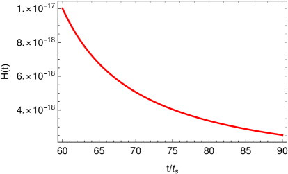
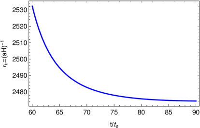
Figure 1: $Left~{}plot$ : $H(t)$ (along y-axis) vs. $\frac{t}{t_{s}}$ (along x-axis) for $6\times 10^{17}\leq t\leq 9\times 10^{17}\mathrm{sec.}$ The Hubble parameter along the y-axis is in the unit of sec^-1. $Right~{}plot$ : $r_{h}^{(l)}(t)$ (along y-axis) vs. $\frac{t}{t_{s}}$ for $6\times 10^{17}\leq t\leq 9\times 10^{17}$ sec, where the Hubble radius is in the unit of sec. The decreasing behavior of $r_{h}^{(l)}(t)$ clearly indicates an accelerating stage of the Universe during late time.

Fig.[1] clearly reveals that the Hubble radius decreases with time and leading to an accelerating stage of the Universe at late time. Therefore as a whole, the $F(R)$ (12) successfully provides a viable dark energy model in respect to Sne-Ia+BAO+H(z)+CMB data where the evolution of the Hubble parameter and the Hubble radius are given in Fig.[1]. Moreover, here it may be mentioned that the exponential $F(R)$ model has a Schwarzschild de-Sitter solution in the regime $R\gg\Lambda\sim 10^{-84}\mathrm{GeV}^{2}$. For example, in the Solar System regime $R^{*}\simeq 10^{-78}\mathrm{GeV}^{2}$, the exponential $F(R)$ model can be approximated as $F(R^{*})=R^{*}-2\Lambda$ (note that $R^{*}$ is greater than the $\Lambda$) and thus in this case, the Schwarzschild de-Sitter solution can be obtained, which is indeed a stable solution as depicted by some of our authors in Elizalde:2010ts .

Therefore Eqs.(11) and (12) represent the $F(R)$ gravity in the two situations, one depicting the early bounce of the Universe where the scale factor behaves as $a(t)=1+\alpha t^{2}$ ($=a_{b}(t)$) and the other providing a late time accelerating phase when the scale factor ($a_{l}(t)$) or more explicitly the Hubble parameter $H_{l}(t)$ goes according to the Fig.[1] (the corresponding scale factor can be easily obtained by using $a_{l}(t)=e^{\int H_{l}(t)dt}$). Till now, we have described the bounce and the dark energy (DE) era in a disjoint manner i.e $F_{b}(R)$ describes the Universe near the bounce but not the whole cosmological epochs, while the $F_{l}(R)$ reveals the behavior only at present time. Thus the immediate question that springs to mind is, what is the form of $F(R)$ for the entire range of cosmic time, which will further demonstrate the unification of bounce and dark energy era followed by a deceleration stage in the intermediate region? As a deceleration era, we may consider a matter dominated epoch in between the bounce and the present era. With this consideration, in Sec.[V], we will reconstruct the full $F(R)$ gravity, however numerically, by taking the forms of $F_{b}(R)$ and $F_{l}(R)$ as boundary conditions. In the method of numerical reconstruction, we need an appropriate scale factor (or equivalently Hubble radius) describing the Universe evolution for a wide range of cosmic time. For this purpose, we may consider an ansatz of the scale factor as follows,

$$a(t) = e^{\alpha t^{2}}\tanh{\bigg{[}\beta_{1}\bigg{(}1-\frac{t}{t_{p}}\bigg{)}\bigg{(}1-\frac{t}{t_{I}}\bigg{)}\bigg{]}}+\bigg{(}\frac{t}{T}\bigg{)}^{2/3}\tanh{\bigg{[}\beta_{2}\bigg{(}\frac{t}{t_{b}}-1\bigg{)}\bigg{(}1-\frac{t}{t_{p}}\bigg{)}\bigg{]}}$$ (15)

$$+ a_{l}(t)\tanh{\bigg{[}\beta_{3}\bigg{(}\frac{t}{t_{b}}-1\bigg{)}\bigg{(}\frac{t}{t_{I}}-1\bigg{)}\bigg{]}}$$

where $t_{b}$ is the bouncing time or even the horizon crossing time, $t_{p}$ is the present time instance and $t_{I}$ is an intermediate time. The above scale factor behaves as $a_{b}(t)=1+\alpha t^{2}$ near $t\simeq t_{b}\ll t_{I}\ll t_{p}$ i.e near the bounce, however goes as $a_{I}(t)=\big{(}t/T\big{)}^{2/3}$ near $t_{b}\ll t=t_{I}\ll t_{p}$ and as $a_{l}(t)=e^{\int H_{l}(t)dt}$ near the present time i.e $t\simeq t_{p}$. The parameters $\beta_{i}$ can be fixed by considering the corresponding hyperbolic tangent function tending to unity at the respective time.

Though the scale factor (15) provides the correct evolution of the universe near the bounce and at the late stage and also at a certain instance of the intermediate stage ($t\simeq t_{I}$), but it does not lead to correct evolution of the universe for the whole intermediate epoch. Thus to address the universe evolution smoothly for a wide range of cosmic time, we may consider $a(t)$ as,

$$a(t) = 1+\alpha t^{2}=a_{b}(t)~{}~{},~{}~{}~{}~{}~{}~{}~{}~{}~{}~{}~{}~{}~{}~{}~{}~{}~{}~{}~{}~{}~{}~{}~{}~{}~{}near~{}the~{}bounce,~{}for~{}~{}~{}~{}~{}~{}~{}t\simeq 0^{+}$$

$$a(t) = \bigg{(}\frac{t}{T}\bigg{)}^{2/3}=a_{I}(t)~{}~{},~{}~{}~{}~{}~{}~{}~{}in~{}the~{}intermediate~{}regime,~{}for~{}~{}~{}~{}~{}~{}~{}0^{+}\lesssim t\lesssim 5\times 10^{17}~{}sec$$

$$a(t) = e^{\int H_{l}(t)dt}=a_{l}(t)~{}~{},~{}~{}~{}~{}~{}~{}~{}~{}~{}~{}~{}~{}~{}~{}~{}~{}~{}~{}~{}~{}~{}during~{}late~{}time,~{}for~{}~{}~{}~{}~{}~{}~{}~{}t\gtrsim 6\times 10^{17}~{}sec$$ (16)

(with $T$ being an arbitrary parameter with dimension $sec$) and the transition from the bounce to the matter dominated and from matter dominated to the dark energy era will be obtained by the method of numerical interpolation. However, the process of interpolation requires appropriate choices for the values of the free parameters present in our model. It may be observed that there are three parameters hanging around in the theory, $\alpha$, $\Lambda$ and $\beta$. The parameter $\alpha$ appears from the near-bounce scale factor and thus can be named as “early stage parameter”, while $\Lambda$ and $\beta$ appear during the reconstruction in the late-time and thus the name - “late stage parameters”. The late stage parameters have been already estimated in view of the viability of the exponential $F(R)$ as a successful dark energy model. However, the early stage parameter $\alpha$ is still remaining to be determined and in the next section, we will estimate $\alpha$ from the latest Planck 2018 observational results.

IV Cosmological perturbation: Estimation of early stage parameters

Being the early stage parameter, $\alpha$ can be determined from various primordial observable quantities like the scalar spectral index ($n_{s}$), the tensor-to-scalar ratio ($r$) by directly confronting their theoretical expectations with the Planck 2018 observations. In this section, we consider the spacetime fluctuations over the FRW metric and consequently calculate various observable quantities like the scalar spectral index and tensor-to-scalar ratio. In a bouncing Universe, the primordial perturbation modes (relevant to the present day observation) generate either near the bounce or at a distant past far away from the bouncing point, depending upon the late-time behavior of the Hubble radius. Thereby before moving to the explicit perturbation calculation, it is important to analyze when the perturbation modes generate in the present context of bouncing Universe. In all the bouncing models, the Hubble parameter becomes zero and thus the comoving Hubble radius, defined by $r_{h}=\frac{1}{aH}$ (where $H$ is the Hubble parameter), diverges at the bouncing point. However, the asymptotic behavior of the comoving Hubble radius makes a difference in various bouncing models. In this regard, (1) for some bouncing scale factors, the Hubble radius decreases monotonically at both sides of the bounce and finally shrinks to zero size asymptotically, which corresponds to an accelerating late-time Universe. Therefore, in such cases, the Hubble horizon goes to zero at large values of the cosmic time, and only for cosmic times near the bouncing point the Hubble horizon has an infinite size. So the primordial perturbation modes relevant for present time era generate for cosmic times near the bouncing point, because only at that time all the primordial modes are contained in the horizon. As the horizon shrinks, the modes exit the horizon and become relevant for present time observations. On the other hand, (2) some bouncing scale factors lead to a divergent Hubble radius asymptotically, which corresponds to a decelerating Universe at late times. In such cases, the perturbation modes generate at very large negative cosmic times, corresponding to the low curvature regime of the contracting era, unlike to the previous situations, where the perturbation modes generate near the bouncing era. More explicitly, in the latter case, the comoving wave number $k$ begins its propagation through spacetime at large negative cosmic times, in the contracting phase on sub-Hubble scales, and exits the Hubble radius during this phase, and re-enters the Hubble radius during the low-curvature regime in expanding phase and thus being relevant for present time observations. Therefore, the physical picture in the two cases is very different with regard to when the perturbation modes generate. However as mentioned earlier, in the present work, we will deal with an unified scenario of bounce with late time acceleration connected by an intermediate deceleration epoch. Thus, the late-time Universe is characterized by an accelerating scale factor and hence the Hubble radius should shrink to zero asymptotically at both “sides” of the bounce (as the scale factor is considered to be symmetric around the bounce). This indicates that the perturbation modes generate near the bounce, rather than far away from the bouncing point, because near the bouncing regime the Hubble radius has an infinite size and all the perturbation modes are contained inside the horizon. Hence we solve the perturbation equations near the bounce i.e near $t=0$, which is the primary subject in the remaining part of this section.

IV.1 Scalar perturbation

In principle, perturbations should always be expressed in terms of gauge invariant quantities. In the present work, we shall work in the comoving gauge defined by the vanishing of the momentum density $\delta T_{0i}=0$ (where $T_{\mu\nu}$ is the effective energy-momentum tensor and the symbol ’$\delta$’ denotes the corresponding perturbation). In this gauge, the scalar metric perturbation is expressed as,

$$\delta g_{ij}=a^{2}(t)\big{[}1-2\Re\big{]}\delta_{ij}$$ (17)

where $\Re(t,\vec{x})$ denotes the scalar perturbation and known as the comoving curvature perturbation which is indeed a gauge invariant quantity. The additional metric perturbations $\delta g_{00}$ and $\delta g_{0i}$ can be obtained in terms of $\Re$ from perturbed gravitational equations and as a result, the second order action of $\Re(t,\vec{x})$ is given by Hwang:2005hb ; Noh:2001ia ; Hwang:2002fp ,

$$\delta S_{\Re}=\int dtd^{3}\vec{x}a(t)z(t)^{2}\left[\dot{\Re}^{2}-\frac{1}{a^{2}}\left(\partial_{i}\Re\right)^{2}\right]\,,$$ (18)

with $z(t)$ has the following expression,

$$z(t)=\frac{a(t)}{\kappa\bigg{(}H(t)+\frac{1}{2F^{\prime}(R)}\frac{dF^{\prime}(R)}{dt}\bigg{)}}\sqrt{\frac{3}{2F^{\prime}(R)}\bigg{(}\frac{dF^{\prime}(R)}{dt}\bigg{)}^{2}}$$ (19)

Eq.(18) clearly indicates that the sound speed of the scalar perturbation ($c_{s}^{2}$) is unity, which in turn guarantees the absence of superluminal modes or equivalently one may argue that the model is free from gradient instabilities. The unit sound speed for scalar perturbation is, in fact, a generic nature of $F(R)$ theory and also of a scalar-tensor theory. This equivalence, in respect of sound speed, between $F(R)$ and scalar tensor theory is however expected as both the theories can be mapped to one another (in the action level) by a conformal transformation of the metric. Coming back to the action (18), the scalar perturbation has positive kinetic terms if $z^{2}(t)>0$ holds, which is equivalent to the condition $F^{\prime}(R)>0$ as evident from Eq.(19). We will show that the $F(R)$ obtained in the earlier sections indeed satisfies $F^{\prime}(R)>0$ and ensures the stability of the scalar perturbation. The action $\delta S_{\Re}$ leads to the equation for the perturbed variable $\Re(\vec{x},t)$ as,

$$\frac{1}{a(t)z^{2}(t)}\frac{d}{dt}\bigg{[}a(t)z^{2}(t)\dot{\Re}\bigg{]}-\frac{1}{a^{2}}\partial_{i}\partial^{i}\Re=0$$ (20)

In terms of the Fourier transformed scalar perturbation variable $\Re_{k}(t)=\int d\vec{x}e^{-i\vec{k}.\vec{x}}\Re(\vec{x},t)$, the above equation can be written as,

$$\frac{1}{a(t)z^{2}(t)}\frac{d}{dt}\bigg{[}a(t)z^{2}(t)\dot{\Re}_{k}\bigg{]}+\frac{k^{2}}{a^{2}}\Re_{k}(t)=0$$ (21)

where $k$ is the wave number for the $k$-th perturbation mode. As mentioned earlier, we solve the above equation for cosmic times near the bouncing point as the perturbation modes themselves are generated close to the bounce and thereby we can use the form of $F(R)$ reconstructed in Eq.(11). With this expression of near-bounce-$F(R)$, we will determine $z(t)$ (an essential ingredient of perturbation equation (21)) and for this purpose, we first need to evaluate $F^{\prime}(R)$ and $F^{\prime\prime}(R)$ which are given by,

$$F^{\prime}(R)=\frac{12\alpha D}{\sqrt{e}}+\frac{D}{24}\bigg{[}-\frac{6\big{(}R-12\alpha\big{)}}{\sqrt{e}}+\frac{\sqrt{6\pi}e^{-\frac{R}{24\alpha}}\big{(}R-48\alpha\big{)}\sqrt{R-12\alpha}~{}Erfi\big{[}\frac{\sqrt{R-12\alpha}}{2\sqrt{6\alpha}}\big{]}}{2\sqrt{\alpha}}\bigg{]}$$ (22)

and

$$F^{\prime\prime}(R)=\frac{D}{576\alpha^{3/2}}\bigg{[}\frac{12\sqrt{\alpha}\big{(}R-72\alpha\big{)}}{\sqrt{e}}-\frac{\sqrt{6\pi}e^{-\frac{R}{24\alpha}}\big{(}R^{2}-96\alpha R+1440\alpha^{2}\big{)}~{}Erfi\big{[}\frac{\sqrt{R-12\alpha}}{2\sqrt{6\alpha}}\big{]}}{\sqrt{R-12\alpha}}\bigg{]}$$ (23)

respectively. Recall, the Ricci scalar scalar at the bounce becomes $R(0)=12\alpha$ and thus the function $Erfi\bigg{[}\frac{\sqrt{R-12\alpha}}{2\sqrt{6\alpha}}\bigg{]}$ can be expressed as Taylor series expansion in the powers of $\sqrt{R-12\alpha}$ near the bounce. However the terms with $\mathcal{O}((R-12\alpha)^{5/2})$ in the Taylor expansion can be neglected as such terms will eventually lead to a higher power of $t$ in comparison to $t^{2}$ and all the near-bounce quantities have been or will be evaluated up to $\mathcal{O}(t^{2})$, as we also did for the near-bounce scale factor in Sec.[III.1]. Using the Taylor expansion of $Erfi\bigg{[}\frac{\sqrt{R-12\alpha}}{2\sqrt{6\alpha}}\bigg{]}$ along with the expression of $R(t)$ (see Eq.(8)), we evaluate the $F^{\prime}(R)$ and $F^{\prime\prime}(R)$ up to $\mathcal{O}(t^{2})$ as follows,

$$F^{\prime}(R(t))=\frac{12\alpha D}{\sqrt{e}}-\frac{12\alpha D}{\sqrt{e}}~{}\alpha t^{2}$$ (24)

and

$$F^{\prime\prime}(R(t))=-\frac{1}{\alpha}\bigg{[}\frac{\alpha D}{\sqrt{e}}-\frac{4\alpha D}{3\sqrt{e}}~{}\alpha t^{2}\bigg{]}$$ (25)

respectively. Eq.(24) indicates that $F^{\prime}(R)$ is positive near the bounce and hence ensures the stability of the scalar perturbation. On other hand, $F^{\prime\prime}(R)$ becomes negative near the bounce, which is clear from Eq.(25). Actually the condition $F^{\prime\prime}(R)<0$ is connected with the violation of null energy condition in the $F(R)$ gravity theory and thus such condition should hold in order for a bounce to be generated, and the demonstration goes as follows: recall, as mentioned in Sec.[II] that the $F(R)$ gravity contributes an effective energy-momentum tensor where the effective energy density ($\rho_{eff}$) and the pressure ($p_{eff}$) are given in Eqs.(5) and (6) respectively. Using these expressions of $\rho_{eff}$ and $p_{eff}$ along with the Hubble factor $H(t)=2\alpha t$, it is easy to show that at the bounce $\rho_{eff}+p_{eff}$ becomes $=2\dot{H}\big{(}F^{\prime}(R(t))-1\big{)}+24\dot{H}^{2}F^{\prime\prime}(R(t))$. The $F^{\prime}(R)$ and $F^{\prime\prime}(R)$, as we obtained near $t=0$ in the present context, leads to $\rho_{eff}+p_{eff}<0$ i.e the violation of energy condition which in turn ensures a bouncing phenomena at $t=0$. Plugging the expressions of $F^{\prime}(R)$, $F^{\prime\prime}(R)$ into Eq.(19), we get,

$$a(t)z^{2}(t)=\frac{72\alpha D}{\kappa^{2}\sqrt{e}}\bigg{[}1+\frac{2}{3}\alpha t^{2}\bigg{]}=U_{1}+V_{1}~{}\alpha t^{2}$$ (26)

where $U_{1}=\frac{72\alpha D}{\kappa^{2}\sqrt{e}}$ and $V_{1}=\frac{48\alpha D}{\kappa^{2}\sqrt{e}}$. With the above expression of $a(t)z^{2}(t)$, the scalar perturbed equation (21) takes the following form,

$$U_{1}\ddot{\Re}_{k}+2\alpha V_{1}\dot{\Re}_{k}~{}t+k^{2}U_{1}\Re_{k}(t)=0$$ (27)

at leading order in $t$. Solving Eq.(27) for $\Re_{k}(t)$, we get,

$$\Re_{k}(t)=b_{1}(k)~{}e^{-\frac{V_{1}}{U_{1}}\alpha t^{2}}~{}H\bigg{[}-1+\frac{k^{2}}{2\alpha}\frac{U_{1}}{V_{1}},\sqrt{\frac{\alpha V_{1}}{U_{1}}}~{}t\bigg{]}$$ (28)

with $H[n,x]$ is the nth order Hermite polynomial. $b_{1}(k)$ is the integration constant which can be determined by the initial state of the canonical Mukhanov-Sasaki variable $v_{k}(t)$ defined by $v_{k}(t)=z(t)\Re_{k}(t)$, which is the adiabatic vacuum state. Thus near the bounce (i.e near $t\simeq 0$), the field $v_{k}(t)$ satisfies

$$\lim_{t\rightarrow 0}v_{k}=\frac{1}{\sqrt{2k}}e^{-ik\tau}$$ (29)

where $\tau$ is the conformal time defined by $d\tau=\frac{dt}{a(t)}$. However near $t\simeq 0$, the conformal and cosmic time become same as,

$$\tau=\int\frac{dt}{a(t)}=\int\frac{dt}{(1+\alpha t^{2})}\simeq t~{}~{}.$$

Furthermore for cosmic times that satisfy $t\simeq 0$, the Hubble horizon is infinitely large and thus the primordial modes are well inside the Hubble horizon i.e the perturbation modes satisfy $k\gg aH$. As a result, the equation for the field $v_{k}(t)$ becomes

$$\frac{d^{2}v_{k}}{d\tau^{2}}+k^{2}v_{k}=0~{}~{}.$$ (30)

This is the equation of a simple harmonic oscillator with time-independent frequency. For this case, the solution for the minimum energy state is given by $v_{k}=\frac{1}{\sqrt{2k}}e^{-ik\tau}$. Hence we impose the initial condition as shown in Eq.(29). This justifies the choice of the adiabatic vacuum state in the present context. On other hand, the function $H\bigg{[}-1+\frac{k^{2}U_{1}}{2\alpha V_{1}},\sqrt{\frac{\alpha V_{1}}{U_{1}}}t\bigg{]}$ has a limiting value for $t\rightarrow 0$ and is given by,

$$H\bigg{[}-1+\frac{k^{2}U_{1}}{2\alpha V_{1}},\sqrt{\frac{\alpha V_{1}}{U_{1}}}~{}t\bigg{]}\bigg{|}_{t\rightarrow 0}=\frac{2^{\frac{k^{2}U_{1}}{2\alpha V_{1}}}\sqrt{\pi}}{2\Gamma\big{(}1-\frac{k^{2}U_{1}}{4\alpha V_{1}}\big{)}}$$

with $\Gamma(z)$ symbolizes the “Gamma function“. Therefore, by considering the adiabatic vacuum as the initial condition of $\Re_{k}(t)$, the integration constant turns out to be,

$$b_{1}(k)=\frac{1}{z(t\rightarrow 0)}\bigg{[}\frac{2\Gamma\big{(}1-\frac{k^{2}U_{1}}{4\alpha V_{1}}\big{)}}{\sqrt{2\pi k}~{}2^{\frac{k^{2}U_{1}}{2\alpha V_{1}}}}\bigg{]}=\frac{1}{\sqrt{U_{1}}}\bigg{[}\frac{2\Gamma\big{(}1-\frac{k^{2}U_{1}}{4\alpha V_{1}}\big{)}}{\sqrt{2\pi k}~{}2^{\frac{k^{2}U_{1}}{2\alpha V_{1}}}}\bigg{]}$$ (31)

where in the second equality, we used $z(t\rightarrow 0)=\frac{1}{\sqrt{U_{1}}}$ from Eq.(26). Thus as a whole, the solution for the scalar perturbation variable becomes,

$$\Re_{k}(t) = \bigg{(}\frac{2\Gamma\big{(}1-\frac{k^{2}U_{1}}{4\alpha V_{1}}\big{)}}{\sqrt{2\pi k}~{}2^{\frac{k^{2}U_{1}}{2\alpha V_{1}}}\sqrt{U_{1}}}\bigg{)}~{}e^{-\frac{V_{1}}{U_{1}}\alpha t^{2}}~{}H\bigg{[}-1+\frac{k^{2}U_{1}}{2\alpha V_{1}},\sqrt{\frac{\alpha V_{1}}{U_{1}}}~{}t\bigg{]}$$ (32)

$$= \bigg{(}\frac{2\kappa~{}\Gamma\big{(}1-\frac{3k^{2}}{8\alpha}\big{)}}{\sqrt{2\pi k}~{}2^{\frac{3k^{2}}{4\alpha}}\sqrt{12\alpha D}}\bigg{)}~{}e^{\big{[}\frac{1}{4}-\frac{2}{3}\alpha t^{2}\big{]}}~{}H\bigg{[}-1+\frac{3k^{2}}{4\alpha},\sqrt{\frac{2\alpha}{3}}~{}t\bigg{]}$$

where we have used $U_{1}=\frac{72\alpha D}{\kappa^{2}\sqrt{e}}$ and $V_{1}=\frac{48\alpha D}{\kappa^{2}\sqrt{e}}$ in the second equality. Consequently, the above solution of $\Re_{k}(t)$ immediately leads to the scalar power spectrum for $k$-th mode as follows,

$$P_{\Re}(k,t) = \frac{k^{3}}{2\pi^{2}}~{}\bigg{|}\Re_{k}(t)\bigg{|}^{2}$$ (33)

$$= \frac{k^{2}}{12\alpha D\pi^{3}}~{}\frac{\bigg{(}\kappa~{}\Gamma\big{(}1-\frac{3k^{2}}{8\alpha}\big{)}\bigg{)}^{2}}{~{}2^{\frac{3k^{2}}{2\alpha}}~{}}e^{\big{[}\frac{1}{2}-\frac{4}{3}\alpha t^{2}\big{]}}~{}\bigg{\{}H\bigg{[}-1+\frac{3k^{2}}{4\alpha},\sqrt{\frac{2\alpha}{3}}~{}t\bigg{]}\bigg{\}}^{2}$$

Using the horizon crossing relation $k=aH$, the scalar power spectrum can be expressed in terms of the quantities at horizon crossing as,

$$P_{\Re}(k,t)\bigg{|}_{h.c}=\frac{\alpha t_{h}^{2}}{3D\pi^{3}}~{}\frac{\bigg{(}\kappa~{}\Gamma\big{(}1-\frac{3\alpha t_{h}^{2}}{2}\big{)}\bigg{)}^{2}}{~{}2^{6\alpha t_{h}^{2}}~{}}e^{\big{[}\frac{1}{2}-\frac{4}{3}\alpha t_{h}^{2}\big{]}}~{}\bigg{\{}H\bigg{[}-1+3\alpha t_{h}^{2},\sqrt{\frac{2\alpha}{3}}~{}t_{h}\bigg{]}\bigg{\}}^{2}$$ (34)

where $t_{h}$ is the horizon crossing time. With Eq. (33), we can determine the spectral index of the primordial curvature perturbations. However before proceeding to calculate the spectral index, we will perform first the tensor perturbation, which is necessary for evaluating the tensor-to-scalar ratio.

IV.2 Tensor perturbation

Let us now focus on the tensor perturbations, and the tensor perturbation on the FRW metric background is defined as follows,

$$ds^{2}=-dt^{2}+a(t)^{2}\left(\delta_{ij}+h_{ij}\right)dx^{i}dx^{j}\,,$$ (35)

where $h_{ij}(t,\vec{x})$ is the tensor perturbation. The variable $h_{ij}(t,\vec{x})$ is itself a gauge invariant quantity, and the tensor perturbed action up to quadratic order is given by,

$$\delta S_{h}=\int dtd^{3}\vec{x}a(t)z_{T}(t)^{2}\left[\dot{h}_{ij}\dot{h}^{ij}-\frac{1}{a^{2}}\left(\partial_{l}h_{ij}\right)^{2}\right]\,,$$ (36)

where $z_{T}(t)$ has the following form Hwang:2005hb ,

$$z_{T}(t)=\frac{a(t)}{\kappa}\sqrt{F^{\prime}(R)}\,,$$ (37)

Therefore the speed of the tensor perturbation is $c_{T}^{2}=1$ i.e the gravitational waves propagate with the speed of light which is unity in the natural units.

Coming back to Eq.(37), the stability of the tensor perturbation will be guaranteed by the condition $F^{\prime}(R)>0$ - the same condition by which the scalar perturbation is ensured to be stable. Recall, in the previous section, we showed the positivity of $F^{\prime}(R)$ in Eq. (24) and thus the tensor perturbation is indeed stable in the present context. The action (36) leads to the equation of the tensor perturbed variable as,

$$\frac{1}{a(t)z_{T}^{2}(t)}\frac{d}{dt}\bigg{[}a(t)z_{T}^{2}(t)\dot{h}_{ij}\bigg{]}-\frac{1}{a^{2}}\partial_{l}\partial^{l}h_{ij}=0$$ (38)

The Fourier transformed tensor perturbation variable is defined as $h_{ij}(t,\vec{x})=\int d\vec{k}~{}\sum_{\gamma}\epsilon_{ij}^{(\gamma)}~{}h_{(\gamma)}(\vec{k},t)e^{i\vec{k}.\vec{x}}$, where $\gamma=^{\prime}+^{\prime}$ and $\gamma=^{\prime}\times^{\prime}$ represent two polarization modes. Moreover $\epsilon_{ij}^{(\gamma)}$ are the polarization tensors satisfying $\epsilon_{ii}^{(\gamma)}=k^{i}\epsilon_{ij}^{(\gamma)}=0$. In terms of the Fourier transformed tensor variable $h_{k}(t)$, Eq.(38) can be expressed as,

$$\frac{1}{a(t)z_{T}^{2}(t)}\frac{d}{dt}\bigg{[}a(t)z_{T}^{2}(t)\dot{h}_{k}\bigg{]}+\frac{k^{2}}{a^{2}}h_{k}(t)=0$$ (39)

The two polarization modes obey the same Eq.(39) and thus we omit the polarization index. Moreover, both the polarization modes even follow the same initial condition and that is why they have the same solution. So in the following, what we will do in the context of tensor perturbation is applicable for both the polarization modes. Finally, in the expression of the tensor power spectrum, we will introduce a multiplicative factor $2$ due to the contribution from both the polarization modes. Using the expression of $F^{\prime}(R)$ from Eq.(24), we determine $a(t)z_{T}^{2}(t)$ as,

$$a(t)z_{T}^{2}(t)=\frac{12\alpha D}{\kappa^{2}\sqrt{e}}\bigg{[}1+2\alpha t^{2}\bigg{]}=U_{2}+V_{2}~{}\alpha t^{2}$$ (40)

with $U_{2}=\frac{12\alpha D}{\kappa^{2}\sqrt{e}}$ and $V_{2}=\frac{24\alpha D}{\kappa^{2}\sqrt{e}}$. Plugging back this expression of $a(t)z_{T}^{2}(t)$ into Eq.(39) and after some algebra, we get the following equation,

$$U_{2}\ddot{h}_{k}+2\alpha V_{2}\dot{h}_{k}~{}t+k^{2}U_{2}h_{k}(t)=0$$ (41)

at leading order in $t$, which is a viable consideration because the perturbation modes generate near the bouncing phase in the present scenario. Solving Eq.(41) for $h_{k}(t)$ , we get,

$$h_{k}(t)=b_{2}(k)~{}e^{-\frac{V_{2}}{U_{2}}\alpha t^{2}}~{}H\bigg{[}-1+\frac{k^{2}}{2\alpha}\frac{U_{2}}{V_{2}},\sqrt{\frac{V_{2}}{U_{2}}\alpha}~{}t\bigg{]}$$ (42)

where $b_{2}(k)$ is an integration constant and can be determined from an initial condition. As an initial condition, we consider that the tensor perturbation field starts from the adiabatic vacuum, more precisely the initial configuration is given by, $\lim_{t\rightarrow 0}\big{[}z_{T}(t)h_{k}(t)\big{]}=\frac{1}{\sqrt{2k}}$. This immediately leads to the expression of $b_{2}(k)$ as,

$$b_{2}(k)=\frac{1}{z_{T}(t\rightarrow 0)}\bigg{[}\frac{2\Gamma\big{(}1-\frac{k^{2}U_{2}}{4\alpha V_{2}}\big{)}}{\sqrt{2\pi k}~{}2^{\frac{k^{2}U_{2}}{2\alpha V_{2}}}}\bigg{]}=\frac{1}{\sqrt{U_{2}}}\bigg{[}\frac{2\Gamma\big{(}1-\frac{k^{2}U_{2}}{4\alpha V_{2}}\big{)}}{\sqrt{2\pi k}~{}2^{\frac{k^{2}U_{2}}{2\alpha V_{2}}}}\bigg{]}~{}~{}~{}.$$ (43)

In the second equality of the above equation, we use $z_{T}(t\rightarrow 0)=1/\sqrt{U_{2}}$ from Eq.(40). Plugging this expression of $b_{2}(k)$ into Eq.(42) yields the final solution of $h_{k}(t)$ as follows,

$$h_{k}(t) = \bigg{(}\frac{2\Gamma\big{(}1-\frac{k^{2}U_{2}}{4\alpha V_{2}}\big{)}}{\sqrt{2\pi k}~{}2^{\frac{k^{2}U_{2}}{2\alpha V_{2}}}\sqrt{U_{2}}}\bigg{)}~{}e^{-\frac{V_{2}}{U_{2}}\alpha t^{2}}~{}H\bigg{[}-1+\frac{k^{2}U_{2}}{2\alpha V_{2}},\sqrt{\frac{V_{2}}{U_{2}}\alpha}~{}t\bigg{]}$$ (44)

$$= \bigg{(}\frac{2\kappa~{}\Gamma\big{(}1-\frac{k^{2}}{8\alpha}\big{)}}{\sqrt{2\pi k}~{}2^{\frac{k^{2}}{4\alpha}}\sqrt{12\alpha D}}\bigg{)}~{}e^{\big{[}\frac{1}{4}-2\alpha t^{2}\big{]}}~{}H\bigg{[}-1+\frac{k^{2}}{4\alpha},\sqrt{2\alpha}~{}t\bigg{]}$$

where we have used $U_{2}=\frac{12\alpha D}{\kappa^{2}\sqrt{e}}$ and $V_{2}=\frac{24\alpha D}{\kappa^{2}\sqrt{e}}$. Eq.(44) represents the solution of the tensor perturbation for both the polarization modes. The solution of $h_{k}(t)$ immediately leads to the tensor power spectrum as,

$$P_{h}(k,t) = \frac{k^{3}}{2\pi^{2}}~{}\sum_{\gamma}\bigg{|}h_{k}^{(\gamma)}(t)\bigg{|}^{2}$$ (45)

$$= \frac{k^{2}}{6\alpha D\pi^{3}}~{}\frac{\bigg{(}\kappa~{}\Gamma\big{(}1-\frac{k^{2}}{8\alpha}\big{)}\bigg{)}^{2}}{~{}2^{\frac{k^{2}}{2\alpha}}}e^{\big{[}\frac{1}{2}-4\alpha t^{2}\big{]}}~{}\bigg{\{}H\bigg{[}-1+\frac{k^{2}}{4\alpha},\sqrt{2\alpha}~{}t\bigg{]}\bigg{\}}^{2}$$

It may be noticed that $\gamma=^{\prime}+^{\prime}$ and $\gamma=^{\prime}\times^{\prime}$ modes contribute equally to the power spectrum, as expected because their solutions behave similarly. At the horizon crossing, the tensor power spectrum turns out to be,

$$P_{h}(k,t)\bigg{|}_{h.c}=\frac{2\alpha t_{h}^{2}}{3D\pi^{3}}~{}\frac{\bigg{(}\kappa~{}\Gamma\big{(}1-\frac{\alpha t_{h}^{2}}{2}\big{)}\bigg{)}^{2}}{~{}2^{2\alpha t_{h}^{2}}}e^{\big{[}\frac{1}{2}-4\alpha t_{h}^{2}\big{]}}~{}\bigg{\{}H\bigg{[}-1+\alpha t_{h}^{2},\sqrt{2\alpha}~{}t_{h}\bigg{]}\bigg{\}}^{2}$$ (46)

Now we can explicitly confront the model at hand with the latest Planck observational data Akrami:2018odb , so we shall calculate the spectral index of the primordial curvature perturbations $n_{s}$ and the tensor-to-scalar ratio $r$, which are defined as follows,

$$n_{s}-1=\frac{\partial\ln{P_{\Re}}}{\partial\ln{k}}\bigg{|}_{H.C}~{}~{}~{}~{}~{}~{}~{}~{},~{}~{}~{}~{}~{}~{}~{}~{}~{}~{}~{}r=\frac{P_{h}(k,t)}{P_{\Re}(k,t)}\bigg{|}_{H.C}$$ (47)

As evident from these expressions, $n_{s}$ and $r$ are evaluated at the time of the first horizon exit near the bouncing point, for positive times (symbolized by ’H.C’ in the above equations), when $k=aH$ i.e. when the mode $k$ crosses the Hubble horizon. Using Eq.(33), we determine $\frac{\partial\ln{P_{\Re}}}{\partial\ln{k}}$ as follows,

$$\frac{\partial\ln{P_{\Re}}}{\partial\ln{k}}=2-\frac{3k^{2}}{2\alpha}~{}\psi^{(0)}\bigg{[}1-\frac{3k^{2}}{8\alpha}\bigg{]}-\frac{3k^{2}}{\alpha}(\ln{2})+\frac{3k^{2}}{\alpha}\bigg{\{}\frac{H^{(1,0)}\bigg{[}-1+\frac{3k^{2}}{4\alpha},\sqrt{\frac{2\alpha}{3}}~{}t\bigg{]}}{H\bigg{[}-1+\frac{3k^{2}}{4\alpha},\sqrt{\frac{2\alpha}{3}}~{}t\bigg{]}}\bigg{\}}$$ (48)

where $\psi^{(0)}[z]$ is the zeroth order Polygamma function or equivalently the digamma function and $H^{(1,0)}[z_{1},z_{2}]$ is the derivative of $H[z_{1},z_{2}]$ with respect to its first argument. Moreover the following expressions were used to calculate Eq.(48),

$$\frac{\partial}{\partial k}\bigg{\{}\Gamma\bigg{(}1-\frac{3k^{2}}{8\alpha}\bigg{)}\bigg{\}} = -\frac{3k}{4\alpha}~{}\Gamma\bigg{(}1-\frac{3k^{2}}{8\alpha}\bigg{)}~{}\psi^{(0)}\bigg{(}0,1-\frac{3k^{2}}{8\alpha}\bigg{)}$$

$$\frac{\partial}{\partial k}\bigg{\{}H\bigg{[}-1+\frac{3k^{2}}{4\alpha},\sqrt{\frac{2\alpha}{3}}~{}t\bigg{]}\bigg{\}} = \frac{3k}{2\alpha}~{}H^{(1,0)}\bigg{[}-1+\frac{3k^{2}}{4\alpha},\sqrt{\frac{2\alpha}{3}}~{}t\bigg{]}$$ (49)

Thereby Eq.(48) immediately leads to the spectral index as,

$$n_{s}=\bigg{[}3-\frac{3k^{2}}{2\alpha}~{}\psi^{(0)}\bigg{(}0,1-\frac{3k^{2}}{8\alpha}\bigg{)}-\frac{3k^{2}}{\alpha}(\ln{2})+\frac{3k^{2}}{2\alpha}\bigg{\{}\frac{H^{(1,0)}\bigg{(}-1+\frac{3k^{2}}{4\alpha},\sqrt{\frac{2\alpha}{3}}~{}t\bigg{)}}{H\bigg{(}-1+\frac{3k^{2}}{4\alpha},\sqrt{\frac{2\alpha}{3}}~{}t\bigg{)}}\bigg{\}}\bigg{]}_{H.C}$$ (50)

As mentioned earlier, the perturbation modes are generated and also cross the horizon near the bounce. Thus we can safely use the near-bounce scale factor in the horizon crossing condition to determine $k=aH=2\alpha t_{h}$ (where $t_{h}$ is the horizon crossing time). Using this relation, Eq.(50) turns out to be,

$$n_{s}=3-6\alpha t_{h}^{2}~{}\psi^{(0)}\bigg{(}0,1-\frac{3}{2}~{}\alpha t_{h}^{2}\bigg{)}-12\alpha t_{h}^{2}(\ln{2})+12\alpha t_{h}^{2}\bigg{\{}\frac{H^{(1,0)}\bigg{(}-1+3\alpha t_{h}^{2},\sqrt{\frac{2\alpha}{3}}~{}t_{h}\bigg{)}}{H\bigg{(}-1+3\alpha t_{h}^{2},\sqrt{\frac{2\alpha}{3}}~{}t_{h}\bigg{)}}\bigg{\}}$$ (51)

Furthermore, the tensor-to-scalar ratio is given by,

$$r=\bigg{|}\frac{h_{k}(t)}{\Re_{k}(t)}\bigg{|}^{2}_{k=a(t_{h})H(t_{h})}$$ (52)

where the solutions of $h_{k}(t)$ and $\Re_{k}(t)$ are shown in Eqs.(44) and (32) respectively. Eqs.(51) and (52) clearly indicate that $n_{s}$ and $r$ depend on the dimensionless parameter $\alpha t_{h}^{2}$ which is further connected to the Ricci scalar at horizon crossing by $\alpha t_{h}^{2}=\big{(}\frac{R_{h}}{12\alpha}-1\big{)}$. Thereby, we can argue that the observable quantities $n_{s}$ and $r$ depend on $R_{h}/\alpha$. With this information, we now directly confront the theoretical expectations of spectral index and tensor-to-scalar ratio with the Planck 2018 constraints Akrami:2018odb . In Fig. [2] we present the estimated spectral index and tensor-to-scalar ratio of the present scenario for three choices of $\frac{R_{h}}{\alpha}$, on top of the $1\sigma$ and $2\sigma$ contours of the Planck 2018 results Akrami:2018odb . As we observe, the agreement with observations is efficient, and in particular well inside the $1\sigma$ region. At this stage it is worth mentioning that in an $F(R)$ gravity theory, the matter bounce scenario, in which case the perturbations are generated far away from the bouncing point deeply in the contracting regime, is not consistent with the Planck results as shown in Odintsov:2014gea . However, here we demonstrate that a $F(R)$ gravity model indeed leads to a viable bouncing model where the primordial perturbations are generated near the bounce. Thereby, we can argue that the viability of a $F(R)$ model (with respect to the Planck constraints) is interrelated with the generation era of the perturbations modes.

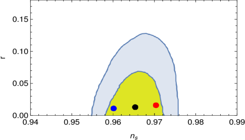
Figure 2: $1\sigma$ (yellow) and $2\sigma$ (light blue) contours for Planck 2018 results Akrami:2018odb , on $n_{s}-r$ plane. Additionally, we present the predictions of the present bounce scenario with $\frac{R_{h}}{\alpha}=14$ (blue point), $\frac{R_{h}}{\alpha}=16$ (black point) and $\frac{R_{h}}{\alpha}=20$ (red point).

Furthermore the scalar perturbation amplitude ($A_{s}$) is constrained by $\ln{\big{[}10^{10}A_{s}\big{]}}=3.044\pm 0.014$ due to the Planck results Akrami:2018odb . Eq.(33) along with the consideration of the integration constant $D=\frac{1}{\alpha}$ (recall $D$ has mass dimension [-2]) depict that the scalar perturbation amplitude depends on the dimensionless parameters $\frac{{R_{h}}}{\alpha}$ and $\alpha\kappa^{2}$. We may choose $\frac{R_{h}}{\alpha}=16$ (which is within the range that makes the $n_{s}$ and $r$ compatible with the Planck results) and consequently the scalar perturbation amplitude in the present context becomes $A_{s}=\frac{1}{20\pi^{3}}\alpha\kappa^{2}$. Therefore the theoretical expectation of $A_{s}$ will match with the Planck observations provided $\alpha\kappa^{2}$ lies within $\alpha\kappa^{2}=[1.283\times 10^{-7},1.320\times 10^{-7}]$. Thus as a whole, the observable quantities $n_{s}$, $r$ and $A_{s}$ are simultaneously compatible with the Planck constraints for the parameter ranges : $14\leq\frac{R_{h}}{\alpha}\leq 20$ and $\alpha\kappa^{2}=[1.283\times 10^{-7},1.320\times 10^{-7}]$ respectively. However the viable range of $\alpha\kappa^{2}$ depends on the consideration $D=1/\alpha$, i.e. a different $D$ will eventually lead to a different range of viability of the parameter $\alpha\kappa^{2}$. As an example, for $D=\frac{1}{4\alpha}$, the scalar perturbation amplitude becomes $A_{s}=\frac{1}{5\pi^{3}}\alpha\kappa^{2}$ while $n_{s}$ and $r$ have the same form as given in Eqs.(51) and (52) respectively and therefore the parameters should lie within $14\leq\frac{R_{h}}{\alpha}\leq 20$ and $\alpha\kappa^{2}=[3.208\times 10^{-8},3.300\times 10^{-8}]$ in order to make the theoretical values of the observable quantities compatible with the latest Planck 2018 results. Such parametric ranges make the horizon crossing Ricci scalar of the order $R_{h}\sim 10^{-8}/\kappa^{2}=10^{28}\mathrm{GeV}^{2}$.

Thereby, the viable ranges of the early and late stage parameters are given by $14\lesssim\frac{R_{h}}{\alpha}\lesssim 20$, $\alpha\kappa^{2}=[3.208\times 10^{-8},3.300\times 10^{-8}]$, $\beta=3.98^{+\infty}_{-2.46}$ and $\Lambda=1.2\times 10^{-84}\mathrm{GeV}^{2}$ respectively. As a result, we can interpolate the scale factor or the Hubble radius in the two transition eras (i.e from the bounce to matter dominated and from the matter dominated to dark energy epoch), leading to a smooth evolution of the Hubble radius for a large range of cosmic time.

Before moving to the next section we would like to mention that in the present context, the non-singular bounce universe is time symmetric and the initial adiabatic vacuum condition is set at the bouncing point, which seems that the model is more similar to a scenario of the creation of the universe from nothing. The spontaneous birth of the universe from “nothing” has been discussed earlier in the context of quantum cosmology where the universe is described by a wave function satisfying the well known Wheeler-DeWitt equation Halliwell:1990uy . With the development of quantum cosmology theory, it has been suggested that the universe can be created spontaneously from nothing, where “nothing” means there is neither matter nor space or time, and the problem of singularity can be avoided naturally Atkatz:1994hy ; He:2014yia . In particular, the author of Atkatz:1994hy showed that a quantum universe of zero size, or, indeed, the cosmological “nothing” may quantum mechanically tunnel to a universe of a finite size. However the argument of Atkatz:1994hy was established for a closed type universe, unlike to the present bounce scenario which has been presented for a flat FRW universe.

V Numerical solutions: An unified description from bounce-to-deceleration-to-late time acceleration

Given the structure of the scale factor in the early and late stages of the Universe (as $a_{b}(t)=1+\alpha t^{2}$ in Eq.(7) and $a_{l}(t)=e^{\int H_{l}(t)dt}$ respectively, where the $H_{l}(t)$ is given in Fig.[1]), we would like to provide a complete picture by considering the intermediate region to be a matter dominated epoch, and moreover the transitions from the bounce to matter dominated (MD) and from the matter dominated to the DE era will be obtained by the method of numerical interpolation. Due to complicated nature of the equations governing the evolution of the scale factor in a general context, we will determine the interpolating function using numerical techniques and will illustrate the same. Let us briefly point out the methods one may use in order to generate such interpolating solutions. In the transition regions (i.e. from the bounce-MD and from the MD-DE), one approximates the behavior of the physical quantity of interest (e.g., the scale factor $a(t)$ or the Hubble radius $r_{h}=\frac{1}{aH}$) by a polynomial function of time, with degree of the polynomial kept arbitrary. Then, in the early bounce epoch one uses the given behavior of the desired physical quantity (for example for the scale factor, the behavior near the bounce is $a_{b}(t)=1+\alpha t^{2}$) to generate numerical estimates of the respective quantity at various time instants till the description is reliable. Similar numerical estimations are being made at the intermediate matter dominated and at the late stage as well. With these sets of data and the polynomial function one can use any standard interpolation software package to end up getting the desired plots. The structure of the plot, of course, depends on the degree of the polynomial and desired accuracy level. All the plots in this paper are for an accuracy level of $\mathcal{O}(10^{-8})$. Since our main aim is to merge certain cosmological epochs of the Universe, a good physical quantity to start with is the Hubble radius ($r_{h}(t)$) rather than the scale factor, because the accelerating or decelerating stage of the Universe is easily realized by the decreasing or increasing behavior of the Hubble radius (with respect to cosmic time) respectively. Following Eq.(16), we may construct the Hubble radius as,

$$r_{h}(t) = \big{[}\dot{a}_{b}(t)\big{]}^{-1}=\frac{1}{2\alpha t}~{}~{},~{}~{}~{}~{}~{}~{}~{}~{}~{}~{}~{}~{}~{}~{}~{}~{}~{}~{}~{}~{}~{}~{}~{}~{}~{}~{}~{}~{}~{}~{}~{}~{}near~{}the~{}bounce,~{}for~{}~{}~{}~{}~{}~{}~{}t\simeq 0^{+}$$

$$r_{h}(t) = \big{[}\dot{a}_{I}(t)\big{]}^{-1}=\frac{3t}{2}\bigg{(}\frac{T}{t}\bigg{)}^{2/3}~{}~{},~{}~{}~{}~{}~{}~{}~{}in~{}the~{}intermediate~{}regime,~{}for~{}~{}~{}~{}~{}~{}~{}0^{+}\lesssim t\lesssim 5\times 10^{17}~{}sec.$$

$$r_{h}(t) = \big{[}\dot{a}_{l}(t)\big{]}^{-1}~{}~{}~{}(see~{}Fig.[\ref{plot_rec_late}])~{}~{},~{}~{}~{}~{}~{}~{}~{}~{}~{}~{}~{}~{}~{}~{}~{}~{}~{}~{}~{}~{}~{}during~{}late~{}time,~{}for~{}~{}~{}~{}~{}~{}~{}~{}t\gtrsim 6\times 10^{17}~{}sec.$$ (53)

and then with the procedure described above, we numerically interpolate the Hubble radius in the two transitions i.e. from the bounce to matter dominated and from the matter dominated to DE era respectively. Moreover the Hubble radius in the contracting regime can also be obtained by assuming a symmetric behavior of $\big{|}r_{h}(t)\big{|}$ around the bounce. However, the details of the interpolation of the curve connecting the early bounce to the late accelerating stage is an artifact of the procedure followed and admits possible variations depending on the process of interpolation by numerical techniques. However such indeterminacy in determining the interpolating function would not affect our main conclusions in the present context. Thus, having explained the details of the interpolating procedure, we now turn to the corresponding implications and present the variations of all the relevant parameters with time.

As mentioned earlier, we start with the Hubble radius ($r_{h}=\frac{1}{\dot{a}}$), in particular, taking the reduced Planck mass to be $M_{\mathrm{Pl}}=10^{18}\mathrm{GeV}$ and using the aforementioned construction of the Hubble radius, we obtain $r_{h}(t)$ as a function of time in the expanding phase of the Universe. Further the Hubble radius in the contracting regime is obtained by considering a symmetric character of $\big{|}r_{h}(t)\big{|}$ in the both sides of the bounce. As a result, we get the Hubble radius for $-9\times 10^{17}\leq t\leq 9\times 10^{17}$ sec., which is presented in the left part of Fig.[3], while the right part is a zoomed-in version of the left one near $t=0$. The x-axis of the Fig.[3] corresponds to a “rescaled” time coordinate obtained as $\frac{t}{t_{s}}$ (with $t_{s}=10^{16}$ sec.) which is dimensionless, while the $y$ axis represents the rescaled Hubble radius $\bar{r}_{h}=10^{-5}r_{h}$ which is in the unit of “sec”. Fig.[3] clearly demonstrates that the Hubble radius depicts a bounce at $t=0$ (as expected, because it is constructed from $r_{h}^{(b)}(t)=\big{(}a_{b}H_{b}\big{)}^{-1}$ near $t=0$), then it increases monotonically with time up to $\frac{t}{t_{s}}\simeq 50$ (or $t=5\times 10^{17}$ sec.) leading to a decelerating phase of the Universe and finally after $t\gtrsim 5\times 10^{17}$ sec., the Hubble radius starts to decrease, which in turn indicates the dark energy epoch of the Universe. This may provide a merging of a non-singular bounce to matter dominated epoch, followed by a late time dark energy era. It may be noticed that the Hubble radius goes to zero asymptotically at both “sides” of the bounce, which in turn confirms the fact that the relevant primordial perturbation modes generate near the bouncing point as we have considered in Sec.[IV] during the calculation of scalar and tensor perturbations. The generation era of perturbation modes in the present context makes the model different than the usual matter bounce scenario where the perturbation modes generate in the distant past far away from the bounce.

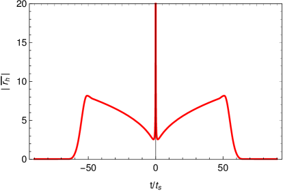
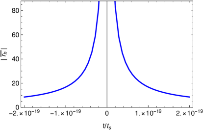
Figure 3: $Left~{}plot$ : The modulus of the rescaled Hubble radius $\big{|}\bar{r}_{h}\big{|}$ (along y-axis, in the unit of second) is being plotted against $\frac{t}{t_{s}}$ (along x-axis) for a wide range of cosmic time, in particular for $-9\times 10^{17}\leq t\leq 9\times 10^{17}$ sec. Such construction of the Hubble radius depends on Eq.(53) and the numerical interpolation in the transition eras i.e from the bounce-MD and the MD-dark energy epoch. During numerical interpolation, we take $\alpha\kappa^{2}=3.25\times 10^{-8}$, $\beta=4$ and $T=1$ sec. The curve explicitly shows a smooth unification of the Universe evolution from the bounce-to-deceleration-to-late time acceleration. $Right~{}plot$ : A zoomed-in version of the left plot near $t=0$.

Having this Hubble radius, we are now going to solve the scale factor and Hubble parameter, however numerically and then by using the numerical solution of $H(t)$ we reconstruct the form of $F(R)$ from the gravitational Eq.(4). The scale factor can be obtained from $\dot{a}(t)=\frac{1}{r_{h}(t)}$ which is a first order differential equation and thus the solution of the same requires one boundary condition. We choose $a(0)=1$, because we want the scale factor to behave like $a_{b}(t)$ near $t=0$ and recall $a_{b}(0)=1$. With such initial condition along with the $r_{h}(t)$ given in Fig.[3], we solve $a(t)$ numerically, which is presented in Fig.[4] where once again, the x axis is rescaled by $t_{r}=t/t_{s}$.

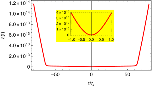
Figure 4: $a(t)$ (along y-axis) vs. $\frac{t}{t_{s}}$ (along x-axis). The scale factor gets a minimum at $t=0$ and thus indicates a non-singular bounce at that point of time. To get a better view of what is happening near the bounce, we give a zoomed-in version by the inset-graph depicting the behavior of the scale factor near $t=0$.

It is evident that the scale factor is smooth everywhere and the graph in the inset shows that the scale factor acquires a minimum at $t=0$. Thus we can argue that the Universe transits from a contracting phase to an expanding one through a non-singular bounce at $t=0$ and thus the Universe evolution becomes free of the initial singularity. The above numerical solutions of the scale factor can be immediately differentiated providing the Hubble parameter as a function of time, shown in Fig.[5].

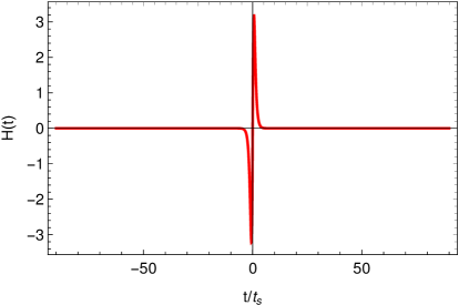
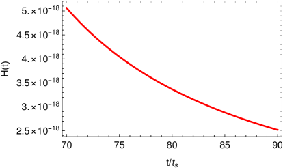
Figure 5: $Left~{}plot$ : $H(t)$ (along y-axis, in the unit of sec^-1) vs. $\frac{t}{t_{s}}$ (along x-axis) for $-9\times 10^{17}\leq t\leq 9\times 10^{17}$ sec., which is obtained from the solution of the scale factor shown in Fig.[4]. As evident, $H(t)$ becomes zero at $t=0$ and $\dot{H}(0)>0$, confirming a bouncing Universe. Moreover the Hubble parameter acquires a maximum near the bounce. Finally in the late time epoch, the Hubble parameter monotonically decreases with time. $Right~{}plot$ : A zoomed-in version of $H(t)$ vs. $\frac{t}{t_{s}}$ for $7\times 10^{17}\leq t\leq 9\times 10^{17}$ sec.

The Hubble parameter becomes zero and shows an increasing behavior with time (i.e $\dot{H}>0$) at $t=0$, however this is expected as the scale factor itself acquires a minimum at $t=0$ i.e. a bounce. Moreover, the Hubble parameter acquires a maximum very near to bounce and then decreases rapidly, and continued to decrease until the late-time era. A zoomed-in version of the late time behavior of $H(t)$ is shown in the right plot of Fig. [5], which clearly demonstrates that at the late epoch i.e. for $t\gtrsim 7\times 10^{17}$ sec., the Hubble parameter becomes of the order $\sim 10^{-18}$ sec^-1. The occurrence of the maximum of $H(t)$ near the bounce in the present context is in agreement with Odintsov:2016tar where the authors explained the merging of bounce with late-time acceleration from a different viewpoint, namely from the holonomy generalizations of $deformed$ matter bounce scenario. In this regard, it may be mentioned that a deformed matter bounce scenario is represented by an asymmetric scale factor where the Hubble radius diverges at $t\rightarrow-\infty$ and asymptotically goes to zero at $t\rightarrow+\infty$. Thus the primordial perturbation modes in a deformed matter bounce model generate deeply in the contracting regime far away from the bounce, unlike to our present case where the Hubble radius goes to zero asymptotically at both “sides” of the bounce (see Fig.[3]) leading to the generation of the perturbation modes near the bouncing regime.

With the Hubble parameter at hand, our next task is to solve the gravitational equation (4) to reconstruct the form of $F(R)$ which can realize such evolution of the Hubble parameter. For this purpose, we need two boundary conditions as Eq.(4) is a second order differential equation with respect to the Ricci scalar. As mentioned earlier, we use the forms of $F_{b}(R)$ and $F_{l}(R)$ obtained in Sec.[III] for such boundary conditions and thus the boundary conditions are given by: $F(R=0)=F_{l}(0)$ and $F(R_{b}=12\alpha)=F_{b}(12\alpha)$ respectively (recall, $R_{b}$ is the Ricci scalar at the bounce). As a result, we solve Eq. (4) numerically and the form of $F(R)$ we get is depicted in the left part of Fig.[6]. Actually the $F(R)$ is demonstrated by the red curve, while the yellow one represents the Einstein gravity.

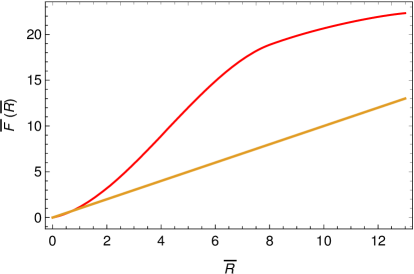
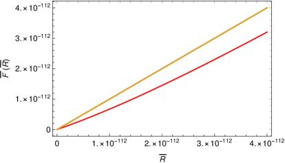
Figure 6: $Left~{}plot$ : $\bar{F}(\bar{R})$ (along y axis) vs. $\bar{R}$ (along x axis). The red curve depicts the numerical solution of the $F(R)$ and the yellow curve represents the Einstein gravity. The figure reveals that the $F(R)$ matches with the Einstein gravity in the low curvature regime, while the $F(R)$ seems to deviate from the usual General Relativity when the scalar curvature takes larger and larger values $Right~{}plot$ : A zoomed-in version of the left plot near $R\rightarrow 0$ to get a better view of the behaviour of the $F(R)$ during the present epoch.

Before going into the discussion regarding the behavior of the $F(R)$ gravity, let us briefly comment about the range of the “rescaled Ricci scalar” that we take along the x-axis in Fig.[6]. Recall, the Ricci scalar near the bounce gets the value $R(t\rightarrow 0)\simeq 12\alpha$ where the parameter $\alpha$ lies within $[3.208\times 10^{-8}/\kappa^{2},3.300\times 10^{-8}/\kappa^{2}]$ to make the primordial observable quantities compatible with the Planck constraints. Thereby, the Ricci scalar near the bounce becomes of the order $\sim 12\times 10^{28}\mathrm{GeV}^{2}$, while in the present epoch, the scalar curvature is generally considered to take $10^{-84}\mathrm{GeV}^{2}$. Thus in order to correctly describe the epochs from bounce to late time acceleration, we have to cover the range of $R(t)$ from $\sim 12\times 10^{28}\mathrm{GeV}^{2}$ to $10^{-84}\mathrm{GeV}^{2}$. However in Fig.[6], we consider a “rescaled Ricci scalar” given by $\bar{R}=\frac{R}{\alpha}$ along the x-axis, which is dimensionless as $\alpha$ has the mass dimension [+2]. Due to such rescaling, the x-axis of the plot runs from the value $x_{i}=10^{-112}$ (or we may take $x_{i}=0$) to $x_{f}=12$. Moreover, the y-axis of Fig.[6] is also rescaled by $\bar{F}(\bar{R})=F(R)/\alpha$ so that the Einstein gravity can be described by a straight line having slope of unity even in these rescaled coordinates. The left part of the Fig. [6] clearly demonstrates that the solution of $F(R)$ matches with the Einstein gravity as the Ricci scalar approaches to the present value, while the $F(R)$ seems to deviate from the usual Einstein gravity, when the scalar curvature takes larger and larger values. It is evident that near the bounce, $F^{\prime}(R)$ is positive, which in turn indicates the stability for the scalar and tensor perturbations. This finding from the numerical solution, in fact, resembles with the analytic results obtained in Sec.[IV]. The comparison of $F(R)$ gravity with the Einstein one in the low-curvature regime is explicitly demonstrated in the right part of Fig.[5], which reveals that the form of $F(R)$ reconstructed in the present context is indeed comparable with Einstein gravity during the present epoch. Thus, we can safely argue that the numerical solution of $F(R)$ obtained above indeed matches with the analytic results determined near the bounce and at the dark energy era.

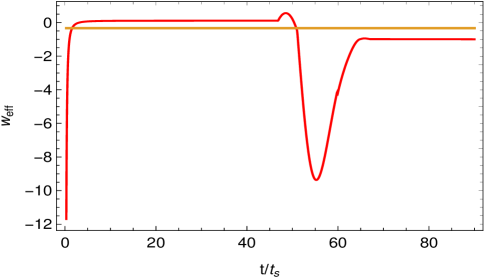
Figure 7: $w_{eff}$ (along y axis) vs. $\frac{t}{t_{s}}$ (along x axis) for $0\lesssim t\leq 9\times 10^{17}$ sec. The red curve represents the $w_{eff}$ for the present model while the yellow one is for the constant value $-\frac{1}{3}$. Thereby the successive crossing between the red and yellow curves depicts the transition of the Universe from acceleration to deceleration or vice-versa.

Using the form of $F(R)$ and the Hubble parameter from Fig.[6] and [5] respectively, we determine the remaining bit i.e the effective equation of state (EoS) parameter defined by,

$$w_{eff}=\frac{\bigg{[}\frac{f(R)}{2}-\big{(}3H^{2}+\dot{H}\big{)}f^{\prime}(R)+6\big{(}8H^{2}\dot{H}+4\dot{H}^{2}+6H\ddot{H}+\dddot{H}\big{)}f^{\prime\prime}(R)+36\big{(}4H\dot{H}+\ddot{H}\big{)}^{2}f^{\prime\prime\prime}(R)\bigg{]}}{\bigg{[}-\frac{f(R)}{2}+3\big{(}H^{2}+\dot{H}\big{)}f^{\prime}(R)-18\big{(}4H^{2}\dot{H}+H\ddot{H}\big{)}f^{\prime\prime}(R)\bigg{]}}~{}~{},$$

as shown in Fig. [7], where the x-axis is the rescaled time coordinate i.e $\frac{t}{t_{s}}$ with $t_{s}=10^{16}$ sec. Actually the red curve of the plot represents the $w_{eff}$ for the present model while the yellow one is for the constant value $-\frac{1}{3}$ (we will keep the yellow graph to investigate the accelerating or decelerating era of the Universe). Fig.[7] clearly demonstrates that at the bounce i.e. at $t=0$, the EoS parameter diverges from the negative side, however this is expected because at the bounce the Hubble parameter itself becomes zero and in turn makes the $w_{eff}=-1-\frac{2\dot{H}}{3H^{2}}\rightarrow-\infty$. Then immediately after the bounce, $w_{eff}$ crosses the value $-\frac{1}{3}$ leading to a transition from a bounce to a decelerating phase of the Universe, and during the deceleration epoch, the EoS parameter remains almost constant and near to zero indicating a quasi-matter dominated Universe which continues till $t\simeq 5\times 10^{17}$ sec, when the EoS parameter again crosses the value $-\frac{1}{3}$ and thus the Universe transits from a stage of deceleration to a stage of acceleration continued until the late-time era. Therefore, the present model may provide an unified scenario of certain cosmological epochs from bounce to late-time acceleration followed by a quasi-matter dominated epoch in the intermediate regime. Moreover, the EoS parameter during the dark energy era approaches to the value $-0.995$, as evident from the Fig.[7]. This late time value of the $w_{eff}$ is, however, in agreement with Elizalde:2010ts where the authors considered the exponential $F(R)$ as a dark energy model, similar to the present case.

VI Logarithmic corrected exponential $F(R)$ gravity as dark energy model: A different $F(R)$ for unification of bounce and late time acceleration

In this section, we consider a different $F(R)$ dark energy model in comparison to the one we considered in the previous sections, in particular, we incorporate an additional logarithmic correction to the exponential $F(R)$ gravity. Thus the form of $F(R)$ is given by Odintsov:2018qug ,

$$F(R)=R-2\Lambda\bigg{(}1-e^{-\frac{\beta R}{2\Lambda}}\bigg{)}\bigg{[}1-\frac{\gamma R}{2\Lambda}~{}\log{\big{(}\frac{R}{4\Lambda}\big{)}}\bigg{]}$$ (54)

where the correction over Einstein gravity is given by

$$F(R)-R=-2\Lambda\bigg{(}1-e^{-\frac{\beta R}{2\Lambda}}\bigg{)}\bigg{[}1-\frac{\gamma R}{2\Lambda}~{}\log{\big{(}\frac{R}{4\Lambda}\big{)}}\bigg{]}~{}~{}.$$

It may be observed that such correction goes to zero at $R\rightarrow 0$ i.e in the low curvature regime. Now in order to avoid including an implicit cosmological constant in a $F(R)$ model or equivalently to avoid the fine tuning problem associated with the cosmological constant, the correction over the Einstein-Hilbert term of the $F(R)$ gravity requires to vanish in the low curvature limit i.e

$$\lim_{R\rightarrow 0}\big{(}F(R)-R\big{)}=0~{}~{}.$$ (55)

As just mentioned, this condition is satisfied for the considered $F(R)$ model in Eq.(54) and thus this $F(R)$ model can produce the vacuum solution as the Minkowski spacetime. Thereby we may argue that the model (54) is free from the problem of including an implicit cosmological constant, unlike to the scenario with the action given by $S=\int d^{4}x\sqrt{-g}\big{[}R-2\Lambda\big{]}$. The condition (55) for avoiding a cosmological constant is also satisfied for the exponential $F(R)$ gravity as considered earlier in Eq.(12) i.e without the logarithmic corrections. However as described in Odintsov:2018qug , the presence of the logarithmic correction, modelled by the free parameter $\gamma$ by Eq.(54), leads to a better fit (in respect to a viable dark energy model) than in absence of the logarithmic correction and also better than the $\Lambda\mathrm{CDM}$ model. Hence the inclusion of the logarithmic correction provides a test for this type of $F(R)$ theory and motivates to check how a deviation is allowed in comparison to the $\Lambda\mathrm{CDM}$ model. Note that the logarithmic correction introduces a new parameter $\gamma$ i.e for $\gamma=0$, the $F(R)$ model (54) becomes similar to the exponential model considered earlier in Eq.(12). This new $F(R)$ model with the logarithmic term still satisfies the viability conditions (under some conditions of the free parameter) and provides an extra term in the action that evolutes smoothly along the cosmological evolution (far from the pole obviously), as addressed in the Ref. Odintsov:2018qug . In particular, the logarithmic corrected exponential $F(R)$ gravity comes as a viable dark energy model with respect to the Sne-Ia+BAO+H(z)+CMB data for the parametric choices : $\gamma=0.0014^{+0.0025}_{-0.0014}$, $\Lambda=1.2\times 10^{-84}\mathrm{GeV}^{2}$ and $\beta=4.71^{+\infty}_{-2.87}$ respectively. Such parametric regimes makes the $F(R)$ model free from antigravity effects due to the condition $\gamma\log{\big{(}\frac{R}{4\Lambda}\big{)}}<1$ holds true. The authors of Odintsov:2018qug clearly investigated the possible effects of the logarithmic term on the dark energy epoch in view of the aforementioned observational data and as a result, they found that the logarithmic correction modelled by the parameter $\gamma$ leads to better fit than in the absence of logarithmic correction (i.e. the pure exponential $F(R)$ model), obviously at the price of introducing a new parameter $\gamma$. Moreover the model (54) avoids the presence of large corrections on the Newton’s law as well as the appearance of large instabilities at local systems, leading to a suitable model that recovers the well known results of General Relativity at the appropriate scales. In view of this new dark energy model, we propose the following $F(R)$ gravity,

$$F(R)=R - 2\Lambda\bigg{(}1-e^{-\frac{\beta R}{2\Lambda}}\bigg{)}\bigg{[}1-\frac{\gamma R}{2\Lambda}~{}\log{\big{(}\frac{R}{4\Lambda}\big{)}}\bigg{]}+\exp{\bigg{\{}1-\cosh{\bigg{(}\frac{R}{R_{b}}+\frac{R_{b}}{R}-2\bigg{)}}\bigg{\}}}$$ (56)

$$\bigg{[} \bigg{(}\frac{12\alpha D}{\sqrt{e}}-1-\gamma\log{\big{(}\frac{R}{4\Lambda}\big{)}}\bigg{)}R-D\sqrt{6\alpha\pi}~{}e^{-\frac{R}{24\alpha}}\big{(}R-12\alpha\big{)}^{3/2}~{}Erfi\big{[}\frac{\sqrt{R-12\alpha}}{2\sqrt{6\alpha}}\big{]}\bigg{]}$$

which can merge the bounce and late-time acceleration as we will show in the following, where the late time behavior is described by the $F(R)$ of Eq.(54) and the bouncing scenario is still depicted by the $F_{b}(R)$ determined in Eq.(11). In the above expression, the $R_{b}$ denotes the scalar curvature at the bounce i.e $R_{b}=12\alpha\sim 10^{28}\mathrm{GeV}^{2}$ (see Sec. [IV] for the estimation of $\alpha$). We introduce an additional cosine hyperbolic factor (let us call it “fixing factor“) with the second term of the right hand side of Eq.(56) in order to avoid the effects of the second term during the late-time era. With the above $F(R)$, the demonstration of universe’s evolution at different curvature regimes goes as follows: (1) for $R\gg\Lambda$ when the Ricci scalar is given by $R(t)=12\alpha+12\alpha^{2}t^{2}$ (i.e near the bounce), the cosine hyperbolic term behaves as,

$$\cosh{\bigg{(}\frac{R}{R_{b}}+\frac{R_{b}}{R}-2\bigg{)}}=\cosh{\bigg{(}\frac{\alpha^{2}t^{4}}{(1+\alpha t^{2})}\bigg{)}}=\frac{1}{2}\big{[}e^{\frac{\alpha^{2}t^{4}}{(1+\alpha t^{2})}}+e^{-\frac{\alpha^{2}t^{4}}{(1+\alpha t^{2})}}\big{]} = 1+\frac{\alpha^{4}t^{8}}{2(1+\alpha t^{2})^{2}}+.........$$

$$= 1+\mathcal{O}(t^{8})$$

and therefore the fixing factor can be expressed by $e^{-\mathcal{O}(t^{8})}=1-\mathcal{O}(t^{8})$. However, recall that the near bounce quantities are determined up to $\mathcal{O}(t^{2})$ and thus the factor $e^{-\mathcal{O}(t^{8})}$ can be approximated to unity near $R\simeq R_{b}$. As a result along with the fact $R_{b}\gg\Lambda$, the $F(R)$ of Eq.(56) turns out to be,

$$F(R)=\frac{12\alpha D}{\sqrt{e}}R-D\sqrt{6\alpha\pi}~{}e^{-\frac{R}{24\alpha}}\big{(}R-12\alpha\big{)}^{3/2}Erfi\bigg{[}\frac{\sqrt{R-12\alpha}}{2\sqrt{6\alpha}}\bigg{]}=F_{b}(R)$$ (57)

in the regime $R\simeq R_{b}$, which realizes a bouncing Universe as discussed in Sec. [III.1]. However in order to ensure a bounce, it is also necessary to check $F^{\prime}(R)$ and $F^{\prime\prime}(R)$ as they are connected to the issues of energy conditions. Being the evolution of the fixing factor as $e^{-\mathcal{O}(t^{8})}=1-\mathcal{O}(t^{8})$ and since $\frac{dR}{dt}$ is proportional to $t$ around the bounce, one can immediately write $F^{\prime}(R)=F_{b}^{\prime}(R)$ and $F^{\prime\prime}(R)=F_{b}^{\prime\prime}(R)$ up to $\mathcal{O}(t^{2})$ near $R\simeq R_{b}$. Thereby, the $F(R)$ we propose in Eq.(56) as well as its first and second derivatives match with that of $F_{b}(R)$ up to $\mathcal{O}(t^{2})$, which clearly indicates a bouncing Universe for $R\simeq R_{b}$. Here it may be mentioned that a different fixing factor like $e^{-\big{(}\frac{R}{R_{b}}+\frac{R_{b}}{R}-2\big{)}}$ behaves as $1+\mathcal{O}(t^{4})$ near the regime $R\simeq R_{b}$, unlike to our considered fixing factor where the leading order is proportional to $t^{8}$ due to the additional cosine hyperbolic term. However in effect of fourth order term (i.e $t^{4}$) being the leading order one, the fixing factor $e^{-\big{(}\frac{R}{R_{b}}+\frac{R_{b}}{R}-2\big{)}}$ makes the $F^{\prime}(R)$ different in comparison to $F_{b}^{\prime}(R)$ even up to $\mathcal{O}(t^{2})$, which in turn may violate the bounce at $R\simeq R_{b}$. In view of these arguments, we stick to the “fixing factor” as proposed in Eq.(56) rather than $e^{-\big{(}\frac{R}{R_{b}}+\frac{R_{b}}{R}-2\big{)}}$. On other hand, (2) for $R\ll R_{b}$ i.e in the low curvature regime (or equivalently $R\sim\Lambda$), $\frac{R_{b}}{R}$ becomes very much larger in comparison to $\frac{R}{R_{b}}$ and as a consequence the factor $\exp{\bigg{\{}1-\cosh{\bigg{(}\frac{R}{R_{b}}+\frac{R_{b}}{R}-2\bigg{)}}\bigg{\}}}$ can be approximated to $\exp{\big{[}-e^{R_{b}/R}\big{]}}$ which further tends to zero in the regime $\frac{R}{R_{b}}\ll 1$. Thereby, in the low curvature regime, the form of $F(R)$ can be written as $F(R)=R-2\Lambda\bigg{(}1-e^{-\frac{\beta R}{2\Lambda}}\bigg{)}\bigg{[}1-\frac{\gamma R}{2\Lambda}~{}\log{\big{(}\frac{R}{4\Lambda}\big{)}}\bigg{]}$ leading to a viable dark energy dominated era in respect to Sne-Ia+BAO+H(z)+CMB observations for a suitable parametric spaces, as mentioned earlier. Moreover the $F(R)$ model (56) satisfies $\lim_{R\rightarrow 0}\big{(}F(R)-R\big{)}=0$ i.e the correction over the Einstein-Hilbert term vanishes in the limit $R\rightarrow 0$. This indicates that the $F(R)$ of Eq.(56) is able to provide the Minkowski solution in vacuum case and thus is free from the problem of including an implicit cosmological constant. Thus, the $F(R)$ proposed in Eq. (56) appropriately provides a non-singular bounce and a late acceleration near $R\simeq R_{b}$ and during $R\sim\Lambda$ respectively, and hence is able to merge a bounce with dark energy (DE) epoch. The deceleration stage in between the bounce and the dark energy epochs can be obtained by the numerical interpolation, similarly as we did for the earlier case in Sec.[V].

At this stage it deserves mentioning that we have taken the bottom-up approach to reconstruct the $F(R)$ gravity in the present context, in which we attempt to figure out the functional form of $F(R)$ by demanding that it should explain the observational results. However, various terms in the $F(R)$ of Eq.(56) may be thought to have a fundamental origin, like - near the bouncing regime, the $F(R)$ (denoted by $F_{b}(R)$) is given by Eq.(57). Thereby if we expand the Taylor series of the function $Erfi\bigg{[}\frac{\sqrt{R-12\alpha}}{2\sqrt{6\alpha}}\bigg{]}$ (present in Eq.(57)) around the bouncing point i.e around $R=12\alpha$ and keeping the leading order term, then the near-bounce expression of $F(R)$ will contain linear and quadratic power in curvature $R$. Such quadratic correction in the Ricci scalar plays a role for renormalizability of General Relativity (GR) in quantum gravity. On other hand, during the late time, the $F(R)$ behaves as of Eq.(54). The logarithmic correction present in the late time form of $F(R)$ may be thought as one-loop effects of quantum gravity. Despite these arguments, it is true that due to the complicated nature of the full $F(R)$ presented in Eq.(56), it is hard to realize some fundamental origin of this full form of $F(R)$. Of course, the complete gravitational action should be defined by a fundamental theory, which, however, remains to be the open problem of modern high-energy physics. In the absence of fundamental quantum gravity, the modified gravity approach in this work is a phenomenological one that is constructed by complying with observational data.

Before concluding, we would like to mention that the present scenario merges certain cosmological epochs of the universe, in particular, from a non-singular bounce to a matter dominated epoch and from the matter dominated to a late time accelerating epoch; i.e the model is similar to a matter bounce model which is also compatible to a late dark energy phase of the cosmic evolution as well. However this is not the full evolution history of the universe mainly due to the absence of the radiation era. Thereby in order to unify the entire evolutionary epochs of the universe in the context of bouncing cosmology, one should show the unification of an early bounce with the radiation domination, followed by the photon decoupling, followed by matter domination, all the way to the late-time dominance of dark energy stage. The unification for the full evolution of the universe is a longstanding problem in cosmology and we hope that our present paper may enlighten some part(s) of this bigger problem.

VII Conclusion

In the present work, we proposed a cosmological model in the context of $F(R)$ gravity, which merges a non-singular bounce to a matter dominated epoch and from the matter dominated to a late time accelerating epoch; i.e the model is similar to a generalized matter bounce model which is also compatible to a late dark energy dominant phase of the cosmic evolution. Using the reconstruction schemes, we reconstructed the form of $F(R)$ near the bounce and at the late-time era respectively. However, the reconstruction techniques applied in these two eras are slightly different, in particular: near the bouncing regime, we first considered a scale factor (suitable for bounce) and then determined the form of $F(R)$ which can realize such bouncing scale factor by using the gravitational equation of motion, while on other hand in the case of late times, we have used a reverse reconstruction procedure in comparison to that of the earlier one i.e. we started with a form of $F(R)$ (rather than a scale factor) viable for dark energy model, namely the exponential $F(R)$ gravity, and then reconstructed the corresponding Hubble parameter from the gravitational equations of motion. During such reconstructions, we got early and late stage model parameters which have been estimated from various observational constraints. The early stage parameters have been obtained from the primordial perturbations and we confronted the theoretical results of the observable quantities like the scalar spectral index, the tensor-to-scalar ratio with the latest Planck 2018 constraints. On other hand, the late stage parameters are estimated by investigating the viability of the exponential $F(R)$ gravity as a dark energy model with respect to the Sne-Ia+BAO+H(z)+CMB data. Due to a late accelerating phase, the Hubble radius decreases monotonically at late times and asymptotically goes to zero, which in turn leads to the generation of the primordial perturbation near the bounce (because at that time the relevant perturbation modes are within the horizon), unlike to the usual matter bounce scenario where the perturbation modes generate deeply in the contracting regime far away from the bouncing point time. Thus we have performed the perturbations near the bounce and as a result the primordial observable quantities like the spectral index for curvature perturbation, and the tensor-to-scalar ratio, are found to be simultaneously compatible with the latest Planck 2018 observations. Moreover, the scalar and tensor perturbations are stable as the condition $F^{\prime}(R)>0$ holds in the present context. With the early bounce and the late accelerating phase, we provided a complete evolution of the Hubble radius by considering the intermediate region to be a matter dominated epoch and the transitions from the bounce to matter dominated and from the matter dominated to the DE era have been obtained by the method of numerical interpolation, where the estimated values of the model parameters are incorporated. The evolution of the Hubble radius provides the universe’s evolution for a considerable range of cosmic time, in particular, it merges a non-singular bounce to a matter dominated epoch, followed by a late time accelerating stage. With this interpolating Hubble radius, we have numerically solved the $F(R)$ gravitational equation to determine the form of $F(R)$ for a wide range of cosmic time, which clearly depicts that the $F(R)$ matches with the Einstein gravity in the low curvature regime, while it deviates from the usual Einstein gravity as the scalar curvature acquires larger and larger values. Correspondingly, the Hubble parameter and the effective EoS parameter of the Universe have been determined. As a result the EoS parameter is found to successively cross the value $-\frac{1}{3}$ twice indicating the transition of the Universe from bounce to a quasi-matter dominated phase and from the quasi-matter dominated to a late-time accelerating stage respectively. Moreover, the EoS parameter during the dark energy era approaches to the value $-0.995$. Finally, in Sec. [VI], we have proposed a different $F(R)$ gravity form which is able to merge a non-singular bounce with a dark energy epoch, however the DE epoch is described by a logarithmic corrected exponential $F(R)$ gravity, unlike to the earlier case where the dark energy model is depicted by the usual exponential $F(R)$ gravity i.e. without the logarithmic corrections. Similar to the exponential $F(R)$ model, the logarithmic generalized exponential $F(R)$ gravity is also known to provide a viable dark energy model with respect to Sne-Ia+BAO+H(z)+CMB observations, in fact, the presence of logarithmic corrections leads to a better fitted model than the usual exponential $F(R)$ model.