Multistability and rare spontaneous transitions in barotropic $\beta$-plane turbulence

Abstract

We demonstrate that turbulent zonal jets, analogous to Jovian ones, which are quasi-stationary, are actually metastable. After extremely long times, they randomly switch to new configurations with a different number of jets. The genericity of this phenomenon suggests that most quasi-stationary turbulent planetary atmospheres might have many climates and attractors for fixed values of the external forcing parameters. A key message is that this situation will usually not be detected by simply running the numerical models, because of the extremely long mean transition time to change from one climate to another. In order to study such phenomena, we need to use specific tools: rare event algorithms and large deviation theory. With these tools, we make a full statistical mechanics study of a classical barotropic beta-plane quasigeostrophic model. It exhibits robust bimodality with abrupt transitions. We show that new jets spontaneously nucleate from westward jets. The numerically computed mean transition time is consistent with an Arrhenius law showing an exponential decrease of the probability as the Ekman dissipation decreases. This phenomenology is controlled by rare noise-driven paths called instantons. Moreover, we compute the saddles of the corresponding effective dynamics. For the dynamics of states with three alternating jets, we uncover an unexpectedly rich dynamics governed by the symmetric group ${\cal S}_{3}$ of permutations, with two distinct families of instantons, which is a surprise for a system where everything seemed stationary in the hundreds of previous simulations of this model. We discuss the future generalization of our approach to more realistic models.

1 Introduction

Many complex physical and natural systems have more than one local attractor. The dynamics can then settle close to one of these local attractors for a very long time, and randomly switch to another one. Well-known examples are phase transitions in condensed matter or conformational change of molecules in biochemistry (Maragliano et al., 2010). Such situations of multistability are ubiquitous also in geophysics and for turbulent flows (Ravelet et al., 2004; Bouchet and Simonnet, 2009). The reversal of the Earth magnetic field on geological timescales, which is due to turbulent motion of the Earth’s metal core (Berhanu et al., 2007), is a paradigmatic example.

The climate system is no exception and global multistability and abrupt transitions existed from the global Neoproterozoic glaciations (snowball Earth events) (Pierrehumbert et al., 2011) to glacial-interglacial cycles of the Pleistocene (Paillard, 1998). Very often, those transitions are due to the internal dynamics and are not caused by changes of external parameters. This is the case for instance for the fast Dansgaard–Oeschger events (Dansgaard et al., 1993; Ditlevsen et al., 2007; Rahmstorf, 2002). More local multistabilities also exist in part of the climate system, for instance the Kuroshio bimodality (Schmeits and Dijkstra, 2001; Qiu and Miao, 2000) in the North Pacific.

If multistability and abrupt transitions between distinguishable states are generic features of complex dynamical systems, why should planetary atmosphere dynamics be an exception? Actually Lorenz was already raising this question in 1967 (Lorenz, 1967). The hypothesis of a transition to a superrotating atmosphere with eastward equatorial jets has been addressed many times (Held, 1999) and observed in many numerical experiments (Arnold et al., 2012). Recently the more specific question of an abrupt transition to superrotation has been studied carefully (Herbert et al., 2020). On Earth, superrotation may have played a role in the climate of the past: it was observed in numerical simulations of warm climates such as the Eocene (Caballero and Huber, 2010), and it has been suggested that it could explain the permanent El Niño conditions indicated by paleoclimatic proxies during the Pliocene (Tziperman and Farrell, 2009).

The aim of this paper is to address the hypothesis of planetary atmosphere multistability and abrupt transitions not for equatorial jets but for midlatitude eddy-driven jets. This is a natural hypothesis as multiple midlatitude jets are observed on many planets, and that even with Earth conditions slight changes of parameters lead to a different number of jets (Lee, 1997, 2005) and jets of different nature (Kaspi and Flierl, 2007). Because it is difficult to change from a state with $n$ zonal jets, to a state with $n+1$ zonal jets continuously, it is natural to expect multistability, abrupt transitions, and spontaneous transitions between those different states to be generic.

A striking aspect of Jovian jets is their stability. Despite the strong turbulent activity at small scales, one hardly notices any difference between the two separate measurements by Voyager and Cassini 20 years apart (see Fig.1). The Jovian large-scale atmosphere, including the Great Red Spot, in fact appears to be stationary for decades. However, a fantastic event occurred in 1939-1940 when Jupiter lost one of its jets (Rogers, 1995). Three white anticyclones were created which started to merge in the late 90s into a large white anticyclone (see Fig.1). As such, Marcus (2004) called the 1939–1940 event a global climate change on Jupiter. The mechanism responsible for the disappearance of one of the jet remains completely unknown.

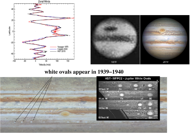
Figure 1: Upper left panel: Jupiter’s zonally averaged zonal velocity profile observed by Voyager, Cassini (Porco et al., 2004) and Hubble (Simon et al., 2015). Upper right panel: Great Red Spot contraction after one century (left: from (Clerke, 1893), right: NASA). Lower panel: three white ovals appeared in 1939-1940 (Rogers, 1995) and later merged to from the oval BA, also called ”Red Spot Junior” in 2006 when it turned red.

A key scientific aspect of bistability situations is that the time scale for observing a spontaneous transition from one attractor to another can be extremely long. For instance on Jupiter, no such events as the 1939-1940 jet disappearance occurred since then. The typical timescale for observing such transitions is thus longer than 80 years, while energy balance for jet-mean flow interactions, Rossby wave dynamics, and radiative effects have time scales much smaller ranging from one Jupiter day to several years. For this reason, we argue in this paper that most of time, scientists running numerical simulations are not aware that their model may have more than one attractor, just because they never simulate it long enough. Actually, simulating the model long enough and waiting, is most of the time impossible with currently available computational capabilities. This time-scale separation issue seems an impassable barrier. Breaking this constraint and studying unobserved phenomenologies for such transitions are two fascinating scientific aims. For instance in this paper, we will demonstrate that a barotropic model of self organized jets has a huge number of climate (attractors) for a fixed set of boundary conditions and forcing parameters, with an amazingly rich long-time dynamical structure for the transitions from one attractor to another. This was completely unexpected and never observed, even if analogous models have been run by many investigators.

In order to face this time scale separation issue, we need to build completely new theoretical and numerical tools. For this purpose, it is scientifically sound to go back to basics and to start with the simplest possible model that contains a phenomenology analogous to Jovian troposphere dynamics. We will consider forced–dissipative barotropic turbulence on a beta plane, in which small-scale turbulence self-organizes into large-scale coherent structures, with upscale fluxes of energy. Although such a barotropic description of Jovian troposphere has long been used for theoretical studies (Galperin et al., 2014), it has clearly some strong limitations as the energy transport through baroclinic instability is described only roughly by the stochastic forcing, as models with baroclinic instability may lead to dynamics with different qualitative aspects (Jougla and Dritschel, 2017), and as the barotropic model does not contain vorticity stretching terms. It might be interesting to consider such a barotropic model for the evolution and stability of Jovian’s interior jets, as first analyzed by Ingersoll and Pollard (1982) and more recently by Kaspi and Flierl (2007). In any case, our aim in this paper is not to model precisely Jupiter. This work is rather a relevant study of the multistability of the barotropic model. As far as multistability for Jovian planets are concerned, this work must be understood as a very first step in developing the requested methodology to study multistability with more realistic models.

Statistical approaches such as S3T actually allowed to predict the non-uniqueness of solutions (see Farrel and Ioannou (2007), or Parker and Krommes (2013) for the transition regime to zonal jets). Moreover, wonderful zonal jet experiments have demonstrated bistability in fairly barotropic regimes (Lemasquerier et al., 2020). However, no spontaneous transitions between attractors were observed before the work of Bouchet et al. (2019). In this paper, with the beta-plane barotropic model with stochastic forcing, we were able to observe multistability between states with two eddy-driven zonal jets and states with three eddy-driven zonal jets, and to observe spontaneous transitions between those two states. Because of the huge numerical cost, it would have been impossible to observe several of these very rare transitions, and to study their dynamics and probability. In order to face this critical practical problem, we have to use a rare event algorithm in order to concentrate the computational cost on transitions trajectories from one attractor to another, rather than on extremely long period where nothing dynamically interesting occurs. Rare event algorithms aim at this goal (Kahn and Harris, 1951; P. Del Moral, 2004). In a dynamical context, they have been first applied for complex and bio-molecules, see for instance Metzner et al. (2009); Hartmann et al. (2013). More recently, in order to progressively go towards genuine geophysical applications, they have been applied to Lorenz models (Wouters and Bouchet, 2016), partial differential equations (Rolland et al., 2016), turbulence problems (Grafke et al., 2015; Laurie and Bouchet, 2015; Ebener et al., 2019; Bouchet et al., 2019; Lestang et al., 2020), geophysical fluid dynamics (Bouchet et al., 2019), and climate applications (Ragone et al., 2018; Webber et al., 2019; Ragone and Bouchet, 2019; Plotkin et al., 2019). Some approaches through minimum action methods, related to large deviation theory, are reviewed in Grafke and Vanden-Eijnden (2019). In Bouchet et al. (2019), and in this paper, we rather use the Adaptive Multilevel Splitting (AMS) algorithm, a very simple rare event algorithm which is well suited to study rare transitions (Cérou and Guyader, 2007) (see Cérou et al. (2019) for a short review, and Rolland et al. (2016); Bouchet et al. (2019) for application for partial differential equations and geostrophic turbulence problems). In Bouchet et al. (2019), thanks to the AMS algorithm, we were able to demonstrate that rare transition paths concentrate close to instantons and that transition rates follow an Arrhenius law. The concentration of transition paths close to predictable trajectories, called instantons, is a fascinating property shared by many rare events. This has been now been observed in several turbulent flow applications (Laurie and Bouchet, 2015; Grafke et al., 2015; Bouchet et al., 2014; Dematteis et al., 2019) and other geophysical applications, for instance the dynamics of the solar system (Woillez and Bouchet, 2020). The idea that Jovian’s jet transitions should follow instantons and be described by Arrhenius laws, like condensed matter phase transitions, is really striking.

The aim of this paper is to develop and extend those results in several ways, pushing the power of rare event algorithm for studying unobserved phenomena so far, for instance rare transitions for eddy-driven jets. We clearly demonstrate the generic nature of multistability by performing bistability experiments between the attractors with two and three jets respectively. New results include a complete description of the three-jet structure. Amazingly, there are actually six different types of three-jet states with different jet spacing. The dynamics can remain quasi-stationary close to the two-jet state for a very long time, switch to the three-jet states; change several times its type of three-jet states, before coming back to the two-jet states. We confirm the instanton phenomenology for transition between the two-jet states and the three jet-states, but we also demonstrate it for transitions between different three-jet states. This fascinating complex phase space structure for the slow dynamics, occurring on very long time scales, has profound implication on our understanding of gas-giant planets. It suggests that the current state of Jovian troposphere, and of many other gas-giant planets, is most probably one among many different ones, for a fixed set of forcing parameters. This profound fact suggests a very simple explanation of the observed asymmetry between the northern and southern hemisphere structure of Jupiter. In the conclusion, we explain why we believe that this observation for a barotropic dynamics is expected to be robust for more comprehensive models. This opens a completely new set of scientific questions for planetary atmosphere studies.

Another new result of this paper concerns the hypothesis of barotropic adjustment of eddy-driven jets. An eddy-driven jet with a time-scale separation between eddy dynamics and zonal jet time scale, should be unstable in order to transfer meridionally zonally-averaged momentum, while it should be at the same time stable if quasi-stationary zonal jet states are observed for very long times. This apparent contradiction leads to the hypothesis of barotropic adjustment: the state of the system should be marginally stable (or unstable) in order to fulfill these two seemingly contradictory requirements. The relevance of this adjustment hypothesis has been recently discussed in the context of Jovian planets and for a hierarchy of models (Read et al., 2020b, a). Through an empirical analysis of the Rayleigh-Kuo criterion, we demonstrate in this paper that the zonal jets actual constantly remain in a state of marginal stability. The striking new results is that this remains true also during the transitions between different attractors: The nucleation of a new jet, or the merging of two jets, both occur within barotropically adjusted states.

The paper is organized as follow. We describe the barotropic quasigeostrophic model and its phenomenology in Section 2. Section 33.1 show some bimodality results involving transitions between two-jet and three-jet solutions. Section 33.2 study in more details these rare transitions using an advanced rare event algorithm (AMS). Section 33.3 discusses the barotropic adjument and Rayleigh-Kuo criterion together with the marginal stability of the dynamics. Section 33.4 focuses on the saddles of the effective dynamics. Section 4 focuses on the dynamics of the three-jet states only and a summary of the full effective dynamics is given. Section 5 addresses the question of the Arrhenius law when the Ekman dissipation $\alpha$ decreases. We then conclude in Section 6.

2 The beta-plane model for barotropic flows and zonal jet dynamics

We consider in the following the barotropic quasi-geostrophic equations, with a beta plane approximation for the variation of the Coriolis parameter. The equations in a doubly periodic domain $\mathcal{D}=[0,2\pi L)\times[0,2\pi L)$ read

$$\partial_{t}\omega+\mathbf{v}\cdot\mathbf{\nabla}\omega+\beta_{d}v_{y}=-\lambda\omega-\nu_{n,d}\left(-\Delta\right)^{n}\omega+\sqrt{\sigma}\eta,$$ (1)

where $\mathbf{v}=\mathbf{e}_{z}\times\mathbf{\nabla}\psi$ is the non-divergent velocity, $v_{y}$ the meridional velocity component, $\omega=\Delta\psi$ and $\psi$ are the vorticity and the stream function, respectively. $\lambda$ is a linear friction coefficient, $\nu_{n,d}$ is a (hyper-)viscosity coefficient, and $\beta_{d}$ is the mean gradient of potential vorticity. $\eta$ is a white in time Gaussian random noise, with spatial correlations

$$\mathbf{E}\left[\eta({\bf r}_{1},t_{1})\eta({\bf r}_{2},t_{2})\right]=C({\bf r}_{1}-{\bf r}_{2})\delta(t_{1}-t_{2})$$

that parametrizes the curl of the forces (physically due, for example, to the effect of baroclinic instabilities or convection). The correlation function $C$ is assumed to be normalised such that $\sigma$ represents the average energy injection rate, so that the average energy injection rate per unit of area (or equivalently per unit of mass taking into account density and the layer thickness) is $\epsilon=\sigma/4\pi^{2}L^{2}l_{x}$.

For atmospheric flows, viscosity is often negligible in the global energy balance and this is the regime that we will study in the following. Then, the main energy dissipation mechanism is linear friction. The evolution of the average energy (averaged over the noise realisations) $E$ is given by

$$\frac{dE}{dt}=-2\lambda E+\sigma.$$

In a stationary state, we have $E=E_{stat}=\sigma/2\lambda$, expressing the balance between forces and dissipation. This relation gives the typical velocity associated with the coherent structure $U_{r}\sim\sqrt{E_{stat}}/L\sim\sqrt{\epsilon/2\lambda}$. As will be clear in the following, we expect the non-zonal velocity perturbation to follow an inviscid relaxation, on a typical time scale related to the inverse of the shear rate. Assuming that a typical vorticity or shear is of order $s=U_{r}/L$ corresponding to a time $\tau=L/U_{r}$, it is then natural to define a non-dimensional parameter $\alpha$ as the ratio of the shear time scale over the dissipative time scale $1/\lambda$,

$$\alpha=\lambda\tau=L\sqrt{\frac{2\lambda^{3}}{\epsilon}}.$$

When $\beta$ is large enough, several zonal jets can develop in the domain. An important scale is the so-called Rhines scale $R$ which gives the typical size of the meridional jet width:

$$L_{R}=\left(U_{r}/\beta_{d}\right)^{1/2}=\left(\epsilon/\beta_{d}^{2}\lambda\right)^{1/4}.$$

We write the non-dimensional barotropic equation using the box size $L$ as a length unit and the inverse of a typical shear $\tau=L/U_{r}$ as a time unit. We thus obtain (with a slight abuse of notation, due to the fact that we use the same symbols for the non-dimensional fields):

$$\partial_{t}\omega+\mathbf{v}\cdot\mathbf{\nabla}\omega+\beta v_{y}=-\alpha\omega-\nu_{n}\left(-\Delta\right)^{n}\omega+\sqrt{2\alpha}\eta,$$ (2)

where, in terms of the dimensional parameters, we have $\nu_{n}=\nu_{n,d}\tau/L^{2n}$, $\beta=\beta_{d}L\tau$. Observe that the above equation is defined on a domain $\mathcal{D}=[0,2\pi l_{x})\times[0,2\pi)$ and the averaged stationary energy for $\nu_{n}\ll\alpha$ is of order one. Please observe that the non dimensional number $\beta$ is equal to the square of the ratio of the domain size divided by the Rhines scale. As a consequence, according to the common belief, the number of jets should scale like $\beta^{1/2}$ when $\beta$ is changed.

The phenomenology of stochastically forced barotropic turbulence has been described for a very long time in the literature (Vallis and Maltrud, 1993; Dritschel and McIntyre, 2008; Galperin et al., 2001; Bakas and Ioannou, 2014; Tobias and Marston, 2013). Let us remind briefly the main aspects. Starting from rest, as one forces randomly at scales smaller than the Rhines scale, a 2D inverse energy cascade develops during a transient stage. This cascade is stopped at a scale of the order of the Rhines scale, where Rossby waves start to play a fundamental role and energy transfer is inhibited. It is well-known that this barrier is anisotropic and take the form of a dumbbell shape which favor zonal structure (Vallis and Maltrud, 1993). Zonal jets then form, with a typical width of order of the Rhines scale, while jet waves often called modified Rossby waves, or Zonons (Galperin et al., 2001), play an important dynamical role.

Galperin and Read (2019) gives a survey of the latest theoretical, numerical and experimental advancements atmosphere and ocean jets dynamics and their interactions with turbulence. Once jets are formed, the cascade framework is not relevant anymore. As illustrated by many contribution, the beta-plane barotropic model has been a test-bed for many phenomenological and theoretical studies of jet dynamics, for instance, second-order closures (also called S3T or CE2 expansions) (Farrell and Ioannou, 2003; Srinivasan and Young, 2011) or analogies with pattern formation (Parker and Krommes, 2013). Second-order closures, or the related quasilinear approach, has been argued to be exact in the limit of time scale separation (Bouchet et al., 2013) between the zonal jet time scale on one hand, and the eddy relaxation time on the other hand. This is a limit relevant for Jupiter. Moreover, Woillez and Bouchet (2019) has given a fairly complete analytical description of the zonal jet structure of barotropic jets, including a dynamical explanation of the westward-eastward jet asymmetry, and a precise description of the westward jet cusps and their regularization. For values of $\alpha$ of order one or larger, the system settles in a statistically stationary state with such a phenomenology. For smaller values of $\alpha$, the jets become very strong. Once such strong jets are formed, most of the times they progressively expel the waves; sometimes a few neutral mode can stay or appear. For smaller values of $\alpha$ no wave exist anymore, and both the inverse cascade phenomenology and the modified Rossby wave phenomenology become irrelevant. The system then settles in a statistically stationary state, where the dynamics is dominated by the strong zonal jets, the average width of which is still approximately given by the Rhines scale, and with fluctuations of order $\sqrt{\alpha}$. Most of the energy is then directly transferred from the forcing scale to the jet scale through direct interaction with the average flow. This process, which transfers energy non-locally in Fourier space, is not a spectral cascade anymore (Huang and Robinson, 1998; Bouchet et al., 2013; Bakas and Ioannou, 2014).

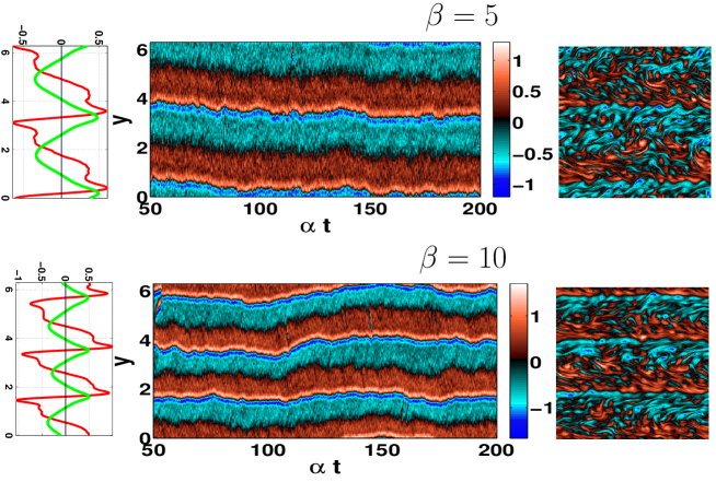
Figure 2: Jets sampled in direct numerical simulations. Left panels show local time averages of the zonally averaged vorticity (red curve) and velocity (green curve) as a function of latitude $y$ ($y$ is the vertical axis), for $\alpha=1.2\cdot 10^{-3}$. Middle panels show the corresponding Hovmöller diagrams of the vorticity $\omega$ (the color represent the value of the zonally averaged vorticity as a function of time and latitude). Right panels show one of the corresponding instantaneous snapshots of the vorticity field. The first line shows these figures at $\beta=5$, the second line shows these figures at $\beta=10$.

In the following, we will be interested in this strong jet regime, which is relevant for Jupiter. Except if otherwise stated, all the computations of this paper will be performed with the parameters $\alpha=1.20\ 10^{-3}$, $\nu=1.5\ 10^{-8}$, and using a stochastic force with a uniform spectrum in the wave number band $|k|\in[14,15]$. The related forcing scale will be always well below the Rhines scale. Figure 2 illustrates that although the flow is clearly turbulent, in the statistically stationary state the zonal jets are very stable on timescale of the order of $10^{5}$ turnover time or more. If $\alpha$ would be decreased, these jets would become even more stable. The averaged vorticity has a saw-tooth profile: it is composed of homogenized potential vorticity areas where the potential vorticity $\omega+\beta y$ is nearly constant (and for which the vorticity decreases approximately like $-\beta y$ across the basin), separated by small areas of abrupt increase of the vorticity (or potential vorticity). This PV staircase phenomenology has been first described by Marcus and Lee (1998) and is only approximately valid (Danilov and Gurarie, 2004). We illustrate in Fig. 3 how the typical potential vorticity mean profile behaves, using the same solution than in Fig. 2.

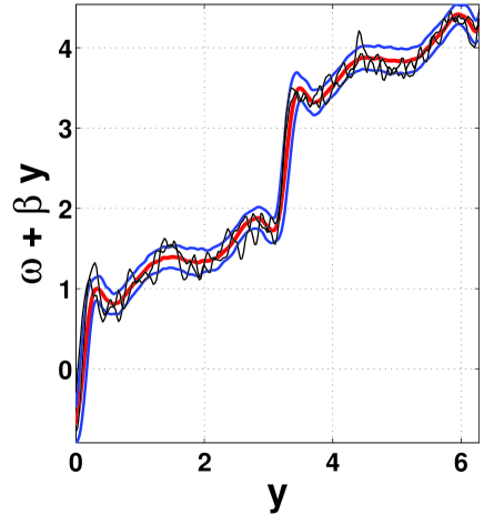
Figure 3: Behavior of the zonally-averaged potential vorticity $\omega+\beta y$ with the same parameters than in Fig.2 ($\beta=5$). The red curve corresponds to the time mean value for $\alpha t\in[100,150]$, the blue curves to the corresponding $\pm$ standard deviations, and the black curves to two different times chosen arbitrarily.

For the velocity profile, homogenized potential vorticity areas correspond to westward jets, with a local quadratic velocity profile with a curvature approximately equal to $\beta$, while the jumps in vorticity give rise to cusps for the velocity close to eastward jets. This phenomenology has been observed in many simulations for barotropic flows. The top panels of Fig. 2 show a state with two alternating jets. There are actually four jets: two eastward jets with local maxima of the zonally averaged velocity and two westward jets with local minima of the zonally averaged velocity. We stress also that, on the Hovmöller diagram, the jet extrema are located on the black area (close to zero vorticity lines). The eastward jets are the black areas with negative (blue) vorticity on the south and positive (red) vorticity on the north. Related to the PV staircase phenomenology, the black areas for eastward jets are very thin line, while the black areas for westward jets have a broader extent. In the doubly-periodic domain of this study, the number of eastward jets has to be equal to the number of westward jets, and jets will come by pairs. We will call a state with $K$ alternating jets, a $K$-jet state, i.e. a state with $K$ eastward and $K$ westward jets.

3 Rare transitions between states with different jet numbers

3.1 Bistability, rare-transitions and hysteresis between states with two and three alternating jets

As stressed in Dritschel and McIntyre (2008), assuming the PV staircase phenomenology with a westward jet curvature of order $\beta$ is sufficient to roughly determine the number of jets: its order of magnitude is then given by the ratio of the domain size divided by the Rhine scale, or equivalently in our non-dimensional units $\sqrt{\beta}$. Figure 2 indeed shows that increasing $\beta$ increases the number of jets.

Compatible with this phenomenology, one expects to see transitions from $K$ alternating jets to a state with $K+1$ ones when $\beta$ is increased. As there is no symmetry breaking in this process, one may expect these transitions to be first-order ones with discontinuous jumps of some order parameters. In situations with discontinuous transitions when an external parameter $\beta$ is changed, one expects for each bifurcation multistability ranges $(\beta_{1},\beta_{2})$ in which two (or more) possible states are observed depending on the initial conditions, and for which extremely rare transition from one state to another may occur due to either external or internal fluctuations. Such a bistability phenomenology has first been observed in Bouchet and Simonnet (2009). The aim of this paper is to go much further in the study of the structure of the attractors and the description of the spontaneous transitions between them.

Figure 4 shows that the bistability occurs for fixed values of the control parameters and a very wide range of initial conditions. We compute the Fourier components of the vorticity, with zonal wave number $(0,n)$, defined as $q_{n}=\frac{1}{|\Omega|}\int_{\Omega}\omega(x,y)\leavevmode\nobreak\ {\rm e}^{iny}dx\leavevmode\nobreak\ dy$, for $n=2$ and $n=3$. Their moduli $|q_{n}|$ are relevant order-parameter, for instance $|q_{2}|$ will be large for a two-alternating jet state and small otherwise. In Fig. 4, one observes five spontaneous $2\to 3$ transitions and five $3\to 2$ transitions for a duration of about $10^{6}$ turnover times. The fluctuations of the three alternating jet states are noticeably larger than the ones for the two alternating jet states. This corresponds to some internal dynamics between several three alternating jet states, as will be explained in section 4.

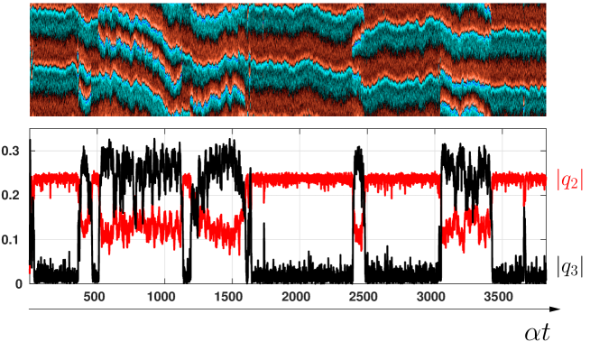
Figure 4: Lower panel: timeseries the moduli of the first zonal Fourier components ($|q_{n}|$ with $q_{n}=\frac{1}{|\Omega|}\int_{\Omega}\omega(x,y)\leavevmode\nobreak\ {\rm e}^{iny}\ {\rm d}x{\rm d}y$) for $n=2$ (red) and $n=3$ (black). The corresponding Hovmöller diagram for the zonally averaged vorticity is shown in the upper panel ($\alpha=1.2\cdot 10^{-3}$ and $\beta=5.2$).

We finally perform an hysteresis experiment by varying adiabatically (very slowly) the parameter $\beta$ at rate $\dot{\beta}=\frac{\alpha}{100}$, in the range $\beta\in[4,12]$, with a smaller value of $\alpha=5\cdot 10^{-4}$. Fig. 5 shows different numerical experiments with independent realizations of the noise. This figure displays the modulus of $|q_{2}|$ as a function of $\beta$ in three of these experiments: the upper branch of $|q_{2}|$ corresponds to the two alternating jet state and the lower branch to the three alternating jet state. It shows bistability in the range $\beta\in[6,11]$, with transitions occurring after a transition time $T\lesssim 10^{5}$: with this slowly varying $\beta$, transition events are not uncommon. However, performing direct numerical simulations for this value of $\alpha$ will not show transitions. The reason is simply that, as explained in the next sections, the probability of seeing such transitions becomes then much too small. Based on the hysteresis curve, we choose $\beta=8$ as a reference value for future studies, unless otherwise specified.

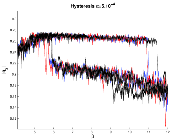
Figure 5: We performed four independent hysteresis experiments, by increasing and then decreasing slowly the value of $\beta$. For the four experiments, each of the four curves represents $|q_{2}|$, the modulus of zonal Fourier component with wavenumber two, as a function of $\beta$ ($\alpha=5\cdot 10^{-4}$ and $\dot{\beta}=\alpha/100$).

3.2 Nucleation and coalescence of jets

We discuss now the spontaneous $2\to 3$ and $3\to 2$ transitions, as seen in Fig.4. While we could not obtain many transitions with direct numerical simulations, using the rare event AMS algorithm, we were able to collect several thousands of $2\to 3\to 2$ transitions. The dynamics of those transitions are represented in Fig.6, in the space spanned by the order parameters $|q_{2}|,|q_{3}|$ and $|q_{4}|$. The remarkable result is that these trajectories seem to concentrate in the phase space. The blue tube in Fig.4 contains 80% of the $2\to 3$ transitions whereas the red tube contains 80% of the $3\to 2$ transitions. The concentration of trajectories that lead to a rare events close a predictable path, is called an instanton phenomenology (see for instance (Laurie and Bouchet, 2015; Grafke et al., 2015; Bouchet et al., 2014; Dematteis et al., 2019) for turbulent flows). Figure 6 illustrates this remarkable instanton phenomenology for the $2\to 3\to 2$ transitions. For this parameter regime, $2\to 3$ and $3\to 2$ transitions occur with a return time approximatively equal to $10^{8}$. Note that it is a very rough estimate based on a single AMS realization. We did not search for more precise estimates here, as we are interested mostly on transitions dynamics. In principle, one should use more realizations with different reaction coordinates (see Appendix B).

The middle-left panel of Fig.6 shows that the nucleation of a new pair of alternating jets proceeds through an inversion of the velocity curvature of one of the parabolic westward jet in the exact middle between the two adjacent eastward jets. It takes the form of a small bump in the zonal velocity profile. This structure indeed nucleates from two bands of positive and negative vorticity inside a narrow band of zero vorticity around the westward jet. Such a nucleation is highly improbable, as the new vortex bands are initially too narrow to be stable. Then just by chance, one can have this band surviving long enough to grow until it reaches a stable state. However, once a critical size is reached, the band becomes stable and grows in size. The three jets slowly equilibrate and separate apart. The new jet can relax either to the north or to the south of the initial parabolic jet where it has nucleated. We will describe this in more details in the next section. In the following, we will call a transition $2\to 3$, a nucleation.

The lower-right panel of Fig.6 shows how two jets can merge, which can be interpreted as the disappearance of one pair of alternating jets. The phenomenology is again rather simple. Interestingly, if one reverses both the time and the sign of the velocity, one would indeed obtain a nucleation from a cuspy (westward) jet. Moreover, the resulting two alternating jet state just after the two eastward jets have merged, is slightly asymmetric (see zonally averaged zonal velocity for the $3\to 2$ transition in Fig.6 and section 4 hereafter). This state then relaxes to a perfectly symmetric two-jet configuration over a timescale of order $1/\alpha$ (not shown). We call the jet merging $3\to 2$ transition a coalescence.

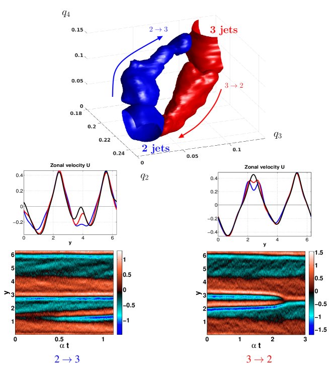
Figure 6: The upper panel shows the level set of the reactive trajectories in the space $|q_{2}|,|q_{3}|,|q_{4}|$. The blue and red reactive tubes contain 80% of the $2\to 3$ transitions and $3\to 2$ transitions, respectively. Each of these tubes gather about $1000$ reactive trajectories obtained using the AMS algorithm, for $\alpha=10^{-3}$ and $\beta=8$. Middle left and right panels show the zonally averaged zonal velocity as a function of latitude, 3 curves at 3 different times (blue first, then red, then black), during the $2\to 3$ and $3\to 2$ transitions, respectively. On the left, we observe the nucleation of a new jet at the westward tip of an existing jet. On the right, we observe the merging of two eastward jets. Lower left and right panels are the two corresponding Hovmöller diagrams for the zonally averaged vorticity.

3.3 Barotropic adjustment and Rayleigh-Kuo criterion for zonal jets and during transitions

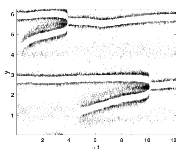
Figure 7: The Rayleigh–Kuo criterion for an example with two nucleations and two mergers. This is a Hovmöller diagram where black dots are plotted each time $RK=U^{\prime\prime}-\beta$ is positive ($\alpha=2.2\ 10^{-4}$ and $\beta=5.5$).

Are rare transitions between attractors driven by hydrodynamic instabilities? This is a very natural fluid mechanics question that we address now. It is clear from all the Hovmöller diagrams, on Figs 2 and 6 and on movies of the dynamics (not shown), that the time scale for the transition dynamics is of order $1/\alpha$, both during a nucleation of new jets or during a coalescence. This is also true for all other transitions we have observed. This phenomenology thus excludes a fast instability in the barotropic equation (2), developing on time scales of order one. As a consequence, if some instability occurs in equation (2), the flow has to be marginally unstable with an instability rate scaling at most like $\alpha$ when $\alpha\downarrow 0$.

Such an observation of marginal instability is related to the classical hypothesis of barotropic adjustment of eddy-driven jets (see Read et al. (2020b, a) and references therein). An eddy-driven jet with a time-scale separation between eddy dynamics and zonal jet time scale, should be unstable in order to transfer meridionally zonally-averaged momentum, while it should be at the same time stable if quasi-stationary zonal jet states are observed for very long times. This apparent contradiction leads to the hypothesis of barotropic adjustment: the state of the system should be marginally stable (or unstable) in order to fulfill these two seemingly contradictory requirements. The relevance of this adjustment hypothesis has been recently discussed in the context of Jovian planets and for a hierarchy of models (Read et al., 2020b, a). The interesting remark we want to stress here is that this barotropic adjustment mechanism actually takes place for the statistically quasi-stationary jets, as might be expected, but perhaps more unexpectedly, also takes place during the periods of relaxation towards these quasi-stationary states and during the periods of ”instability” that lead to coalescences and nucleations of jets.

In order to have a more precise and quantitative insight on this issue, we look at the Rayleigh–Kuo criterion $RK=U^{\prime\prime}-\beta$, where $U^{\prime\prime}$ is the second derivative with respect to $y$ of the zonally averaged zonal velocity $U$. It is well known that, for a zonal flow $U(y)$, a necessary condition for an hydrodynamic instability to occur is that the Rayleigh–Kuo criterion changes sign (H.L.Kuo, 1949). Figure 7 is a Hovmöller diagram of the sign of the Rayleigh–Kuo criterion: we draw a black point each time the Rayleigh criterion is negative. This picture is drawn from an example of a $2\to 3$ transition obtained with the adaptive multilevel splitting algorithm ($0<\alpha t<1.3$) followed by a free dynamics (Eq. (2) without selection) ($1.3<\alpha t<12$), with the parameters $\alpha=2.2\ 10^{-4}$ and $\beta=5.5$. The eastward jets are localized inside the thin white bands delimited by the area with dense black dots. The westward jets are localized in the area with lots of scattered black dots, but with a much lower density than at the flank of eastward jets. The picture then shows subsequently: a nucleation of new jets at the location of a westward jet ($0<\alpha t<1.3$), the northward drift of one of these new jets until it reaches another eastward jet and coalesces ($1.3<\alpha t<4$), a transient state with two alternating jets ($4<\alpha t<4.9$), the nucleation of new jet and the drift northward of one of them, until a new coalescence ($4.9<\alpha t<10.2$), and a stable state with two alternating jets ($10.5<\alpha t<12$).

We first describe in detail Fig.7 during the period with a stable state with two alternating jets ($10.5<\alpha t<12$). We note that most of the time, the Rayleigh-Kuo criterion is positive, meaning that the overall structure is stable. However, from time to time, the Rayleigh–Kuo criterion changes sign on some specific points of the domain. During that period, the velocity profile $U$ looks very much like the one of the two-jet state. On this curve, we see a characteristic shape for eastward jet velocity profile, with a characteristic cusp shape. At the edge of the eastward jet, the cusp is associated with a very strong negative curvature and thus a very low value of $RK=U^{\prime\prime}-\beta$, explaining the white band without black dots on Fig.7. On each flank of the jet, the velocity profile has a concavity change, where $RK$ changes sign very often, explaining the two dense black dot bands surrounding the eastward jet. On all the other parts of the flow, $RK$ remains much of the time positive, except close to the westward jet, where $U^{\prime\prime}$ is very close to $\beta$ and $RK$ changes sign rather often. This explains the less dense band of black dots close to the westward jet edge. We stress also that the shape of eastward jet cusps seems to depend significantly on the dissipative mechanism. Indeed, Figs 2 and 6 show that, for larger values of $\alpha$ for which hyperviscosity effects are negligible, the cusp is rather rounded, while other simulations with smaller values of $\alpha$ (not shown), for which hyperviscosity effects become important, the velocity profile has a strong concavity change on the flank of the jet. In a recent theoretical work (Woillez and Bouchet, 2019), it has been established that: i) eastward jets should form a cusp, with a width of order $1/K$ where $K$ is the typical random force wavenumber, and which specific profile depends on the dissipative mechanism, ii) the mechanism preventing the growth of westward jet is a marginal instability of the velocity profile appearing when the positive curvature of the jet is of order $\beta$. Our numerical observations are thus in line with this theoretical work.

Using Fig.7, we now describe the jet nucleations and coalescences, from the point of view of the Rayleigh–Kuo criterion. First we observe that during the nucleation processes, we do not see any change of sign for the Rayleigh–Kuo criterion that would qualitatively differs from the stable jet situation. Second, during the coalescence, a black band appears at the level of the westward jet squeezed between two eastward jets, just before the coalescence. In this area, although we cannot conclude from this figure, the Rayleigh–Kuo criterion may change sign. As the Rayleigh–Kuo criterion is only a necessary condition for instability, we can not conclude from this figure if a very localized and very low rate instability may occur during the coalescence. However, if such an instability actually occurs, its rate has to be very small, as the typical time scale for the change of the structure is very long, of order $1/\alpha$.

We conclude that the flow is constantly marginally stable close to westward jets, in accordance with a barotropic adjustment picture. This is the case for stationary states, as we already analyzed and discussed theoretically in Woillez and Bouchet (2019), but this is also the case during both the coalescence and the nucleation transitions. This marginal stability is thus not specifically related to transition trajectories, as it also occurs for stationary states. We conclude that this marginal stability (or instability) is not by itself the driver of the transitions.

In this section, we have addressed the hydrodynamical stability of the flow. We have seen that no hydrodynamical unstability occurs, although marginal stability is always present. A different question is wether the slow effective dynamics that describes the flow on longer time scale should be unstable or not. It should be unstable, at some point, because of the observed saddle point phenomenology. When transitions occur, in order to pass the saddle point, the noise has to compensate the instability of the slow effective dynamics. On the slow timescale, the relevant noise is the one produced by the fluctuations of the divergence of the time average of the Reynolds stress. We discuss this in the next section.

3.4 Saddle points

In the following, we will use the language of dynamical system theory plus weak noise, in order to describe the phenomenology of the attracting states and the transition dynamics between them. This dynamical system discussion applies to the slow effective dynamics of the zonally averaged zonal velocity $U(y,t)=\frac{1}{2\pi}\int_{0}^{2\pi}u(x,y,t)\leavevmode\nobreak\ dx$. Indeed, in the regime of small values of $\alpha$, as argued in Bouchet et al. (2013), we expect the slow relaxation dynamics of zonal jets to be described by a deterministic effective equation that can be obtained through a second cumulant closure. This kinetic theory has been extended to take into account marginally stable modes (Woillez and Bouchet (2019)) as it occurs at the tip of westward jets (see previous sections).

Besides such deterministic effective equations, the transitions from one attractor to another are expected to be triggered by a noise, due to the fluctuations of the Reynolds stress divergence, which properties can be computed using large deviation theory as explained in Bouchet et al. (2018). Based on these theoretical works, we expect the effective dynamics to follow.

$$\partial_{\tau}U=F(U)+\sqrt{\alpha}\sigma(U,\tau),$$ (3)

with the rescaled time $\tau=\alpha t$, the average of the divergence of the Reynolds stress divergence $F(U)$, and a white noise $\sigma(U,\tau)$ related to the fluctuations of time average of the divergence of the Reynolds stress.

Interesting formulas for $F$, implying local derivatives, were proposed by Srinivasan and Young (2014), or by Laurie et al. (2014) in a different but related context. As explained in Woillez and Bouchet (2019), such local formulas and others can be justified in the limit when the forcing scale is much smaller than the jet width, and lead to interesting dynamical consequences. However this is only valid in flow areas with strong enough shear. Such local formulas would thus not be valid globally for the flow, for instance close to jet tips, even if the spatial scale separation would be present. We conclude that, while the theoretical works clearly justify the existence of equation (3) under some natural hypothesis, the formulas for $F$ and $\sigma$ are not explicit in general. They might be computed numerically. In the absence of analytical expression and easy numerical computation from the theory, the aim of this work is to directly verify the dynamical and qualitative consequences of (3) without computing explicitly $F$ and $\sigma$.

The attractors and saddle points should be thought as attractors and saddle points of the deterministic dynamics $\partial_{\tau}U=F(U)$. Although there is no explicit knowledge of $F$, such attractors and saddle points can neverveless be directly observed in fully turbulent direct numerical simulations, or in fully turbulent simulations using the AMS algorithm. In a fully turbulent simulation, a saddle point belongs to a transition trajectory. Moreover, when adding small perturbations it can either relax to one attractor or to the other depending on the perturbation. Those two properties are enough to characterize them numerically, as we better explain in appendix B.c.

For the value $\beta=8$, the hysteresis curve in Fig.5 suggests that the system is multistable with at least two attractors. For dynamical systems with weak noise, in the simplest cases, the transitions from one attractor to another must go through a saddle point which belongs to the common boundary of the two basins of attraction. In more complex situations, the transitions could rather proceed through more complex structures, for instance saddle limit cycles or saddle strange attractors. These scenarii where two basins collide are called crisis bifurcations (Grebogi et al., 1983). As we describe in the following, we have detected saddles points only for the dynamics of the $2\to 3$ and $3\to 2$ transitions.

Using AMS results, we are able to easily find these saddle states, using the methodology described in appendix B.c. They are shown in Fig.8 for the nucleation. As mentioned before, the new jet is created from the parabolic jet at the middle of the two westward jet. This new jet can drift either to the north or to the south. This is illustrated by the presence of two different ensembles in the AMS reactive trajectories giving two different saddles. The difference is small however and it is possible that in other parameter regimes, these two saddles collapse into a single one at the exact middle of the two westward jets. This is discussed in the next sections. Note that, in addition, one must add two other saddles related to the nucleation at the other westward jets. Moreover, it is possible that one observes direct transitions $2\to 4$ involving four possible double nucleations (north north, north south, south north and south south). We have indeed observed such transitions (not shown), but we have decided not to discuss higher-order transitions involving several transitions at the same time, that is transitions of codimension larger than one.

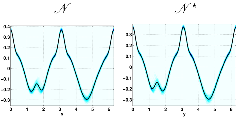
Figure 8: Zonally averaged velocity as a function of latitude, $U(y)$, for the nucleation saddles. Each black curve is obtained by the ensemble average of the output of about 800 AMS runs ($\alpha=10^{-3}$ and $\beta=8$). Please note the slight asymmetry of each of the saddles, close to the westward tip of the nucleating jet. For each value of $y$, we have superimposed the histograms of the $U$ values of the 800 AMS states (light blue), in order to feature the spread of the ensemble values.

A similar study of the saddle points for the transitions $3\to 2$ is discussed in Fig.9. If the distance between the two closest jets is below a certain critical distance (approximately one sixth of the domain width), they start to be attracted to each other until they merge into a single jet. On the contrary, if their distance is above this critical value, the whole system relaxes to a stationary three-jet state. This critical distance appears to be rather sensitive to the value of $\beta$. This distance increases as $\beta$ decreases and decreases for larger values of $\beta$. This is consistent with the idea that for a regime where only the two-jet states dominate, say for smaller values of $\beta$, the three-jet states will be easily destabilized though the coalescence process. One may ask, why only one saddle is found ? The reason is simply related to the initial conditions used in the AMS. In fact, there are as many coalescence saddles as nucleation saddles. This point is clarified in section 4.

Two natural scenario can be considered for the transitions between states with various number of jets either: i) an hydrodynamic instability of the base flow $U$ or ii) instabilities in the effective dynamics that describe the evolution of the flow on longer time scales after averaging. Constantinou et al. (2014) shows clear evidence of scenario ii) for some range of parameters. From the discussion in this section and the previous one, we see that the dynamics described in this paper follow a third scenario, with both marginal stability for the hydrodynamic equations and instability of the effective dynamics. Indeed, as explained in the previous section our flow is constantly marginally stable. This marginal stability might or might not be related to the transition dynamics. Then one needs to generalize effective theories in order to describe long term dynamics of the zonal jet in order to take into account marginally stable states, for instance following Woillez and Bouchet (2019). Then, the existence of saddle points requires instabilities of the effective dynamics. Our third scenario has thus flavors of both scenario i) and ii).

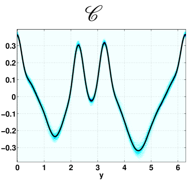
Figure 9: Zonally averaged velocity as a function of latitude, $U(y)$, for the coalescence saddle. Each black curve is obtained by the ensemble average of the output of about 200 AMS runs ($\alpha=10^{-3}$ and $\beta=8$). For each value of $y$, we have superimposed the histograms of the $U$ values of the 800 AMS states (light blue), in order to feature the spread of the ensemble values.

3.5 Instantons

Figure 6 strongly suggests the existence of an instanton-driven dynamics. By this, we mean that jet nucleation or coalescence events are concentrated around a predictable path, called instanton. These paths are composed of a rare noise-driven fluctuation path from the two alternating jet attractors toward a saddle point (for instance), then of a typical relaxation path from the saddle point to the three alternating jet attractor. If our hypothesis is correct, as $\alpha\to 0$ the reactive tubes shown in Fig. 6 should collapse to a single instanton path (see Appendix A). By an abuse of language, we will assume that this is the case and we identify the instanton with the reactive tube. This is justified and discussed in section 5, when we vary $\alpha$.

The important point is that two different saddles are involved in the $2\to 3$ and $3\to 2$ transitions, and not just one. The consequence is a more subtle structure which is not seen in the two crude Fig.6. This is explained by the schematics of Fig.10. Let us denote the two alternating jet attractor and the three alternating jet attractor $J_{2}$ and $J_{3}$ respectively. In Fig.10, the nucleation instanton is the red curve starting from $J_{2}$ and going to ${\cal N}$ together with its relaxation part (black curve) from ${\cal N}$ to $J_{3}$. Similarly, the coalescence instanton is the red curve starting from $J_{3}$ to ${\cal C}$ and its relaxation part (black curve) goes from ${\cal C}$ to $J_{2}$. The relaxation curves (black curves) correspond to trajectories having zero action in the asymptotic limit since they correspond to the natural dynamics of the system. Figure 8 shows that the left schematic of Fig.10 has moreover a mirror equivalent shown to the right. The mirror states are denoted here with a star for convenience.

Moreover, to each instanton is associated an anti-instanton going through the same saddle. The pair instanton anti-instanton forms a so-called figure-eight pattern in phase space.

The time asymmetry does not only translate into a geometrical asymmetry of the pair instanton anti-instanton, but the transition probability of corresponding reactive trajectories is different as well. It appears that in this model, the asymmetry is very strong especially in terms of transition probabilities: the “anti-transition” probabilities are several order of magnitude smaller than the transition probabilities. For instance, the ”anti-coalescence” instanton corresponds to a path going from $J_{2}$ to ${\cal C}$ (thin red curve) and then from ${\cal C}$ to $J_{3}$ (relaxation black curve). It requires an inversion of the curvature on the top of one of the eastern cuspy jets followed by a separation of the two small jets which are created off the cusp. Such events are of course very rare but can be detected by AMS. The probability of an inversion of the cusp curvature is estimated by AMS to be $O(10^{-9})$. However, the nucleation of an eastward jet leading to the configuration shown in Fig. 9 has a considerably smaller probability, estimated by AMS to be less than $O(10^{-30})$.

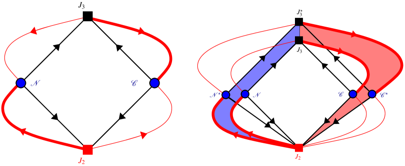
Figure 10: Schematic representation of the instantons involved in the transitions $2\to 3\to 2$. Left figure is a simplification of the right figure, ie without representing the dual mirror pair of states. $J_{2}$ is the stationary two-jet state, $J_{3}$ and $J_{3}^{\star}$ are the two mirror-symmetric three-jet states obtained from the two nucleation saddles called ${\cal N}$ and ${\cal N}^{\star}$ (see Fig.8). The coalescence saddles are called ${\cal C}$ and ${\cal C}^{\star}$ (see Fig.9). The black arrows represent the relaxation trajectories from the saddle to the attractors (with zero action; see Appendix A). The red curves correspond to the reactive part of the instantons (with nonzero action). The colored area inside the bold curves is what is shown in instanton tubes of Fig.6, that is half of the actual instanton structure.

We describe in the next section the internal effective dynamics of the state with three alternating jets.

4 States with three alternating jets and their internal dynamics

The previous results indicate the existence of at least two types of states having three alternating jets, due to different possible nucleations (see Fig.8) or coalescences (see Fig.9). It was previously referred to as a mirror symmetry without being too precise on what symmetry was involved. We show next that the reality is more complicated, with the description of several different states with three alternating jets, and a slow dynamics between them. This explains in particular the large amplitude of the fluctuations of the three alternating jet states, as seen in Fig.4.

4.1 New representation of the jet attractors and their dynamics

In order to describe this structure, we need a more precise description of the jet profiles (the zonally averaged zonal velocity). If one measures precisely the distance between the jet tips, one observes some slight asymmetries in the three alternating jet states. Indeed, the attractors do not equilibrate to an equidistant jet solution, see for instance the three alternating jet states in Fig.4. This asymmetry is robust when $\beta$ is changed. Based on this remark, it is relevant to characterize these states by the distance between the eastward jet tips for instance. These distances give three numbers we call $\sigma_{1},\sigma_{2},\sigma_{3}$. Our convention is to divide these quantities by the dimensionless domain width $2\pi$ so that $0\leq\sigma_{i}\leq 1$. Due to the periodicity in $y$, one has the constraint

$$\sigma_{1}+\sigma_{2}+\sigma_{3}=1.$$

Given this constraint, in the following, we prefer to consider the most economical representation and use only two of these quantities, say $\sigma_{1}$ and $\sigma_{2}$. Looking at the Hovmöller diagram of Figure 4 for instance, one observes some slow drift of the solution in the meridional direction. We therefore choose one of the eastern jet as a reference moving frame, and compute $\sigma_{1}$ and $\sigma_{2}$ from this reference jet. $\sigma_{1}$ is the distance between this reference jet and the next eastward-jet tip, northward. $\sigma_{2}$ is the distance between this new jet and the next eastward-jet tip, northward again. This procedure is for measurements only and requires to always track the same reference jet at any time. A state with three alternating jets will be thus described by $(\sigma_{1},\sigma_{2},\sigma_{3}=1-\sigma_{1}-\sigma_{2})$.

The values taken by $\sigma_{1}$, $\sigma_{2}$ and $\sigma_{3}$ are always very close to three fixed values $\sigma_{1}^{*}$, $\sigma_{2}^{*}$ and $\sigma_{3}^{*}$ which are all different from $1/3$ and different from each others. On figures 12, 13 and 14 one sees that $(\sigma_{1}^{*},\sigma_{2}^{*},\sigma_{3}^{*})\simeq(0.23,0.34,0.43)$ with fluctuations with standard deviations of order $0.013$. For a given configuration $(\sigma_{1}^{*},\sigma_{2}^{*},\sigma_{3}^{*})$ there are two other symmetric configurations by meridional translation: $(\sigma_{2}^{*},\sigma_{3}^{*},\sigma_{1}^{*})$ and $(\sigma_{3}^{*},\sigma_{1}^{*},\sigma_{2}^{*})$. However there exists also three other states that can not be recovered by meridional translation from the first one $(\sigma_{2}^{*},\sigma_{1}^{*},\sigma_{3}^{*})$, $(\sigma_{3}^{*},\sigma_{2}^{*},\sigma_{1}^{*})$ and $(\sigma_{1}^{*},\sigma_{3}^{*},\sigma_{2}^{*})$, but can be recovered if we use a mirror symmetry. These 6 states are in correspondence with all the permutations of $\{1,2,3\}$, three even permutations and three odd permutations.

For clarity, Fig.11 shows a schematic of these configurations. The group of permutation is called ${\cal S}_{3}$ and possesses $3!=6$ possible permutations: $\{123,231,312,213,321,132\}$.

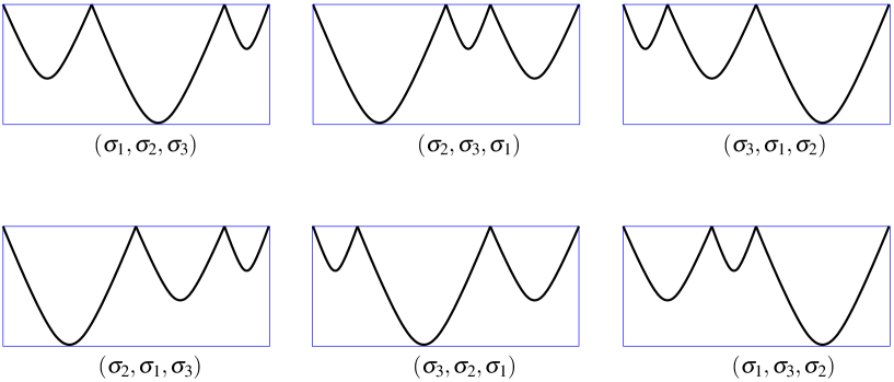
Figure 11: Sketch of the zonal velocity as a function of latitude, $U(y)$, generated by the symmetry group for the six different configurations, with three-alternating jet. We have amplified the meridional asymmetry of the jets for better visualisation.

We now show in the next subsections a remarkable result: the symmetric group ${\cal S}_{3}$ is indeed realized by the natural dynamics of the system.

4.2 Probability density in the $(\sigma_{1},\sigma_{2})$ plane

We perform a direct numerical simulation with some long time integration of equation (2), and we measure the distances $\sigma_{1}$ and $\sigma_{2}$. This probability density function of $(\sigma_{1},\sigma_{2})$ is shown in Fig. 12. The time averaged values obtained from this dataset gives $\langle\sigma_{1}\rangle=\sigma_{1}^{*}\approx 0.340$ and $\langle\sigma_{2}\rangle=\sigma_{2}^{*}\approx 0.226$ with fluctuations for $\sigma_{1}$ and $\sigma_{2}$ being of the same order, of about $\pm 0.013$.

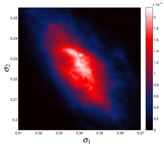
Figure 12: Probability density function of $(\sigma_{1},\sigma_{2})$ for one of the states with three alternating jets ($\alpha=10^{-3}$ and $\beta=8$).

Figure 13 shows that when one integrates the system over a very long period of time, metastability is indeed observed between the six states. We denote $\langle\sigma_{1}\rangle$ the value of $\sigma_{1}$ averaged over a sliding time windows over a small enough period of time. It reaches three distinct values $\langle\sigma_{1}\rangle\in\{0.23,0.34,0.43\}$ corresponding to the three values $\{\sigma_{1}^{*},\sigma_{2}^{*},\sigma_{3}^{*}\}$. A closer inspection of the quantities $\sigma_{1}$, $\sigma_{2}$, shows that the system is indeed wandering around four distinct configurations denoted $a,b,c,d$ in Fig.13. When one integrates for a sufficiently long period of time, the number of possible configurations is in fact 6, in correspondance with the 3! permutations of the symmetric group ${\cal S}_{3}$.

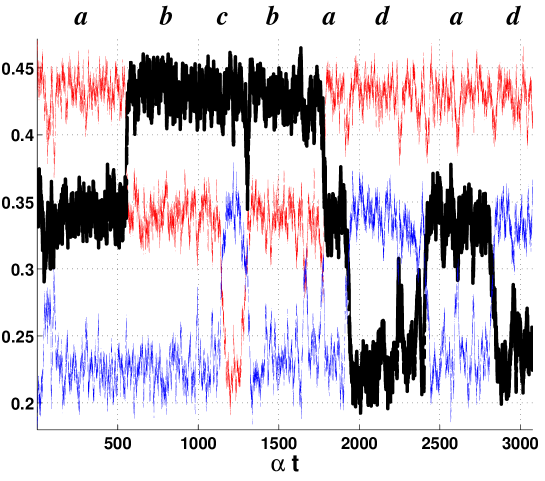
Figure 13: Timeseries of $\sigma_{1}$ (black curve) together with $\sigma_{2}$ (blue curve) and $\sigma_{3}$ (red curve) with the time axis rescaled by $\alpha=10^{-3}$.

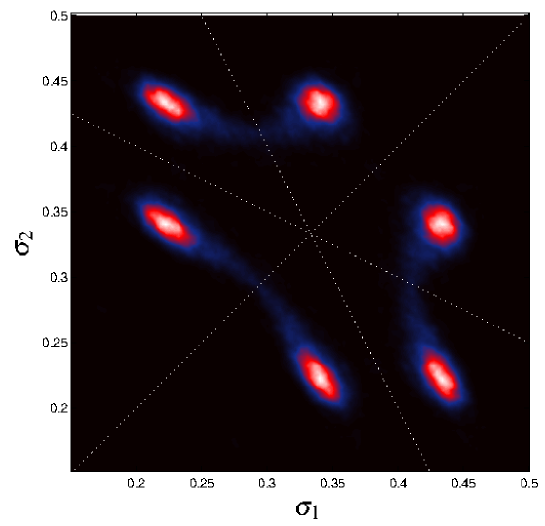
Figure 14: Probability density of $(\sigma_{1},\sigma_{2})$ featuring the six different states with three alternating jets. The three dotted lines correspond to states with two equally distant jets, they intersect at $(\sigma_{1},\sigma_{2},\sigma_{3})=(\frac{1}{3},\frac{1}{3},\frac{1}{3})$. Figure 12 is a zoom of the states in the lower-left sector corresponding to configuration $a$. The blue traces inbetween the states feature reactive trajectories statistics.

The probability density function of the full set is shown in Fig.14. One clearly sees in light blue some traces of transitions between pairs of adjacent states. As explained in the next subsection, all states are indeed connected by two type of transitions, one toward each adjacent state.

4.3 Internal saddles

The transitions observed must involve saddles with two equally distant jets and are therefore located on the white dot lines of Fig.14. Let a state be written as $(\sigma_{1},\sigma_{2},\sigma_{3})$ and let $i,j,k\in\{1,2,3\}$ such that $\sigma_{i}<\sigma_{j}<\sigma_{k}$. Then type-I transitions correspond to transitions where the two smallest distances have been switched so that the new state has $\sigma_{j}<\sigma_{i}<\sigma_{k}$. Indeed, it can be seen in Fig.14 by looking at the visible blue traces. This is a consequence of the two possible nucleations of the form $(\frac{1}{4}-\epsilon,\frac{1}{4}+\epsilon,\frac{1}{2})$ and $(\frac{1}{4}+\epsilon,\frac{1}{4}-\epsilon,\frac{1}{2})$. Type-II transitions follow the same type of rule, where instead, the two largest distances are involved. In the example above, the new state will be such that $\sigma_{i}<\sigma_{k}<\sigma_{j}$. It is clear that there are no possible transitions where the smallest and largest distances are switched, as it would require to go through the perfectly symmetric state $(\frac{1}{3},\frac{1}{3},\frac{1}{3})$: the system prefers to visit two configurations before, through one type-I transition, and one type-II transition. By symmetry, we conclude that there are a total of three type-I saddles and three type-II saddles. Those saddles are computed as discussed in Appendix B.c. Type-I saddles have two equally-small distances and are shown in Fig.15. Type-II saddles have two equally-large distances and are shown in Fig.16.

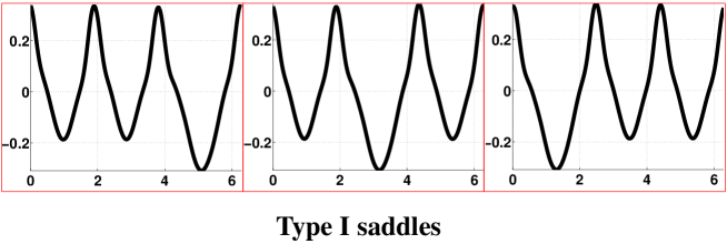
Figure 15: The three type-I saddles $(\sigma,\sigma,1-2\sigma),(\sigma,1-2\sigma,\sigma)$ and $(1-2\sigma,\sigma,\sigma)$ are located at the intersections between the dot lines and the blue traces of Fig.14 with $\sigma\approx 0.30$. The corresponding zonally averaged zonal velocities as a function of latitude, $U(y)$, which were obtained by direct numerical simulation, are represented.

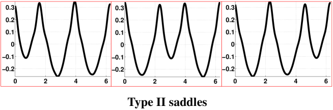
Figure 16: The three plots show the zonally averaged zonal velocities as a function of latitude, $U(y)$, for the three type-II saddles $(\sigma,\sigma,1-2\sigma),(\sigma,1-2\sigma,\sigma)$ and $(1-2\sigma,\sigma,\sigma)$ with $\sigma\approx 0.37$. They have been obtained by direct numerical simulations.

4.4 Effective dynamics: summary

We first mention that one can represent a two-jet state in our $(\sigma_{1},\sigma_{2})$ parameter plane in different ways as there is one missing jet. We decide to choose the one which is consistent with the dynamics in the limit where one jet appears or disappears. One must identify first the four corners $(0,0)\equiv(0,\frac{1}{2})\equiv(\frac{1}{2},0)\equiv(\frac{1}{2},\frac{1}{2})$ as a single state. During the nucleation process, the initial perturbation before reaching the nucleation saddle is a jet of the form $(\frac{1}{4},\frac{1}{4},\frac{1}{2})$ (plus permutations) and the nucleation saddle is of the form $(\frac{1}{4}+\epsilon,\frac{1}{4}-\epsilon,\frac{1}{2})$ and its five symmetric partners making a total of six different nucleation saddles. One can measure the numerical value of $\epsilon$ from Fig.8, it gives $\epsilon\approx 0.01$. The same rule applies for the coalescence saddles, there are a total of six coalescence saddles. Figure 17 is a summary of all the results.

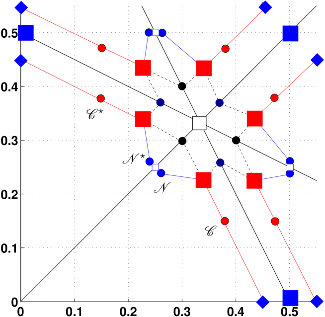
Figure 17: Effective phase space structure in the $(\sigma_{1},\sigma_{2})$ plane, including all ${\cal S}_{3}$ symmetric states. The red squares are the three-alternating jet states, the blue squares correspond to the two alternating jet symmetric states. The blue diamonds are asymmetric two-alternating jet states obtained just after the coalescence process. Red circles are the coalescence saddles, blue circles are the nucleation saddles, black circles are type-I internal saddles and dark blue circles are type-II saddles. The middle square is the (unstable) three alternating jet symmetric state. The states just before the nucleations are shown as small white squares. The positions correspond to observed numerical values. The dot lines are the internal mirror transitions responsible for metastability and the solid blue and red lines are the $2\to 3$ and $3\to 2$ transitions, respectively.

Despite its simplicity, one should remark that there is, in addition, sub-internal low-frequency variability within a single of the six states with three alternating jets as observed in Fig.12. This suggests the existence of additional saddles possibly within the white S shape visible in Fig.12. We do not show the anti-instantons $2\to 3\to 2$ whereas the internal type-I and type-II pairs of instantons anti-instantons obviously coincide. Note also that higher-order transitions do exist and complicate the picture, one can observe for instance examples where nucleations and coalescences are superimposed, associated with transient four-jet states in addition with the double-nucleation scenario. These events occur with a smaller probability and are not studied here.

Our system is in a regime where at least two successive ${\cal S}_{3}$ symmetry-breaking bifurcations of the effective dynamics have occurred, one related to type-I transitions and one to type-II. Due to that, internal and complex low-frequency variability can induce rather large fluctuations of the states with three alternating jets. The scenario is in fact similar to the typical deterministic one, where global bifurcations like homoclinic and heteroclinic bifurcations force the system to have large-amplitude oscillations. One can readily anticipate that there are simpler regimes unfolding from the perfectly symmetric state. Changing $\beta$ does not seem to change radically the internal structures shown in Fig. 17, except for the saddles involved in the transitions $2\to 3\to 2$ which move either to the states with two alternating jets or the states with three alternating jets, depending on how $\beta$ is changed. It is plausible that, changing for instance the aspect ratio of the domain, could reveal situations where the state $(\frac{1}{3},\frac{1}{3},\frac{1}{3})$ is an attractor. We did not explore these interesting possibilities.

5 Large deviations and the Arrhenius law

We now address the important question of the dependency of the attractor structure and the transition rate between attractors, with respect to the parameter $\alpha$. From equation (3), as a direct consequence of Freidlin-Wentzell theory (Freidlin and Wentzell, 1984), a large-deviation principle for the full system can be inferred. The main ideas of Freidlin–Wentzell large deviation theory are sketched in Appendix A.

In particular, an Arrhenius law must be present. If we call $T$ the mean waiting time before a spontaneous transition occurs, an Arrhenius law with large deviation rate $\alpha$ is a relation $T\propto{\rm exp}\left(\frac{\Delta V}{\alpha}\right)$. $\Delta V$ can be computed from $F$ and $\sigma$ in equation (3) by formula (A2) in appendix A. Moreover, as explained in section 33.4, the existence of $F$ and $\sigma$ and their definition from equation (2) are justified in the limit $\alpha\rightarrow 0$, in the theoretical works Bouchet et al. (2013) and Bouchet et al. (2018), respectively. Moreover those works explain how to compute $F$ and $\sigma$ in principle from equation (2). This gives a way to possibly compute $F$, $\sigma$ and $\Delta V$ numerically from (2) and (A2). However, this is a very complex numerical/theoretical program that has not been performed so far. In this section, we will follow another route and check through direct numerical simulations and the AMS algorithm the Arrhenius law.

A consequence of the large-deviation principle is that the effective dynamics described in Fig. 17 is indeed valid in the limit $\alpha\to 0$, so that reactive tubes, such as those shown in Fig. 6, in this case concentrate near well-defined instanton paths.

Table 1: Mean values of $\sigma_{1}^{*}$ and $\sigma_{2}^{*}$ for the jet attractors shown in Fig.12 as a function of $\alpha$.

$\alpha$	$<\sigma_{1}>$	$<\sigma_{2}>$	std
$8\cdot 10^{-4}$	0.342	0.213	$1\cdot 10^{-2}$
$6\cdot 10^{-4}$	0.342	0.202	$8\cdot 10^{-3}$
$4\cdot 10^{-4}$	0.340	0.191	$6\cdot 10^{-3}$
$2\cdot 10^{-4}$	0.334	0.177	$4\cdot 10^{-3}$

We now discuss our last experiment aimed at checking Arrhenius law. Using the AMS algorithm, we compute for different values of $\alpha$, the mean waiting time to observe the $2\to 3$ nucleation transitions. Note that we have used a different value of $\beta=5.5$ instead of $\beta=8$. The dependency on $\beta$ is in fact irrelevant, as the result we discuss here is mostly insensitive to $\beta$. Note also that although the probability of $2\to 3$ transitions actually depends on $\beta$, the nucleation phenomenology remains unchanged. The result is shown in Fig.18 and is consistent with the existence of an Arrhenius law of the form $T\propto{\rm exp}\left(\frac{\Delta V}{\alpha}\right)$. Such an Arrhenius law is a remarkable fact.

If one decreases $\alpha$ even further, the scaling observed in Fig.18 does not correspond anymore to the simple Arrhenius law (not shown). This is most probably because viscosity $\nu$ is not negligible anymore for so small values of $\alpha$. Then, the working hypothesis $\nu\ll\alpha$ in order to obtain $T\propto{\rm exp}\left(\frac{\Delta V}{\alpha}\right)$ is no more valid. To support this hypothesis, one can observe that the mean energy expected to be equal to one for negligible values of $\nu$, drops to values significantly smaller than one when one uses such small values of $\alpha$. Using smaller value of $\nu$ to test further the Arrhenius law would require to make much more costly numerical simulation with a higher resolution, which would be extremely difficult.

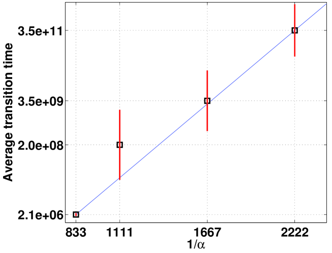
Figure 18: Logarithm of the mean first transition time $T$ as a function of $\frac{1}{\alpha}$ for the $2\to 3$ nucleation transitions. The number of clones for the AMS algorithm is $N=1000$, and two to three independent algorithm realizations were performed. Error bars are a crude approximation of the AMS variance based on the different realizations.

It is important to understand that such scaling law cannot be revealed by direct numerical simulations as illustrated by the table 2: The amount of required CPU time to study the Arrhenius law with a direct numerical simulation increases exponentially as $\alpha$ decreases, whereas using the AMS the required CPU time increases only linearly (see Appendix B).

Table 2: CPU time (d:day,y:year) needed to obtain about $1000$ $2\to 3$ transitions using 200 processors for both AMS and DNS and for different values of $\alpha$.

$\alpha$	AMS	DNS
$1.20\cdot 10^{-3}$	1.0 d	15 d
$0.90\cdot 10^{-3}$	1.4 d	210 d
$0.60\cdot 10^{-3}$	2.2 d	$\sim$ 51 y
$0.45\cdot 10^{-3}$	3.4 d	$\sim$ 2050 y

6 Conclusion

Using the AMS rare event algorithm, we are able to obtain a complete statistical description of the dynamics of planetary jets in a simple barotropic quasigeostrophic model. We show that the spontaneous appearance of new jets come from noise-activated nucleations originating from the westward jets. The disappearance of a jet is in fact the merging between two eastern jets as they become attracted to each other if they are too close. We call this event a coalescence. By collecting thousands of these transitions, we show that they concentrate near some preferred transition paths suggesting the presence of instantons in the limit of vanishing noise. A computation of the mean first-passage time as a function of the Ekman dissipation $\alpha$ reveals a scaling law clearly compatible with an Arrhenius law. This implies that the observed phenomenology is indeed instanton-driven. As a by-product of our rare event algorithm, we are also able to compute the saddles of the effective dynamics.

We next focus on the internal dynamics of solutions having three eastward and westward jets. Surprisingly, it shows a striking example of internal metastability. The state with three alternating jets appears to have jets not at equal distance to each other. We show that there are in fact six distinct configurations which are governed by the symmetric group of permutation called ${\cal S}_{3}$. The consequence is a complex dynamics with low-frequency variability and large fluctuations. This behavior originates from at least two ${\cal S}_{3}$ symmetry-breaking bifurcations of the effective dynamics associated with two different types of transitions depending on the distance between the jets.

We stress that these results are generic. For instance, the observed internal metastability of the three-jet states should appear as soon as there is some asymmetry in the jet positions and shapes. It comes from deeper algebraic constraints linked to the symmetries of the solutions. To this respect, changing $\beta$ should not alter this picture but rather has an impact on the stability of these states. As discussed before, changing $\alpha$ to even smaller values will not change this picture either.

One expects each metastable state to concentrate on a well-defined single configuration. One may also ask whether the use of a doubly-periodic domain has an impact on these results or not? As far as transitions between states with two and three alternating jets are concerned, the nucleation and coalescence phenomenology is mostly local and should prevail in more general domains. The internal symmetry-breaking dynamics of the state with three alternating jets is likely to be modified in more visible ways. However, we expect this mechanism to be robust, since it is the relative distance between the jets which plays a role. As a basis for these assertions, we demonstrate that this phenomenology is preserved when one uses lateral meridional walls in Appendix C. As mentioned in section 4, it is plausible that changing the aspect ratio to a small value has a more radical impact on the internal dynamics. Effective bifurcations, either supercritical or subcritical, are potentially controlled by the domain aspect ratio. For instance, one can possibly obtain states with three symmetric alternating jets which are stable configurations. In fact, all the visible structures shown in this work should unfold from a single symmetric state. It is remarkable that all the classical bifurcation concepts including normal form theory are recovered here in a statistical sense through large-deviation principles.

One consequence of this approach is the possibility to infer many results on the dynamics involving $n$ jets. It is reasonable to think that in the general case there are $n!$ distinct configurations controlled by the symmetric group ${\cal S}_{n}$. The situation becomes rather involved however as saddles can be of many more different types instead of type-I and type-II for $n=3$.

We stress that it is very difficult to obtain such results using classical tools. The rare-event AMS algorithm is performing exponentially better than any naive Monte-Carlo methods and is particularly fitted to study large deviations. The price to pay is the difficulty sometimes to control the algorithmic variance. It essentially depends on the choice of a good reaction coordinate.

We have not discussed one important aspect of the dynamics, which is called jet migration, and is observed in advanced primitive-equation models of Jupiter (Williams, 2003). It takes the form of slow drift of the whole jet system which can be either northward or southward. Our mechanism of metastability does not explain such behavior since the relative distance between the jets must be the same. We do however observe jet migrations either to the north or to the south in our simple model (see e.g. Fig. 4). The AMS algorithm can be used in such a context by simply changing the reaction coordinate and is expected to provide powerful insight on jet migration as well.

In the future, we would like to consider more realistic models and, in particular, two-layer baroclinic models (Phillips, 1951) using a small aspect ratio. These models are rather popular for the study of the midlatitude Jovian atmosphere (Williams, 1979; Haidvogel and Held, 1981; Panetta, 1993; Kaspi and Flierl, 2007). Interestingly, one anticipates the same transition phenomenology than the one studied here, at least in square domains. The Hovmöller diagram of Panetta (1993), Fig. 10 for instance is very suggestive as one observes several small coalescences at the beginning and a well-defined $3\to 4$ nucleation. $1\to 2$ transitions are also studied in details in Lee (1997).

Appendix A Large deviation theory and instantons

In this appendix, we sketch large deviation theory for dynamics with small white Gaussian noise and its applications to multistability. The main results were established by physicist until the 70’ and then proven rigorously by mathematicians. A classical mathematical reference is Freidlin and Wentzell (1984). An introduction for physicists is presented in Bouchet et al. (2016) and all properties of the quasipotential, relaxation and fluctuation paths are reviewed in Bouchet (2020), chapter 3.

Let us consider the stochastic partial differential equation (3) written as $dU=F(U)\leavevmode\nobreak\ dt+\sqrt{2\alpha}\sigma(U)dW_{t},$ where $U\equiv U(x,t),x\in\mathbb{R}$, $U(x,0)=U_{0}(x)$ is an initial condition and $W_{t}$ is a Wiener process. We consider the Itô convention. We define ${\cal V}={\cal V}(U_{0},U_{1},T)$, the set of trajectories starting from $U_{0}$ and ending at $U_{1}$ at time $T$. Let $S=\sigma\sigma^{T}$, where $\sigma^{T}$ is the transpose of the operator $\sigma$. A path integral approach (initiated by Onsager and Machlup, 1953) allows to formally express the transition probability from $U_{0}$ at time $t=0$ to $U_{1}$ at time $T$ as

$$\Pr\left(U_{1},T|U_{0},0\right)=\int_{\cal V}{\rm exp}\left(-\frac{{\cal A}_{T}[U]}{\alpha}\right)\leavevmode\nobreak\ {\cal D}[U].$$ (4)

where ${\cal D}[U]$ is a measure over paths, and the action ${\cal A}_{T}$ writes

$${\cal A}_{T}=\sup_{P}\int_{0}^{T}\left[\left<P,\dot{U}\right>-{\cal H}(U,P)\right]\leavevmode\nobreak\ dt,\ \ \ {\rm with}\ \ \ {\cal H}(U,P)=\left<P,F(U)\right>+\left<P,S(U)P\right>.$$

Here $\left<f,g\right>=\int dxfg$ is the canonical scalar product and ${\cal H}$ is the large deviation Hamiltonian.

Classical references on large deviation theory (for instance Freidlin and Wentzell (1984)) justify under generic hypothesis the existence of the quasipotential $V$ such that the probability to observe a flow $U$ for the invariant measure is $\mathbb{P}(U)\underset{\alpha\rightarrow 0}{\asymp}\exp\left(V(U)/\alpha\right)$ where $\asymp$ means a logarithmic equivalence. The quasiposential $V$ solves the stationary Hamilton–Jacobi equation ${\cal H}\left(U,\delta V/\delta U\right)=0$, and is characterized by the viscosity solutions of this Hamilton–Jacobi equation. As explained in Bouchet (2020), section 3.3 point 7, the quasipotential $V$ is a Lyapunov function of the deterministic dynamics $dU/dt=F(U)$. A very interesting occurence of a nontrivial Lyapunov function is obtained in Manfroi and Young (1999) for the deterministic QG instead, and with a spatially-dependent beta effect.

In general, an explicit formula for $V$ is not available. Exceptions are for gradient dynamics $dU/dt=-a\delta V^{\prime}/\delta U$, where $a=\sigma\sigma^{T}$, or for transverse dynamics $dU/dt=-a\delta V^{\prime}/\delta U+G$ with $\left<G,\delta V^{\prime}/\delta U\right>=0$. For those two cases $V=V^{\prime}$. Other example for the barotropic turbulence with gradient and transverse decompositions are also described in Bouchet et al. (2014).

We now assume that the deterministic dynamics $dU/dt=F(U)$ has discrete point-attractors. Then the quasipotential $V$ can be computed from variational problems, the computation of transition rates between bassin of attraction (see below), and the study of a Markov chain that describes transitions between attractors (see for instance Freidlin and Wentzell (1984)).

A relevant example for us is the transition between two connected bassins of attraction. Then, the mean waiting time $T$, to observe a transition between attractors $U_{0}$ and $U_{1}$, follows an Arrhenius law $T\underset{\alpha\rightarrow 0}{\asymp}\exp\left(\Delta V/\alpha\right)$, where $\Delta V=V(U_{0})-V(U_{S})$ and where $U_{S}$ is the lower saddle (either a point or a set), that separates the two bassins of attraction.

For this simple case, this can be directly understood from the saddle-point approximation of (4) in the limit $\alpha\to 0$. The large deviation result is then

$$\Delta V=\inf_{U\in\tilde{\cal V}}{\cal A}_{\infty}[U],\leavevmode\nobreak\ {\rm with}\leavevmode\nobreak\ \tilde{\cal V}=\{U(t),\lim_{t\to-\infty}U(t)=U_{0},\lim_{t\to+\infty}U(t)=U_{1}\}.$$ (5)

The minimizers of this variational problem are called instanton paths. They are the most probable paths going from $U_{0}$ to $U_{1}$. Generically there is a single instanton that minimizes this variational problem.

We call transitions paths, paths $U(t)$ of the stochastic dynamics which start at $U_{0}$ and end at $U_{1}$. From the relation between this variational problem and the path integral (4), one can infer that transition paths concentrate close to the instanton. Typical fluctuations of this path around the instanton are of order $\sqrt{\alpha}$.

Appendix B Adaptive Multilevel Splitting algorithm (AMS)

The idea of splitting indeed took its source during the Manhattan project with J.Von Neumann (unpublished) and was sometimes referred to as Von Neumann splitting (Kahn and Harris, 1951; Rosenbluth and Rosenbluth, 1955). These ideas were more or less forgotten until the 90s where they start to be rather popular in chemistry, molecular dynamics and networks. These algorithms are now better understood from a mathematical point of view and have become an important area of research in probability (P. Del Moral, 2004). We use here the modern adaptive version of these splitting techniques which is proposed by Cérou and Guyader (2007). It is much more robust and versatile than the classical versions used previously. The general idea is to decompose a very small probability into a chain of products of (larger) conditional probabilities. As such, one mimics the evolution of species by performing Darwinian selections on the system dynamics, in a controlled (unbiased) way. These types of algorithms essential perform a large number of mutations and selections (branching) by cloning the system dynamics. This is the reason they are sometimes called genetic algorithms although they bear several different names like multilevel splitting, go-with-the-winner, rare event or even large-deviation algorithms. Note that they must not be confused with the well-known family of importance sampling techniques (see Ebener et al., 2018).

B.1 Algorithm description

One needs a Markovian model $(\mathbf{X}_{t}^{\mathbf{x}})_{t\geq 0}$ with $\mathbf{X}_{0}=\mathbf{x}\in H$, where $H$ is an ad-hoc functional space. Typically, $\mathbf{X}_{t}$ corresponds to a stochastic partial differential equation (PDE) in $H$. Let us consider two arbitrary sets ${\cal A}$ and ${\cal B}$ such that ${\cal A}\cap{\cal B}=\emptyset$. The goal is to estimate the probability $p$ to enter the set ${\cal B}$, starting from the initial condition $\mathbf{x}$, before returning to ${\cal A}$. Let $\tau_{\cal C}(\mathbf{x})=\inf\{t\geq 0,\mathbf{X}_{t}^{\mathbf{x}}\in{\cal C}\}$. The probability $p$ translates to $p=p(\mathbf{x})=\Pr(\tau_{\cal B}(\mathbf{x})<\tau_{\cal A}(\mathbf{x}))$. A reactive trajectory is a particular realisation of this probability. We note that $p(\mathbf{x})=0$ if $\mathbf{x}\in{\cal A}$ and $p(\mathbf{x})=1$ if $\mathbf{x}\in{\cal B}$. The function $p:\mathbf{x}\mapsto p(\mathbf{x})$ is called either the committor function or the importance function or the equilibrium potential, in mathematics. This function can be proven to solve the backward Fokker-Planck equation for diffusive processes (e.g., E and Vanden-Eijnden, 2006). Solving this PDE is out of question in large (infinite) dimension. One then needs to define a quantity which measures how far a trajectory is escaping from ${\cal A}$. There is no unique choice and this will depend mostly on the question asked. Let $\Phi:H\to\mathbb{R}$ a chosen function which is called reaction coordinate or observable. One then defines

$$Q(\mathbf{x})=\sup_{t\in[0,\tau_{\cal A}]}\Phi(\mathbf{X}_{t}^{\mathbf{x}}).$$

For convenience $\Phi$ is renormalized such that $\Phi({\cal A})=0$ and $\Phi({\cal B})=1$ although it is not necessary. We can now give the description of the algorithm in its simplest version.

Pseudo-code (last particle): Let $N$ be a fixed number, $\Phi$ given and $\mathbf{x}$ some fixed initial condition. The quantity $\widehat{p}$ is an unbiased estimate of $p$.

• Initialization: set the counter ${\cal K}=0$ and $\widehat{p}=1$. Draw $N$ i.i.d. trajectories indexed by $1\leq i\leq N$, all starting at $\mathbf{x}$ until they either reach ${\cal A}$ or ${\cal B}$. Compute $Q_{i}(\mathbf{x})$ for $1\leq i\leq N$. In the following we denote $Q_{i}$ these quantities since their initial restarting conditions might change.

• DO WHILE $\left(\min_{i}Q_{i}\leq 1\right)$

  • Selection: find $i^{\star}={\rm argmin}_{i}Q_{i}$ and set $\widehat{Q}=Q_{i^{\star}}$.

  • Branching: select an index $I$ uniformaly in $\{1,\cdots,N\}\setminus\{i^{\star}\}$. Find $t^{\star}$ such that $t^{\star}=\inf_{t}\left\{\Phi(\{\mathbf{X}_{t}^{(I)}\geq\widehat{Q}\right\}$. Compute the new trajectory $i^{\star}$ with initial condition $\mathbf{x}^{\star}\equiv\mathbf{X}_{t^{\star}}^{(I)}$ until it reaches either ${\cal A}$ or ${\cal B}$. Compute the new value $Q_{i^{\star}}(\mathbf{x}^{\star})$. DO ${\cal K}\leftarrow{\cal K}+1$ and $\widehat{p}\leftarrow(1-\frac{1}{N})\times\widehat{p}$.

  END WHILE

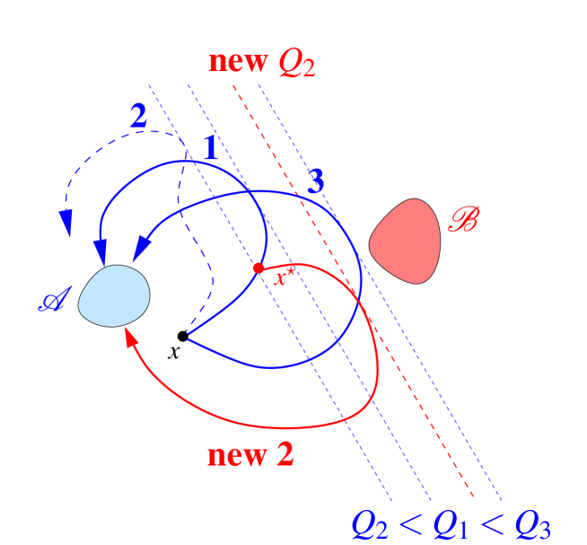
Figure 19: Sketch of the adaptive multilevel splitting algorithm (last particle algorithm) with $N=3$ trajectories. One eliminates the trajectory (trajectory labeled 2 in the sketch) which has the smallest maximum value of $Q$ (denoted $Q_{2}$), and creates a new one (sketched by a red curve) which is resampled from the initial condition from one of the others trajectory chosen randomly (here trajectory 1), and when it crosses the level $Q_{2}$.

Figure B1 gives an illustration of these algorithmic steps. The performance of the algorithm depends crucially on the choice of $\Phi$. One can show that when $\Phi$ has the same isosurfaces than the committor $p({\bf x})$ (which is always true in 1-D), the number of iterations ${\cal K}\sim{\rm Poisson}(-N\log p)$ (Guyader et al., 2011; Simonnet, 2016). Central limit theorems can now be demonstrated in general situations (Bréhier et al., 2016; Cérou and Guyader, 2016) and typically take the form $\sqrt{N}\frac{p-\widehat{p}}{p}\xrightarrow[N\to\infty]{\cal D}{\cal N}(0,|\log p|)$. The advantage of these algorithms is the unbiased estimate they provide. One should be careful however as a bad choice of $\Phi$ may lead to lognormal law with heavy tails and apparent bias (Rolland and Simonnet, 2015). In practice, the larger $N$ the better. A too small value of $N$ not only give results with large variance but also trigger extinction of species by loss of trajectory diversity. One should take advantage of algorithmic variants which eliminate $n\ll N$ trajectories at each step instead of just one. The number of iterations ${\cal K}$ in this case scales like $\frac{N}{n}|\log p|$. Doing so in a parallel environment provide much faster results. This is indeed the strategy used in this paper, where we typically have $N=O(10^{3})$ and $n=O(100)$ on $n$ cores with a speed-up scaling linearly like $O(n)$. In practice, one should also run several i.i.d. algorithmic realisations with different choices of reaction coordinates and consider a set of initial conditions $\mathbf{x}$ rather than a single initial state (see e.g., Cérou et al., 2011).

B.2 Reactive coordinates

There are many possible options to construct reasonable reaction coordinates. The first option is to consider a low-dimensional projection of the system phase space, say on zonal Fourier modes. One can also consider EOFs or wavelets basis to better represent the solutions. In our case, we have chosen the Fourier moduli $|q_{2}|,|q_{3}|,|q_{4}|$ for Fig. 6. One then needs to construct a function $f(|q_{2}|,|q_{3}|,|q_{4}|)\in\mathbb{R}$ such that it describes well the fluctuations of the system. Let $\mathbf{M}$ a projection of the system in the low-dimensional phase space, a natural choice is then to consider $f(\mathbf{M})=\frac{d_{\cal A}}{2d_{\cal B}}$ if $d_{\cal A}\leq d_{\cal B}$ and $f(\mathbf{M})=1-\frac{d_{\cal B}}{2d_{\cal A}}$ if $d_{\cal B}\leq d_{\cal A}$, where $d_{{\cal C}}={\rm dist}(\mathbf{M},{\cal C})$. The function $f$ is equal to zero in the set ${\cal A}$ and one in the set ${\cal B}$. One must be careful as the Euclidian distance may not reflect well the dynamics of the transitions. Moreover if the dimension of the projected phase space is too low, relevant fluctuations may not be seen at all.

B.3 Saddle detection

Once a reactive trajectory reaches a saddle, it should relax, with a probability close to 1, either to the set ${\cal A}$ or the set ${\cal B}$ depending whether it is ”before” or ”after” the saddle. This property is at the basis of the three methods presented.

• The simplest method requires no extra computations and is fairly accurate. Once AMS algorithm has converged, one should simply record the states over which the last branching has occurred. The reason is that these initial conditions all relax (by the ”natural” dynamics, ie the one with probability close to 1) to the target set ${\cal B}$ by the AMS definition whereas previous states relax to ${\cal A}$ again by definition.

• The dichotomy method is more precise than method 1, but it requires extra costly computations as one must reconstruct all AMS trajectories (see Lucarini and Bódai, 2017; Schneider et al., 2007; Willis and Kerswell, 2009, for a similar idea). One proceeds by dichotomy on the reactive trajectories $(\mathbf{X}_{t})_{t\in[0,\tau]}$ by picking initial conditions along the trajectory. For each initial conditions one relaxes the dynamics to decide whether it goes to ${\cal A}$ or ${\cal B}$. The dichotomy provides a critical time, say $t_{s}$, and the saddle is close to $\mathbf{X}_{t_{s}}$. Note that this is correct in probability only, so that one should perform several realisations, and for many AMS trajectories In practice, one realisation is enough since the return time associated to the transition is much larger than the natural relaxation dynamics.

• This method has mainly a theoretical interest. The idea is simply to compute pairs of instantons, anti-instantons and to look for their intersections since they must intersect at saddles and form a so-called figure-eight pattern (see Fig. 10). For reversible dynamics like gradient systems, this approach is irrelevant as the geometric support of an instanton and anti-instanton is the same. In practice, computing anti-instantons is very challenging.

Appendix C Permutations in a channel flow

We investigate here the robustness of the ${\cal S}_{n}$ symmetric group w.r.t. the boundary conditions. We conduct an experiment in a zonally-periodic channel with free-slip boundary conditions, by imposing $q=0$ at the north and south walls and and an additional constraint $\Delta q=0$ for the hyperviscosity. We focus on a parameter regime having three jets ($\beta=8$), and use the same isotropic annular stochastic forcing than in the doubly-periodic case. We generate $O(10)$ i.i.d. realisations starting from the same initial condition $q=0$. We obtain three distinct mirror pairs of solutions w.r.t. the symmetry $y\to-y$ (denoted by a bar), ie a total of 6 different configurations. No additional states have been observed even by increasing the number of realisations. We define $\sigma_{1}$ as the distance between the first and second eastward jet and $\sigma_{2}$, between the second and third eastward jet. The results are shown in Fig. C1 and we call $A,B,C$ the three states (right of Fig. C1) together with their mirror counterparts $\bar{A},\bar{B},\bar{C}$ (upper part of Fig. C1).

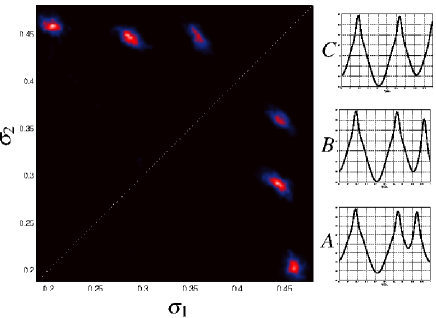
Figure 20: Probability density function $(\sigma_{1},\sigma_{2})$ for the 6 different three alternating jet states, in a zonally-periodic channel with free-slip boundary conditions. The computation used about $10$ independent noise realizations, each starting from rest (zero initial condition). The physical parameters are $\beta=8$ and $\alpha=5\cdot 10^{-4}$. The number of grid points in each direction is $N=400$ using RK4 time scheme for an annular isotropic noise like in the doubly-periodic case at $k_{f}=12$. The diagonal $(\frac{1}{3},\frac{1}{3},\frac{1}{3})$ is shown with a white dotted line.

A close inspection of the numerical values $(\sigma_{1},\sigma_{2},\sigma_{3})$ where $\sigma_{3}=1-\sigma_{1}-\sigma_{2}$, shows that not all permutations are realized. Let us look at the state $A$ with values $(\sigma_{1,A},\sigma_{2,A},\sigma_{3,A})\approx(0.45,0.20,0.34)$, then $C$ is simply $(\sigma_{1,A},\sigma_{3,A},\sigma_{2,A})$, $\bar{A}=(\sigma_{2,A},\sigma_{1,A},\sigma_{3,A})$ and $\bar{C}=(\sigma_{3,A},\sigma_{1,A},\sigma_{2,A})$, giving a total of 4 states. The state $B$ does not correspond to a permutation of the previous states. It has values $(\sigma_{1,B},\sigma_{2,B},\sigma_{3,B})\approx(0.45,0.29,0.27)$. It is almost invariant by permuting $\sigma_{2}$ and $\sigma_{3}$. Note that the boundary conditions impose the presence of either westward or eastward jets on the walls since $q=0$ yields $\frac{du}{dy}=0$, in particular we observe that the states have either two westward jets $(A,B,\bar{A},\bar{B})$ or one eastward and one westward jet $(C,\bar{C})$. The existence of two eastward jets at the north and south walls seems to be forbidden for this value of $\beta$, it has never been observed.

We conclude that the symmetric group appears to be broken into two different subgroups. It suggests a more complex general picture where the symmetries of the problem play a key role in the interaction between the jets. It is plausible for instance that in a four-jet regime, the symmetric group ${\cal S}_{3}$ would emerge as a subgroup.

One of the experiment is shown in the form of an Hovmöller diagram in Fig. C2. A striking transition from $A\to\bar{A}$ takes place through a nucleation inducing a 4-jet state quickly followed by a merging back to the mirror 3-jet state. The solution goes through the perfectly marginally stable symmetry state $(\frac{1}{3},\frac{1}{3},\frac{1}{3})$ (see middle of Fig. C2. Transitions involving internal saddles have not been directly observed and deserve further investigations using the rare event AMS algorithm.

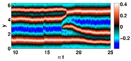
Figure 21: Hovmöller diagram of the zonally averaged zonal velocity in a channel flow showing a transition between $A$ and $\bar{A}$.

References

- Arnold et al. (2012) Arnold, N. P., E. Tziperman, and B. Farrell, 2012: Abrupt transition to strong superrotation driven by equatorial wave resonance in an idealized gcm. Journal of the atmospheric sciences, 69 (2), 626–640.
- Bakas and Ioannou (2014) Bakas, N., and P. Ioannou, 2014: A theory for the emergence of coherent structures in beta-plane turbulence. Journal of Fluid Mechanics, 740, 312–341.
- Berhanu et al. (2007) Berhanu, M., and Coauthors, 2007: Magnetic field reversals in an experimental turbulent dynamo. Eur. Phys. Lett., 77, 59 001.
- Bouchet (2020) Bouchet, F., 2020: Is the boltzmann equation reversible? a large deviation perspective on the irreversibility paradox. Journal of Statistical Physics, 181, 515–550, doi:–10.1007/s10955-020-02588-y˝.
- Bouchet et al. (2014) Bouchet, F., J. Laurie, and O. Zaboronsky, 2014: Langevin dynamics, large deviations and instantons for the quasi-geostrophic model and tzo-dimensional Euler equation. J. Stat. Phys, 156, 1066–1092.
- Bouchet et al. (2018) Bouchet, F., J. Marston, and T. Tangarife, 2018: Fluctuations and large deviations of reynolds stresses in zonal jet dynamics. Physics of Fluids, 30 (1), 015 110.
- Bouchet et al. (2013) Bouchet, F., C. Nardini, and T. Tangarife, 2013: Kinetic theory of jet dynamics in the stochastic barotropic and 2d navier-stokes equations. J. Stat. Phys., 153 (4), 572–625.
- Bouchet et al. (2016) Bouchet, F., C. Nardini, and T. Tangarife, 2016: Non-equilibrium statistical mechanics of the stochastic Navier–Stokes equations and geostrophic turbulence, 34. Warsaw University Press and hal-01143678 https://hal.archives-ouvertes.fr/hal-01143678/document.
- Bouchet et al. (2019) Bouchet, F., J. Rolland, and E. Simonnet, 2019: Rare event algorithm links transitions in turbulent flows with activated nucleations. Physical Review Letters, 122 (7), 074 502.
- Bouchet and Simonnet (2009) Bouchet, F., and E. Simonnet, 2009: Random Changes of Flow Topology in Two-Dimensional and Geophysical Turbulence. Physical Review Letters, 102 (9), 094 504, doi:10.1103/PhysRevLett.102.094504.
- Bréhier et al. (2016) Bréhier, C. E., M. Gazeau, L. Goudenège, T. Lelièvre, and M. Rousset, 2016: Unbiasedness of some Generalized Adaptive Multilevel Splitting algorithms. Annals. of App.Prob.
- Caballero and Huber (2010) Caballero, R., and M. Huber, 2010: Spontaneous transition to superrotation in warm climates simulated by CAM3. Geophys. Res. Lett., 37, L11 701, doi:10.1029/2010GL043468.
- Cérou and Guyader (2007) Cérou, F., and A. Guyader, 2007: Adaptive multilevel splitting for rare events analysis. Stoch. Anal. and Appl., 25, 417–443.
- Cérou and Guyader (2016) Cérou, F., and A. Guyader, 2016: Fluctuation Analysis of Adaptive Multilevel Splitting. Anal.App.Prob., 26(6), 3319–3380.
- Cérou et al. (2011) Cérou, F., A. Guyader, T. Lelièvre, and D. Pommier, 2011: A Multiple Replica Approach to Simulate Reactive Trajectories. J.Chem.Phys., 134, 054 108.
- Cérou et al. (2019) Cérou, F., A. Guyader, and M. Rousset, 2019: Adaptive multilevel splitting: Historical perspective and recent results. Chaos: An Interdisciplinary Journal of Nonlinear Science, 29 (4), 043 108, doi:10.1063/1.5082247, URL http://aip.scitation.org/doi/10.1063/1.5082247.
- Clerke (1893) Clerke, A. M., 1893: A popular history of astronomy during the nineteenth century.
- Constantinou et al. (2014) Constantinou, N. C., B. F. Farrell, and P. J. Ioannou, 2014: Emergence and equilibration of jets in beta-plane turbulence: applications of stochastic structural stability theory. Journal of the Atmospheric Sciences, 71 (5), 1818–1842.
- Danilov and Gurarie (2004) Danilov, S., and D. Gurarie, 2004: Scaling, spectra and zonal jets in beta-plane turbulence. Phys. Fluids, 16, 2592–2603.
- Dansgaard et al. (1993) Dansgaard, W., and Coauthors, 1993: Evidence for general instability of past climate from a 250-kyr ice-core record. Nature, 364, 218–220, doi:10.1038/364218a0.
- Dematteis et al. (2019) Dematteis, G., T. Grafke, M. Onorato, and E. Vanden-Eijnden, 2019: Experimental evidence of hydrodynamic instantons: the universal route to rogue waves. Physical Review X, 9 (4), 041 057.
- Ditlevsen et al. (2007) Ditlevsen, P., K. K. Andersen, and A. Svensson, 2007: The do-climate events are probably noise induced: statistical investigation of the claimed 1470 years cycle. Climate of the Past, 3 (1), 129–134.
- Dritschel and McIntyre (2008) Dritschel, D., and M. McIntyre, 2008: Multiple jets as pv staircases: the phillips effect and the resilience of eddy-transport barriers. Journal of the Atmospheric Sciences, 65 (3), 855–874.
- E and Vanden-Eijnden (2006) E, W., and E. Vanden-Eijnden, 2006: Towards a Theory of Transition Paths. J.Stat.Phys., 123, 504–523.
- Ebener et al. (2018) Ebener, L., G. Margazoglou, J. Friedrich, L. Biferale, and R. Grauer, 2018: Instanton based importance sampling for rare events in stochastic PDE. arXiv:1812.03543.
- Ebener et al. (2019) Ebener, L., G. Margazoglou, J. Friedrich, L. Biferale, and R. Grauer, 2019: Instanton base importance sampling for rare events in stochastic pdes. Chaos: An Interdisciplinary Journal of Nonlinear Science.
- Farrel and Ioannou (2007) Farrel, B. F., and P. J. Ioannou, 2007: Structure and Spacing of Jets in Barotropic Turbulence. J. Atmos. Sci., 64, 3652–3664.
- Farrell and Ioannou (2003) Farrell, B. F., and P. J. Ioannou, 2003: Structural stability of turbulent jets. Journal of Atmospheric Sciences, 60, 2101–2118.
- Freidlin and Wentzell (1984) Freidlin, M. I., and A. D. Wentzell, 1984: Random Perturbations of Dynamical Systems, volume 260 of Grundlehren der Mathematischen Wissenschaften. Springer-Verlag, New York.
- Galperin and Read (2019) Galperin, B., and P. Read, Eds., 2019: Zonal Jets: Phenomenology, Genesis, and Physics. Cambridge University Press, doi:10.1017/9781107358225.
- Galperin et al. (2001) Galperin, B., S. Sukoriansky, and H.-P. Huang, 2001: Universal spectrum of zonal flows on giant planets. Phys. Fluids, 13, 1545.
- Galperin et al. (2014) Galperin, B., R. M. Young, S. Sukoriansky, N. Dikovskaya, P. L. Read, A. J. Lancaster, and D. Armstrong, 2014: Cassini observations reveal a regime of zonostrophic macroturbulence on jupiter. Icarus, 229, 295–320.
- Grafke et al. (2015) Grafke, T., R. Grauer, and T. Schäfer, 2015: The instanton method and its numerical implementation in fluid mechanics. J.Phys.A:Math.Theor., 48, 333 001.
- Grafke and Vanden-Eijnden (2019) Grafke, T., and E. Vanden-Eijnden, 2019: Numerical computation of rare events via large deviation theory. Chaos: An Interdisciplinary Journal of Nonlinear Science, 29 (6), 063 118.
- Grebogi et al. (1983) Grebogi, C., E. Ott, and J. A. Yorke, 1983: Crises, sudden changes in chaotic attractors and transient chaos. Physica D, 7, 181–200.
- Guyader et al. (2011) Guyader, A., N. Hengartner, and E. M.-L. ber, 2011: Simulation and Estimation of Extreme Quantiles and Extreme Probabilities. Appl. Math. Optim., 64, 171–196.
- Haidvogel and Held (1981) Haidvogel, D., and I. Held, 1981: Homogeneous quasi-geostrophic turbulence driven by a uniform temperature gradient. J. Atmos. Sci., 37, 2644–2660.
- Hartmann et al. (2013) Hartmann, C., R. Banisch, M. Sarich, T. Badowski, and C. Schütte, 2013: Characterization of Rare Events in Molecular Dynamics. Entropy, 16 (1), 350–376, doi:10.3390/e16010350, URL http://www.mdpi.com/1099-4300/16/1/350.
- Held (1999) Held, I. M., 1999: Equatorial superrotation in Earth-like atmospheric models. Bernhard Haurwitz Memorial Lecture.
- Herbert et al. (2020) Herbert, C., R. Caballero, and F. Bouchet, 2020: Atmospheric bistability and abrupt transitions to superrotation: Wave–jet resonance and hadley cell feedbacks. Journal of the Atmospheric Sciences, 77 (1), 31–49.
- H.L.Kuo (1949) H.L.Kuo, 1949: Dynamics instability of two-dimensional nondivergent flow in a barotropic atmosphere. J.Fluid.Mech., 6, 105–122.
- Huang and Robinson (1998) Huang, H.-P., and W. A. Robinson, 1998: Two-dimensional turbulence and persistent zonal jets in a global barotropic model. Journal of the atmospheric sciences, 55 (4), 611–632.
- Ingersoll and Pollard (1982) Ingersoll, A. P., and D. Pollard, 1982: Motion in the interiors and atmospheres of jupiter and saturn: Scale analysis, anelastic equations, barotropic stability criterion. Icarus, 52 (1), 62–80.
- Jougla and Dritschel (2017) Jougla, T., and D. G. Dritschel, 2017: On the energetics of a two-layer baroclinic flow. Journal of Fluid Mechanics, 816, 586–618.
- Kahn and Harris (1951) Kahn, H., and T. Harris, 1951: Estimation of particle transmission by random sampling. Natl. Bur. Stand., Appl. Math. Ser., 12, 27–30.
- Kaspi and Flierl (2007) Kaspi, Y., and G. R. Flierl, 2007: Formation of Jets by Baroclinic Instability on Gas Planet Atmospheres. J. Atmos. Sci., 64, 3177–3194.
- Laurie et al. (2014) Laurie, J., G. Boffetta, G. Falkovich, I. Kolokolov, and V. Lebedev, 2014: Universal profile of the vortex condensate in two-dimensional turbulence. Physical review letters, 113 (25), 254 503.
- Laurie and Bouchet (2015) Laurie, J., and F. Bouchet, 2015: Computation of rare transitions in the barotropic quasi-geostrophic equations. New J. of Phys., 17, 015 009.
- Lee (1997) Lee, S., 1997: Maintenance of multiple jets in a barotropic flow. J. Atmos. Sci., 54, 1726–1738.
- Lee (2005) Lee, S., 2005: Baroclinic multiple zonal jets on the sphere. Journal of the atmospheric sciences, 62 (7), 2484–2498.
- Lemasquerier et al. (2020) Lemasquerier, D., B. Favier, and M. L. Bars, 2020: Zonal jets at the laboratory scale: hysteresis and rossby waves resonance. arXiv preprint arXiv:2008.10304.
- Lestang et al. (2020) Lestang, T., F. Bouchet, and E. Lévêque, 2020: Numerical study of extreme mechanical force exerted by a turbulent flow on a bluff body by direct and rare-event sampling techniques. Journal of Fluid Mechanics, 895.
- Lorenz (1967) Lorenz, E. N., 1967: The nature and theory of the general circulation of the atmosphere. World Meteorological Organization.
- Lucarini and Bódai (2017) Lucarini, V., and T. Bódai, 2017: Edge states in the climate system: exploring global instabilities and critical transitions. Nonlinearity, 30, 32–66.
- Manfroi and Young (1999) Manfroi, A., and W. Young, 1999: Slow evolution of zonal jets on the beta plane. Journal of the Atmospheric Sciences, 56, 784–800.
- Maragliano et al. (2010) Maragliano, L., G. Cottone, G. Ciccotti, and E. Vanden-Eijnden, 2010: Mapping the Network of Pathways of CO Diffusion in Myoglobin. J.Am.Chem.Soc., 132(3), 1010–1017.
- Marcus (2004) Marcus, P., 2004: Prediction of a global climate change on Jupiter. Nature, 428, 828–831.
- Marcus and Lee (1998) Marcus, P., and C. Lee, 1998: A model for eastward and westward jets in laboratory experiments and planetary atmospheres. Physics of Fluids, 10 (6), 1474–1489.
- Metzner et al. (2009) Metzner, P., C. Schütte, and E. Vanden-Eijnden, 2009: Transition path theory for markov jump processes. Multiscale Modeling & Simulation, 7 (3), 1192–1219.
- Onsager and Machlup (1953) Onsager, L., and S. Machlup, 1953: Fluctuations and irreversible processes. Phys. Rev., 91, 1505–1512.
- P. Del Moral (2004) P. Del Moral, 2004: Feynman-Kac formulae, Genealogical and interacting particle systems with applications. Probability and Applications, Springer-Verlag, New York.
- Paillard (1998) Paillard, D., 1998: The timing of pleistocene glaciations from a simple multiple-state climate model. Nature, 391 (6665), 378–381.
- Panetta (1993) Panetta, R. L., 1993: Zonal Jets in Wide baroclinically unstable regions: persistence and scale selection. J. Atmos. Sci., 50, 2073–2106.
- Parker and Krommes (2013) Parker, J. B., and J. A. Krommes, 2013: Zonal flow as pattern formation. Physics of Plasmas, 20 (10), 100 703.
- Phillips (1951) Phillips, N., 1951: A simple three-dimensional model for the study of large-scale extratropical flow patterns. J. Meteor., 8, 381–394.
- Pierrehumbert et al. (2011) Pierrehumbert, R., D. Abbot, A. Voigt, and D. Koll, 2011: Climate of the neoproterozoic. Annual Review of Earth and Planetary Sciences, 39.
- Plotkin et al. (2019) Plotkin, D. A., R. J. Webber, M. E. O’Neill, J. Weare, and D. S. Abbot, 2019: Maximizing simulated tropical cyclone intensity with action minimization. Journal of Advances in Modeling Earth Systems, 11 (4), 863–891.
- Porco et al. (2004) Porco, C. C., and Coauthors, 2004: Cassini imaging science: Instrument characteristics and anticipated scientific investigations at saturn. Space Science Reviews, 115 (1-4), 363–497.
- Qiu and Miao (2000) Qiu, B., and W. Miao, 2000: Kuroshio path variations south of Japan: Bimodality as a self-sustained internal oscillation. J. Phys. Oceanogr., 30, 2124–2137.
- Ragone and Bouchet (2019) Ragone, F., and F. Bouchet, 2019: Computation of extreme values of time averaged observables in climate models with large deviation techniques. Journal of Statistical Physics, 1–29.
- Ragone et al. (2018) Ragone, F., J. Wouters, and F. Bouchet, 2018: Computation of extreme heat waves in climate models using a large deviation algorithm. PROCEEDINGS OF THE NATIONAL ACADEMY OF SCIENCES OF THE UNITED STATES OF AMERICA, 115 (1), 24–29, doi:–10.1073/pnas.1712645115˝.
- Rahmstorf (2002) Rahmstorf, S., 2002: Ocean circulation and climate during the past 120,000 years. Nature, 419, 207–214.
- Ravelet et al. (2004) Ravelet, F., L. Marié, A. Chiffaudel, and F. Daviaud, 2004: Multistability and memory effect in a highly turbulent flow: experimental evidence for a global bifurcation. Phys.Rev.Lett., 93, 164 501.
- Read et al. (2020a) Read, P., D. Kennedy, N. Lewis, H. Scolan, F. Tabataba-Vakili, Y. Wang, S. Wright, and R. Young, 2020a: Baroclinic and barotropic instabilities in planetary atmospheres: energetics, equilibration and adjustment. Nonlinear Processes in Geophysics, 27 (2), 147–173.
- Read et al. (2020b) Read, P. L., R. M. Young, and D. Kennedy, 2020b: The turbulent dynamics of jupiter’s and saturn’s weather layers: order out of chaos? Geoscience Letters, 7 (1), 1–18.
- Rogers (1995) Rogers, J. H., 1995: The Giant Planet Jupiter. Cambridge University Press, 418 pp.
- Rolland et al. (2016) Rolland, J., F. Bouchet, and E. Simonnet, 2016: Computing transition rates for the 1-D stochastic Ginzburg–Landau–Allen–Cahn equation for finite-amplitude noise with a rare event algorithm . J. Stat. Phys., 162, 277–311.
- Rolland and Simonnet (2015) Rolland, J., and E. Simonnet, 2015: Statistical behavior of adaptive multilevel algorithm in simple models. J.Comput.Phys., 283, 541–557.
- Rosenbluth and Rosenbluth (1955) Rosenbluth, M., and A. Rosenbluth, 1955: Monte Carlo calculation of the average extension of molecular chains. J.Chem.Phys., 23, 356–359.
- Schmeits and Dijkstra (2001) Schmeits, M. J., and H. A. Dijkstra, 2001: Bimodal behavior of the Kuroshio and the Gulf Stream. J. Phys. Oceanogr., 31, 3435–3456.
- Schneider et al. (2007) Schneider, T. M., B. Eckhardt, and J. A. Yorke, 2007: Turbulence transition and the edge of chaos in pipe flow. Physical review letters, 99 (3), 034 502.
- Simon et al. (2015) Simon, A. A., M. H. Wong, and G. S. Orton, 2015: First results from the hubble opal program: Jupiter in 2015. Astrophys. J., 812, 55–63.
- Simonnet (2016) Simonnet, E., 2016: Combinatorial analysis of the adaptive last particle method. Stat. Comp., 26, 211–230.
- Srinivasan and Young (2014) Srinivasan, K., and W. Young, 2014: Reynolds stress and eddy diffusivity of -plane shear flows. Journal of the Atmospheric Sciences, 71 (6), 2169–2185.
- Srinivasan and Young (2011) Srinivasan, K., and W. R. Young, 2011: Zonostrophic Instability. J. Atmos. Sci., 69 (5), 1633–1656.
- Tobias and Marston (2013) Tobias, S., and J. Marston, 2013: Direct statistical simulation of out-of-equilibrium jets. Phys. Rev. Lett., 110 (10), 104 502.
- Tziperman and Farrell (2009) Tziperman, E., and B. Farrell, 2009: Pliocene equatorial temperature: Lessons from atmospheric superrotation. Paleoceanography, 24, PA1101, doi:10.1175/1520-0469(2000)057¡1937:RFNCAT¿2.0.CO;2.
- Vallis and Maltrud (1993) Vallis, G. K., and M. E. Maltrud, 1993: Generation of mean flows and jets on a beta plane and over topography. J. Phys. Oceanogr., 23, 1346–1362.
- Webber et al. (2019) Webber, R. J., D. A. Plotkin, M. E. O’Neill, D. S. Abbot, and J. Weare, 2019: Practical rare event sampling for extreme mesoscale weather. Chaos: An Interdisciplinary Journal of Nonlinear Science, 29 (5), 053 109, doi:10.1063/1.5081461, URL https://aip.scitation.org/doi/full/10.1063/1.5081461.
- Williams (1979) Williams, G. P., 1979: Planetary ciruclations. 2: The Jovian quasi-geostrophic regime. J. Atmos. Sci., 36, 932–968.
- Williams (2003) Williams, G. P., 2003: Jovian Dynamics. Part III: Multiple, Migrating, and Equatorial Jets. J. Atmos. Sci., 60, 1270–1296.
- Willis and Kerswell (2009) Willis, A. P., and R. R. Kerswell, 2009: Turbulent dynamics of pipe flow captured in a reduced model: puff relaminarization and localized “edge” states. Journal of fluid mechanics, 619, 213–233.
- Woillez and Bouchet (2019) Woillez, E., and F. Bouchet, 2019: Barotropic theory for the velocity profile of jupiter’s turbulent jets: an example for an exact turbulent closure. Journal of Fluid Mechanics, 860, 577–607.
- Woillez and Bouchet (2020) Woillez, E., and F. Bouchet, 2020: Instantons for the destabilization of the inner solar system. Physical Review Letters, 125 (2), 021 101.
- Wouters and Bouchet (2016) Wouters, J., and F. Bouchet, 2016: Rare event computation in deterministic chaotic systems using genealogical particle analysis. Journal of Physics A: Mathematical and Theoretical, 49 (37), 374 002.