Computation of Parameter Dependent Robust Invariant Sets for LPV Models with Guaranteed Performance

Abstract

This paper presents an iterative algorithm to compute a Robust Control Invariant (RCI) set, along with an invariance-inducing control law, for Linear Parameter-Varying (LPV) systems. As real-time measurements of the scheduling parameters are typically available, we allow the RCI set description and the invariance-inducing controller to be scheduling parameter dependent. Thus, the considered formulation leads to parameter-dependent conditions for the set invariance, which are replaced by sufficient Linear Matrix Inequalities (LMIs) via Polya’s relaxation. These LMI conditions are then combined with a novel volume maximization approach in a Semidefinite Programming (SDP) problem, which aims at computing the desirably large RCI set. Besides ensuring invariance, it is also possible to guarantee performance within the RCI set by imposing a chosen quadratic performance level as an additional constraint in the SDP problem. Using numerical examples, we show that the presented iterative algorithm can generate RCI sets for large parameter variations where commonly used robust approaches fail.

, , ,

1 Introduction

RCI set is a set of system states where a feasible control input always exists, which restricts the future states within the set in the presence of disturbances. These sets have become an essential tool for controller synthesis and stability analysis of linear and nonlinear systems Blanchini & Miani (2015); Raković & Baric (2010); Fiacchini et al. (2010); Bravo et al. (2005).

When computing RCI sets for LPV systems, a common practice is to treat the scheduling parameters as bounded uncertainties Hanema et al. (2020); Miani & Savorgnan (2005); Gupta et al. (2019); Nguyen et al. (2015). Moreover, the invariance inducing control laws are typically assumed to be only state-dependent, without exploiting the observed scheduling parameter information. In this way, the obtained RCI sets can be potentially conservative and, in the worst case, even empty. Thus, to exploit the information on the scheduling parameters, we propose a new algorithm to compute scheduling parameter-dependent RCI sets and invariance inducing control laws for LPV systems. In this paper, such sets are termed as parameter-dependent RCI (PD-RCI) sets and parameter-dependent control laws (PDCLs), respectively. The advantages of using a PDCL and PD-RCI set are:

• PDCL: these control laws can stabilize LPV systems that may not be stabilizable by treating the parameters as unknown bounded uncertainties Blanchini et al. (2007). Moreover, when computing the RCI sets, keeping PDCL as an optimization variable provides extra degrees of freedom. We remark that a similar construction was proposed in a robust framework in Blanco et al. (2010); Gupta et al. (2019); Liu et al. (2019).

• PD-RCI sets: Scheduling parameters affect the system’s time evolution, and thus the set of states for which invariance can be achieved. Therefore, only considering fixed (or parameter-independent) RCI set description for all scheduling parameters could be restrictive and may lead to conservative (volume-wise) sets. This restrictiveness motivates us to allow the RCI set description to be parameter-dependent.

This paper presents an iterative algorithm to compute a PD-RCI set of desirably large volume and PDCL for the LPV systems. We also present a method to compute PD-RCI sets within which a desired quadratic performance can be guaranteed. The representational complexity of the PD-RCI sets can be predefined. The related LMI conditions for invariance are derived by employing Finsler’s lemma and Polya’s relaxation. These conditions are constructed to ensure invariance for all future (unknown) values of the scheduling parameters. In order to obtain an RCI set with a desirably large volume, we present a volume maximization heuristic based on the theory of Monte-Carlo integration and its convex relaxations.

The paper is organized as follows: In Section 3, we formalize the problem of computing PD-RCI set and PDCL. Sufficient parameter-dependent conditions for invariance and performance are derived in Section 4, and corresponding LMI conditions in Section 5. Using these conditions, an iterative algorithm to compute desirably large RCI sets is proposed in Section 6. Two case studies are reported in Section 7

Notation: We use $\mathbb{D}^{n}_{+}\in\mathbb{R}^{n\times n}$ to denote the set of all diagonal matrices with positive diagonal entries. $I$ and $e_{i}$ represent the identity matrix and its $i$-th column, and vector of ones is denoted by $\bm{1}$, with dimension defined by the context. $X\succ 0\,(\succeq 0)$ denotes a positive (semi) definite matrix $X$. For compactness, in the text $*$’s will represent matrix’s entries that are uniquely identifiable from symmetry, and for some square matrix $X$, $\mathsf{He}(X)=X+X^{T}$. We use $X^{k}$ and $x^{k}$ to represent a matrix and a vector of appropriate dimension indexed with ‘$k$’. Let $L(X^{k},Y^{l},\bar{\Theta},\Theta)$ be a matrix-valued function, where $X^{k}$ and $Y^{l}$ represent all matrices indexed with ‘$k$’ and ‘$l$’, and $\bar{\Theta},\Theta$ are some arbitrary matrices. We use $\bm{L}^{k,l}(\bar{\Theta},\Theta)=L(X^{k},Y^{l},\bar{\Theta},\Theta)$, $\bm{L}^{l,k}(\bar{\Theta},\Theta)=L(X^{l},Y^{k},\bar{\Theta},\Theta)$ and $\bm{L}^{k,k}(\bar{\Theta},\Theta)=L(X^{k},Y^{k},\bar{\Theta},\Theta)$.

2 Preliminaries

We recall two existing results which will be used in the paper.

Lemma 1 (Finsler’s Lemma).

Let $\xi\in\bm{\Xi}\subseteq\mathbb{R}^{N_{\xi}}$, $\Phi:\bm{\Xi}\rightarrow\mathbb{R}^{n\times n}$ and $\Delta:\bm{\Xi}\rightarrow\mathbb{R}^{m\times n}$. Then the following statements are equivalent (Ishihara et al., 2017):

1. For each $\xi\in\bm{\Xi}$, $y^{T}\Phi(\xi)y\succ 0,\;\forall\Delta(\xi)y=0,\;y\neq 0$.

2. For each $\xi\in\bm{\Xi}$, $\exists\Psi\in\mathbb{R}^{n\times m}$ such that
            $\Phi(\xi)+\Psi(\xi)\Delta(\xi)+\Delta(\xi)^{T}\Psi(\xi)^{T}\succ 0$.

Lemma 2 (Linearization Lemma).

Let $\mathcal{L}\in\mathbb{R}^{m\times n}$ be any arbitrary matrix and $\mathcal{M}\in\mathbb{R}^{m\times m}$ be a positive definite matrix. The following relation always holds for any arbitrary matrix $\mathcal{Y}\in\mathbb{R}^{m\times n}$ (Gupta et al., 2019)

$$\mathcal{L}^{T}\mathcal{M}^{-1}\mathcal{L}\succeq\mathcal{L}^{T}\mathcal{Y}+\mathcal{Y}^{T}\mathcal{L}-\mathcal{Y}^{T}\mathcal{M}\mathcal{Y}\vspace{-0.2cm}$$ (1)

The result can be easily verified by adding a residual term $(\mathcal{L}-\mathcal{M}\mathcal{Y})^{T}\mathcal{M}^{-1}(\mathcal{L}-\mathcal{M}\mathcal{Y})$ on the r.h.s of (1). This lemma is utilized to resolve the non-linear matrix inequalities, i.e., the non-linear term on the l.h.s. of (1) can be replaced with linear (in variables $\mathcal{L},\mathcal{M}$) matrix term on r.h.s., by appropriate choice of $\mathcal{Y}$.

Remark 1.

[Successive linearization] Though $\mathcal{Y}$ can be any arbitrary matrix of compatible dimension, in order to reduce conservatism due to linearization, we suggest successive linearization approach. An appropriate choice would be to select $\mathcal{Y}=\mathcal{M}^{-1}_{0}\mathcal{L}_{0}$, where $\mathcal{M}_{0}$, $\mathcal{L}_{0}$ are the values of $\mathcal{M}$, $\mathcal{L}$ obtained from previous iteration. Thus the nonlinearity can be resolved iteratively in which the residual term shrinks with each iteration. Notice that (1) holds with equality if $\mathcal{L}=\mathcal{L}_{0}$ and $\mathcal{M}=\mathcal{M}_{0}$, this will be a key property towards proving recursive feasibility of our iterative schemes proposed in this paper.

3 Problem Statement

Let us consider a discrete-time polytopic LPV system:

$$x(t\!+\!1)\! =\!\mathcal{A}(\xi(t))x(t)+\mathcal{B}(\xi(t))u(t)+\mathcal{E}(\xi(t))w(t),$$ (2)

$$z(t)\! =\!\mathcal{C}(\xi(t))x(t)+\mathcal{D}(\xi(t))u(t),\vspace{-0.2cm}$$ (3)

where time index $t\in\mathbb{Z}_{+}$, $x(t)\in\mathbb{R}^{n_{x}}$ and $z(t)\in\mathbb{R}^{n_{z}}$ are the current state and the output vectors, $x(t+1)$ is the successor state, and $u(t)\in\mathbb{R}^{n_{u}}$ and $w(t)\in\mathbb{R}^{n_{w}}$ are the control and the disturbance input vectors, respectively. The system matrices $\mathcal{A}(\xi(t))$, $\mathcal{B}(\xi(t))$, $\mathcal{C}(\xi(t))$, $\mathcal{D}(\xi(t))$ and $\mathcal{E}(\xi(t))$ depend on the time-varying scheduling parameter $\xi(t)$, which takes value in unit simplex,

$$\bm{\Xi}=\left\{\xi\in\mathbb{R}^{N_{\xi}}:\sum_{k=1}^{N_{\xi}}\xi_{k}=1,\ \ \xi_{k}\geq 0\right\}.\vspace{-0.2cm}$$ (4)

It is assumed that the current value of $\xi(t)$ is always available. The polytopic system matrices are given by

$$\begin{bmatrix}\mathcal{A}(\xi(t))\!\!&\!\!\mathcal{B}(\xi(t))\!\!&\!\!\mathcal{E}(\xi(t))\\ \mathcal{C}(\xi(t))\!\!&\!\!\mathcal{D}(\xi(t))\!&\!0\end{bmatrix}\!\!=\!\!\sum_{k=1}^{N_{\xi}}\xi_{k}(t)\begin{bmatrix}A^{k}&B^{k}&E^{k}\\ C^{k}&D^{k}&0\end{bmatrix},\vspace{-0.2cm}$$ (5)

with $A^{k},B^{k},C^{k},D^{k},E^{k}$ real matrices of compatible dimensions. The system is subjected to the following polytopic state/input constraints and bounded disturbance:

$$\begin{matrix}\bm{\mathcal{X}}_{u}&=&\left\{(x,u):H_{x}x(t)+H_{u}u(t)\leq\mathbf{1}\right\},\\ \bm{\mathcal{W}}&=&\left\{w:-\mathbf{1}\leq Gw(t)\leq\mathbf{1}\right\}.\end{matrix}\vspace{-0.2cm}$$ (6)

where $H_{x}\in\mathbb{R}^{n_{h}\times n_{x}}$, $H_{u}\in\mathbb{R}^{n_{h}\times n_{u}}$ and $G\in\mathbb{R}^{n_{g}\times n_{w}}$ are given matrices. In this paper, we want to compute a 0-symmetric PD-RCI set with a predefined complexity $n_{p}$ described as

$$\bm{\mathcal{S}}(\xi(t))\!=\!\left\{x\in\mathbb{R}^{n_{x}}:-\bm{1}\!\leq\!\mathcal{P}(\xi(t))W^{-1}x(t)\!\leq\!\bm{1}\right\},\vspace{-0.2cm}$$ (7)

where $\mathcal{P}(\xi(t))\triangleq\sum_{k=1}^{N_{\xi}}\xi_{k}(t)P^{k}$, $P^{k}\in\mathbb{R}^{n_{p}\times n_{x}}$ and $W\in\mathbb{R}^{n_{x}\times n_{x}}$. The presented parameterization of PD-RCI set will be justified when we formalize the problem. Note that, if $P^{k}=P$ for all $k=1,\ldots,N_{\xi}$, then $\mathcal{P}(\xi(t))=P$, which is similar to the (parameter-independent) RCI set description considered in Gupta & Falcone (2019); Liu et al. (2019). In order to have a non-empty and bounded set $\bm{\mathcal{S}}(\xi(t))$, the matrix $W$ should be invertible and $\mathsf{Rank}(\mathcal{P}(\xi(t)))=n_{x},\;\forall\xi\in\bm{\Xi}$. This will be later guaranteed by proper LMI conditions. Furthermore, invariance in the set $\bm{\mathcal{S}}(\xi(t))$ is achieved with a PDCL, which is not known a priori and expressed as

$$u(t)=\mathcal{K}(\xi(t))x(t),\vspace{-0.2cm}$$ (8)

where $\mathcal{K}(\xi(t))\triangleq\sum_{k=1}^{N_{\xi}}\xi_{k}(t)K^{k}$ and $K^{k}\in\mathbb{R}^{n_{u}\times n_{x}}$. The closed-loop representation of the system (2) and (3) with the controller (8) can be written as

$$x(t\!\!+\!\!1)\!\!=\!\!\overbrace{(\!\mathcal{A}(\xi(t))\!+\!\mathcal{B}(\xi(t)\!)\mathcal{K}(\xi(t))}^{\mathcal{A_{K}}(\xi(t))}x(t)\!\!+\!\!\mathcal{E}(\xi(t))w(t),$$ (9)

$$z(t)=\overbrace{(\mathcal{C}(\xi(t))\!+\!\mathcal{D}(\xi(t))\mathcal{K}(\xi(t))}^{\mathcal{C_{K}}(\xi(t))}x(t).\vspace{-0.2cm}$$ (10)

To the best of authors’ knowledge, there is no related work which computes the described PD-RCI set. Thus we first formalize the definition of the set by adapting the standard definition of the RCI set to the LPV setting in the sequel.

Definition 1.

We say a set $\bm{\mathcal{S}}(\xi(t))$ is a PD-RCI set if for any given $\xi(t)\in\bm{\Xi}$ and each $x(t)\in\bm{\mathcal{S}}(\xi(t))$

$$\mathcal{A_{K}}(\xi(t))\bm{\mathcal{S}}(\xi(t))\oplus\mathcal{E}(\xi(t))\bm{\mathcal{W}}\subseteq\bm{\mathcal{S}}(\xi(t+1)),\forall\xi(t\!+\!1)\in\bm{\Xi}\vspace{-0.2cm}$$ (11)

Condition (11) should be satisfied for $\forall\xi(t+1)\in\bm{\Xi}$ since $\xi(t+1)$ is unknown at time $t$, which also implies $x(t+1)\in\bigcap_{\forall\xi(t+1)\in\bm{\Xi}}\bm{\mathcal{S}}(\xi(t+1))$. The computed set $\bm{\mathcal{S}}(\xi(t))$ and the PDCL $\mathcal{K}(\xi(t))$ should obey the system constraints (6), which implies

$$\bm{\mathcal{S}}(\xi(t))\subseteq\bm{\mathcal{X}}(\xi(t)),\vspace{-0.2cm}$$ (12)

where $\bm{\mathcal{X}}(\xi(t))\!=\!\left\{x:(H_{x}\!+\!H_{u}\mathcal{K}(\xi(t)))x(t)\leq\mathbf{1}\right\}$. In classical formulation, RCI set description is independent of the scheduling parameters and is fixed for all $\xi\in\bm{\Xi}$. On the other hand, for PD-RCI set (7), different values of initial parameter $\xi(t)\in\bm{\Xi}$ provide different slices of the set $\bm{\mathcal{S}}(\xi(t))$ for which the invariance can be achieved. Thus, PD-RCI set provides more flexibility in finding the set of initial states for which invariance can be achieved.

In some applications (e.g., MPC), it may be desirable to have a guaranteed performance within the PD-RCI sets for the closed loop system (9) and (10). For this purpose, we consider quadratic performance constraint

$$\sum_{t=0}^{\infty}\left\|z(t)\right\|^{2}_{2}\leq\gamma,\;0\leq\gamma<\infty.\vspace{-0.2cm}$$ (13)

Here w.l.o.g., we assume that performance is measured from time $t=0$. Note that (13) can be only satisfied if $w(t)=0,\ \forall t\geq 0$ (or $w(t)$ eventually becomes zero after certain time). Hence, we will assume $w(t)=0$ only when performance constraints are considered.

Our aim is to compute $\mathcal{P}(\xi(t))$, $W$ and $\mathcal{K}(\xi(t))$, which define the PD-RCI set (7) and the invariance inducing controller (8). We remark that, with $W=I$, computation of $\mathcal{P}(\xi(t))$ and $\mathcal{K}(\xi(t))$ results in a highly non-linear problem. Indeed, introduction of the matrix $W$ helps overcome the nonlinearity by decomposing the problem into two subproblems described as follows. The first subproblem aims to compute $W$ and $\mathcal{K}(\xi(t))$ for given parameter-independent matrix $P$. The second subproblem, aims to compute the parameter-dependent matrix $\mathcal{P}(\xi(t))$ and updated controller $\mathcal{K}(\xi(t))$, for a given matrix $W$ obtained from solving the first subproblem. The two subproblems are formalized as follows.

Problem 1.

For a given matrix $P_{init}\in\mathbb{R}^{n_{p}\times n_{x}}$ such that $\mathcal{P}(\xi(t))=P_{init}$ and the discrete-time system (2) subject to constraints (6), find a matrix $W$ and the control law $\mathcal{K}(\xi(t))$ that satisfies conditions (11), (12) and (13) for any arbitrary variation of $\xi(t)\in\bm{\Xi},\forall t\geq 0$.

Problem 2.

For a given matrix $W$ and the discrete-time system (2) subject to constraints (6), find the matrix $\mathcal{P}(\xi(t))$ and the control law $\mathcal{K}(\xi(t))$ that satisfies conditions (11), (12) and (13) for any arbitrary variation of $\xi(t)\in\bm{\Xi},\forall t\geq 0$.

Observe that by solving Problem 1, we obtain an RCI set which is independent of the parameter $\xi(t)$ since $\mathcal{P}(\xi(t))=P_{init}$. In order to obtain a PD-RCI set $\bm{\mathcal{S}}(\xi(t))$, we need to solve Problem 1 and Problem 2 sequentially. In both problems, (13) is imposed only if performance is desired. Even though we present our formulation in the form of feasibility problems, our final goal is to design algorithms to compute a desirably large PD-RCI set. In the next section, we derive matrix inequality conditions for (11), (12) and (13). These conditions will be later used to obtain LMI conditions which solve Problem 1 and Problem 2.

4 Sufficient Parameter Dependent Conditions for Invariance and Performance

For brevity, we will suppress the time dependent representation of the considered signals and use superscript ‘⁺’ to indicate successor of $x(t)$ and $\xi(t)$. The arguments of the matrices $\mathcal{A_{K}}(\xi)$, ${\mathcal{E}}(\xi)$, $\mathcal{C_{K}}(\xi)$, $\mathcal{P}(\xi)$ and the set $\bm{\mathcal{S}}(\xi)$ will be suppressed and recalled whenever necessary.

4.1 Parameter dependent conditions for invariance and system constrains

From (7) and (11), a set $\bm{\mathcal{S}}(\xi)$ is invariant, if for a given $\xi\in\bm{\Xi}$ and for each $x\in\bm{\mathcal{S}}(\xi)$, for $i=1,\ldots,n_{p}$

$$\!\!(1\!-\!(e_{i}^{T}\mathcal{P}(\xi^{+})W^{-1}x^{+})^{2})\!\geq\!0,\forall(w,\xi^{+})\!\in\!(\bm{\mathcal{W}},\bm{\Xi}),$$ (14)

Using S-procedure (Pólik & Terlaky (2007)), (6) and (7), we can rewrite condition (14) as,

$$\phi_{i}(1-(e_{i}^{T}\mathcal{P}(\xi^{+})W^{-1}x^{+})^{2})\geq\!\\ (\bm{1}\!-\!\mathcal{P}W^{-1}x)^{T}\Lambda_{i}(\bm{1}\!+\!\mathcal{P}W^{-1}x)\!+\!(\bm{1}\!-\!Gw)^{T}\Gamma_{i}(\bm{1}\!+\!Gw),\\ \forall(w,\xi^{+})\in(\bm{\mathcal{W}},\bm{\Xi}),i=1,\ldots,n_{p},\vspace{-0.2cm}$$ (15)

where $\phi_{i}\in\mathbb{R}_{+}$, $\Lambda_{i}\in\mathbb{D}_{+}^{n_{p}}$ and $\Gamma_{i}\in\mathbb{D}_{+}^{n_{g}}$. The vector $x^{+}$ in (15) should satisfy (9), hence (15) can be written as

$$\chi_{1}^{T}\begin{bmatrix}r_{i}&0&0&0\\ 0&W^{-T}\mathcal{P}^{T}\Lambda_{i}\mathcal{P}W^{-1}&0&0\\ 0&0&G^{T}\Gamma_{i}G&0\\ 0&0&0&-p_{i}\end{bmatrix}{\chi_{1}}\succeq 0,\;\\ \forall\begin{bmatrix}0&-\mathcal{A_{K}}&-\mathcal{E}&I\end{bmatrix}\chi_{1}=0,$$ (16)

where $\chi_{1}=\begin{bmatrix}1&x^{T}&w^{T}&(x^{+})^{T}\end{bmatrix}^{T}$, $r_{i}=\phi_{i}-\bm{1}^{T}\Lambda_{i}\bm{1}-\bm{1}^{T}\Gamma_{i}\bm{1}$ and $p_{i}=W^{-T}\mathcal{P}^{T}(\xi^{+})e_{i}\phi_{i}e_{i}^{T}\mathcal{P}(\xi^{+})W^{-1}$. We will utilize Lemma 1 to derive sufficient condition for (16). In particular, by choosing $\Psi_{i}(\xi)=\begin{bmatrix}0&0&0&\mathcal{V}_{i}(\xi)^{-1}\end{bmatrix}^{T}$ in Lemma 1, where $\mathcal{V}_{i}(\xi)=\sum_{k=1}^{N_{\xi}}\xi_{k}V_{i}^{k}$, with $V_{i}^{k}\in\mathbb{R}^{n_{x}\times n_{x}}$, and by using congruence transform, we get a sufficient condition for (16) as follows

$$\begin{bmatrix}r_{i}&0&0&0\\ 0&\mathcal{P}^{T}\Lambda_{i}\mathcal{P}&0&\mathcal{A}_{\bar{\mathcal{K}}}^{T}\\ 0&0&G^{T}\Gamma_{i}G&\mathcal{E}^{T}\\ 0&*&*&\mathsf{He}(\mathcal{V}_{i})-\mathcal{V}_{i}^{T}p_{i}\mathcal{V}_{i}\end{bmatrix}\succ 0,\forall\xi^{+}\in\bm{\Xi},\;\\ i=1,\ldots,n_{p},$$ (17)

where $\mathcal{A}_{\bar{\mathcal{K}}}=\mathcal{A_{K}}W$ and $\bar{\mathcal{K}}(\xi)=\mathcal{K}(\xi)W\triangleq\sum_{k=1}^{N_{\xi}}\xi_{k}\bar{K}^{k}$. With the intention to resolve the nonlinearity in the $(4,4)$-block of (17), we now introduce a positive-definite matrix variable $X_{i}$ that satisfies

$$X_{i}^{-1}-p_{i}\succ 0.$$ (18)

Thus, from (17) and (18), we obtain a sufficient parameter dependent matrix inequality condition for (11) as

$$\begin{bmatrix}W^{T}X_{i}^{-1}W&*\\ \phi_{i}e_{i}^{T}\mathcal{P}(\xi^{+})&\phi_{i}\end{bmatrix} \succ 0,$$ (19a)

$$\begin{bmatrix}r_{i}&0&0&0\\ 0&\mathcal{P}^{T}\Lambda_{i}\mathcal{P}&0&\mathcal{A}_{\bar{\mathcal{K}}}^{T}\\ 0&0&G^{T}\Gamma_{i}G&\mathcal{E}^{T}\\ 0&*&*&\mathsf{He}(\mathcal{V}_{i})-\mathcal{V}_{i}^{T}X_{i}^{-1}\mathcal{V}_{i}\end{bmatrix} \succ 0,$$ (19b)

$$\forall\xi^{+}\in\bm{\Xi},i=1,\ldots,n_{p}.$$

In the next lemma, we present sufficient parameter dependent conditions for the invariance (11) and system constraints (12) .

Lemma 3.

For some arbitrary matrices $Y_{i}\in\mathbb{R}^{n_{x}\times n_{x}}$, $\bar{\Lambda}_{i}\in\mathbb{D}_{+}^{n_{p}}$, $i=1,\ldots,n_{p}$, $\bar{\Pi}_{j}\in\mathbb{D}_{+}^{n_{p}}$, $j=1,\ldots,n_{h}$ and $P^{k}_{0}\in\mathbb{R}^{n_{p}\times n_{x}}$, $k=1,\ldots,N_{\xi}$, if there exist matrices $W$, $P^{k}$, $\bar{K}^{k}$, $V_{i}^{k}$, $X_{i}$, diagonal semi-definite matrices $\Lambda_{i}$, $\Gamma_{i}$, $\Pi_{j}$ and scalar $\phi_{i}>0$ satisfying conditions (20a),(20b), (20c) and (21) reported below, then a PD-RCI set can be obtained as in (7) and the PDCL as $\mathcal{K}(\xi)=\bar{\mathcal{K}}(\xi)W^{-1}$:

$$\begin{bmatrix}W^{T}Y_{i}+Y_{i}^{T}W-Y_{i}^{T}X_{i}Y_{i}&*\\ \phi_{i}e_{i}^{T}\mathcal{P}(\xi^{+})&\phi_{i}\end{bmatrix}\succ 0,$$ (20a)

$$\phi_{i}-\bm{1}^{T}\Lambda_{i}\bm{1}-\bm{1}^{T}\Gamma_{i}\bm{1}\succ 0,$$ (20b)

$$\!\sum_{k=1}^{N_{\xi}}\xi_{k}^{2}\bm{M}_{i}^{k,k}(\bar{\Lambda}_{i},\Lambda_{i})+\\ \!\!\sum_{k=1}^{N_{\xi}-1}\!\!\sum_{l=k+1}^{N_{\xi}}\xi_{k}\xi_{l}(\bm{M}_{i}^{k,l}(\bar{\Lambda}_{i},\Lambda_{i})\!+\!\bm{M}_{i}^{l,k}(\bar{\Lambda}_{i},\Lambda_{i}))\!\succ\!0,$$ (20c)

$$\!\sum_{k=1}^{N_{\xi}}\xi_{k}^{2}\bm{R}_{j}^{k,k}(\bar{\Pi}_{j},\Pi_{j})+\\ \!\!\sum_{k=1}^{N_{\xi}-1}\!\sum_{l=k+1}^{N_{\xi}}\xi_{k}\xi_{l}(\bm{R}_{j}^{k,l}(\bar{\Pi}_{j},\Pi_{j})\!+\!\bm{R}_{j}^{l,k}(\bar{\Pi}_{j},\Pi_{j}))\!\succeq\!0,$$ (21)

where,

$$\!\!\bm{P}^{k,l}(\bar{\Lambda}_{i},\Lambda_{i})\!=\!\mathsf{He}((P^{k})^{T}\bar{\Lambda}_{i}P^{l}_{0})\!-\!(P^{k}_{0})^{T}\bar{\Lambda}_{i}\Lambda_{i}^{-1}\bar{\Lambda}_{i}P^{l}_{0},$$ (22)

$$\!\!\bm{M}_{i}^{k,l}(\bar{\Lambda}_{i},\Lambda_{i})\! =\!\!\begin{bmatrix}\bm{P}^{k,l}(\bar{\Lambda}_{i},\Lambda_{i})&*&*&\!*\\ 0&G^{T}\Gamma_{i}G&*&\!*\\ A^{k}W\!+\!B^{k}\bar{K}^{l}&E^{k}&\mathsf{He}(V_{i}^{k})&\!*\\ 0&0&V_{i}^{k}&\!X_{i}\end{bmatrix},$$ (23)

$$\bm{R}_{j}^{k,l}(\bar{\Pi}_{j},\Pi_{j})\! =\!\begin{bmatrix}2-\bm{1}^{T}\Pi_{j}\bm{1}&e_{j}^{T}(H_{x}W+H_{u}\bar{K}^{l})\\ *&\bm{P}^{k,l}(\bar{\Pi}_{j},\Pi_{j})\end{bmatrix}.$$ (24)

For some matrix $Y_{i}$, we obtain (20a) by applying Lemma 2 in $(1,1)$ block of (19a). Next, we consider (19b) which can be rewritten as

$$\begin{bmatrix}r_{i}&0\\ 0&\bar{\mathcal{M}}_{i}\end{bmatrix}\succ 0.$$ (25)

The condition (20b) is directly implied from $(1,1)$ block of (25), it also implies $\bar{\mathcal{M}}_{i}\succ 0$. Furthermore, by using Lemma 2 again in the $(1,1)$ block of $\bar{\mathcal{M}}_{i}$ in (25) with some matrix $\mathcal{Y}_{i}=\bar{\Lambda}_{i}\mathcal{P}_{0}(\xi)$, where $\mathcal{P}_{0}(\xi)=\sum_{k=1}^{N_{\xi}}\xi_{k}P_{0}^{k}$, and then by application of Schur complement lemma, we get

$$\begin{bmatrix}\mathsf{He}(\mathcal{P}^{T}\bar{\Lambda}_{i}\mathcal{P}_{0})\!-\!\mathcal{P}_{0}^{T}\bar{\Lambda}_{i}\Lambda_{i}^{-1}\bar{\Lambda}_{i}\mathcal{P}_{0}&0&\mathcal{A}_{\bar{\mathcal{K}}}^{T}&0\\ *&G^{T}\Gamma_{i}G&\mathcal{E}^{T}&0\\ *&*&\mathsf{He}(\mathcal{V}_{i})&\mathcal{V}_{i}^{T}\\ *&*&*&X_{i}\end{bmatrix}\!\!\succ\!0.$$ (26)

It is straightforward to verify that (26) can be rewritten in polynomial form as (20c). Thus a sufficient condition for invariance condition (19) is given by (20). Additionally, the PD-RCI set $\bm{\mathcal{S}}$ has to satisfy the state and input constraints (12). By employing S-procedure, it can be expressed as follows

$$2(1-(e_{j}^{T}(H_{x}+H_{u}\mathcal{K})x))\!\succeq\!(\bm{1}-\mathcal{P}W^{-1}x)^{T}\Pi_{j}(\bm{1}+\mathcal{P}W^{-1}x),$$ (27)

By expressing (27) in a quadratic form, using congruence transformation and applying Lemma 2 with some matrix $\mathcal{Y}_{j}=\bar{\Pi}_{j}\mathcal{P}_{0}(\xi)$, the following sufficient condition is obtained

$$\begin{bmatrix}2-\bm{1}^{T}\Pi_{j}\bm{1}&e_{j}^{T}(H_{x}W+H_{u}\bar{\mathcal{K}}(\xi))\\ *&\mathsf{He}(\mathcal{P}^{T}\bar{\Pi}_{j}\mathcal{P}_{0})-(\mathcal{P}_{0})^{T}\bar{\Pi}_{j}\Pi_{j}^{-1}\bar{\Pi}_{j}\mathcal{P}_{0}\end{bmatrix}\succeq 0,$$ (28)

which in turn can be equivalently written as (21). Note that the term $\bm{P}^{k,l}(\bar{\Pi}_{j},\Pi_{j})$ in (24) has a similar form as (22). ∎

Remark 2.

A feasible solution to inequalities (20) and (21) for any arbitrary choice of matrices $Y_{i}$, $\bar{\Lambda}_{i}$, $\bar{\Pi}_{j}$ and $P_{0}^{k}$ gives a PD-RCI set $\bm{\mathcal{S}}$ and an invariance inducing PDCL $\mathcal{K}$. From Lemma 2, we know that the ideal choices of these matrices is $Y_{i}=X_{i}^{-1}W$, $\bar{\Lambda}_{i}=\Lambda_{i}$, $\bar{\Pi}_{j}=\Pi_{j}$ and $P_{0}^{k}=P^{k}$. However, the mentioned choices do not resolve the nonlinearities in (20) and (21). In Section 5, we will present a systematic way to select these matrices resolving the nonlinearity, which also helps us to reduce the conservatism introduced due to linearization.

4.2 Parameter dependent performance constraints

We next derive parameter dependent matrix inequality conditions for performance constraint (13). Since we consider performance for $w(t)=0,\;\forall t\geq 0$, we can ignore the matrix $\mathcal{E}$ in (9). Now, let $\mathcal{Q}(\xi)=\sum_{k=1}^{N_{\xi}}\xi_{k}Q^{k}\succeq 0$ with $Q^{k}\in\mathbb{R}^{n_{x}\times n_{x}}$, then the performance constraint (13) is satisfied by the closed-loop system (9) and (10) within the set $\bm{\mathcal{S}}$ if (Kothare et al. (1996); Liu et al. (2019)):

$$\left\|\mathcal{Q}^{-1/2}x(t)\right\|^{2}_{2}\leq\gamma,\;\forall x(t)\in\bm{\mathcal{S}}(\xi),$$ (29a)

$$\left\|\mathcal{Q}^{-1/2}(\xi^{+})x^{+}\right\|^{2}_{2}-\left\|\mathcal{Q}^{-1/2}x(t)\right\|^{2}_{2}\leq-\left\|z(t)\right\|^{2}_{2}.$$ (29b)

It is easy to verify that (29) implies (13) by summing both sides of (29b) from $t=0$ to $t=\infty$. In the next lemma, we present parameter dependent sufficient conditions for (29a) and (29b).

Lemma 4.

For a given $\gamma>0$, and some arbitrary matrices $\bar{\Upsilon}\in\mathbb{D}^{n_{p}}$ and $P^{k}_{0}\in\mathbb{R}^{n_{p}\times n_{x}}$, $k=1,\ldots,N_{\xi}$, the performance constraints (13) is fulfilled by the closed-loop system (9) and (10) within the set $\bm{\mathcal{S}}(\xi)$, if there exist matrices $W$, $P^{k}$, $\bar{K}^{k}$, $Q^{k}$, $Z^{k}$, $F^{k}$ and diagonal semi-definite matrix $\Upsilon$ satisfying the following conditions:

$$\sum_{k=1}^{N_{\xi}}\xi_{k}^{2}\bm{N}^{k,k}+\sum_{k=1}^{N_{\xi}-1}\sum_{l=k+1}^{N_{\xi}}\xi_{k}\xi_{l}(\bm{N}^{k,l}+\bm{N}^{l,k})\!\succeq\!0.$$ (30a)

$$\sum_{k=1}^{N_{\xi}}\xi_{k}^{2}\bm{L}^{k,k}(\bar{\Upsilon},\Upsilon)\\ +\sum_{k=1}^{N_{\xi}-1}\!\!\sum_{l=k+1}^{N_{\xi}}\xi_{k}\xi_{l}(\bm{L}^{k,l}(\bar{\Upsilon},\Upsilon)+\bm{L}^{l,k}(\bar{\Upsilon},\Upsilon))\succeq 0.$$ (30b)

where,

$$\bm{N}^{k,l}\!=\!\begin{bmatrix}\mathsf{He}(W)-Q^{k}&*&*&*&*\\ A^{k}W\!+\!B^{k}\bar{K}^{l}&\mathsf{He}(Z^{k})&*&*&*\\ 0&Z^{k}&Q^{k}&*&*\\ C^{k}W\!+\!D^{k}\bar{K}^{l}&0&0&\mathsf{He}(F^{k})&*\\ 0&0&0&F^{k}&I\end{bmatrix},$$

$$\bm{L}^{k,l}(\bar{\Upsilon},\Upsilon)\!=\!\begin{bmatrix}\gamma-\bm{1}^{T}\Upsilon\bm{1}&*&*\\ 0&\bm{P}^{k,l}(\bar{\Upsilon},\Upsilon)&*\\ 0&W&Q^{k}\end{bmatrix}.$$

Let $\chi_{2}=\begin{bmatrix}x(t)^{T}&x(t+1)^{T}&z(t)^{T}\end{bmatrix}$. Since $x(t+1)$ and $z(t)$ in (29b) have to satisfy (9) and (10), this can be expressed as

$$\chi_{2}^{T}\begin{bmatrix}\mathcal{Q}^{-1}&*&*\\ 0&-\mathcal{Q}^{-1}(\xi^{+})&0\\ 0&0&-I\end{bmatrix}\chi_{2}\succeq 0,\forall\begin{bmatrix}-\mathcal{A_{K}}&I&0\\ -\mathcal{C_{K}}&0&I\end{bmatrix}\chi_{2}=0.$$ (31)

Let $\mathcal{Z}=\sum_{k=1}^{N_{\xi}}\xi_{k}Z^{k}$ and $\mathcal{F}=\sum_{k=1}^{N_{\xi}}\xi_{k}F^{k}$, where $Z^{k}\in\mathbb{R}^{n_{x}\times n_{x}}$ and $F^{k}\in\mathbb{R}^{n_{z}\times n_{z}}$. Choosing $\Psi=\begin{bmatrix}0&\mathcal{Z}^{-1}(\xi)&0\\ 0&0&\mathcal{F}^{-1}(\xi)\end{bmatrix}^{T}$ in Lemma 1, and using congruence transform followed by Schur complement, a sufficient condition for (31) can be expressed as

$$\begin{bmatrix}W^{T}\mathcal{Q}^{-1}W&*&*&*&*\\ \mathcal{A}_{\bar{\mathcal{K}}}&\mathsf{He}(\mathcal{Z})&*&*&*\\ 0&\mathcal{Z}&\mathcal{Q}(\xi^{+})&*&*\\ \mathcal{C}_{\bar{\mathcal{K}}}&0&0&\mathsf{He}(\mathcal{F})&*\\ 0&0&0&\mathcal{F}&I\end{bmatrix}\succeq 0.$$ (32)

The nonlinearity in the $(1,1)$-block of (32) can be resolved by application of Lemma 2. To avoid inverse parameter dependent term (see, Remark 1), we select $\mathcal{Y}=I$ while linearizing (32). As before, the obtained inequality condition can be thus written in a polynomial form (30a). Lastly for (29a), an equivalent condition obtained by employing S-procedure is

$$\gamma-x(t)\mathcal{Q}^{-1}x(t)\!\succeq\!(\bm{1}-\mathcal{P}W^{-1}x(t))^{T}\Upsilon(\bm{1}+\mathcal{P}W^{-1}x(t)).$$ (33)

Expressing (33) in a quadratic form and by applying Lemma 2 with $\mathcal{Y}=\bar{\Upsilon}\mathcal{P}_{0}(\xi)$, a parameter dependent matrix inequality condition can be written as (30b). ∎ Notice that the performance constraints (30b) depend on matrices $\bar{\Upsilon}$ and $P_{0}^{k}$, and their ideal choices are $\Upsilon$ and $P^{k}$, respectively. We will present systematic choices of these matrices in the next section. To summarize, in this section, we have obtained parameter dependent matrix inequality conditions for invariance (11), system constraints (12), and performance constraints (13) which are given by (20), (21) (Lemma 3), and (30) (Lemma 4), respectively. The parameter dependent conditions are linear if $\bm{P}^{k,l}$ is linear. Assuming $P_{0}^{k}$ is known, the linearity of the matrix $\bm{P}^{k,l}$ in turn depends on the matrices $\bar{\Lambda}_{i}$ (and $\bar{\Pi}_{j}$, $\bar{\Upsilon}$) and $P^{k}$. Resolving the nonlinearity in $\bm{P}^{k,l}$ was one of the main motivating factors behind the presented formulation of Problem 1 and Problem 2.

5 Tractable LMI Feasibility Conditions

The matrix inequality conditions for invariance, system constraints and performance derived in Lemma 3 and Lemma 4 are nonlinear and dependent on $\xi$. Hence, solving them in the current form can be intractable. We resolve the nonlinearity in $\bm{P}^{k,l}$ (see (22)) by fixing the matrices $P^{k}=P_{0}^{k}=P_{init}$, $k=1,\ldots,N_{\xi}$, where $P_{init}$ is some known matrix. As explained in Remark 2, we can thus allow matrices $\bar{\Lambda}_{i}=\Lambda_{i}$, $\bar{\Pi}_{j}=\Pi_{j}$, $\bar{\Upsilon}=\Upsilon$ (their ideal choices). In the following theorem, we present one of the main result of this paper which gives tractable LMI feasibility conditions for Problem 1.

Theorem 1.

Let $\mathcal{P}(\xi)=\mathcal{P}_{0}(\xi)=P_{init}$ be a given matrix, then Problem 1 has a feasible solution if,

• there exist matrices $W$, $\bar{K}^{k}$, $V_{i}^{k}$, $X_{i}$, diagonal semi-definite matrices $\Lambda_{i}$, $\Gamma_{i}$, $\Pi_{j}$ and scalar $\phi_{i}>0$, where $k=1,\cdots,N_{\xi}$, $i=1,\ldots,n_{p}$ and $j=1,\ldots,n_{h}$ satisfying:
  

  $$\begin{bmatrix}\mathsf{He}(W^{T}Y_{i})-Y_{i}^{T}X_{i}Y_{i}&*\\ \phi_{i}e_{i}^{T}P_{init}&\phi_{i}\end{bmatrix} \succ 0,$$ (34a)

  $$\phi_{i}-\bm{1}^{T}\Lambda_{i}\bm{1}-\bm{1}^{T}\Gamma_{i}\bm{1} \succ 0,$$ (34b)

  $$\left.\begin{matrix}\hskip 62.59596pt\bm{M}_{i}^{k,k}({\Lambda}_{i},\Lambda_{i})\succ 0,&k=1,\ldots,N_{\xi}\\ \bm{M}_{i}^{k,l}({\Lambda}_{i},\Lambda_{i})\!+\!\bm{M}_{i}^{l,k}({\Lambda}_{i},\Lambda_{i})\succ 0,&k=1,\ldots,N_{\xi}\!-\!1,\\ &l=k+1,\ldots,N_{\xi}\end{matrix}\right\},$$ (34c)

  $$\left.\begin{matrix}\hskip 62.59596pt\bm{R}_{i}^{k,k}({\Pi}_{j},{\Pi}_{j})\succeq 0,&k=1,\ldots,N_{\xi}\\ \bm{R}_{i}^{k,l}({\Pi}_{j},{\Pi}_{j})\!+\!\bm{R}_{i}^{l,k}({\Pi}_{j},{\Pi}_{j})\succeq 0,&k=1,\ldots,N_{\xi}\!-\!1,\\ &l=k+1,\ldots,N_{\xi}\end{matrix}\right\},$$ (35)

  to fulfill conditions (11) and (12).

• there exist $W$, $\bar{K}^{k}$, $Q^{k}$, $Z^{k}$, $F^{k}$ and $\Upsilon$, where $k=1,\cdots,N_{\xi}$ for a given performance bound $\gamma$ satisfying

  $$\left.\begin{matrix}\hskip 34.14322pt\bm{N}_{i}^{k,k}\succeq 0,&k=1,\ldots,N_{\xi}\\ \bm{N}_{i}^{k,l}+\bm{N}_{i}^{l,k}\succeq 0,&k=1,\ldots,N_{\xi}-1,\\ &l=k+1,\ldots,N_{\xi}\end{matrix}\right\},$$ (36a)

  $$\left.\begin{matrix}\hskip 62.59596pt\bm{L}_{i}^{k,k}({\Upsilon},{\Upsilon})\succeq 0,&k=1,\ldots,N_{\xi}\\ \bm{L}_{i}^{k,l}({\Upsilon},{\Upsilon})\!+\!\bm{L}_{i}^{l,k}({\Upsilon},{\Upsilon})\succeq 0,&k=1,\ldots,N_{\xi}\!-\!1,\\ &l=k+1,\ldots,N_{\xi}\end{matrix}\right\},$$ (36b)

  to fulfill condition (13).

An RCI set can then be obtained as in (7) and the PDCL $\mathcal{K}(\xi)=\bar{\mathcal{K}}(\xi)W^{-1}$.

• Considering $\mathcal{P}(\xi)=\mathcal{P}_{0}(\xi)=P_{init}$, (34a) and (34b) are directly obtained from (20a) and (20b), respectively. Next, we consider (20c), which is a homogeneous matrix valued polynomial of degree $2$ and choose $\bar{\Lambda}_{i}=\Lambda_{i}$. The l.h.s of (20c) is a matrix valued polynomial in $\xi_{k},\,k=1,\ldots,N_{\xi}$. Since $\xi_{k}\geq 0$, a sufficient condition for (20c) can be obtained by imposing each coefficient matrix of the polynomial to be positive-definite, which is given by (34c). Similarly, letting $\bar{\Pi}_{j}=\Pi_{j}$, a sufficient condition for (21) is (35).

• We can prove (36a) and (36b) are sufficient for (30a) and (30b) by using similar arguments as mentioned in part-$i$. Notice that in (36b) we substitute $\bar{\Upsilon}=\Upsilon$.

Note that, even if $P^{k}$’s are assumed to be constant in Theorem 1, the variable matrix $W$ allows to reshape the RCI set. A similar construction to find initial RCI set was also proposed in Liu et al. (2019); Gupta & Falcone (2019).

Remark 3.

The LMI conditions presented in Theorem 1 are sufficient conditions for invariance, system constraints and performance. From Oliveira & Peres (2005), it is known that the conservatism of these LMI conditions can be reduced by applying Pólya relaxation, which comes at a cost of increased number of total LMI conditions depending upon the order of relaxation. In fact the LMI conditions presented in Theorem 1 are equivalent to zeroth order Polya’s relaxation. Just for the simplicity of exposition, we omit discussions related to higher order relaxation in this work. Interested readers are referred to Gupta et al. (2022) for higher order relaxations.

We formulate feasibility conditions for Problem 2 in the next theorem. In the theorem, matrices $P^{k}$’s are treated as variables and thus, inline with Remark 1, we fix $\bar{\Lambda}_{i}=\Lambda_{i}^{0}$, $\bar{\Pi}_{j}=\Pi_{j}^{0}$, $\bar{\Upsilon}=\Upsilon^{0}$.

Theorem 2.

Let $\mathcal{P}_{0}(\xi)$ and $W$ be given matrices, then Problem 2 has a feasible solution if,

• there exist matrices $P^{k}$, $\bar{K}^{k}$, $V_{i}^{k}$, $X_{i}$, diagonal semi-definite matrices $\Lambda_{i}$, $\Gamma_{i}$, $\Pi_{j}$ and scalar $\phi_{i}>0$, where $k=1,\cdots,N_{\xi}$, $i=1,\ldots,n_{p}$ and $j=1,\ldots,n_{h}$ satisfying:

  $$\begin{bmatrix}\mathsf{He}(W^{T}Y_{i})-Y_{i}^{T}X_{i}Y_{i}&*\\ e_{i}^{T}P^{k}&\phi_{i}^{-1}\end{bmatrix} \succ 0,$$ (37a)

  $$\begin{bmatrix}\phi_{i}^{-1}-\bm{1}^{T}\bar{\Gamma}_{i}\bm{1}&*\\ \phi_{i}^{-1}\bm{1}&\Lambda_{i}^{-1}\end{bmatrix} \succeq 0,$$ (37b)

  $$\left.\begin{matrix}\hskip 62.59596pt\bm{\bar{M}}_{i}^{k,k}(\Lambda_{i}^{0},\Lambda_{i})\succ 0,&k=1,\ldots,N_{\xi}\\ \bm{\bar{M}}_{i}^{k,l}(\Lambda_{i}^{0},\Lambda_{i})\!+\!\bm{\bar{M}}_{i}^{l,k}(\Lambda_{i}^{0},\Lambda_{i})\succ 0,&k=1,\ldots,N_{\xi}\!-\!1,\\ &l=k+1,\ldots,N_{\xi}\end{matrix}\right\}$$ (37c)

  $$\left.\begin{matrix}\hskip 62.59596pt\bm{R}_{j}^{k,k}(\Pi_{j}^{0},\Pi_{j})\succeq 0,&k=1,\ldots,N_{\xi}\\ \bm{R}_{j}^{k,l}(\Pi_{j}^{0},\Pi_{j})\!+\!\bm{R}_{j}^{l,k}(\Pi_{j}^{0},\Pi_{j})\succeq 0,&k=1,\ldots,N_{\xi}\!-\!1,\\ &l=k+1,\ldots,N_{\xi}\end{matrix}\right\}$$ (38)

  to fulfill conditions (11) and (12), where

  $$\bm{\bar{M}}_{i}^{k,l}(\Lambda_{i}^{0},\Lambda_{i})\!=\!\begin{bmatrix}\bm{P}^{k,l}(\Lambda_{i}^{0},\Lambda_{i})&*&*&*\\ 0&G^{T}\bar{\Gamma}_{i}G&*&*\\ A^{k}W\!+\!B^{k}\bar{K}^{l}&\phi_{i}^{-1}E^{k}&\mathsf{He}(V_{i}^{k})&*\\ 0&0&V_{i}^{k}&X_{i}\end{bmatrix}$$ (39)

• there exist $P^{k}$, $\bar{K}^{k}$, $Q^{k}$, $Z^{k}$, $F^{k}$ and $\Upsilon$, where $k=1,\cdots,N_{\xi}$ for a given performance bound $\gamma$ satisfying

  $$\left.\begin{matrix}\hskip 34.14322pt\bm{N}_{i}^{k,k}\succeq 0,&k=1,\ldots,N_{\xi}\\ \bm{N}_{i}^{k,l}+\bm{N}_{i}^{l,k}\succeq 0,&k=1,\ldots,N_{\xi}-1,\\ &l=k+1,\ldots,N_{\xi}\end{matrix}\right\}$$ (40a)

  $$\left.\begin{matrix}\hskip 62.59596pt\bm{L}^{k,k}(\Upsilon^{0},\Upsilon)\succeq 0,&k=1,\ldots,N_{\xi}\\ \bm{L}^{k,l}(\Upsilon^{0},\Upsilon)\!+\!\bm{L}^{l,k}(\Upsilon^{0},\Upsilon)\succeq 0,&k=1,\ldots,N_{\xi}\!-\!1,\\ &l=k+1,\ldots,N_{\xi}\end{matrix}\right\}$$ (40b)

  to fulfill condition (13).

A PD-RCI set can then be obtained as in (7) and the PDCL is $\mathcal{K}(\xi)=\bar{\mathcal{K}}(\xi)W^{-1}$.

• We obtain (37a) from (20a) by application of congruence transform and since the resultant matrix inequality is affinely dependent on the parameter. Using Schur complement on (20b) and substituting $\bar{\Gamma}_{i}=\phi_{i}^{-2}\Gamma_{i}$, we get (37b). By replacing $\Gamma_{i}=\phi_{i}^{2}\bar{\Gamma}_{i}$ and $\bar{\Lambda}_{i}=\Lambda_{i}^{0}$ in (20c),

  $$\sum_{k=1}^{N_{\xi}}\!\xi_{k}^{2}\bm{\bar{M}}_{i}^{k,k}(\Lambda_{i}^{0},\Lambda_{i})+$$

  $$\!\!\!\sum_{k=1}^{N_{\xi}-1}\!\!\sum_{l=k+1}^{N_{\xi}}\!\!\xi_{k}\xi_{l}(\bm{\bar{M}}_{i}^{k,l}(\Lambda_{i}^{0},\Lambda_{i})\!\!+\!\!\bm{\bar{M}}_{i}^{l,k}(\Lambda_{i}^{0},\Lambda_{i}))\!\succ\!0,$$ (41)

  where $\bm{\bar{M}}_{i}^{k,l}$ is given in (39). Since ($i.$) is homogeneous matrix valued polynomial of degree $2$, we can now employ zeroth order Polya’s relaxation to obtain (37c). Similarly, (38) is obtained from (21), by substituting $\bar{\Pi}_{j}=\Pi_{j}^{0}$ and using zeroth order Polya’s relaxation.

• We can prove (40a) and (40b) using similar approach as in part-$i$. Notice that in (40b), we replace $\bar{\Upsilon}=\Upsilon^{0}$.

By finding a feasible solution for Problem 2, we obtain a PD-RCI set. However, the inequalities (37), (38) and (40) depend on the matrices $P_{0}^{k}$, $\Lambda_{i}^{0}$, $\Pi_{j}^{0}$ and $\Upsilon^{0}$, which are the initial guess of matrices $P^{k}$, $\Lambda_{i}$, $\Pi_{j}$ and $\Upsilon$, respectively. Finding an initial guess for these matrices is not straightforward; we thus obtain them by solving Problem 1. It is easy to verify that using solutions from Problem 1 to initialize Problem 2, always preserves feasibility of solutions, see Remark 1. Finally, for clarity of exposition, we summarize the main results presented so far and their interrelation with the help of a flowchart, as depicted in Fig. 1.

Figure 1: Flowchart summarizing the main results.

6 Iterative PD-RCI Set Computation

Our primary goal is to compute PD-RCI set (7) of desirabily large volume and the PDCL controller (8). Thus, we need to formulate a method which computes a maximum volume set feasible to conditions proposed in Theorem 1 and Theorem 2. In the original form, the conditions in these theorems were nonlinear, and to make them tractable for solving, we linearized them by using Lemma 2. As mentioned in the Remark 1, the linearization introduces conservatism, which can be reduced by adopting an iterative scheme, where we first consider Problem 1 in which we assumed $P(\xi)=P^{0}(\xi)=P_{init}$. As shown in Gupta et al. (2021), the volume of the considered RCI set is proportional to $|\mathsf{det}(W)|$. We next propose an optimization problem that computes desirably large RCI set for Problem 1.

6.1 Initial RCI set computation

We develop an iterative scheme in which we solve a determinant maximization problem under LMI conditions presented in Theorem 1. Similar to Gupta et al. (2019), we will try to iteratively maximize the volume to avoid enforcing symmetry on $W$. The basic idea is to maximize the determinant of a different matrix $J$, which is required to satisfy

$$W^{T}W\succcurlyeq J\succ 0,$$ (42)

Condition (42) ensures that $\mathsf{det}(J)\leq|\mathsf{det}(W)|^{2}$. Since (42) is not an LMI, it needs to be replaced with a sufficient condition. This is done within the iterative scheme in which the solution of $W$ at the previous step is represented as $W^{0}$. A sufficient condition for (42) is formulated in terms of $W^{0}$ as (see Gupta et al. (2019))

$$W^{T}W^{0}+(W^{0})^{T}W-(W^{0})^{T}W^{0}\succcurlyeq J\succ 0.$$ (43)

Note that this condition is necessarily satisfied with $W=W^{0}$. Thus, maximization of $\mathsf{det}(J)$ under (43) would lead to a solution $W$ that satisfies $|\mathsf{det}(W)|\geq|\mathsf{det}(W^{0})|$. Moreover, as described in Remark 1, at each iteration we update $Y_{i}=(X_{i}^{0})^{-1}W^{0}$ in (34a), where $X_{i}^{0}$ is previous solution of $X_{i}$. This allows us to develop the following iterative algorithm to compute RCI sets of increased volume at each step for a priori chosen matrix $P_{init}$

$$\left.\begin{matrix}\begin{array}[]{cc}\max&\mathsf{log}\,\mathsf{det}(J)\\ \phi_{i},W,\bar{K}^{k},V_{i}^{k},X_{i},\Lambda_{i},\Gamma_{i}&\\ \Pi_{j},Q^{k},Z^{k},F^{k},\Upsilon,J&\\ \text{subject to:}&\eqref{eq:invariance condition 1},\eqref{eq:LMI system Constraints for case 1},\eqref{eq:LMI H2 cost constraints case 1}\;\text{and}\;(\ref{eq:condition for Det Increase})\end{array}\end{matrix}\right\}$$ (44)

Initial Optimization to Compute $W^{0}$: Condition (43) is removed and $\mathsf{log}\,\mathsf{det}(J)$ is changed to $\mathsf{log}\,\mathsf{det}(W+W^{T})$; (34a) is imposed with $Y_{i}\rightarrow I$.

6.2 Computation of PD-RCI sets

In order to compute a desirably large PD-RCI set, conforming Problem 2, we formulate a new optimization problem. In this problem, we fix the matrix $W$ obtained by solving (44), and now treat matrices $P^{k}$’s as optimization variables. By construction, for each $\xi\in\bm{\Xi}$, $\bm{\mathcal{S}}(\xi)$ is an 0-symmetric polytope in the state-space. Thus, an intuitive way to maximize the volume of such a set is to compute matrices $P^{k}$’s such that the sum of the volumes of each slice of $\bm{\mathcal{S}}(\xi)$ is maximized. However, maximizing infinite slices of the PD-RCI set would lead to solving semi-infinite problem, which is intractable. Nevertheless, to deal with such intractability, we only maximize the slices $\bm{\mathcal{S}}(\xi^{m})=\left\{x\in\mathbb{R}^{n_{x}}:-\bm{1}\!\leq\!\mathcal{P}(\xi^{m})W^{-1}x\!\leq\!\bm{1}\right\}$, corresponding to the finite set of grid points $\xi^{m}\in\bm{\Xi},\,m=1,\ldots,N_{m}$. For example, a possible choice of the grid points can be the vertices of $\bm{\Xi}$. We propose a novel volume maximization approach for polytopic sets which leads to the following SDP problem.

Proposition 3.

Given $N_{m}$ number of grid points, the slices $\bm{\mathcal{S}}(\xi^{m})$, $m=1,\ldots,N_{m}$ of desirably large volume characterizing a PD-RCI set, can be obtained by solving the following SDP problem in an iterative manner,

$$\left.\begin{matrix}\begin{array}[]{cc}\min&\sum_{n=1}^{N_{\sigma}}\sum_{m=1}^{N_{m}}\sigma^{m}_{n}\\ \phi_{i},P^{k},\bar{K}^{k},V_{i}^{k},X_{i},\Lambda_{i},\Gamma_{i}&\\ \Pi_{j},Q_{1}^{k},Z^{k},F^{k},\Upsilon,\sigma^{m}_{n}&\\ \text{subject to:}&\sigma^{m}_{n}\geq 0,\\ &\begin{bmatrix}\;\;\,\widetilde{P}W^{-1}\\ -\widetilde{P}W^{-1}\end{bmatrix}\widetilde{x}_{n}-\begin{bmatrix}\bm{1}\\ \bm{1}\end{bmatrix}\leq\begin{bmatrix}\widetilde{\sigma}\\ \widetilde{\sigma}\end{bmatrix},\\ &\eqref{eq:invariance condition 2},\eqref{eq:LMI system Constraints for case 2}\;\text{and}\;\eqref{eq:LMI H2 cost constraints case 2}.\end{array}\end{matrix}\right\}$$ (45)

where $\widetilde{P}=[\mathcal{P}(\xi^{1})^{T},\cdots,(\mathcal{P}(\xi^{N_{m}})^{T}]^{T}\in\mathbb{R}^{(n_{p}N_{m})\times n_{x}}$, $\widetilde{\sigma}=[\sigma^{1}_{n}\mathbf{1},\cdots,\sigma^{N_{m}}_{n}\mathbf{1}]^{T}\in\mathbb{R}^{n_{p}N_{m}}$ and $\{\widetilde{x}_{n}\}_{n=1}^{N_{\sigma}}$ are the vertices of some known $n_{x}$ dimensional outer bounding box $\bm{\mathfrak{B}}$ which contains the state constraint set $\bm{\mathcal{X}}$.

We refer the reader to Appendix A for the details of the volume maximization algorithm which is based on Monte-Carlo technique presented in Benavoli & Piga (2016); Piga & Benavoli (2019). The convex cost function formulated based on the algorithm presented in Appendix A, is combined with LMI conditions (37), (38) and (40) for invariance, system and performance constraints respectively, giving an SDP problem (45). ∎

Assuming that the initial values of $\mathcal{P}_{0},W,Y_{i},\Lambda_{i}^{0},\Gamma_{j}^{0}$ and $\Upsilon^{0}$ are available after solving (44), we summarize the whole approach to compute PD-RCI set in Algorithm 1. As a consequence of the adopted successive linearization approach (see Remark 1), Algorithm 1 always has a feasible solution at the first iteration if initialized using solutions from (44). The update scheme in the algorithm alleviates the conservatism introduced while linearizing the equation (37a), (37c), (38) and (40b) using Lemma 2. The systematic update procedure also guarantees that the solutions from the previous iteration are feasible in the current iteration. Thus, at each iteration we find a new PD-RCI set of larger volume until the specified number of iterations are performed, or convergence is achieved. We purposely present the termination of the algorithm based on the number of iteration instead of convergence to emphasize that latter is not necessary.

Algorithm 1 : Computing PD-RCI set.

Input: System (2), $\bm{\mathcal{X}_{u}}$, $\bm{\mathcal{W}}$, $\mathcal{P}_{0}$, $W$, $Y_{i}$ $\Lambda_{i}^{0}$, $\Gamma_{j}^{0}$, $\Upsilon^{0}$

Output: $\mathcal{P}(\xi)$, $\mathcal{K}(\xi)$

while $\mathrm{Iteration}\geq$ 0 do

     [$\mathcal{P}$,$\bar{\mathcal{K}}$,$X_{i}$,$\Lambda_{i}$, $\Gamma_{j}$, $\Upsilon$] $\leftarrow\mathrm{solve}~{}\eqref{eq:optimization problem for PDRCI set}$

     Update: $Y_{i}\leftarrow X_{i}^{-1}W$, $\mathcal{P}_{0}\leftarrow\mathcal{P}$, $\Lambda_{i}^{0}\leftarrow\Lambda_{i}$,

                  $\Gamma_{j}^{0}\leftarrow\Gamma$, $\Upsilon^{0}\leftarrow\Upsilon$

     $\mathrm{Iteration}\leftarrow\mathrm{Iteration}-1$

end while

Remark 4.

We remark that in Proposition 3, we maximize the volume of a finite set of slices corresponding to a chosen set of grid points in the scheduling parameter space. Here, a trade-off is expected to be achieved, i.e., the finer the grid, more likely the initial measured value of the scheduling will correspond to the one selected in the grid points, in order to obtain a larger volume set, at the cost of higher computational complexity. Alternatively, in order to reduce the computational complexity, one may even choose to only maximize the volume of the intersection of the slices corresponding to the vertices of the scheduling parameter.

Next, we address some known implementation issues and some workarounds which could potentially help to overcome it.

6.3 Practical Issues

6.3.1 Computational complexity

As explained in the previous section, we compute PD-RCI set by sequentially solving SDP (44) to obtain initial solution and (45) in Algorithm 1. The computation complexity of both the SDPs are approximately similar. The SDP (45) consist of $n_{p}\times\left(N_{\xi}+1+\frac{(N_{\xi}+1)N_{\xi}}{2}\right)$ LMI constraints for invariance (37), $n_{h}\times\frac{(N_{\xi}+1)N_{\xi}}{2}$ LMI constraints for system constraints (38), and $2\times\frac{(N_{\xi}+1)N_{\xi}}{2}$ LMI constraints for performance (40). Furthermore, for volume maximization, we introduced $2n_{p}N_{\xi}\times N_{\sigma}$ affine inequality constraints. All the constraints are in terms of $(3n_{p}+N_{\xi}(8+n_{p})+n_{h})$ matrix variables and $(n_{p}+N_{\sigma}\times N_{m})$ scalar variables. The computational complexity can be largely impacted by choice of representational complexity $n_{p}$. Theoretically, $n_{p}$ should be as large as possible to have the least conservative formulation. By choosing $n_{p}$, a trade-off can be achieved between computational complexity and conservatism. Another strategy to reduce computational complexity, again at the cost of conservatism, could be to reduce the number of system vertices $N_{\xi}$. We can reduce $N_{\xi}$ by modifying the system description such that the trajectories of the modified system over-bounds the trajectories of the original. However, it may not always be possible to reduce $N_{\xi}$.

6.4 Computation of the RCI set for quasi-LPV systems

If the scheduling parameters $\xi$ are function of system states $x$ and input $u$, then the system is called as quasi-LPV (qLPV). For qLPV systems, we need to keep the RCI set description independent of parameter i.e., by restricting $P^{k}=P,\;\forall k=1,\ldots,N_{\xi}$. Alternatively, we can construct a set $\bm{\breve{\mathcal{S}}}=\bigcap_{\forall\xi\in\bm{\Xi}}\bm{\mathcal{S}}(\xi)$. Notice that the set $\bm{\breve{\mathcal{S}}}$ also satisfies conditions (11) and (12) if $\bm{\mathcal{S}}(\xi)$ satisfies them, and since it is independent of $\xi$, we call it simply RCI set. The set $\bm{\breve{\mathcal{S}}}$ can be possibly larger (volume-wise) than the set obtained by restricting $P^{k}=P$, due to extra degree of freedom provided by additional variables involved in the overall optimization problem when computing the former. Even though we define $\bm{\breve{\mathcal{S}}}$ as the intersection of infinite slices of $\bm{\mathcal{S}}(\xi)$, we will next prove that it can be accurately obtained by performing intersections of only a few selected slices. More specifically, we will prove that

$$\bm{\breve{\mathcal{S}}}\triangleq\bigcap_{\forall\xi\in\bm{\Xi}}\bm{\mathcal{S}}(\xi)=\bigcap_{\forall\xi^{m}\in\bm{\Xi}}\bm{\mathcal{S}}(\xi^{m}),$$ (46)

where $\xi^{m},\;m=1,\ldots,N_{\xi}$ are the vertices of the set $\bm{\Xi}$. Since $\xi^{m}\in\bm{\Xi}$, to prove (46), it is enough to prove

$$\bigcap_{\forall\xi^{m}\in\bm{\Xi}}\bm{\mathcal{S}}(\xi^{m})\subseteq\bigcap_{\forall\xi\in\bm{\Xi}}\bm{\mathcal{S}}(\xi).$$ (47)

Lemma 5.

Given a set of form (7), the relation (47) is always true.

Consider any point $x\in\bigcap_{\forall\xi^{m}\in\bm{\Xi}}\bm{\mathcal{S}}(\xi^{m})$, to complete the proof it is sufficient to show that $x\in\bigcap_{\forall\xi\in\bm{\Xi}}\bm{\mathcal{S}}(\xi)$. Towards this, since $x\in\bigcap_{\forall\xi^{m}\in\bm{\Xi}}\bm{\mathcal{S}}(\xi^{m})$ implies following inequalities holds element-wise

$$\underbrace{|P^{m}W^{-1}x|}_{y^{m}}\leq\bm{1},\;\forall m=1,\ldots,N_{\xi}.$$ (48)

Thus, for any $\xi=[\xi_{1},\xi_{2},\cdots,\xi_{N_{\xi}}]^{T}\in\bm{\Xi}$, we have

$$\left\{\sum_{m=1}^{N_{\xi}}\xi_{m}y^{m}\!\leq\!\bm{1}\right\}\Rightarrow\left\{\left|\sum_{m=1}^{N_{\xi}}\xi_{m}P^{m}W^{-1}x\right|\!\leq\!\bm{1}\right\}.$$ (49)

Since above relation holds $\forall\xi\in\bm{\Xi}$, hence (47) holds. ∎

7 Numerical Examples

We now demonstrate the potential of the proposed algorithm through examples. The algorithm is implemented in Matlab on a Intel Core i7-555U CPU with 8 GB RAM using YALMIP (Löfberg, 2004) and the solver SeDuMi.

7.1 Double Integrator

Let us consider a parameter-varying double integrator:

$$x^{+}\!=\!\begin{bmatrix}1\!+\!\theta&1\!+\!\theta\\ 0&1\!+\!\theta\end{bmatrix}x\!+\!\begin{bmatrix}0\\ 1\!+\!\theta\end{bmatrix}u\!+\!\begin{bmatrix}1\\ 0\end{bmatrix}w,\vspace{-0.2cm}$$ (50)

where $|\theta|\!\leq\!0.25$ is a time-varying parameter. The state and control input constraints, and the disturbance bounds are expressed as $|x|\!\leq\!\left[5,\,\,5\right]^{T}$, $|u|\leq 1$, $|w|\leq 0.25$. We rewrite (50) in the form (5) with $N_{\xi}=2$ and

$$\begin{bmatrix}\begin{array}[]{c|c|c}A^{1}&B^{1}&E^{1}\\ \hline\cr A^{2}&B^{2}&E^{2}\end{array}\end{bmatrix}=\left[\begin{smallmatrix}\begin{array}[]{cc|c|c}1.25&1.25&0&1\\ 0&1.25&1.25&0\\ \hline\cr 0.75&0.75&0&1\\ 0&0.75&0.75&0\end{array}\end{smallmatrix}\right],\vspace{-0.2cm}$$ (51)

where $\xi_{1}\!=\!(0.25+\theta)/0.5$ and $\xi_{2}\!=\!(0.25-\theta)/0.5$. We then select $P_{init}$ as described in (Gupta et al., 2021, Remark 1) and solve (44) iteratively until convergence, which took 10 iterations and thus obtain all the matrices needed to initialize Algorithm 1. Finally, the PD-RCI set $\bm{\mathcal{S}}(\xi)$, shown in Fig. 2, is obtained after performing $60$ iterations of Algorithm 1. The average computation time is $9.31$ seconds per iteration. The obtained matrices characterizing PD-RCI set and PDCL are

$$[\begin{array}[]{c|c}P^{1}&P^{2}\end{array}] =\begin{bmatrix}\begin{array}[]{cc|cc}-0.4111&-0.1354&-0.3257&-0.0854\\ \;\,0.0303&-0.5151&\;\,0.0404&-0.3823\\ \;\,0.4867&-0.2474&\;\,0.4867&-0.2474\\ \;\,0.4884&-0.0504&\;\,0.4883&-0.0506\end{array}\end{bmatrix},$$

$$\begin{bmatrix}\!\begin{array}[]{c|c}W&\!\begin{array}[]{c}K^{1}\\ \hline\cr K^{2}\end{array}\\ \end{array}\!\!\end{bmatrix} =\begin{bmatrix}\!\!\begin{array}[]{c|c}\begin{array}[]{cc}\;\,2.4373&-0.6691\\ -0.7327&\;\,0.8379\end{array}&\!\begin{array}[]{cc}-0.2246&-0.7898\\ \hline\cr-0.1506&-0.5601\end{array}\end{array}\!\!\end{bmatrix}.\vspace{-0.2cm}$$

The RCI set $\bm{\breve{\mathcal{S}}}$ in (46) can be seen in the Fig. 2 $(b)$ as bounded colourless region. The region outside the set $\bm{\breve{\mathcal{S}}}$, highlighted in cyan, consists of points which can be brought within the RCI set $\bm{\breve{\mathcal{S}}}$ in one step for some selectable initial value of the parameter $\theta$, thus, enlarging the overall set of safe initial states.

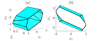
Figure 2: $(a)$ Plot of the PD-RCI set $\bm{\mathcal{S}}(\xi)$ in (7) w.r.t $\xi_{1}$ and $(b)$ projection $\bm{\mathcal{S}}(\xi)$ on $(x_{1},x_{2})$ axis.

To compare the volume gain between Problem 1 and Problem 2, we plot the volume of the set $\bm{\breve{\mathcal{S}}}$ at each iteration, as shown in Fig. 3(a). In the figure, it can be seen that there is an additional (approximately) 29% gain in the volume when the proposed Monte-Carlo based volume maximization approach is utilized.

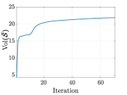
(a)

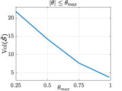
(b)

Figure 3: Volume of the set $\bm{\breve{\mathcal{S}}}$ plotted against $(a)$ iteration, $(b)$ different scheduling parameter bounds.

For comparison, we plot the computed set $\bm{\breve{\mathcal{S}}}$ and the maximal RCI set $\bm{\Omega}_{\infty}$ obtained using classical geometric approach Herceg et al. (2013) in Fig. 4. The geometric approach treats parameter as unknown bounded signals, and the control input is free from any state-feedback structure. Not surprisingly, the set $\bm{\breve{\mathcal{S}}}$ (volume $21.7907$) computed using the proposed approach was found to be larger than the maximal RCI set $\bm{\Omega}_{\infty}$ (volume $19.3703$). Moreover, the overall representational complexity of the set $\bm{\breve{\mathcal{S}}}$ is just $8$, which is exactly half the complexity of the set $\bm{\Omega}_{\infty}$, this further demonstrates the benefits of using PD-RCI sets and PDCL in the LPV setting.

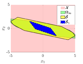
Figure 4: Admissible set $\bm{\mathcal{X}}$ (red), maximal RCI set $\bm{\Omega}_{\infty}$ (green), and RCI sets $\bm{\breve{\mathcal{S}}}$ (yellow) and $\bm{\breve{\mathcal{S}}}_{\gamma}$ (blue).

We also show the set $\bm{\breve{\mathcal{S}}}_{\gamma}$ in Fig. 4, which satisfy performance constraints $\sum_{t=0}^{\infty}x(t)^{T}Q_{x}x(t)+u(t)^{T}Q_{u}u(t)\leq\gamma$, for all $x$ within the set. Where $Q_{x}=I$, $Q_{u}=0.1$ and $\gamma=10$. Lastly, to demonstrate the main advantage of the presented algorithm, we perform an analysis in which the RCI sets are computed by changing the bound $\theta_{max}$ on the parameter $\theta$. The volume of the computed set $\bm{\breve{\mathcal{S}}}$ is plotted against parameter bound in Fig. 3(b). As expected from the theory, the volume decreases with an increase in the value of $\theta_{max}$. Nonetheless, it is interesting to observe that the proposed method is able to compute the RCI sets even for a large bound on the scheduling parameter. We remark that the geometric approach Herceg et al. (2013), failed to generate any RCI set for $\theta_{max}\geq 0.4$

7.2 Nonlinear System

One important application of the proposed approach is to compute RCI sets for nonlinear systems. For this purpose, we consider the controlled Van der Pol oscillator system in Hanema et al. (2017):

$$\dot{x}_{1}=x_{2},\,\dot{x}_{2}=-x_{1}+\mu(1-x_{1}^{2})x_{2}+u,\vspace{-0.2cm}$$ (52)

where $\mu=2$. The system should satisfy the input constraints $|u|\leq 1$ and state constraints $|x_{1}|\leq 1$, $|x_{2}|\leq 1$. For computation and simulation purpose we discretize the system using Eulers method with sampling time $0.1$ units. Further, we rewrite the system in the quasi-LPV form (5) with scheduling parameters $\xi_{1}=(2-\mu(1-x_{1}^{2}))/2$ and $\xi_{2}=\mu(1-x_{1}^{2})/2$. Using the proposed approach we compute the matrix variables defining the RCI set and the invariance inducing controller for the nonlinear system which are given as

$$[P_{1}|P_{2}] =\begin{bmatrix}\begin{array}[]{cc|cc}-0.5066&-0.1205&-0.5066&-0.1358\\ -0.4349&-0.0135&-0.4367&-0.0134\\ \;\;\,0.4238&-0.2686&\;\;\,0.4237&-0.3173\\ \;\;\,0.5280&\;\;\,0.0385&\;\;\,0.5280&\;\;\,0.0385\end{array}\end{bmatrix},$$

$$\begin{bmatrix}\!\begin{array}[]{c|c}W&\!\begin{array}[]{c}K^{1}\\ \hline\cr K^{2}\end{array}\\ \end{array}\!\!\end{bmatrix} =\begin{bmatrix}\!\!\begin{array}[]{c|c}\begin{array}[]{cc}\;\;\,0.4409&\;\;\,0.0136\\ -0.0127&\;\;\,0.1090\end{array}&\!\begin{array}[]{cc}\;\;\,0.8341&-2.3111\\ \hline\cr\;\;\,0.8727&-3.0114\end{array}\end{array}\!\!\end{bmatrix}.\vspace{-0.2cm}$$

Since the scheduling parameters $\xi_{1},\xi_{2}$ are state dependent, in accordance with Section 6.4, we compute RCI set $\bm{\breve{\mathcal{S}}}$ (46), shown in Fig. 5.

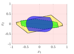
Figure 5: Admissible set $\bm{\mathcal{X}}$ (red), RCI set $\bm{\breve{\mathcal{S}}}$ (yellow; solid), RCI set using Gupta & Falcone (2019) (green; dashed) and RPI set (blue; dotted) for the Van der Pol oscillator system.

The closed-loop trajectories from all the vertices of the set $\bm{\breve{\mathcal{S}}}$ are also shown in Fig. 5. For comparison, we compute an RCI set (of a representational complexity same as $\bm{\breve{\mathcal{S}}}$) using the method presented in Gupta & Falcone (2019), which assumes the invariance inducing controller to be linear state-feedback. We show the computed set in Fig. 5 with green color. It can be seen that this set is smaller than the one generated by the proposed algorithm presented in this paper. The geometric approach Herceg et al. (2013) for computing maximal RCI set did not converge even after $24hrs$, so instead, we show a robust positive invariant (RPI) set corresponding to an LQR controller for nominal system and tuning matrices $Q=I$ and $R=1$. The representational complexity of the RPI set is $50$. Clearly, the proposed algorithm is more advantageous here since it can generate visibly larger RCI sets of low complexity.

8 Conclusion

The paper presented a novel iterative algorithm to compute a PD-RCI set and PD-invariance inducing control law for LPV systems. At each iteration of the algorithm, an SDP is solved to obtain a larger PD-RCI set successively until convergence. In the SDP, we introduced the invariance conditions, system constraints and performance constraints as LMIs, which were constructed using Finslers’s lemma and zeroth order Polya’s relaxation. Besides, we also presented a new approach for volume maximization of polytopes based on Monte-Carlo principles. It was shown that a larger invariant set could be obtained by exploiting the knowledge of parameters in the invariant set description as well as in the controller design. We assumed candidate RCI set to be 0-symmetric. This is a reasonable assumption if the system is linear and the constraints are 0-symmetric. In other cases, this assumption would be potentially conservative. Thus, a natural extension of this work could be to devise a similar algorithm for computing non-symmetrical RCI set. The authors thank Dr. Hakan Köroğlu for his valuable inputs.

Appendix A Volume maximization using Monte-Carlo integration

Based on the theory of Monte-Carlo integration Robert & Casella (2004), we present an approach which can be used to find a desirably large polytope of a predefined maximum complexity, enclosed within some known set.

Let $\bm{\mathcal{C}}$ be a set defined as,

$$\bm{\mathcal{C}}=\{x\in\mathbb{R}^{n_{x}}|Px\leq\mathbf{1}\},$$

where $P\in\mathbb{R}^{n_{p}\times n_{x}}$. We consider the following volume maximization problem,

$$\sup_{\bm{\mathcal{C}}}\int_{\bm{\mathcal{C}}}dx\quad\mathrm{s.t.}\ \ \bm{\mathcal{C}}\subseteq\bm{\mathcal{X}},$$ (53)

where $\bm{\mathcal{X}}$ is a given bounded set, not necessarily a polytope. We assume that the set containment constraints $\bm{\mathcal{C}}\subseteq\bm{\mathcal{X}}$ are already available, and are formulated as some finite-number of convex constraints (e.g., LMIs). In this section, we focus on the cost function of (53), which characterizes the volume of the polytopic set $\bm{\mathcal{C}}$. Typically, determining the exact volume $\int_{\bm{\mathcal{C}}}dx$ of a polytope $\bm{\mathcal{C}}$ is computationally challenging Bueler et al. (2000); Dyer & Frieze (1988). In our case, the problem is even more difficult as $\bm{\mathcal{C}}$ itself is not known. To this end, a procedure based on Monte-Carlo methods Robert & Casella (2004) is formulated, in order to approximate the cost in (53).

Let $\bm{\mathfrak{B}}$ be a known outer bounding box which contains the given set $\bm{\mathcal{X}}$. We generate $N$ independent random samples $\widetilde{\bm{\mathcal{X}}}=\{\widetilde{x}_{j}\}_{j=1}^{N}$, which are uniformly distributed in the given outer-bounding box $\bm{\mathfrak{B}}$.

According to Monte-Carlo integration technique, the volume of the set $\bm{\mathcal{C}}$ is approximated as,

$$\int_{\bm{\mathcal{C}}}dx\approx\frac{1}{N}\mathsf{vol}(\bm{\mathfrak{B}})\sum_{\widetilde{x}_{j}\in\widetilde{\bm{\mathcal{X}}}}\mathbb{I}_{\{\bm{\mathcal{C}}\}}(\widetilde{x}_{j}),$$ (54)

where $\mathsf{vol}(\bm{\mathfrak{B}})$ denotes the volume of the box $\bm{\mathfrak{B}}$, and $\mathbb{I}_{\{\bm{\mathcal{C}}\}}(\widetilde{x}_{j})$ is the indicator function of the set $\bm{\mathcal{C}}$ defined as,

$$\mathbb{I}_{\{\bm{\mathcal{C}}\}}(\widetilde{x}_{j})=\begin{cases}1,\ \mathrm{if}\ \ \widetilde{x}_{j}\in\bm{\mathcal{C}},\\ 0,\ \mathrm{if}\ \ \widetilde{x}_{j}\notin\bm{\mathcal{C}}.\end{cases}$$ (55)

Remark 5.

From the theory of Monte Carlo integration Robert & Casella (2004), the following limit holds with probability (w.p) $1$:

$$\lim\limits_{N\rightarrow\infty}\frac{1}{N}\mathsf{vol}(\bm{\mathfrak{B}})\sum_{\widetilde{x}_{j}\in\widetilde{\bm{\mathcal{X}}}}\mathbb{I}_{\{\bm{\mathcal{C}}\}}(\widetilde{x}_{j})=\int_{\bm{\mathcal{C}}}dx,\quad\mathrm{w.p.}1.$$

By using (54), the volume maximization problem (53) is approximated as follows,

$$\max_{\mathcal{C}}\sum_{\widetilde{x}_{j}\in\widetilde{\bm{\mathcal{X}}}}\mathbb{I}_{\{\bm{\mathcal{C}}\}}(\widetilde{x}_{j})\quad\mathrm{s.t.}\ \ \bm{\mathcal{C}}\subseteq\bm{\mathcal{X}}.$$ (56)

Note that the cost function in (56) is the sum of indicator functions $\mathbb{I}_{\{\bm{\mathcal{C}}\}}(\widetilde{x}_{j})$, which is non-convex and discontinuous. We next introduce an approximation of the cost function in order to solve (56) in a tractable manner. We approximate the discontinuous cost in (56) with a continuous-concave function such that the sample points which are contained in $\bm{\mathcal{C}}$ get the maximum cost, while the value of the cost for all $\widetilde{x}_{j}\notin\bm{\mathcal{C}}$, decreases uniformly.

For the sake of convenience, without loss of generality we modify the definition of indicator functions in the cost (56) as follows

$$\mathbb{I}_{\{\bm{\mathcal{C}}\}}(\widetilde{x}_{j})=\begin{cases}\;\;\,0,\ \ \ \mathrm{if}\,P\widetilde{x}_{j}-\mathbf{1}\leq 0,\\ -1,\ \ \mathrm{otherwise}.\end{cases}$$ (57)

Note that, this modification does not change the optimal solution of problem (56).

subsubsectionApproximation of the indicator functions

Let us first consider for each individual hyperplane $\bm{\mathcal{C}}_{i}\triangleq\{x:e^{T}_{i}(Px-\mathbf{1})\leq 0\}$ of the set $\bm{\mathcal{C}}$, the following cost $T_{\{\bm{\mathcal{C}}_{i}\}}(\widetilde{x}_{j})$,

$$T_{\{\bm{\mathcal{C}}_{i}\}}(\widetilde{x}_{j})=\begin{cases}0&\mathrm{if}\ \ e^{T}_{i}(P\widetilde{x}_{j}-\mathbf{1})\leq 0,\\ -e^{T}_{i}(P\widetilde{x}_{j}-\bm{1})&\mathrm{if}\ \ e^{T}_{i}(P\widetilde{x}_{j}-\mathbf{1})>0,\end{cases}$$ (58)

which is a piecewise linear concave approximation of the indicator functions $\mathbb{I}_{\{\bm{\mathcal{C}}_{i}\}}(\widetilde{x}_{j})$ defined for the $i$-th hyperplance of $\bm{\mathcal{C}}$. The plot of the indicator function $\mathbb{I}_{\{\bm{\mathcal{C}}_{i}\}}(\widetilde{x}_{j})$ and its approximation $T_{\{\bm{\mathcal{C}}_{i}\}}(\widetilde{x}_{j})$ is shown in Fig.6. The idea of approximating non-convex indicator function $\mathbb{I}_{\{\bm{\mathcal{C}}_{i}\}}(\widetilde{x}_{j})$ with $T_{\{\bm{\mathcal{C}}_{i}\}}(\widetilde{x}_{j})$ is similar to the relaxation of $l_{0}$-quasi-norm with $l_{1}$-norm as introduced in Benavoli & Piga (2016); Piga & Benavoli (2019) for computing outer-approximating polytopes of non-convex semialgebraic sets.

We now extend the idea of approximating the indicator functions defined for a single hyperplane $\bm{\mathcal{C}}_{i}$, to approximate the indicator function defined over the entire polytopic set $\bm{\mathcal{C}}$. In particular, we introduce the following concave function $T_{\{\bm{\mathcal{C}}\}}(\widetilde{x}_{j})$ to approximate $\mathbb{I}_{\{\bm{\mathcal{C}}\}}(\widetilde{x}_{j})$ defined in (57),

$$T_{\{\bm{\mathcal{C}}\}}(\widetilde{x}_{j})=\begin{cases}0&\!\!\!\mathrm{if}\,P\widetilde{x}_{j}\!-\!\mathbf{1}\leq 0,\\ -\left(\max\limits_{i=1,\ldots,n_{p}}e^{T}_{i}(P\widetilde{x}_{j}-\bm{1})\right)&\!\!\mathrm{otherwise}.\end{cases}$$ (59)

Note that, for the points $\widetilde{x}_{j}\notin\bm{\mathcal{C}}$, the cost $T_{\{\bm{\mathcal{C}}\}}(\widetilde{x}_{j})$ is always negative and decays uniformly in all the directions away from $\bm{\mathcal{C}}$.

Figure 6: Indicator function $\mathbb{I}_{\{\bm{\mathcal{C}}_{i}\}}(\widetilde{x}_{j})$ (blue) and its concave approximation $T_{\{\bm{\mathcal{C}}_{i}\}}(\widetilde{x}_{j})$ (red) for the $i$-th hyperplane. When $e^{T}_{i}(P\widetilde{x}_{j}-\mathbf{1})<0$, $\mathbb{I}_{\{\bm{\mathcal{C}}_{i}\}}(\widetilde{x}_{j})$ and $T_{\{\bm{\mathcal{C}}_{i}\}}(\widetilde{x}_{j})$ are overlapped and both are $0$.

Based on the approximation $T_{\{\bm{\mathcal{C}}\}}(\widetilde{x}_{j})$ in (59) of the indicator functions $\mathbb{I}_{\{\bm{\mathcal{C}}\}}(\widetilde{x}_{j})$, the problem (56) is relaxed as follows,

$$\max_{\mathcal{C}}\sum_{\widetilde{x}_{j}\in\widetilde{\bm{\mathcal{X}}}}T_{\{\bm{\mathcal{C}}\}}(\widetilde{x}_{j})\quad\mathrm{s.t.}\ \ \bm{\mathcal{C}}\subseteq\bm{\mathcal{X}}$$ (60)

Thus, by solving the constraint optimization problem (60), we try to find the matrix $P$ (defining the polytope $\bm{\mathcal{C}}$), which maximizes the number of points $\widetilde{x}_{j}$ inside the set $\bm{\mathcal{C}}$, in turn, maximizing its volume, while respecting the constraint $\bm{\mathcal{C}}\subseteq\bm{\mathcal{X}}$.

Remark 6.

With the choice of cost function $T_{\{\bm{\mathcal{C}}\}}(\widetilde{x}_{j})$ in (59), we aim at selecting the matrix $P$ of the polytope $\bm{\mathcal{C}}$, such that maximum number of points lie in the set, i.e., $\widetilde{x}_{j}\in\bm{\mathcal{C}}$. This is due to the fact that, the value of the cost $T_{\{\bm{\mathcal{C}}\}}(\widetilde{x}_{j})$ decreases linearly for the sample points $\widetilde{x}_{j}$ which lie outside the set $\bm{\mathcal{C}}$. We observe that, with this choice of the cost function, it is sufficient to select the sample points $\{\widetilde{x}_{j}\}_{j=1}^{N_{\sigma}}$ which lie on the boundary of the known outer-bounding box $\bm{\mathfrak{B}}$. This significantly reduces the computation cost to solve the optimization problem (60). Thus, in this paper, we have considered only the sample points which are on the boundary of $\bm{\mathfrak{B}}$, instead of uniformly distributed samples.

Finally, the cost function in (60) can be seen as a sum of concave functions, which can be equivalently expressed as following convex minimization problem,

$$\begin{array}[]{cc}\min&\sum_{j=1}^{N}\sigma_{j}\\ {P,\sigma_{j}}\\ \text{s.t.}&\sigma_{j}\geq 0,\ \ \forall j=1,\ldots,N\\ &P\widetilde{x}_{j}-\bm{1}\leq\sigma_{j}\bm{1},\ \ \forall j=1,\ldots,N\\ &\bm{\mathcal{C}}\subseteq\bm{\mathcal{X}},\end{array}$$ (66)

where $\sigma_{j}\in\mathbb{R}$. Thus, the final volume maximization problem consist of a linear cost and constraints, alongwith a set containment constraint.

References

- (1)
- Benavoli & Piga (2016) Benavoli, A. & Piga, D. (2016), ‘A probabilistic interpretation of set-membership filtering: Application to polynomial systems through polytopic bounding’, Automatica 70, 158 – 172.
- Blanchini & Miani (2015) Blanchini, F. & Miani, S. (2015), Set-Theoretic Methods in Control, Birkhäuser, Boston, MA.
- Blanchini et al. (2007) Blanchini, F., Miani, S. & Savorgnan, C. (2007), ‘Stability results for linear parameter varying and switching systems’, Automatica 43(10), 1817–1823.
- Blanco et al. (2010) Blanco, T. B., Cannon, M. & De Moor, B. (2010), ‘On efficient computation of low-complexity controlled invariant sets for uncertain linear systems’, International Journal of Control 83(7), 1339–1346.
- Bravo et al. (2005) Bravo, J., Limon, D., Alamo, T. & Camacho, E. (2005), ‘On the computation of invariant sets for constrained nonlinear systems: An interval arithmetic approach’, Automatica 41(9), 1583–1589.
- Bueler et al. (2000) Bueler, B., Enge, A. & Fukuda, K. (2000), Exact volume computation for polytopes: a practical study, Vol. 29, DMV SEMINAR, Springer.
- Dyer & Frieze (1988) Dyer, M. & Frieze, A. (1988), ‘On the complexity of computing the volume of a polyhedron’, SIAM Journal on Computing 17, 967–974.
- Fiacchini et al. (2010) Fiacchini, M., Alamo, T. & Camacho, E. (2010), ‘On the computation of convex robust control invariant sets for nonlinear systems’, Automatica 46(8), 1334–1338.
- Gupta & Falcone (2019) Gupta, A. & Falcone, P. (2019), ‘Full-complexity characterization of control-invariant domains for systems with uncertain parameter dependence’, IEEE Control System Letter 3(1), 19–24.
- Gupta et al. (2019) Gupta, A., Köroğlu, H. & Falcone, P. (2019), ‘Computation of low-complexity control-invariant sets for systems with uncertain parameter dependence’, Automatica 101, 330 – 337.
- Gupta et al. (2021) Gupta, A., Köroğlu, H. & Falcone, P. (2021), ‘Computation of robust control invariant sets with predefined complexity for uncertain systems’, International Journal of Robust and Nonlinear Control 31(5), 1674–1688.
- Gupta et al. (2022) Gupta, A., Mejari, M., Falcone, P. & Piga, D. (2022), ‘Computation of parameter dependent robust invariant sets for LPV models with guaranteed performance’, arXiv:2009.09778v1 .
- Hanema et al. (2017) Hanema, J., Tóth, R. & Lazar, M. (2017), Stabilizing non-linear MPC using linear parameter-varying representations, in ‘Conference on Decision and Control’, pp. 3582–3587.
- Hanema et al. (2020) Hanema, J., Tóth, R. & Lazar, M. (2020), ‘Heterogeneously parameterized tube model predictive control for LPV systems’, Automatica 111, 108622.
- Herceg et al. (2013) Herceg, M., Kvasnica, M., Jones, C. N. & Morari, M. (2013), Multi-Parametric Toolbox 3.0, in ‘European Control Conference’, Zürich, Switzerland, pp. 502–510.
- Ishihara et al. (2017) Ishihara, J. Y., Kussaba, H. T. M. & Borges, R. A. (2017), ‘Existence of continuous or constant finsler’s variables for parameter-dependent systems’, IEEE Transactions on Automatic Control 62(8), 4187–4193.
- Kothare et al. (1996) Kothare, M., Balakrishnan, V. & Morari, M. (1996), ‘Robust constrained model predictive control using linear matrix inequalities’, Automatica 32(10), 1361 – 1379.
- Liu et al. (2019) Liu, C., Tahir, F. & Jaimoukha, I. (2019), ‘Full-complexity polytopic robust control invariant sets for uncertain linear discrete-time systems’, International Journal of Robust and Nonlinear Control 29(11), 3587–3605.
- Löfberg (2004) Löfberg, J. (2004), Yalmip : A toolbox for modeling and optimization in matlab, in ‘Computer-Aided Control System Design Conference’, Taipei, Taiwan.
- Miani & Savorgnan (2005) Miani, S. & Savorgnan, C. (2005), ‘Maxis-g: a software package for computing polyhedral invariant sets for constrained LPV systems’, Conference on Decision and Control pp. 7609–7614.
- Nguyen et al. (2015) Nguyen, H., Olaru, S., Gutman, P. & Hovd, M. (2015), ‘Constrained control of uncertain, time-varying linear discrete-time systems subject to bounded disturbances’, IEEE Transactions on Automatic Control 60(3), 831–836.
- Oliveira & Peres (2005) Oliveira, R. & Peres, P. L. D. (2005), ‘Stability of polytopes of matrices via affine parameter-dependent lyapunov functions: Asymptotically exact lmi conditions’, Linear Algebra and its Applications 405, 209 – 228.
- Piga & Benavoli (2019) Piga, D. & Benavoli, A. (2019), Semialgebraic outer approximations for set-valued nonlinear filtering, in ‘18th European Control Conference (ECC)’, Naples, Italy, pp. 400–405.
- Pólik & Terlaky (2007) Pólik, I. & Terlaky, T. (2007), ‘A survey of the s-lemma’, SIAM Review 49(3), 371–418.
- Raković & Baric (2010) Raković, S. V. & Baric, M. (2010), ‘Parameterized Robust Control Invariant Sets for Linear Systems: Theoretical Advances and Computational Remarks’, IEEE Transactions on Automatic Control 55(7), 1599–1614.
- Robert & Casella (2004) Robert, C. & Casella, G. (2004), Monte Carlo statistical methods, Springer Science.