TreeCaps: Tree-Based Capsule Networks for Source Code Processing

Abstract

Recently program learning techniques have been proposed to process source code based on syntactical structures (e.g., Abstract Syntax Trees) and/or semantic information (e.g., Dependency Graphs). While graphs may be better at capturing various viewpoints of code semantics than trees, constructing graph inputs from code need static code semantic analysis that may not be accurate and introduces noise during learning. On the other hand, syntax trees are precisely defined according to the language grammar and easier to construct and process than graphs. We propose a new tree-based learning technique, named TreeCaps, by fusing capsule networks with tree-based convolutional neural networks, to achieve learning accuracy higher than existing graph-based techniques while it is based only on trees. TreeCaps introduces novel variable-to-static routing algorithms into the capsule networks to compensate for the loss of previous routing algorithms. Aside from accuracy, we also find that TreeCaps is the most robust to withstand those semantic-preserving program transformations that change code syntax without modifying the semantics. Evaluated on a large number of Java and C/C++ programs, TreeCaps models outperform prior deep learning models of program source code, in terms of both accuracy and robustness for program comprehension tasks such as code functionality classification and function name prediction. The implementation of TreeCaps is publicly available at https://github.com/bdqnghi/treecaps.

Introduction

Software developers often spend the majority of their time in navigating existing program code bases to understand the functionality of existing source code before implementing new features or fixing bugs (Xia et al. 2018; Evans Data Corporation 2019; Britton et al. 2012). Learning a model of programs has been found useful for their tasks such as classifying the functionality of programs (Nix and Zhang 2017; Dahl et al. 2013; Pascanu et al. 2015; Rastogi, Chen, and Jiang 2013), predicting bugs (Yang et al. 2015; Li et al. 2017, 2018; Zhou et al. 2019), translating programs (Chen, Liu, and Song 2018; Gu et al. 2017; Bui, Jiang, and Yu 2018; Bui, Yu, and Jiang 2019; Nghi, Yu, and Jiang 2019), etc.

It is common that adding semantic descriptions (e.g., via code comments, visualizing code control flow graphs, etc.) may enhance human understanding of programs and ease machine learning. With the help of static code dependency analysis techniques (Nielson, Nielson, and Hankin 1999), for example, Gated Graph Neural Networks (GGNN) (Li et al. 2016; Fernandes, Allamanis, and Brockschmidt 2019; Allamanis, Brockschmidt, and Khademi 2018) learn code semantics via graphs where edges are added between the code syntax tree nodes to indicate various kinds of dependencies between the nodes. However, adding such edges requires extra processing of ASTs and may introduce noise for different learning tasks since there is no consensus on which types of edges are needed for which tasks.

There also exist deep learning techniques that process code syntax trees or abstract syntax trees (ASTs) (Mou et al. 2016; Alon et al. 2019b; Zhang et al. 2019). However, they are limited in how they represent and learn ASTs although ASTs entail all code semantics. Tree-Based Convolutional Neural Network (TBCNN) (Mou et al. 2016) shares the same computational principle as GGNN, i.e., information is accumulated from nearby children to parent nodes only, which limits the number of iterations for a node to accumulate information from its distant descendants. Code2vec (Alon et al. 2019b) decomposes trees into a bag of path-contexts for learning; ASTNN (Zhang et al. 2019) splits big trees for programs and functions into smaller subtrees for individual statements. They adapt recurrent neural network models to learn the path-contexts or flattened subtrees, but still likely miss code dependency information that is not represented in the decomposed paths and subtrees.

It is desirable to learn code models via ASTs because trees can be more efficiently and precisely constructed from code than graphs without the need of semantic analysis that may be expensive or inaccurate. Towards this goal, this paper proposes a novel architecture called TreeCaps by fusing capsule networks (Sabour, Frosst, and Hinton 2017) with TBCNN to build code models from trees, as a complement to graph-based models. TreeCaps first adapts TBCNN to take in trees and extract (local) node features with its convolution capability and converts the node features into capsules in its Primary Variable Capsule (PVC) layer where the number of capsules can change for different tree inputs. It then adapts CapsNet by introducing two methods to route the dynamic number of capsules in PVC to a static number of capsules in its Secondary Capsule (SC) layer. Our first method inherits the dynamic routing algorithm (Sabour, Frosst, and Hinton 2017) for static numbers of capsules; it shares a global transformation matrix across every pair of capsules between the layers (Yang et al. 2018; Zhang and Chen 2019). Our second method is a novel Variable-to-Static (VTS) routing algorithm that selects the capsules with the most prominent outputs in the PVC layer and squeezes them into a fixed set of capsules. The method utilizes the common intuition that code semantics can often be determined by considering only a portion of code elements. Further, we apply a dynamic routing algorithm from the capsules in the SC layer to the final Code Capsule (CC) layer whose number of capsules is fixed according to a specific learning task, to get the vector embeddings of the trees for the task. Compared to the max-pooling method to combine node features in TBCNN, the pipeline of our routing methods (PVC $\rightarrow$ SC $\rightarrow$ CC) can learn more complex combinations of AST features.

Across codebases in C/C++ and Java with respect to commonly compared program comprehension tasks such as code functionality classification and function name prediction, our empirical evaluation shows that TreeCaps achieves better classification accuracy and better F1 score in prediction compared to other code learning techniques such as Code2vec, Code2seq, ASTNN, TBCNN, GGNN, GREAT and GNN-FiLM. We have also applied three types of semantic-preserving transformations (Rabin et al. 2020; Zhang et al. 2020; Wang and Su 2019) that transform programs into syntactically different but semantically equivalent code to attack the models. Evaluations also show that our TreeCaps models are the most robust, able to preserve its predictions for transformed programs more than other learning techniques.

Related Work

There has been huge interest in applying deep learning techniques for software engineering tasks such as program functionality classification (Mou et al. 2016; Zhang et al. 2019), function name prediction (Fernandes, Allamanis, and Brockschmidt 2019), bug localization (Pradel and Sen 2018; Gupta, Kanade, and Shevade 2019), code clone detection (Zhang et al. 2019), program refactoring (Hu et al. 2018), program translation (Chen, Liu, and Song 2018), and code synthesis (Brockschmidt et al. 2019). A model of source code can often be learned in two steps: (1) convert source code into suitable intermediate representations, and (2) design learning networks to process the representations.

Mou et al. (2016) parse code into ASTs and design Tree-Based Convolutional Neural Networks (TBCNNs) as the learning networks. Allamanis, Brockschmidt, and Khademi (2018) extend ASTs to graphs by adding a variety of code dependencies as edges among tree nodes, intended to represent code semantics, and apply Gated Graph Neural Networks (GGNN) (Li et al. 2016) to learn the graphs, which indeed enhances the performance of TBCNN (Mou et al. 2016) for certain tasks. GNN-FiLM (Brockschmidt 2019) is also a graph-based model that explores by applying feature-wise linear modulation (FiLM) on Graph Neural Network (GNN). Hellendoorn et al. (2019) proposes a hybrid approach to combine sequence-based models (Recurrent Neural Networks, Transformer) and graph-based models (GNNs) into a model called Graph Relational Embedding Attention Transformer (GREAT) to address the major drawback of GGNN that can only capture local information of the source code. While the graph-based model extracts local features of source code, the sequence-based model captures global features, their combination improves the performance of GREAT over GNNs.

Code2vec (Alon et al. 2019b), Code2seq (Alon et al. 2019a), and ASTNN (Zhang et al. 2019) are designed based on splitting ASTs into smaller ones, either as a bag of path-contexts or as flattened subtrees representing individual statements, and use various kinds of Recurrent Neural Network (RNN) to learn such code representations. Inst2vec (Ben-Nun, Jakobovits, and Hoefler 2018) uses the RNN to model the Intermediate Representation of the binary code that is independent of the source programming language.

Capsule networks (CapsNet) (Sabour, Frosst, and Hinton 2017; Hinton, Sabour, and Frosst 2018) use dynamic routing to model spatial and hierarchical relations among objects in an image. The techniques have been successfully applied to image processing tasks such as image classification, character recognition, and text classification (Jayasundara et al. 2019; Rajasegaran et al. 2019; Yang et al. 2018; Li et al. 2019). However, none of the studies has considered complex tree data as input, which is however natural for programs. Capsule Graph Neural Networks (Zhang and Chen 2019) proposed to classify biological and social network graphs does not handle tree- or graph-based code syntax. To the best of our knowledge, we are the first to adapt capsule networks for program source code processing to learn code models on syntax trees directly, without the need for extra static program semantic analysis techniques that may be expensive or introduce inaccuracies (Nielson, Nielson, and Hankin 1999).

Tree-based Capsule Networks

An overview of the TreeCaps architecture is shown in Fig. 1.

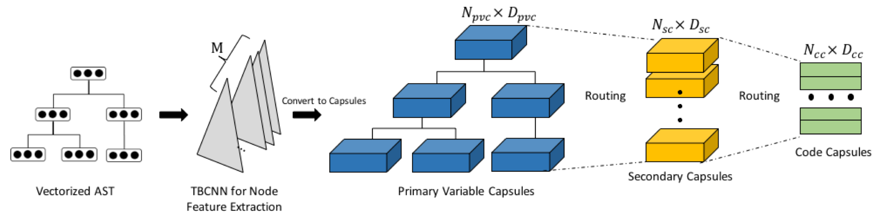
Figure 1: Source codes are parsed, vectorized and fed into the TBCNN to extract node features, then the node features are combined through the TreeCaps network.

The steps of our technique are as follows:

• The code snippet in the training data is parsed into an AST and vectorized. The node vectors are fed into the TBCNN to extract node features.

• The node features will be used as the input for the Primary Variable Capsule (PVC) layer to group the tensor outputs of the TBCNN layers into a set of capsules. The number of capsules in this layer is dynamic

• The capsules in the PVC layer are then routed and reduced to a fixed number of capsules in the Secondary Capsule (SC) layer. The SC layer is to combine the capsules in the PVC layer into a new set of capsules, in which the number of capsules in this layer is static.

• The outputs of the SC layer are routed to the final Code Capsule (CC) layer where capsules can be seen as the vector representations for the input code, and can be trained with respect to various code comprehension tasks, such as code functionality classification and function name prediction.

Tree-based Convolutional Neural Networks

We briefly introduce the Tree-based Convolutional Neural Networks (TBCNN, (Mou et al. 2016)) for processing tree-structured inputs used in TreeCaps.

A tree $T=(V,E,X)$ consists of a set of nodes $V$, a set of node features $X$, and a set of edges $E$. An edge in a tree connects a node and its children. Each node in an AST also contains its corresponding texts (or tokens) and its type (e.g., operator types, statement types, function types, etc.) from the underlying code. Initially, we annotate each node $v\in V$ with a $D$-dimensional real-valued vector $x_{v}\in\mathbb{R}^{D}$ representing the features of the node. We associate every node $v$ with a hidden state vector $h_{v}$, initialized from the feature embedding $x_{v}$, which can be computed from a simple concatenation of the embeddings of its texts and type (Allamanis, Brockschmidt, and Khademi 2018). The embedding matrices for the texts and types can be learned in the whole model training pipeline.

In TBCNN, a convolution window over an AST is emulated via a binary tree, where the weight matrix for each node is a weighted sum of three fixed matrices $\mathbf{W}^{t}$, $\mathbf{W}^{l}$, $\mathbf{W}^{r}\in\mathbb{R}^{D\times D}$ (for the “top”, “left”, and “right” node respectively) and a bias term $\mathbf{b}\in\mathbb{R}^{D}$. Hence, for a convolution window of depth $d$ in the original AST containing $K=2^{d}-1$ nodes (including the parent node) with vectors $[\mathbf{x}_{1},...,\mathbf{x}_{K}]$, where $\mathbf{x_{i}}\in\mathbb{R}^{D}$, the convolutional output $\mathbf{y}$ of the window is defined as follows:

$$\mathbf{y}=tanh(\sum_{i=1}^{K}[\eta_{i}^{t}\mathbf{W}^{t}+\eta_{i}^{l}\mathbf{W}^{l}+\eta^{r}_{i}\mathbf{W}^{r}]\mathbf{x}_{i}+\mathbf{b}),$$ (1)

where $\eta_{i}^{t},\eta_{i}^{l},\eta_{i}^{r}$ are weights calculated corresponding to the depth and the position of the nodes. One can see this as a way to learn the position of a node inside a tree. A TBCNN model usually stacks $m$ such convolutional layers together to generate the final node embeddings, where the output at layer $m$ will be used as the input for the next, i.e. the $m+1$-th layer. Each layer has its own $\mathbf{W}^{t}$, $\mathbf{W}^{l}$, $\mathbf{W}^{r}\in\mathbb{R}^{D\times D}$ and the bias term $\mathbf{b}\in\mathbb{R}^{D}$ with different initialization.

The Primary Variable Capsule Layer (PVC)

The PVC layer is to group the outputs of the convolutional layers into the set of capsules for the routing purpose. Each convolutional layer will output a tensor with shape $|V|\times D$, where $|V|$ is the number of nodes in the AST, $D$ is the dimension size of the node embedding. There are m such TBCNN layers; then the outputs of such m layers will be a tensor with shape $|V|\times D\times m$. We set $N_{pvc}=|V|\times D$, $D_{pvc}=m$ so that the PVC layer will receive the input of the shape $(N_{pvc}\times D_{pvc})$. It will go through a non-linear squash function (Sabour, Frosst, and Hinton 2017) and get the output with the same shape $(N_{pvc}\times D_{pvc})$. Each output capsule $\mathbf{u}_{i}$ from the squash function represents the probability of existence of an entity by the vector length, formally defined as:

$$\mathbf{u}_{i}=\frac{||\mathbf{c}_{i}||^{2}}{||\mathbf{c}_{i}||^{2}+1}\cdot\frac{\mathbf{c}_{i}}{||\mathbf{c}_{i}||}.$$ (2)

Hence, the output of the PVC layer is $\mathbf{X_{pvc}}\in\mathbb{R}^{N_{pvc}\times D_{pvc}}$.

The Secondary Capsule Layer (SC)

Because $N_{pvc}$ is dynamic as $|V|$ is dynamic, one can not route the output of the PVC layer directly into the final capsule layer (similar to  Sabour, Frosst, and Hinton (2017). To address this, we propose 2 methods to combine the dynamic number of capsules in PVC into static number of capsules in an intermediate layer, called the Secondary Capsule layer.

Sharing Weights across Child Capsules with Dynamic Routing (DRSW)

To combine the capsules in layer $l$ into layer $l+1$, the key is to define a set of transformation matrices. Each matrix is multiplied with each of the capsule in layer $l$ ( Sabour, Frosst, and Hinton (2017)). In this way, the matrices will be learned as parameters through the end-to-end learning process so the capsules in layer $l$ will be combined through matrices into the capsules in layer $l+1$. Since the number of capsules in the PVC is dynamic, a global transformation matrix cannot be defined in practice with variable dimensions. The solution for this problem is to defined a shared transformation matrix $\mathbf{W_{s}}\in\mathbb{R}^{N_{pvc}\times D_{pvc}\times D_{sc}}$ across the child capsules, where $N_{pvc}$ is the number of capsules in the PVC layer (Yang et al. 2018), $D_{sc}$ is the dimension of the capsules in the SC layer, and a dynamic algorithm routes the capsules (as summarized in Algo.1).

In Algo.1, for each capsule $i$ in the $l$-th PVC layer and each capsule $j$ in the $l+1$-th SC layer, we multiply the output of the PVC layer $\mathbf{u}_{i}$ by the shared transformation matrix $\mathbf{W}_{s}$ to produce the prediction vectors $\mathbf{\hat{u}}_{j|i}=\mathbf{W}_{s}\mathbf{u}_{i}$. The “prediction vectors” are responsible for predicting the strength of each capsule in the PVC layer, then a weighted sum over all “prediction vectors” $\mathbf{\hat{u}}_{j|i}$ will produce the capsule $j$ in the SC layer. The trainable shared transformation matrix learns the part-whole relationships between the primary capsules and secondary capsules, while effectively transforms $\mathbf{u}_{i}$’s into the same dimensionality as $\mathbf{v}_{j}$ where each $\mathbf{v}_{j}$ denotes the capsule output of the SC layer. The coupling coefficients $\beta_{ij}$ between capsule $i$ and all the capsules in the SC layer sum to 1 and are determined by a “routing softmax” whose initial logits $\alpha_{ij}$ are the log prior probabilities that capsule $i$ in PVC layer should be coupled to capsule $j$ in the SC layer. Then we use $r$ iterations to refine $\beta_{ij}$ based on the agreements between the prediction vectors $\mathbf{\hat{u}}_{j|i}$ and the secondary capsule outputs $\mathbf{v}_{j}$ where $\mathbf{v}_{j}=squash(\sum_{i}\beta_{ij}\mathbf{\hat{u}}_{j|i})$.

Algorithm 1 Dynamic Routing

1:procedure Routing($\mathbf{\hat{u}}_{j|i},r,l$)

2:     Initialize $\forall i\in[1,l],\forall j\in[1,l+1],\alpha_{ij}\leftarrow 0$

3:     for r iterations do

4:         $\forall i\in[1,l],\mathbf{\beta}_{i}\leftarrow softmax(\mathbf{\alpha}_{i})$

5:         $\forall j\in[1,l+1],\mathbf{v}_{j}\leftarrow squash(\sum_{i}\beta_{ij}\mathbf{\hat{u}}_{j|i})$

6:         $\forall i\in[1,l],\forall j\in[1,l+1],\alpha_{ij}\leftarrow\alpha_{ij}+\mathbf{\hat{u}}_{j|i}\cdot\mathbf{v}_{j}$

7:     end for

8:     return $\mathbf{v}_{j}$

9:end procedure

Variable-to-Static Routing (VTS)

Sharing the transformation matrix reduces the ability to learn different features because each pair of capsules is supposed to have its transformation matrix. Due to this limitation, we offer the second solution to route the variable number of capsules in the PVC layer. It is based on an observation of source code that, in practice, not every node of the AST contributes towards a source code learning task. Often, source code consists of non-essential entities, and only a portion of all entities determine the code class. Therefore, we propose a novel variable-to-static capsule routing algorithm, summarized in Algo. 2. The intuition of this algorithm is that we squeeze the variable number of capsules in the PVC layer to a static number of capsules by choosing only the most important capsules in the PVC layer. The major difference between the VTS algorithm and the DRSW algorithm is that the DRSW needs to produce prediction vectors by multiplying the capsule outputs in PVC layer with the shared transformation matrix, and then the prediction vectors will be combined to produce the capsules for SC layer; whereas in the VTS, the capsule outputs in the PVC layer are selected and the prominent ones are used to initialize the capsules in SC layer directly.

Algorithm 2 Variable-to-Static Capsule Routing

1:procedure Routing($\mathbf{u}_{i},r,a,b$)

2:     $\mathbf{U_{sorted}}\leftarrow sort([\mathbf{u}_{1},...,\mathbf{u}_{b}])$

3:     Initialize $\mathbf{v}_{j}$ : $\forall i,j\leq a,\mathbf{v_{j}\leftarrow U_{sorted}}[i]$

4:     Initialize $\alpha_{ij}$ : $\forall j\in[1,a],\forall i\in[1,b],\alpha_{ij}\leftarrow 0$

5:     for $r$ iterations do

6:         $\forall j\in[1,a],\forall i\in[1,b],f_{ij}\leftarrow\mathbf{u}_{i}\cdot\mathbf{v}_{j}$

7:         $\forall j\in[1,a],\forall i\in[1,b],\alpha_{ij}\leftarrow\alpha_{ij}+f_{ij}$

8:         $\forall i\in[1,b],\bm{\beta}_{i}\leftarrow Softmax(\bm{\alpha}_{i})$

9:         $\forall j\in[1,a],\mathbf{v}_{j}\leftarrow Squash(\sum_{i}$$\beta_{ij}\mathbf{u}_{i})$

10:     end for

11:     return $\mathbf{v}_{j}$

12:end procedure

We initialize the outputs of the SC layer with the outputs of the $a$ capsules with the highest $L_{2}$ norms in the PVC layer. Hence, the outputs of the PVC layer, $[\mathbf{u}_{1},...,\mathbf{u}_{N_{pvc}}]$, are first ordered by their $L_{2}$ norms to obtain $\mathbf{U_{sorted}}$, and then the first $a$ vectors of $\mathbf{U_{sorted}}$ are assigned as $\mathbf{v}_{j},j\leq a$.

Since the probability of the existence of an entity is denoted by the length of the capsule output vector ($L_{2}$ norm), we only consider the entities with the highest existence probabilities for initialization (in other words, highest activation) following the aforementioned intuition. It should be noted that the capsules with the $a$-highest norms are used only for the initialization; the actual outputs of the static capsules in the SC layer are determined by iterative runs of the variable-to-static routing algorithm. It is the capsules with the most prominent outputs along with the capsules of the highest vector similarities to them that get routed to the next layer. In this way, rare capsules, when they have prominent outputs, are still preserved and routed to the next layer.

Next, we route all $b$ capsules in the PVC layer based on the similarity among them and the static capsule layer outputs. We initialize the routing coefficients as $\alpha_{ij}=0$, equally to the $b$ capsules in the PVC layer. Subsequently, they are iteratively refined based on the agreement between the current SC layer outputs $\mathbf{v}_{j}$ and the PVC layer outputs $\mathbf{u}_{i}$. The agreement, in this case, is measured by the dot product, $f_{ij}\leftarrow\mathbf{u}_{i}\cdot\mathbf{v}_{j}$, and the routing coefficients are adjusted with $f_{ij}$ accordingly. If a capsule $u$ in the PVC layer has a strong agreement with a capsule $j$ in the SC layer, then $f_{ij}$ will be positively large; whereas if there is strong disagreement, then $f_{ij}$ will be negatively large. Subsequently, the sum of vectors $\mathbf{u}_{i}$ is weighted by the updated $\beta_{ij}$ to calculate $\mathbf{s}_{j}$, which is then squashed to update $\mathbf{v}_{j}$.

The Code Capsules Layer (CC)

The CC layer outputs the vector embeddings for the code $\mathbf{X_{cc}}\in\mathbb{R}^{N_{cc}\times D_{cc}}$, where $D_{cc}$ is the dimensionality of each code capsule and $N_{cc}$ is fixed with respect to a specific code learning task. Note in the outputs of the SC layer $\mathbf{X_{sc}}\in\mathbb{R}^{N_{sc}\times D_{sc}}$, $N_{sc}$ is also fixed,

The following subsections explain how we set $N_{cc}$ and train the TreeCaps models for different code learning tasks.

Code (Functionality) Classification

This task is to, given a piece of code, classify the functionality class it belongs to. We want $N_{cc}$ capsules in the CC layer, each of which corresponds to a functionality class of code that appeared in the training data. As such, we let $N{cc}=\kappa$, where $\kappa$ is the number of functionality classes. We calculate the probability of the existence of each class by obtaining $L_{2}$ norm of each capsule output vector. We use the margin loss (Sabour, Frosst, and Hinton 2017) as the loss function during training.

Function (Method) Name Prediction

This task is to, given a piece of code (without its function header), predict a meaningful name that reflects the functionality of the code. For this task, following Alon et al. (2019b)’s prediction approach, we let $N_{cc}$ of the CC layer be $1$, and the output of the only capsule represent the vector for the given piece of code. In this case, the output capsules of the CC layer has the shape of $\mathbf{X_{cc}}\in\mathbb{R}^{1\times D_{cc}}$, which is also the code vector that represents for the code snippet $\bm{C}$, denoted as $\bm{v_{C}}$. The vector embeddings of the function are learn-able parameters, formally defined as $functions\_vocab\in\mathbb{R}^{\left|L\right|\times D_{cc}}$, where $L$ is the set of function names found in the training corpus. The embedding of $function_{i}$ is row $i$ of $functions\_vocab$. The predicted distribution of the model $q\left(l\right)$ is computed as the (softmax-normalized) dot product between the context vector $\bm{v_{C}}$ and each of the function embeddings:

$$for\,l_{i}\in L:\,q\left(l_{i}\right)=\frac{\exp(\bm{v_{C}}^{T}\cdot functions\_vocab_{i})}{\sum_{l_{j}\in L}\exp(\bm{v_{C}}^{T}\cdot functions\_vocab_{j})}$$ (3)

where $q\left(l_{i}\right)$ is the normalized dot product between the vector of $l_{i}$ and the code vector $\bm{v_{C}}$, i.e., the probability that a function name $l_{i}$ should be assigned to the given code snippet $\bm{C}$. We choose $l$ that gives the maximum probability for the snippet $\bm{v_{C}}$. For training the network, we use cross-entropy as the loss function.

Empirical Evaluation

General Settings.

We use fAST, an efficient parser (Yu 2019) to parse code into ASTs in a binary format equivalent to SrcML (Collard, Decker, and Maletic 2013); we also use another parser PycParser used by TBCNN and ASTNN for a fairer comparison and evaluate the effects of parser choices. For the parameters in our TBCNN layer, we follow Mou et al. (2016) to set the size of type embeddings to 128, the size of text embeddings to 128, and the number of convolutional steps $m$ to 8. For the capsule layers, we set $N_{sc}=100$, $D_{sc}=16$, $D_{cc}=16$ and routing iterations $r$ = 3. We use Tensorflow libraries to implement TreeCaps. To train the models, we use the Rectified Adam (RAdam) optimizer (Liu et al. 2019) with an initial learning rate of $0.001$ subjected to decay on an Nvidia Tesla P100 GPU.

Baselines

We choose a few recent code modeling techniques to compare with TreeCaps: Code2vec (Alon et al. 2019b), Code2seq (Alon et al. 2019a), TBCNN (Mou et al. 2016), ASTNN (Zhang et al. 2019), GGNN (Allamanis, Brockschmidt, and Khademi 2018), GREAT (Hellendoorn et al. 2019). We also include a token-based baseline by treating source code as sequences of tokens and using a neural machine translation (NMT) baseline, which is a 2-layer Bi-LSTM, to process the token sequences. A common setting used among all these techniques is that they all utilize both node type and token information to initialize a node in ASTs. We set both the dimensionality of type embeddings and text embeddings to 128. Note that we try our best to make the baselines as strong as possible by choosing the hyper-parameters above as the “optimal settings” according to their papers or code.

We use different baselines for the two tasks since not all the models were designed for both tasks. For the graph-based models (GGNN, GREAT), there is no publicly available tool to generate the needed graph representations of code by adding semantic edges into the ASTs as presented in (Allamanis, Brockschmidt, and Khademi 2018), so we have implemented a tool by ourselves to represent the code as graphs with the assistance of SrcSlice and SrcML. We include as many edges presented in (Allamanis, Brockschmidt, and Khademi 2018) as possible to ensure the graph-based baselines are strong. The set of edges we used are: parent_child, next_token, last_lexical_use, last_write, return_to, compute_from, guarded_by, guarded_by_negation. We also add the backward edges for these edge types. For Code2vec, we follow the settings suggested in their latest Code2seq paper as well as the implementation in the official software artifacts to reproduce their results.

Setups for Code Classification

Datasets, Metrics, and Models.

We use datasets in two different programming languages. The first Sorting Algorithms (SA) dataset is from Nghi, Yu, and Jiang (2019), which contains 10 algorithm classes of 1000 sorting programs written in Java. The second OJ dataset is from Mou et al. (2016), which contains 52000 C programs of 104 classes. We split each dataset into training, testing, and validation sets by the ratios of 70/20/10. We use the same classification accuracy metric as Mou et al. (2016) for comparing classification results.

We compare TreeCaps with other techniques that have been applied to the code classification task, such as TBCNN (Mou et al. 2016), ASTNN (Zhang et al. 2019), Code2vec (Alon et al. 2019b), GGNNs (Allamanis, Brockschmidt, and Khademi 2018; Fernandes, Allamanis, and Brockschmidt 2019). Since TBCNN (Mou et al. 2016) and ASTNN (Zhang et al. 2019) use PycParser to parse code into AST, we also compare TreeCaps with all the baselines by using both PycParser and SrcML. We also include an ablation study to measure the impact of different combinations of node initialization and representation.

Table 1: Performance in Code Functionality Classification compared. A ‘-’ means that the model is not suited to use the relevant node representation or the parser and thus not evaluated.

Model	SA Dataset (1000 samples)			OJ Dataset (52000 samples)
Parser	SrcML			PycParser			SrcML
Initial Info	Type	Token	Combine	Type	Token	Combine	Type	Token	Combine
2-layer Bi-LSTM	-	81.83	-	-	83.51	-	-	83.51	-
Code2vec	-	-	80.44	-	-	86.21	-	-	80.15
TBCNN	78.09	71.23	82.02	92.64	87.97	95.21	81.15	71.15	83.90
ASTNN	-	-	84.32	-	-	98.2	-	-	85.32
GGNN	82.12	74.25	83.81	-	-	-	85.23	72.23	85.89
Treecaps-DRSW	83.15	74.56	84.57	94.75	89.42	96.74	83.59	77.59	87.77
Treecaps-VTS	84.60	78.15	85.43	95.88	90.21	98.32	83.40	79.56	88.40

Code Classification Results.

As shown in Table 1, TreeCaps models, especially TreeCaps-VTS, have the highest classification accuracy when combining node type and node token information, for both of the SA and OJ datasets. When only node token information is used, the simpler 2-layer Bi-LSTM models may achieve higher accuracy. The OJ dataset also shows that the choice of a parser affects the performance significantly. The models using PycParser all achieve higher accuracy than the models using SrcML. This is due to the reason that ASTs generated by PycPaser have only around 50 node types, while SrcML has more than 400 node types, which makes it harder for the networks to learn. Across the datasets, The TreeCaps-VTS performs consistently the best in terms of the F1 measure among the baselines under different settings.

Setups for Function Name Prediction

Datasets, Metrics, and Models.

We use the datasets from Code2seq(Alon et al. 2019a) containing three sets of Java programs: Java-Small (700k samples), Java-Med (4M samples), and Java-Large(16M samples). These datasets have been split into training/testing/validation by projects. We measure prediction performance using precision (P), recall (R), and F1 scores over the sub-words in generated names, following the metrics used by Alon et al. (2019b); Fernandes, Allamanis, and Brockschmidt (2019). For example, a predicted name result_compute is considered to be an exact match of the actual name computeResult; predicted compute has full precision but only 50% recall; and predicted compute_model_result has full recall but only 67% precision.

We use these baselines for the function name prediction task: Code2vec, TBCNN, Code2seq, GGNN, the 2-layer Bi-LSTM, and and GREAT (Hellendoorn et al. 2019), a hybrid model mixing sequence-based and graph-based techniques. The inputs for GREAT is graph representations of code, similar to GGNN, and we have adapted this baseline into the function name prediction task. We train each of the models for 50 epochs for each of the three datasets. We also measure the training time for each of the models.

Function Name Prediction Results.

As shown in Table 2, TreeCaps-VTS outperforms all other baselines for most of the settings. TreeCaps-DRSW also performs well but still worse than TreeCaps-VTS. Both TreeCaps-VTS and TreeCaps-DRSW are better than the graph-based models (GGNN, GREAT) and path-based model (Code2seq, Code2vec) without the need for additional code dependency analysis for constructing graphs. Regarding the training time, GGNN is the longest. The training time of both TreeCaps models is comparable to GREAT, the state-of-the-art graph-based technique to model source code, while TreeCaps-VTS is slightly faster.

Table 2: Performance of TreeCaps and the baselines for Function (Method) Name Prediction

Model	java-small (700k Samples)				java-med (4M Samples)				java-large (16M Samples)
Metric	P	R	F1	Training Time	P	R	F1	Training Time	P	R	F1	Training Time
2-layer Bi-LSTM	40.02	31.84	35.46	26.3h	49.73	40.12	44.82	65.2h	56.56	49.27	52.63	150h
TBCNN	40.89	27.67	32.24	20.6h	45.23	41.41	43.23	58.7h	58.15	40.91	49.40	165h
Code2vec	23.35	22.01	21.36	47.9h	36.43	27.93	31.89	91.6h	44.24	38.25	41.56	222h
Code2seq	50.42	35.43	42.56	56.3h	62.56	46.83	53.66	100h	63.25	54.03	58.96	235h
GGNN	40.25	35.25	36.86	75.8h	50.14	41.25	45.31	142h	50.18	44.25	46.23	280h
GREAT	47.25	39.97	43.56	55.5h	57.15	44.12	51.42	110h	61.35	55.86	58.25	205h
TreeCaps-DRSW	45.19	39.49	42.89	61.5h	60.19	41.15	52.56	125h	59.41	52.93	57.82	153h
TreeCaps-VTS	52.62	41.36	46.78	45.1h	64.38	48.87	55.67	105h	66.85	56.32	61.34	180h

Model Analysis

Table 3: Model robustness, measured as percentage of predictions changed wrt. semantic-preserving program transformations. The lower the more robust.

Model	VR	US	PS	Average
Code2vec	22.45%	19.42%	26.56%	22.81%
Code2seq	16.84%	21.82%	20.12%	19.59%
TBCNN	11.16%	19.36%	21.67%	17.39%
GGNN	15.34%	18.89%	16.42%	16.88%
GREAT	13.48%	17.75%	16.51%	15.90%
TreeCaps-DRSW	11.23%	15.76%	16.54%	14.51%
TreeCaps-VTS	9.53%	14.08%	13.87%	12.49%

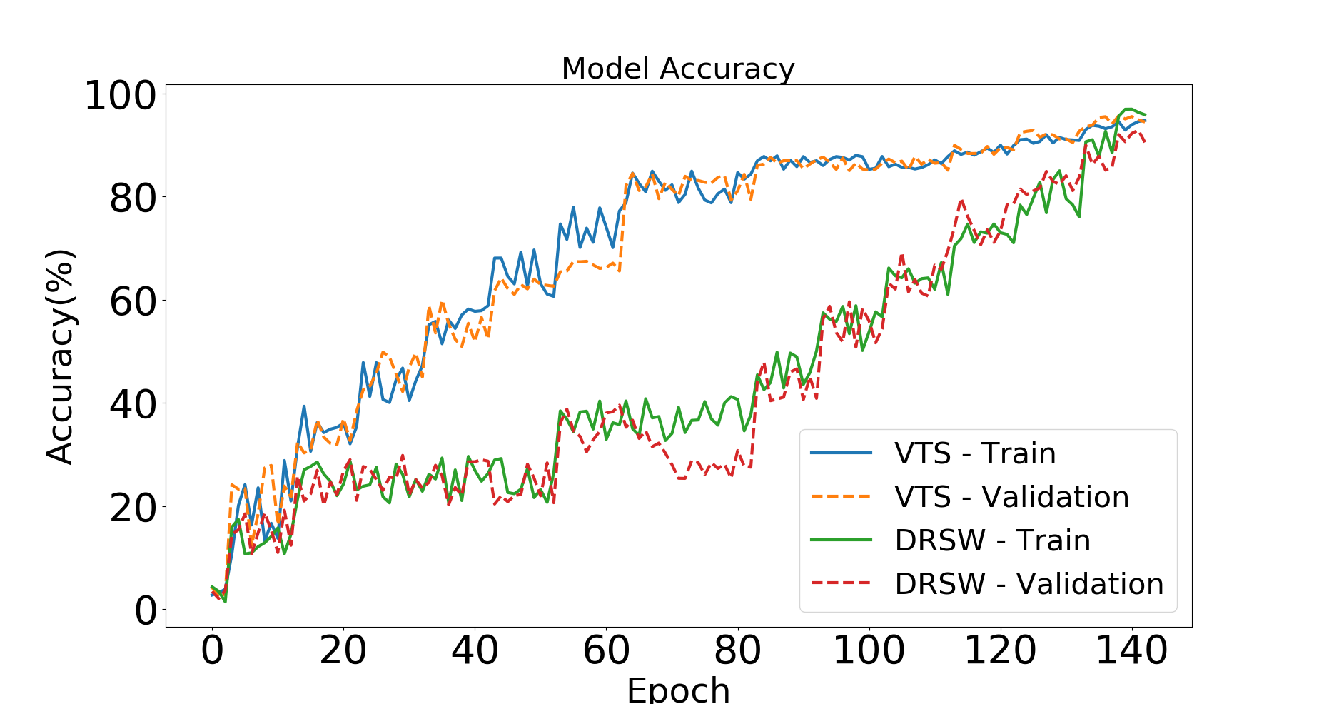
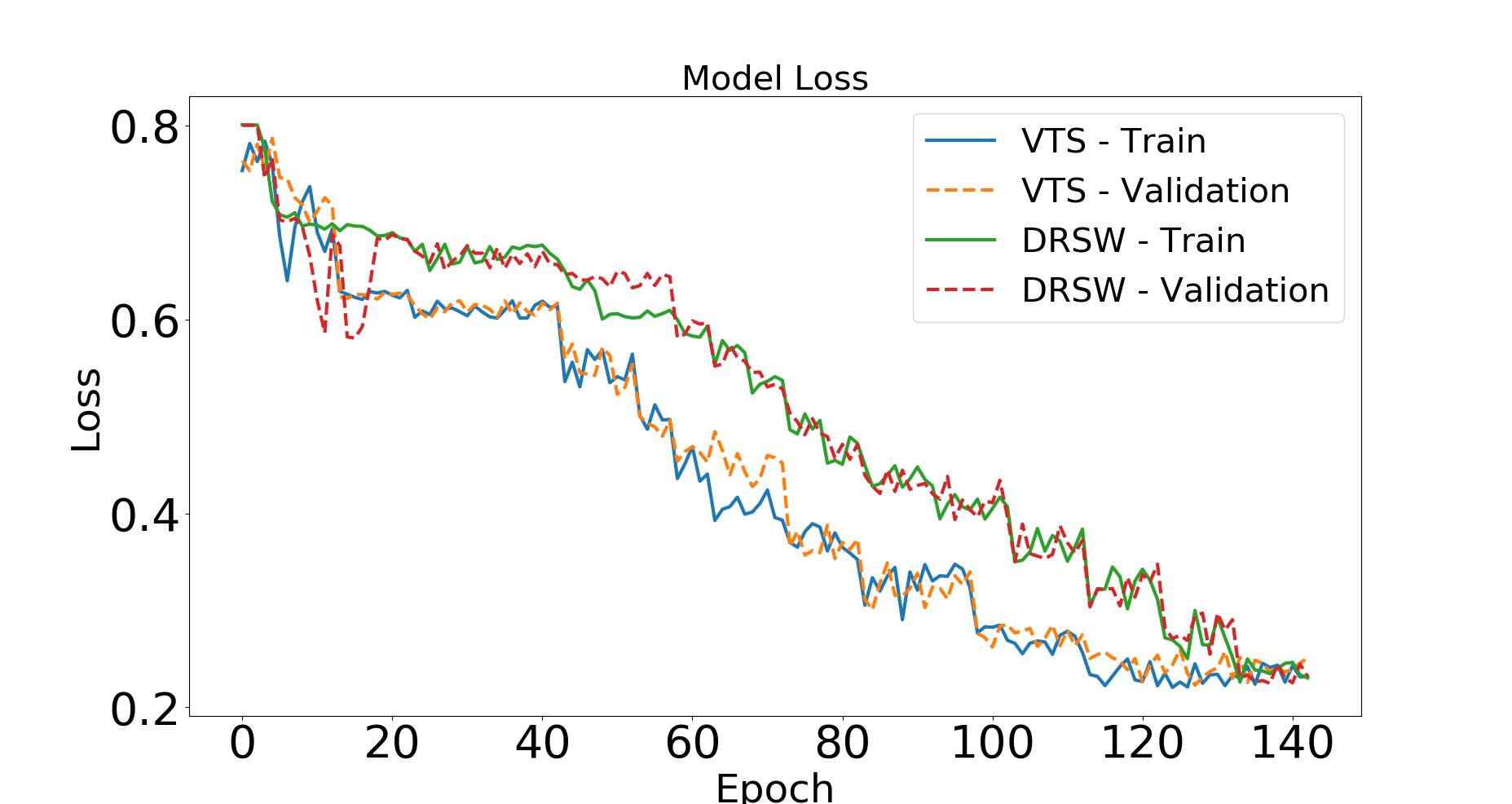
Figure 2: Comparisons between the Two Routing Algorithms

To better understand the importance of different components of our approach, we evaluate the effect of various aspects of the TreeCaps models. This subsection provides a robustness analysis and a comparison between DRSW algorithm and VTS algorithm.

Robustness of Models

We measure the robustness of each model by applying the semantically-preserving program transformations to the Java-large’s test set for the function name prediction task. We follow Wang and Su (2019); Rabin et al. (2020) to transform programs in three ways that change code syntax but preserve code functionality: (1) Variable Renaming (VN), a refactoring transformation that renames a variable in code, where the new name of the variable is taken randomly from a set of variable vocabulary in the training set; (2) Unused Statement (US), inserting an unused string declaration to a randomly selected basic block in the code; and (3) Permute Statement (PS), swapping two independent statements (i.e., with no dependence) in a basic block in the code.

The Java-large test set is thus transformed into a new test set. We then examine if the models make the same predictions for the programs after transformation as the prior predictions for the original programs. We use percentage of predictions changed ($PPC$) as the metric used by (Rabin et al. 2020; Zhang et al. 2020; Wang and Su 2019) to measure the robustness of the code models. Formally, suppose $P$ denotes a set of test programs, a semantic-preserving program transformation $T$ that transforms $P$ into a set of transformed programs $P^{\prime}=\{p^{\prime}=T(p)|p\in P\}$, and a source code model $M$ that can make predictions for any program $p$: $M(p)=l$, where $l\in L$ denotes a predicted label for $p$ according to a set of labels $L$ learned by $M$, we compute the percentage of predictions changed as:

$$PPC=\frac{|\{p^{\prime}\in P^{\prime}|M(p)\neq M(p^{\prime})\}}{|\{p^{\prime}\in P^{\prime}\}|}*100$$ (4)

Lower $PPC$ values for $M$ suggest higher robustness as they can maintain more of correct predictions with respect to the transformation. As shown in Table 3, TreeCaps-VTS is the most robust model against the program transformations. Although more kinds of program transformations could be applied to evaluate model robustness in our future work, the current analysis gives us the confidence that TreeCaps can be more robust against attacks via adversarial examples (Ramakrishnan et al. 2020; Bielik and Vechev 2020).

Comparison between the Two Routing Algorithms

Figure 2 shows the comparisons between the Dynamic Routing algorithm with Shared Weights (DRSW) and Variable-to-Static Routing algorithm (VTS) for the code classification task on the OJ Dataset. There are two main observations: (1) when DRSW is used, the loss decreases slower than when VTS is used (in the right plot); and (2) VTS improves validation accuracy faster than DRSW (in the left chart). A reason is that DRSW has to learn an additional shared transformation matrix $\mathbf{W_{s}}$, resulting in slower convergence due to a larger number of parameters to be learned.

Discussion

Choice of Node Feature Extractor

For the step to extract the node features, we chose TBCNN because it was designed to process ASTs that usually contain deeper and larger numbers of nodes per code snippet than natural language parse trees per sentence, and it has been shown to outperform TreeLSTM in software engineering tasks such as code classification (Mou et al. 2016) and NLP tasks such as natural language inference (Mou et al. 2015).

Relationship with Global Model of Source Code

GREAT (Hellendoorn et al. 2019) is a hybrid approach to combine sequence-based and graph-based model to better capture both local and global features of code. TreeCaps shares the same synergy but with a different approach. The feature extraction step is to extract local features of the source code and the routing mechanism of the capsules is to combine the global features of the source code. We have shown in our evaluation that our capsule-based method performs better than GREAT, both in terms of F1 score and training time. Further research is needed to explore how different types of features are captured inside the capsules.

Conclusion

We propose TreeCaps, a novel neural network architecture that incorporates tree-based convolutional neural networks (TBCNN) into capsule networks for better learning of code on abstract syntax trees. To handle dynamic numbers of capsules produced from TBCNN, we propose two methods to route the capsules in the Primary Variable Capsule layer to a fixed number of capsules in the Secondary Capsule layer. We are the first to re-purpose capsule networks over syntax trees to learn code without the need for explicit semantics analysis. Our empirical evaluations have shown that TreeCaps can outperform existing code learning models (e.g., Code2vec, TBCNN, ASTNN, GGNN, GREAT, GNN-FiLM) for two different program comprehension tasks (e.g., code functionality classification and function name prediction) on C/C++/Java programs. It is our belief that the new method can be applied to other software engineering tasks such as bug localization and clone detection.

A limitation of TreeCaps is similar to the original capsule networks and many other neural networks: it still lacks explainability. Software developers may require additional evidence before accepting the predication results, which suggests future work that relating TreeCaps outputs to certain visible patterns in code could help explain the predictions.

References

- Allamanis, Brockschmidt, and Khademi (2018) Allamanis, M.; Brockschmidt, M.; and Khademi, M. 2018. Learning to Represent Programs with Graphs. In International Conference on Learning Representations.
- Alon et al. (2019a) Alon, U.; Brody, S.; Levy, O.; and Yahav, E. 2019a. code2seq: Generating Sequences from Structured Representations of Code. In International Conference on Learning Representations. URL https://openreview.net/forum?id=H1gKYo09tX.
- Alon et al. (2019b) Alon, U.; Zilberstein, M.; Levy, O.; and Yahav, E. 2019b. Code2Vec: Learning Distributed Representations of Code. Proc. ACM Programming Languages 3(POPL): 40:1–40:29.
- Ben-Nun, Jakobovits, and Hoefler (2018) Ben-Nun, T.; Jakobovits, A. S.; and Hoefler, T. 2018. Neural code comprehension: A learnable representation of code semantics. In Advances in Neural Information Processing Systems, 3585–3597.
- Bielik and Vechev (2020) Bielik, P.; and Vechev, M. 2020. Adversarial Robustness for Code. arXiv preprint arXiv:2002.04694 .
- Britton et al. (2012) Britton, T.; Jeng, L.; Carver, G.; and Cheak, P. 2012. Quantify the time and cost saved using reversible debuggers. Technical report, Cambridge Judge Business School.
- Brockschmidt (2019) Brockschmidt, M. 2019. Gnn-film: Graph neural networks with feature-wise linear modulation. arXiv preprint arXiv:1906.12192 .
- Brockschmidt et al. (2019) Brockschmidt, M.; Allamanis, M.; Gaunt, A. L.; and Polozov, O. 2019. Generative Code Modeling with Graphs. In 7th International Conference on Learning Representations, ICLR 2019, New Orleans, LA, USA, May 6-9, 2019. OpenReview.net. URL https://openreview.net/forum?id=Bke4KsA5FX.
- Bui, Jiang, and Yu (2018) Bui, N. D. Q.; Jiang, L.; and Yu, Y. 2018. Cross-Language Learning for Program Classification Using Bilateral Tree-Based Convolutional Neural Networks. In The Workshops of the The Thirty-Second AAAI Conference on Artificial Intelligence, New Orleans, Louisiana, USA, February 2-7, 2018, volume WS-18 of AAAI Workshops, 758–761. AAAI Press. URL https://aaai.org/ocs/index.php/WS/AAAIW18/paper/view/17338.
- Bui, Yu, and Jiang (2019) Bui, N. D. Q.; Yu, Y.; and Jiang, L. 2019. SAR: learning cross-language API mappings with little knowledge. In Dumas, M.; Pfahl, D.; Apel, S.; and Russo, A., eds., Proceedings of the ACM Joint Meeting on European Software Engineering Conference and Symposium on the Foundations of Software Engineering, ESEC/SIGSOFT FSE 2019, Tallinn, Estonia, August 26-30, 2019, 796–806. ACM. doi:10.1145/3338906.3338924. URL https://doi.org/10.1145/3338906.3338924.
- Chen, Liu, and Song (2018) Chen, X.; Liu, C.; and Song, D. 2018. Tree-to-tree neural networks for program translation. In Advances in Neural Information Processing Systems, 2547–2557.
- Collard, Decker, and Maletic (2013) Collard, M. L.; Decker, M. J.; and Maletic, J. I. 2013. srcML: An Infrastructure for the Exploration, Analysis, and Manipulation of Source Code: A Tool Demonstration. In 2013 IEEE International Conference on Software Maintenance, Eindhoven, The Netherlands, September 22-28, 2013, 516–519. IEEE Computer Society. doi:10.1109/ICSM.2013.85. URL https://doi.org/10.1109/ICSM.2013.85.
- Dahl et al. (2013) Dahl, G. E.; Stokes, J. W.; Deng, L.; and Yu, D. 2013. Large-scale malware classification using random projections and neural networks. In IEEE International Conference on Acoustics, Speech and Signal Processing, 3422–3426. IEEE.
- Evans Data Corporation (2019) Evans Data Corporation. 2019. Global Developer Population and Demographic Study. http://evansdata.com/reports/viewRelease.php?reportID=9.
- Fernandes, Allamanis, and Brockschmidt (2019) Fernandes, P.; Allamanis, M.; and Brockschmidt, M. 2019. Structured Neural Summarization. In 7th International Conference on Learning Representations, ICLR 2019, New Orleans, LA, USA, May 6-9, 2019. OpenReview.net. URL https://openreview.net/forum?id=H1ersoRqtm.
- Gu et al. (2017) Gu, X.; Zhang, H.; Zhang, D.; and Kim, S. 2017. DeepAM: Migrate APIs with Multi-modal Sequence to Sequence Learning. In International Joint Conference on Artificial Intelligence, 3675–3681.
- Gupta, Kanade, and Shevade (2019) Gupta, R.; Kanade, A.; and Shevade, S. 2019. Neural Attribution for Semantic Bug-Localization in Student Programs. In Advances in Neural Information Processing Systems, 11861–11871.
- Hellendoorn et al. (2019) Hellendoorn, V. J.; Sutton, C.; Singh, R.; Maniatis, P.; and Bieber, D. 2019. Global relational models of source code. In International Conference on Learning Representations.
- Hinton, Sabour, and Frosst (2018) Hinton, G. E.; Sabour, S.; and Frosst, N. 2018. Matrix capsules with EM routing. In International Conference on Learning Representations.
- Hu et al. (2018) Hu, X.; Li, G.; Xia, X.; Lo, D.; and Jin, Z. 2018. Deep code comment generation. In International Conference on Program Comprehension, 200–210. ACM.
- Jayasundara et al. (2019) Jayasundara, V.; Jayasekara, S.; Jayasekara, H.; Rajasegaran, J.; Seneviratne, S.; and Rodrigo, R. 2019. TextCaps: Handwritten Character Recognition With Very Small Datasets. In IEEE Winter Conference on Applications of Computer Vision, 254–262.
- Li et al. (2019) Li, C.; Quan, C.; Peng, L.; Qi, Y.; Deng, Y.; and Wu, L. 2019. A capsule network for recommendation and explaining what you like and dislike. In Proceedings of the 42nd International ACM SIGIR Conference on Research and Development in Information Retrieval, 275–284.
- Li et al. (2017) Li, J.; He, P.; Zhu, J.; and Lyu, M. R. 2017. Software defect prediction via convolutional neural network. In IEEE International Conference on Software Quality, Reliability and Security, 318–328. IEEE.
- Li et al. (2016) Li, Y.; Tarlow, D.; Brockschmidt, M.; and Zemel, R. 2016. Gated Graph Sequence Neural Networks. In International Conference on Learning Representations.
- Li et al. (2018) Li, Z.; Zou, D.; Xu, S.; Ou, X.; Jin, H.; Wang, S.; Deng, Z.; and Zhong, Y. 2018. VulDeePecker: A deep learning-based system for vulnerability detection. arXiv preprint arXiv:1801.01681 .
- Liu et al. (2019) Liu, L.; Jiang, H.; He, P.; Chen, W.; Liu, X.; Gao, J.; and Han, J. 2019. On the variance of the adaptive learning rate and beyond. arXiv preprint arXiv:1908.03265 .
- Mou et al. (2016) Mou, L.; Li, G.; Zhang, L.; Wang, T.; and Jin, Z. 2016. Convolutional neural networks over tree structures for programming language processing. In AAAI Conference on Artificial Intelligence.
- Mou et al. (2015) Mou, L.; Peng, H.; Li, G.; Xu, Y.; Zhang, L.; and Jin, Z. 2015. Discriminative Neural Sentence Modeling by Tree-Based Convolution. In Màrquez, L.; Callison-Burch, C.; Su, J.; Pighin, D.; and Marton, Y., eds., Proceedings of the 2015 Conference on Empirical Methods in Natural Language Processing, EMNLP 2015, Lisbon, Portugal, September 17-21, 2015, 2315–2325. The Association for Computational Linguistics. doi:10.18653/v1/d15-1279. URL https://doi.org/10.18653/v1/d15-1279.
- Nghi, Yu, and Jiang (2019) Nghi, B. D. Q.; Yu, Y.; and Jiang, L. 2019. Bilateral Dependency Neural Networks for Cross-Language Algorithm Classification. In Wang, X.; Lo, D.; and Shihab, E., eds., 26th IEEE International Conference on Software Analysis, Evolution and Reengineering, SANER 2019, Hangzhou, China, February 24-27, 2019, 422–433. IEEE. doi:10.1109/SANER.2019.8667995. URL https://doi.org/10.1109/SANER.2019.8667995.
- Nielson, Nielson, and Hankin (1999) Nielson, F.; Nielson, H. R.; and Hankin, C. 1999. Principles of Program Analysis. Berlin, Heidelberg: Springer-Verlag. ISBN 3540654100.
- Nix and Zhang (2017) Nix, R.; and Zhang, J. 2017. Classification of Android apps and malware using deep neural networks. In International Joint Conference on Neural Networks, 1871–1878.
- Pascanu et al. (2015) Pascanu, R.; Stokes, J. W.; Sanossian, H.; Marinescu, M.; and Thomas, A. 2015. Malware classification with recurrent networks. In IEEE International Conference on Acoustics, Speech and Signal Processing, 1916–1920. IEEE.
- Pradel and Sen (2018) Pradel, M.; and Sen, K. 2018. DeepBugs: A learning approach to name-based bug detection. Proceedings of the ACM on Programming Languages 2(OOPSLA): 147.
- Rabin et al. (2020) Rabin, M.; Islam, R.; Bui, N. D.; Yu, Y.; Jiang, L.; and Alipour, M. A. 2020. On the Generalizability of Neural Program Analyzers with respect to Semantic-Preserving Program Transformations. arXiv preprint arXiv:2008.01566 .
- Rajasegaran et al. (2019) Rajasegaran, J.; Jayasundara, V.; Jayasekara, S.; Jayasekara, H.; Seneviratne, S.; and Rodrigo, R. 2019. DeepCaps: Going Deeper with Capsule Networks. In Computer Vision and Pattern Recognition.
- Ramakrishnan et al. (2020) Ramakrishnan, G.; Henkel, J.; Wang, Z.; Albarghouthi, A.; Jha, S.; and Reps, T. 2020. Semantic Robustness of Models of Source Code. arXiv preprint arXiv:2002.03043 .
- Rastogi, Chen, and Jiang (2013) Rastogi, V.; Chen, Y.; and Jiang, X. 2013. Catch me if you can: Evaluating android anti-malware against transformation attacks. IEEE Transactions on Information Forensics and Security 9(1): 99–108.
- Sabour, Frosst, and Hinton (2017) Sabour, S.; Frosst, N.; and Hinton, G. E. 2017. Dynamic routing between capsules. In Conference on Neural Information Processing Systems, 3856–3866. Long Beach, CA.
- Wang and Su (2019) Wang, K.; and Su, Z. 2019. Learning blended, precise semantic program embeddings. ArXiv, vol. abs/1907.02136 .
- Xia et al. (2018) Xia, X.; Bao, L.; Lo, D.; Xing, Z.; Hassan, A. E.; and Li, S. 2018. Measuring Program Comprehension: A Large-Scale Field Study with Professionals. IEEE Transactions on Software Engineering 44(10): 951–976.
- Yang et al. (2018) Yang, M.; Zhao, W.; Ye, J.; Lei, Z.; Zhao, Z.; and Zhang, S. 2018. Investigating Capsule Networks with Dynamic Routing for Text Classification. In Riloff, E.; Chiang, D.; Hockenmaier, J.; and Tsujii, J., eds., Proceedings of the 2018 Conference on Empirical Methods in Natural Language Processing, Brussels, Belgium, October 31 - November 4, 2018, 3110–3119. Association for Computational Linguistics. doi:10.18653/v1/d18-1350. URL https://doi.org/10.18653/v1/d18-1350.
- Yang et al. (2015) Yang, X.; Lo, D.; Xia, X.; Zhang, Y.; and Sun, J. 2015. Deep Learning for Just-in-Time Defect Prediction. In IEEE International Conference on Software Quality, Reliability and Security, 17–26.
- Yu (2019) Yu, Y. 2019. fAST: flattening abstract syntax trees for efficiency. In Atlee, J. M.; Bultan, T.; and Whittle, J., eds., Proceedings of the 41st International Conference on Software Engineering: Companion Proceedings, ICSE 2019, Montreal, QC, Canada, May 25-31, 2019, 278–279. IEEE / ACM. doi:10.1109/ICSE-Companion.2019.00113. URL https://doi.org/10.1109/ICSE-Companion.2019.00113.
- Zhang et al. (2020) Zhang, H.; Li, Z.; Li, G.; Ma, L.; Liu, Y.; and Jin, Z. 2020. Generating Adversarial Examples for Holding Robustness of Source Code Processing Models. In 34th AAAI Conference on Artificial Intelligence.
- Zhang et al. (2019) Zhang, J.; Wang, X.; Zhang, H.; Sun, H.; Wang, K.; and Liu, X. 2019. A novel neural source code representation based on abstract syntax tree. In International Conference on Software Engineering, 783–794.
- Zhang and Chen (2019) Zhang, X.; and Chen, L. 2019. Capsule Graph Neural Network. In International Conference on Learning Representations.
- Zhou et al. (2019) Zhou, Y.; Liu, S.; Siow, J. K.; Du, X.; and Liu, Y. 2019. Devign: Effective Vulnerability Identification by Learning Comprehensive Program Semantics via Graph Neural Networks. In Wallach, H. M.; Larochelle, H.; Beygelzimer, A.; d’Alché-Buc, F.; Fox, E. B.; and Garnett, R., eds., Advances in Neural Information Processing Systems 32: Annual Conference on Neural Information Processing Systems 2019, NeurIPS 2019, 8-14 December 2019, Vancouver, BC, Canada, 10197–10207. URL http://papers.nips.cc/paper/9209-devign-effective-vulnerability-identification-by-learning-comprehensive-program-semantics-via-graph-neural-networks.