Improving Robustness and Generality of NLP Models
Using Disentangled Representations

Abstract

Supervised neural networks, which first map an input $x$ to a single representation $z$, and then map $z$ to the output label $y$, have achieved remarkable success in a wide range of natural language processing (NLP) tasks. Despite their success, neural models lack for both robustness and generality: small perturbations to inputs can result in absolutely different outputs; the performance of a model trained on one domain drops drastically when tested on another domain.

In this paper, we present methods to improve robustness and generality of NLP models from the standpoint of disentangled representation learning. Instead of mapping $x$ to a single representation $z$, the proposed strategy maps $x$ to a set of representations $\{z_{1},z_{2},...,z_{K}\}$ while forcing them to be disentangled. These representations are then mapped to different logits $l$s, the ensemble of which is used to make the final prediction $y$. We propose different methods to incorporate this idea into currently widely-used models, including adding an $L$2 regularizer on $z$s or adding Total Correlation (TC) under the framework of variational information bottleneck (VIB). We show that models trained with the proposed criteria provide better robustness and domain adaptation ability in a wide range of supervised learning tasks.

1 Introduction

Supervised neural networks have achieved remarkable success in a wide range of NLP tasks, such as language modeling (Xie et al., 2017; Devlin et al., 2018a; Liu et al., 2019; Joshi et al., 2020; Meng et al., 2019b), machine reading comprehension (Seo et al., 2016; Yu et al., 2018), and machine translation (Sutskever et al., 2014; Vaswani et al., 2017b; Meng et al., 2019a). Despite the success, neural models lack for both robustness and generality and are extremely fragile: the output label can be changed with a minor change of a single pixel Szegedy et al. (2013); Goodfellow et al. (2014b); Nguyen et al. (2015); Papernot et al. (2017); Yuan et al. (2019) in an image or a token in a document Li et al. (2016); Papernot et al. (2016); Jia and Liang (2017); Zhao et al. (2017); Ebrahimi et al. (2017); Jia et al. (2019b); The model lacks for domain adaptation abilities Mou et al. (2016); Daumé III (2009): a model trained on one domain can hardly generalize to new test distributions Fisch et al. (2019); Levy et al. (2017). Despite that different avenues have been proposed to address model robustness such as augmenting the training data using rule-based lexical substitutions Liang et al. (2017); Ribeiro et al. (2018) or paraphrase models Iyyer et al. (2018), building robust and domain-adaptive neural models remains a challenge.

In a standard supervised learning setup, a neural network model first maps an input $x$ to a single vector $z=f(x)$. $z$ can be viewed as the hidden feature to represent $x$, and is transformed to its logit $l$ followed by a softmax operator to output the target label $y$. At training time, parameters involved in mapping from $x\in X$ to $z$ then to $y$ are learned. At test time, the pretrained model makes a prediction when presented with a new instance $x^{\prime}\in X^{\prime}$. This methodology works well if $X$ and $X^{\prime}$ come from exactly the same distribution, but significantly suffers if not. This is because the implicit representation learned through supervised signals can easily and overfit to the training domain $X$, and the mapping function $f(x)$, which is trained only based on $X$, can be confused with out-of-domain features in $x^{\prime}$, such as a lexical, pragmatic, and syntactic variation not seen in the training set Ettinger et al. (2017). We can also interpret the weakness of this methodology from a domain adaptation point of view Daume III and Marcu (2006); Daumé III (2009); Tan et al. (2009); Patel et al. (2014): it is crucial to separate source-specific features, target-specific features and general features (features shared by sources and targets). One of the most naive strategies for domain adaptation is to ask the model to only use general features for test. In the standard $x\rightarrow z\rightarrow y$ setup, all features, including source-specific, target-specific and general features, are entangled in $z$. Due to the lack of interpretability Li et al. (2015); Linzen et al. (2016); Lei et al. (2016); Koh and Liang (2017) of neural models, it is impossible to disentangle them.

Inspired by recent work in disentangled representation learning Bengio et al. (2013); Kim and Mnih (2018); Hjelm et al. (2018); Kumar et al. (2018); Locatello et al. (2019), we propose to improve robustness and generality of NLP models using disentangled representations. Different from mapping $x$ to a single representation $z$ and then to $y$, the proposed strategy first maps $x$ to a set of distinct representations $Z=\{z_{1},\cdots,z_{K}\}$, which are then individually projected to logits $l_{1},\cdots,l_{K}$. $l$s are ensembled to make the final prediction of $y$. In this setup, we wish to make $z$s or $l$s to be disentangled from each other as much as possible, which potentially improves both robustness and generality: For the former, the decision of $y$ is more immune to small changes in $x$ since even though small changes lead to significant changes in some $z$s or $l$s, others may remain invariant. The ultimate influence on $y$ can be further regulated when $l$s are combined. For the latter, different $l$s have the potential to disentangle or partially disentangle source-specific, target-specific and general features.

Practically, we propose two ways to disentangle representations: adding an $L$2 regularizer or adding Total Correlation (TC) (Cover and Thomas, 2012; Ver Steeg and Galstyan, 2015; Steeg, 2017; Gao et al., 2018; Chen et al., 2018) under the framework of variational information bottleneck (VIB). We show that models trained with the proposed criteria provide better robustness and domain adaptation ability in a wide range of NLP tasks, with tiny or non-significant sacrifice on task-specific accuracies.

In summary, the contributions of this paper are:

• We present two methods to improve the robustness and generality of NLP models in the view of disentangled representation learning and the information bottleneck theory.

• Extensive experiments on domain adaptation and defense against adversarial attacks show that the proposed methods are able to provide better robustness compared with conventional task-specific models, which indicates the effectiveness of the theory of information bottleneck and disentangled representation learning for NLP tasks.

The rest of this paper is organized as follows: we present related work in Section 2. Models are detailed in Section 3 and Section 4. We present experimental results and analysis in Section 5, followed by a brief conclusion in Section 6.

2 Related Work

2.1 Learning Disentangled Representations

Disentangled representation learning was first proposed by Bengio et al. (2013). InfoGan (Chen et al., 2016) disentangled the representation by maximizing the mutual information between a small subset of the GAN’s noise latent variables and the observation. Kim and Mnih (2018) learned disentangled representations in VAE, by encouraging the distribution of representations to be factorial and hence independent across the dimensions. Hjelm et al. (2018) learned disentangled representations by simultaneously estimating and maximizing the mutual information between input data and learned high-level representations. Chen et al. (2018) proposed $\beta$-TCVAE, encouraging the model to find statistically independent factors in the data distribution by imposing a total correlation (TC) penalty. Similarly, Kumar et al. (2018) learned disentangled latents from unlabeled observations by introducing a regularizer over the induced prior.

2.2 The Information Bottleneck Principle

The Information Bottleneck (IB) principle was first proposed by Tishby et al. (2000). It treats the supervised learning task as an optimization problem that squeezes the information from an input about the output through an information bottleneck. In information bottleneck, the mutual information $I(X;Y)$ is used as the measurement of the relevant information between $x$ and the output $y$. Tishby and Zaslavsky (2015); Shwartz-Ziv and Tishby (2017) proposed to use it as a theoretical tool for analyzing and understanding representations in deep neural networks. Alemi et al. (2016) proposed a deep variational version of the IB principle (VIB) to allow for using deep neural networks to parameterize the distributions. In the field of NLP, not much attention has been attached to the Information Bottleneck principle. Li and Eisner (2019) proposed to extract specific information for different tasks (which are defined in the output $y$) from pretrained word embeddings using VIB. Less relevant work is from Kong et al. (2019), which proposed a self-supervised objective that maximizes the mutual information between global sentence representations and $n$-grams in the sentence.

2.3 Domain Adaptation in NLP

Domain adaptation evalutes the model’s ability of generalization across domains, for which many efforts have been devoted to designing more powerful cross-domain models (Daumé III, 2009; Kim et al., 2015; Lee et al., 2018; Adel et al., 2017; Yang et al., 2018; Ruder, 2019). Sun et al. (2016) proposed CORAL, a method that minimizes domain shift by aligning the second-order statistics of source and target distributions without even requiring any target labels; Lin and Lu (2018) added domain-adaptive layers on top of the model; Jia et al. (2019a) used cross-domain language models as a bridge cross-domains for domain adaptation. Li et al. (2019b); Du et al. (2020) applied adversarial learning to learn cross-domain models for the task of sentiment analysis. For machine translation, the core idea is to utilize large available parallel data for training NMT models and adapt them to domains with small data (Chu et al., 2017), where data augmentation (Sennrich et al., 2016a; Ul Haq et al., 2020), meta-learning (Gu et al., 2018) and finetuning methods (Luong and Manning, 2015; Freitag and Al-Onaizan, 2016; Dakwale, 2017) are proposed to achieve this goal.

2.4 Defense against Adversarial Attacks in NLP

Deep neural networks are fragile when attacked by adversarial examples (Goodfellow et al., 2014a; Arjovsky et al., 2017; Mirza and Osindero, 2014). In the context of NLP, Sato et al. (2018) built a candidate pool that includes adversarial examples, and used the method of Fast Gradient Sign Method (FGSM) (Goodfellow et al., 2014b) to select a candidate word for replacement. Papernot et al. (2016b) showed that the forward derivative (Papernot et al., 2016a) can be used to produce adversarial sequences manipulating both the sequence output and classification predictions made by an RNN. Liang et al. (2017) designed three perturbation strategies for word-level attack — insertion, modification and removal. Miyato et al. (2016); Sato et al. (2018); Zhu et al. (2020); Zhou et al. (2020) restricted the directions of perturbations toward the existing words in the input embedding space. Ebrahimi et al. (2017) proposed a novel token transformation method by computing derivatives with respect to a few character-edit operations. Other methods either generate certified defenses (Jia et al., 2019b; Huang et al., 2019; Shi et al., 2020), or generate examples that maintain lexical correctness, grammatical correctness and semantic similarity (Ren et al., 2019a).

3 Adding $L_{2}$ Regularizer on $Z$

Here, we present our first attempt to learn disentangled representations with an $L_{2}$ regularizer. We first map the input $x$ to multiple representations $Z=\{z_{1},z_{2},...,z_{K}\}$ and we wish different $z$s to be disentangled. To obtain $Z$, we can use independent sets of parameters of RNNs Hochreiter and Schmidhuber (1997); Mikolov et al. (2010), CNNs Krizhevsky et al. (2012); Kalchbrenner et al. (2014) or Transformers Vaswani et al. (2017b). This actually mimics the idea of the model ensemble. To avoid the parameter and memory intensity in the ensemble setup, we adopt the following simple method: we first map $x$ to a single vector representation $z$ using RNNs or CNNs. Next, we separate sub-representations from $z$ using distinct projection matrices, each of which tries to capture a certain aspect of features, given as follows:

$$z_{i}=W_{i}z,\;i=1,\cdots,K$$ (1)

where $z$, $z_{i}\in\mathbb{R}^{d\times 1}$, $W_{i}\in\mathbb{R}^{d\times d}$, and $K$ is the number of disentangled representations.

To make sure that these sub-representations actually disentangle, we enforce a regularizer on the $L_{2}$ distance between each pair of them:

$$\mathcal{L}_{\text{reg}}=\sum_{ij}\|z_{i}-z_{j}\|^{2}$$ (2)

The regularizer assumes that the distance between representations in the Euclidean space is in accordance with the distinctiveness between features that are the most salient for predictions. Each $z_{i}$ is next mapped to a logit $l_{i}$ as follows:

$$l_{i}=W\cdot z_{i},\;i=1,\cdots,K$$ (3)

where $W\in\mathbb{R}^{T\times d}$ and $T$ denotes the number of predefined classes for the supervised learning task. Next we aggregate the weighted logits into a single final logit $l=\sum\alpha_{i}l_{i}$, where $\alpha_{i}$ is the weight associated with $l_{i}$. $\alpha_{i}$ can be computed using the softmax operator by introducing a learnable parameter $w_{a}\in\mathbb{R}^{d\times 1}$:

$$\bm{\alpha}=\texttt{softmax}([z_{1}^{\top}w_{a},\cdots,z_{K}^{\top}w_{a}])$$ (4)

Combining the cross entropy loss with golden label $\hat{y}$ and the $L_{2}$ regularizer on $Z$, we can obtain the final training objective as follow:

$$\mathcal{L}_{\text{separare}}=\text{CE}(\texttt{softmax}(l),\hat{y})+\beta\mathcal{L}_{\text{reg}}$$ (5)

$\beta$ is the hyper-parameter controlling the weight of the regularizer. The method can be adapted to any neural network. Albeit simple, this model has significantly better ability of learning disentangled features and and is less prone to adversarial attacks, as we will show in the experiments later.

4 Variational Information Bottleneck with Total Correlation

Many recent works (Alemi et al., 2016; Higgins et al., 2017; Burgess et al., 2018) have shown that the information bottleneck is more suitable for learning robust and general features than task-specific end-to-end models, due to the flexibility provided by its learned structure. Here we first go through the preliminaries of the variational information bottleneck (VIB) Alemi et al. (2016), and then detail how it can be adapted for learning disentangled representations by adding a Total Correlation (TC) regularizer (Ver Steeg and Galstyan, 2015; Steeg, 2017; Gao et al., 2018).

4.1 Variational Information Bottleneck

Let $p(z|x)$ denote an encoding of $x$, which maps $x$ to representations $z$. The key point of IB is to learn an encoding that is maximally informative about our target $Y$, measured by the mutual information between $z$ and the target $y$, denoted by $I(y,z)$. Unfortunately, only modeling $I(y,z)$ is not enough since the model can always make $z=x$ to ensure the maximally informative representation, which is not helpful for learning general features. Instead, we need to find the best $z$ subject to a constraint on its complexity, leading to the penalty on the mutual information between $x$ and $z$. The objective for IB is thus given as follows:

$$\mathcal{L}_{\text{IB}}=I(z,y;\bm{\theta})-\beta I(z,x;\bm{\theta})$$ (6)

where $\beta$ controls the trade-off between $I(z,y)$ and $I(z,x)$. Intuitively, the first term encourages $z$ to be predictive of $y$ and the second term enforces $z$ to be concisely representative of $x$.

By leaving details to the appendix, we can obtain the lower bound of $I(z,y)$ and the upper bound of $I(z,x)$:

$$I(z,y)\geq\int p(x)p(y|x)p(z|x)\log q(y|z)\ \mathrm{d}x\mathrm{d}y\mathrm{d}z$$ (7)

$$I(z,x)\leq\int p(x)p(z|x)\log\frac{p(z|x)}{r(z)}\ \mathrm{d}x\mathrm{d}z$$

where $q(y|z)$ and $r(z)$ are variational approximations to $p(y|z)$ and $p(z)$ respectively. We can immediately have the lower bound of Eq.6:

$$I(Z,Y)-\beta I(Z,X)\geq$$ (8)

$$\int p(x)p(y|x)p(z|x)\log q(y|z)\ \mathrm{d}x\mathrm{d}y\mathrm{d}z$$

$$-\beta\int p(x)p(z|x)\log\frac{p(z|x)}{r(z)}\ \mathrm{d}x\mathrm{d}z=\mathcal{L}_{\text{VIB}}$$

In order to compute this in practice, we approximate $p(x,y)$ using the empirical data distribution $p(x,y)=\frac{1}{N}\sum_{n=1}^{N}\delta_{x_{n}}(x)\delta_{y_{n}}(y)$, leading to:

$$\mathcal{L}_{\text{VIB}} \approx\frac{1}{N}\sum_{n=1}^{N}\left[\int p(z|x_{n})\log q(y_{n}|z)\ \mathrm{d}z-\right.$$ (9)

$$\left.\beta p(z|x_{n})\log\frac{p(z|x_{n})}{r(z)}\right]$$

By using the reparameterization trick (Kingma and Welling, 2013) to rewrite $p(z|x)\mathrm{d}z=p(\epsilon)\ \mathrm{d}\epsilon$, where $z=f(x,\epsilon)$ is a deterministic function of $x$ and the Guassian random variable $\epsilon$, we put everything together to the following objective:

$$\mathcal{L}_{\text{VIB}}= \frac{1}{N}\sum_{n=1}^{N}\mathbb{E}_{p(\mathbf{\epsilon})}[-\log q(y_{n}|f(x_{n},\mathbf{\epsilon}))]+$$ (10)

$$\beta\mathcal{D}_{\text{KL}}(p(z|x_{n}),r(z))$$

$p(z|x)$ is set to $\mathcal{N}(z|f^{\mu}_{e}(x),f^{\Sigma}_{e}(x))$ where $f_{e}$ is an MLP of mapping the input $x$ to a stochastic encoding $z$. The output dimension of $f_{e}$ is $2D$, where the first $D$ outputs encode $\mu$ and the remaining $D$ outputs encode $\sigma$. Then we sample $\epsilon\sim\mathcal{N}(\mathbf{0},\mathbf{I})$ and combine them together $z=\mu+\epsilon\cdot\sigma$. We treat $r(z)=\mathcal{N}(z|\mathbf{0},\mathbf{I})$ and $q(y|z)$ as a softmax classifier. Eq. 10 can be trained by directly backpropagating through examples and the gradient is an unbiased estimate of the true gradient.

4.2 VIB+TC: VIB with Total Correlation

While VIB provides a neat way of parameterizing the information bottleneck approach and efficiently training the model with the reparameterization trick, the learned representations only contain the minimal statistics required to predict the target label, it does not immediately have the ability to disentangle the learned representations. To tackle this issue, another regularizer is added, the Total Correlation (TC) (Ver Steeg and Galstyan, 2015; Steeg, 2017; Gao et al., 2018), to disentangle $z$:

$$\text{TC}(z_{1},..,z_{K}|x)=\sum_{i=1}^{K}H(z_{i}|x)-H(z_{1},\cdots,z_{K}|x)$$ (11)

$$=\mathcal{D}_{\text{KL}}\left[p(z_{1},\cdots,z_{K}|x),\prod_{i=1}^{K}p(z_{i}|x)\right]$$

The TC term measures the dependence between $p(z_{i}|x)$s. The penalty on TC forces the model to find statistically independent factors in the features. In particular, $\text{TC}(z_{1},..,z_{K}|x)$ is zero if and only if all $p(z_{i}|x)$s are independent, in which case we say that they are disentangled. Thus, the training objective is defined as follows:

$$\mathcal{L}_{\text{VIB+TC}}=\frac{1}{N}\sum_{i=1}^{K}\sum_{n=1}^{N}\mathbb{E}_{p(\epsilon)}[{-\log q(y_{n}|z_{i})}$$ (12)

$${+\beta\mathcal{D}_{\text{KL}}(p(z_{i}|x_{n}),r(z_{i}))}]$$

$$+\lambda\mathcal{D}_{\text{KL}}\left[p(z_{1},...,z_{K}|x),\prod_{i=1}^{K}p(z_{i}|x)\right]$$

where $\beta$ and $\lambda$ are a hyper-parameters to adjust the trade-off between these two factors. $p(z_{i}|x)$ is set to $\mathcal{N}(z|f^{\mu}_{e,i}(x),f^{\Sigma}_{e,i}(x))$, in a similar way to $p(z|x)$ except that $f^{\mu}_{e,i}(x)$ and $f^{\Sigma}_{e,i}$ are scalars. Eq.12 can also be directly trained with an unbiased estimate of the true gradient.

5 Experiments

In this section, we describe experimental results. We conduct experiments in two NLP subfields: domain adaptation and defense against adversarial attacks.

5.1 Domain Adaptation

The goal of domain adaptation tasks is to test whether a model trained in one domain (source-domain) can work well when test in another domain (target-domain). In the domain adaptation setup, there should be at least labeled source-domain data for training and labeled target-domain data for test. Setups can be different regarding whether there is also a small amount of labeled target-domain data for training or unlabeled target-domain data for unsupervised training Jia et al. (2019a). In this paper, we adopt the most naive setting where there is neither labeled nor unlabeled target-domain data for training to straightforwardly test a model’s ability for domain adaptation. We perform experiments on the following domain adaptation tasks: named entity recognition (NER), part-of-speech tagging (POS), machine translation (MT) and text classification (CLS). The $L_{2}$ regularizer, VIB and VIB+TC models are built on top of representations of the last layer for fair comparison.

Method	NER	POS	MT	CLS-sentiment	CLS-deception
Baseline	97.88	90.12	34.61	87.4	87.5
VIB	98.02+0.14	90.85+0.73	34.90+0.29	88.5+1.1	88.6+1.1
VIB+TC	98.33+0.45	91.43+1.31	35.31+0.70	89.8+2.4	89.3+1.8
Regularizer	98.21+0.33	91.30+1.18	35.13+0.52	89.2+1.8	88.7+1.2

Table 1: Results for domain adaptation. The evaluation metric for NER, POS and CLS is accuracy, and that for MT is the BLEU score (Papineni et al., 2002).

NER

For the task of NER, we followed the setup in Daumé III (2009) and used the ACE06 dataset as the source domain and the CoNLL 2003 NER data as the target domain. The training dataset of ACE06 contains 256,145 examples, and the dev and test datasets from CoNLL03 respectively contains 5,258 and 8,806 examples. For evaluation, we followed Daumé III (2009) and report only on label accuracy. We used the MRC-NER model as the baseline Li et al. (2019a), which achieves SOTA performances on a wide range of NER tasks. All models are trained using using Adam (Kingma and Ba, 2014) with $\beta=(0.9,0.98)$, $\epsilon=10^{-6}$, a polynomial learning rate schedule, warmup up for 4K steps and weight decay with $10^{-3}$.

POS

For the task of POS, we followed the setup in Daumé III (2009). The source domain is the WSJ portion of the Penn Treebank, containing 950,028 training examples. The target domain is PubMed, with the dev and test sets respectively containing 1,987 and 14,554 examples. We used the BERT-large model as the backbone. The model is optimized using Adam (Kingma and Ba, 2014).

Machine Translation

We used the WMT 2014 English-German dataset for training, which contains about 4.5 million sentence pairs. We used the Tedtalk dataset Duh (2018) for test. We use the Transformer-base model Vaswani et al. (2017a) as the backbone, where the encoder and decoder respectively have 6 layers. Sentences are encoded using BPE (Sennrich et al., 2016b), which has a shared source target vocabulary of about 37000 tokens. For fair comparison, we used the Adam optimizer (Kingma and Ba, 2014) with $\beta_{1}$ = 0.9, $\beta_{2}$ = 0.98 and $\epsilon$ = $10^{-9}$ for all models. For the base setup, following Vaswani et al. (2017a), the dimensionality of inputs and outputs $d_{\text{model}}$ is set to 512, and the inner-layer has dimensionality $d_{\text{ff}}$ is set to 2,048.

Text Classification

For text classification, we used two datasets. The first dataset we consider is the sentiment analysis on reviews. We used the 450K Yelp reviews for training and $\sim$ 3k Amazon reviews for test Li et al. (2018). The task is transformed to a binary classification task to decide whether a review is of positive or negative sentiment. We also used the deceptive opinion spam detection dataset Li et al. (2014), a binary text classification task to classify whether a review is fake or not. We used the hotel reviews for training, which consists of 800 reviews in total from customers, and used the 400 restaurant reviews for test. For baselines, we used the BERT-large model (Devlin et al., 2018b) as the backbone, where the [cls] is first mapped to a scalar and then output to a sigmoid function. We report accuracy on the test set.

Results

Results for domain adaptation are shown in Table 1. As can be seen, for all tasks, VIB+TC performs best among all four models, followed by the proposed $L2$ regularizer model, next followed by the VIB model without disentanglement. The vanilla VIB model outperforms the baseline supervised model. This is because the VIB model maps an input to multiple representations, and this operation to some degree separates features in a natural way. The $L2$ regularizer method consistently outperforms VIB and underperforms VIB+TC. This is because VIB+TC uses the TC term to disentangle features deliberately, and the vanilla VIB model does not have this property. Experimental results demonstrate the importance of learning disentangled features in domain adaptation.

IMDB
Method	BoW				CNN				LSTM
	Clean	PWWS	GA${}_{\text{w/LM}}$	GA${}_{\text{w/o LM}}$	Clean	PWWS	GA${}_{\text{w/LM}}$	GA${}_{\text{w/o LM}}$	Clean	PWWS	GA${}_{\text{w/LM}}$	GA${}_{\text{w/o LM}}$
Orig.	88.7	12.4	2.1	0.7	90.0	18.1	4.2	2.0	89.7	1.4	2.5	0.1
VIB	88.6	22.4	19.0	11.5	89.3	36.1	34.7	13.1	88.9	14.2	31.4	7.6
VIB+TC	89.1	26.5	21.4	19.5	89.5	40.2	39.0	18.6	89.6	16.9	33.0	10.4
Regularizer	90.1	17.1	7.2	3.7	90.6	21.4	15.1	8.9	90.1	3.1	15.3	5.8
AGNews
Method	BoW				CNN				LSTM
	Clean	PWWS	GA${}_{\text{w/LM}}$	GA${}_{\text{w/o LM}}$	Clean	PWWS	GA${}_{\text{w/LM}}$	GA${}_{\text{w/o LM}}$	Clean	PWWS	GA${}_{\text{w/LM}}$	GA${}_{\text{w/o LM}}$
Orig.	88.4	45.2	58.3	19.5	89.2	37.8	45.7	12.5	92.4	46.8	48.7	9.4
VIB	87.9	57.4	64.5	32.2	88.5	50.4	54.7	21.0	91.4	57.6	59.7	19.2
VIB+TC	87.6	61.4	72.1	34.5	89.0	54.3	59.2	25.4	92.5	61.1	65.4	21.1
Regularizer	88.4	50.1	65.0	25.4	89.4	43.5	50.2	17.5	92.8	50.3	52.1	11.0

Table 2: Results for the IMDB and AGNews datasets. Orig. stands for the original baseline, on which all other methods are based. Accuracy is reported for comparison.

SNLI
Method	Clean	PWWS	GA${}_{\text{w/LM}}$	GA${}_{\text{w/o LM}}$
Orig.	90.5	43.1	55.6	21.4
VIB	89.4	56.5	62.4	35.9
VIB+TC	89.9	62.4	67.0	41.3
Regularizer	90.4	48.1	59.6	27.2

Table 3: Results for the SNLI dataset. We report accuracy for all models.

5.2 Defense Against Adversarial Attacks

We evaluate the proposed methods on tasks for defense against adversarial attacks. We conduct experiments on the tasks of text classification and natural language inference in defense against two recently proposed attacks: PWWS and GA. PWWS Ren et al. (2019b), short for Probability Weighted Word Saliency, performs text adversarial attacks based on word substitutions with synonyms. The word replacement order is determined by both word saliency and prediction probability. GA Alzantot et al. (2018) uses language models to remove candidate substitute words that do not fit within the context. We report the accuracy under GA attacks for both with and without using the LM.

Following Zhou et al. (2020), for text classification, we use two datasets, IMDB (Internet Movie Database) and AG News corpus (Del Corso et al., 2005). IMDB contains 50, 000 movie reviews for binary (positive v.s. negative) sentiment classification, and AGNews contains roughly 30, 000 news articles for 4-class classification. We use three base models: bag-of-words models, CNNs and two-layer LSTMs. The bag-of-words model first averages the embeddings of constituent words of the input, and then passes the average embedding to a feedforward network to get a 100$d$ vector. The vector is then mapped to the final logit. CNNs and LSTMs are used to map input text sequences to vectors, which are fed to sigmoid for IMDB and softmax for AGNews.

For natural language inference, we conduct experiments on the Stanford Natural Language Inference (SNLI) corpus (Bowman et al., 2015). The dataset consists of 570, 000 English sentence pairs. The task is transformed to a 3-class classification problem, giving one of the entailment, contradiction, or neutral label to the sentence pair. All models use BERT as backbones and are trained on the CrossEntropy loss, and their hyper-parameters are tuned on the validation set.

Results

Table 2 shows results for the IMDB and AGNews datasets, and Table 3 shows results for the SNLI dataset. When tested on the clean dataset where no attack is performed, variational methods, i.e., VIB and VIB+TC, underperform the baseline model. This is in line with our expectation: because of the necessity of modeling the KL divergence between $z$ and $x$, the variational methods do not gets to label prediction as straightly as supervised learning models. But variational methods significantly outperform supervised baselines when attacks are performed, which is because of the flexibility offered by the disentangled latent representations. VIB+TC outperforms VIB due to the disentanglement introduced by TC when attacks are present. As expected, the $L2$ regularizer model outperforms the baseline model in terms of robustness in defense against adversarial attacks. It is also interesting that with $L2$ regularizer, the model performs at least comparable to, and sometimes outperforms the baseline in the setup without adversarial attacks, which demonstrates that disentangled representations can also help alleviate overfitting, leading to better performances.

5.3 Ablation Studies

IMDB
$\beta$	Clean	PWWS	GA${}_{\text{w/LM}}$	GA${}_{\text{w/o LM}}$
0	90.0	18.1	4.2	2.0
0.05	90.3	19.7	11.4	6.2
0.10	90.6	21.4	15.1	8.9
0.15	90.1	22.7	17.2	8.8
0.20	89.5	22.3	15.5	7.5
0.25	88.7	20.6	13.2	6.5
0.30	87.9	18.9	11.6	4.5

Table 4: Results of varying the hyperparamter $\beta$ in the Regularizer method. Accuracy is reported for comparison. The backbone model is CNN.

IMDB
$\gamma$	Clean	PWWS	GA${}_{\text{w/LM}}$	GA${}_{\text{w/o LM}}$
0	89.3	36.1	34.7	13.1
0.05	89.5	37.9	37.2	15.1
0.10	89.5	39.1	39.0	17.6
0.15	89.5	40.2	38.8	18.6
0.20	88.4	38.5	38.0	17.9
0.25	87.4	37.2	36.8	16.6
0.30	86.2	36.5	36.5	15.2

Table 5: Results of varying the hyperparamter $\gamma$ in the VIB+TC method. Accuracy is reported for comparison. The backbone model is CNN.

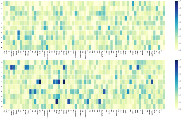
Figure 1: Heatmaps for models without (top) and with (bottom) $L_{2}$ regularizer.

Next, we explore how the strength of the regularization terms in VIB+TC and Regularizer affects performances. Specifically, we vary the coefficient hyperparamter $\beta$ in Regularizer and the $\gamma$ in VIB+TC to show their influences on defending against adversarial attacks. We use the IMDB dataset for evaluation and use CNNs as baselines, and for each setting, we tune all other hyperparamters on the validation set.

Results are shown in Table 4 and Table 5. As can be seen from the tables, when these two hyperparamters are around $0.1\sim 0.15$, the best results are achieved. For both methods, the performance first rises when increasing the hyperparameter value, and then drops as we continue increasing it. Besides, the difference between the best result and the worst result in the same model is surprisingly large (e.g., for the PWWS attack, the difference is 4.6 for Regularizer and 4.1 for VIB+TC), indicating the importance and the sensitivity of the introduced regularizers.

5.4 Visualization

It would be interesting to visualize how the disentangled $z$s encode the information of different parts of the input. Unlike feature-based models like SVMs, it’s intrinsically hard to measure the influence of units of one layer on another layer in an neural architecture (Zeiler and Fergus, 2014; Yosinski et al., 2014; Bau et al., 2017; Koh and Liang, 2017). We turn to the first-derivative saliency method, a widely used tool to visualize the influence of a change in the input on the model’s predictions (Erhan et al., 2009; Simonyan et al., 2013; Li et al., 2015). Specially, we want to visualize the influence of an input token $e$ on the $j$-th dimension of $z_{i}$, denoted by $z_{i}^{j}$. In the case of deep neural models, $z_{i}^{j}$ is a highly non-linear function of $e$. The first-derivative saliency method approximates $z_{i}^{j}$ with a linear function of $e$ by computing the first-order Taylor expansion

$$z_{i}^{j}\approx w_{i}^{j}(e)^{\top}e+b$$ (13)

where $w_{i}^{j}(e)$ is the derivative of $z_{i}^{j}$ with respect to the embedding $e$.

$$w_{i}^{j}(e)=\frac{\partial(z_{i}^{j})}{\partial e}\Big{|}_{e}$$ (14)

The magnitude (absolute value) of the derivative indicates the sensitiveness of the final decision to the change in one particular word embedding, telling us how much one specific token contributes to $z$. By summing over $j$, the influence of $e$ on $z_{i}$ is given as follows:

$$S_{i}(e)=\sum_{j}|w_{i}^{j}(e)|$$ (15)

Figure plots the heatmaps of $S_{i}(e)$ with respect to word input vectors for models with and without the TC regularizer. As can be seen, by pushing representations to be disentangled, different representations are able to encode separate meanings of texts: $z_{1}$ tends to encode more positive information while $z_{4}$ tends to encode negative information. This ability for feature separation and meaning clustering potentially improves the model’s robustness.

6 Conclusion

In this paper, we present methods to improve the robustness and generality on various NLP tasks in the perspective of the information bottleneck theory and disentangled representation learning. In particular, we find the two variational methods VIB and VIB+TC perform well on cross domain and adversarial attacks defense tasks. The proposed simple yet effective end-to-end method of learning disentangled representations with $L_{2}$ regularizer performs comparably well on cross-domain tasks, while better than vanilla non-disentangled models on adversarial attacks defense tasks, which shows the effectiveness of disentangled representations.

Appendix A Derivation of Variational Information Bottleneck

Below we take the derivation of VIB from Alemi et al. (2016).

We first decompose the joint distribution $p(X,Y,Z)$ into:

$$p(X,Y,Z) =p(X)p(Y|X)p(Z|X,Y)$$ (16)

$$=p(X)p(Y|X)p(Z|X)$$

Then, for the first term in the IB objective $I(Z,Y)-\beta I(Z,X)$, we write it out in full:

$$I(Z,Y) =\int p(y,z)\log\frac{p(y,z)}{p(y)p(z)}\ \mathrm{d}y\mathrm{d}z$$ (17)

$$=\int p(y,z)\log\frac{p(y|z)}{p(y)}\ \mathrm{d}y\mathrm{d}z$$

where $p(y|z)$ is fully defined by the encoder and the Markov Chain as follows:

$$p(y|z) =\int p(x,y|z)\ \mathrm{d}x$$ (18)

$$=\int p(y|x)p(y|x)\ \mathrm{d}x$$

$$=\int\frac{p(y|x)p(z|x)p(x)}{p(z)}\ \mathrm{d}x$$

Let $q(y|z)$ be a variational approximation to $p(y|z)$. By the fact that the KL divergence is non-negative, we have:

$$D_{\text{KL}}(p(Y|Z),q(Y|Z))\geq 0\Longrightarrow$$ (19)

$$\int p(y|z)\log p(y|z)\ \mathrm{d}y\geq\int p(y|z)\log q(y|z)\ \mathrm{d}y$$

and hence

$$I(Z,Y)\geq\int p(y,z)\log\frac{q(y|z)}{p(y)}\ \mathrm{d}y\mathrm{d}z$$ (20)

$$=\int p(y,z)\log q(y,z)\ \mathrm{d}y\mathrm{d}z-\int p(y)\log p(y)\ \mathrm{d}y$$

$$=\int p(y,z)\log q(y,z)\ \mathrm{d}y\mathrm{d}z+H(Y)$$

We omit the second term and rewrite $p(y,z)$ as:

$$p(y,z) =\int p(x,y,z)\ \mathrm{d}x$$ (21)

$$=\int p(x)p(y|x)p(z|x)\ \mathrm{d}x$$

which gives:

$$I(Z,Y)\geq\int p(x)p(y|x)p(z|x)\log q(y|z)\ \mathrm{d}x\mathrm{d}y\mathrm{d}z$$ (22)

For the term $\beta I(Z,X)$, we can Similarly expand it as:

$$I(Z,X) =\int p(x,z)\log\frac{p(z|x)}{p(z)}\ \mathrm{d}z\mathrm{d}x$$ (23)

$$=\int p(x,z)\log p(z|x)\ \mathrm{d}z\mathrm{d}x$$

$$-\int p(z)\log p(z)\ \mathrm{d}z$$

Computing $p(z)$ is intractable, so we introduce a variational approximation $r(z)$ to it. Again using the fact that the KL divergence is non-negative, we have:

$$I(Z,X)\leq\int p(x)p(z|x)\log\frac{p(z|x)}{r(z)}\ \mathrm{d}x\mathrm{d}z$$ (24)

At last we have that:

$$I(Z,Y)-\beta I(Z,X)$$ (25)

$$\geq\int p(x)p(y|x)p(z|x)\log q(y|z)\ \mathrm{d}x\mathrm{d}y\mathrm{d}z$$

$$-\beta\int p(x)p(z|x)\log\frac{p(z|x)}{r(z)}\ \mathrm{d}x\mathrm{d}z$$

$$\triangleq\mathcal{L}_{\text{VIB}}$$

To compute $p(x,y)$ we can use the empirical data distribution $p(x,y)=\frac{1}{N}\sum_{n=1}^{N}\delta_{x_{n}}(x)\delta_{y_{n}}(y)$, and hence we can derive the final formula with the reparameterization trick $p(z|x)\mathrm{d}z=p(\epsilon)\mathrm{d}\epsilon$:

$$\mathcal{L}_{\text{VIB}}\triangleq \frac{1}{N}\sum_{n=1}^{N}\mathbb{E}_{p(\mathbf{\epsilon})}[-\log q(y_{n}|f(x_{n},\mathbf{\epsilon}))]$$ (26)

$$+\beta D_{\text{KL}}(p(z|x_{n}),r(z))$$

which is exactly Eq.10.

References

- Adel et al. (2017) Tameem Adel, Han Zhao, and Alexander Wong. 2017. Unsupervised domain adaptation with a relaxed covariate shift assumption. In Thirty-First AAAI Conference on Artificial Intelligence.
- Alemi et al. (2016) Alexander A Alemi, Ian Fischer, Joshua V Dillon, and Kevin Murphy. 2016. Deep variational information bottleneck. arXiv preprint arXiv:1612.00410.
- Alzantot et al. (2018) Moustafa Alzantot, Yash Sharma, Ahmed Elgohary, Bo-Jhang Ho, Mani Srivastava, and Kai-Wei Chang. 2018. Generating natural language adversarial examples. arXiv preprint arXiv:1804.07998.
- Arjovsky et al. (2017) Martin Arjovsky, Soumith Chintala, and Léon Bottou. 2017. Wasserstein generative adversarial networks. volume 70 of Proceedings of Machine Learning Research, pages 214–223, International Convention Centre, Sydney, Australia. PMLR.
- Bau et al. (2017) David Bau, Bolei Zhou, Aditya Khosla, Aude Oliva, and Antonio Torralba. 2017. Network dissection: Quantifying interpretability of deep visual representations. In Proceedings of the IEEE conference on computer vision and pattern recognition, pages 6541–6549.
- Bengio et al. (2013) Yoshua Bengio, Aaron Courville, and Pascal Vincent. 2013. Representation learning: A review and new perspectives. IEEE transactions on pattern analysis and machine intelligence, 35(8):1798–1828.
- Bowman et al. (2015) Samuel R. Bowman, Gabor Angeli, Christopher Potts, and Christopher D. Manning. 2015. A large annotated corpus for learning natural language inference. In Proceedings of the 2015 Conference on Empirical Methods in Natural Language Processing (EMNLP). Association for Computational Linguistics.
- Burgess et al. (2018) Christopher P Burgess, Irina Higgins, Arka Pal, Loic Matthey, Nick Watters, Guillaume Desjardins, and Alexander Lerchner. 2018. Understanding disentangling in -vae. arXiv preprint arXiv:1804.03599.
- Chen et al. (2018) Ricky TQ Chen, Xuechen Li, Roger B Grosse, and David K Duvenaud. 2018. Isolating sources of disentanglement in variational autoencoders. In Advances in Neural Information Processing Systems, pages 2610–2620.
- Chen et al. (2016) Xi Chen, Yan Duan, Rein Houthooft, John Schulman, Ilya Sutskever, and Pieter Abbeel. 2016. Infogan: Interpretable representation learning by information maximizing generative adversarial nets. In Advances in neural information processing systems, pages 2172–2180.
- Chu et al. (2017) Chenhui Chu, Raj Dabre, and Sadao Kurohashi. 2017. An empirical comparison of domain adaptation methods for neural machine translation. In Proceedings of the 55th Annual Meeting of the Association for Computational Linguistics (Volume 2: Short Papers), pages 385–391.
- Cover and Thomas (2012) Thomas M Cover and Joy A Thomas. 2012. Elements of information theory. John Wiley & Sons.
- Dakwale (2017) Praveen Dakwale. 2017. Fine-tuning for neural machine translation with limited degradation across in-and out-of-domain data.
- Daumé III (2009) Hal Daumé III. 2009. Frustratingly easy domain adaptation. arXiv preprint arXiv:0907.1815.
- Daume III and Marcu (2006) Hal Daume III and Daniel Marcu. 2006. Domain adaptation for statistical classifiers. Journal of artificial Intelligence research, 26:101–126.
- Del Corso et al. (2005) Gianna M. Del Corso, Antonio Gullí, and Francesco Romani. 2005. Ranking a stream of news. WWW ’05, page 97–106, New York, NY, USA. Association for Computing Machinery.
- Devlin et al. (2018a) Jacob Devlin, Ming-Wei Chang, Kenton Lee, and Kristina Toutanova. 2018a. Bert: Pre-training of deep bidirectional transformers for language understanding. arXiv preprint arXiv:1810.04805.
- Devlin et al. (2018b) Jacob Devlin, Ming-Wei Chang, Kenton Lee, and Kristina Toutanova. 2018b. Bert: Pre-training of deep bidirectional transformers for language understanding. arXiv preprint arXiv:1810.04805.
- Du et al. (2020) Chunning Du, Haifeng Sun, Jingyu Wang, Qi Qi, and Jianxin Liao. 2020. Adversarial and domain-aware bert for cross-domain sentiment analysis. In Proceedings of the 58th Annual Meeting of the Association for Computational Linguistics, pages 4019–4028.
- Duh (2018) Kevin Duh. 2018. The multitarget ted talks task.
- Ebrahimi et al. (2017) Javid Ebrahimi, Anyi Rao, Daniel Lowd, and Dejing Dou. 2017. Hotflip: White-box adversarial examples for text classification. arXiv preprint arXiv:1712.06751.
- Erhan et al. (2009) Dumitru Erhan, Yoshua Bengio, Aaron Courville, and Pascal Vincent. 2009. Visualizing higher-layer features of a deep network. University of Montreal, 1341(3):1.
- Ettinger et al. (2017) Allyson Ettinger, Sudha Rao, Hal Daumé III, and Emily M Bender. 2017. Towards linguistically generalizable nlp systems: A workshop and shared task. arXiv preprint arXiv:1711.01505.
- Fisch et al. (2019) Adam Fisch, Alon Talmor, Robin Jia, Minjoon Seo, Eunsol Choi, and Danqi Chen. 2019. Mrqa 2019 shared task: Evaluating generalization in reading comprehension. arXiv preprint arXiv:1910.09753.
- Freitag and Al-Onaizan (2016) Markus Freitag and Yaser Al-Onaizan. 2016. Fast domain adaptation for neural machine translation. arXiv preprint arXiv:1612.06897.
- Gao et al. (2018) Shuyang Gao, Rob Brekelmans, Greg Ver Steeg, and Aram Galstyan. 2018. Auto-encoding total correlation explanation. arXiv preprint arXiv:1802.05822.
- Goodfellow et al. (2014a) Ian Goodfellow, Jean Pouget-Abadie, Mehdi Mirza, Bing Xu, David Warde-Farley, Sherjil Ozair, Aaron Courville, and Yoshua Bengio. 2014a. Generative adversarial nets. In Z. Ghahramani, M. Welling, C. Cortes, N. D. Lawrence, and K. Q. Weinberger, editors, Advances in Neural Information Processing Systems 27, pages 2672–2680. Curran Associates, Inc.
- Goodfellow et al. (2014b) Ian J Goodfellow, Jonathon Shlens, and Christian Szegedy. 2014b. Explaining and harnessing adversarial examples. arXiv preprint arXiv:1412.6572.
- Gu et al. (2018) Jiatao Gu, Yong Wang, Yun Chen, Kyunghyun Cho, and Victor OK Li. 2018. Meta-learning for low-resource neural machine translation. arXiv preprint arXiv:1808.08437.
- Higgins et al. (2017) I. Higgins, Loïc Matthey, A. Pal, C. Burgess, Xavier Glorot, M. Botvinick, S. Mohamed, and Alexander Lerchner. 2017. beta-vae: Learning basic visual concepts with a constrained variational framework. In ICLR.
- Hjelm et al. (2018) R Devon Hjelm, Alex Fedorov, Samuel Lavoie-Marchildon, Karan Grewal, Phil Bachman, Adam Trischler, and Yoshua Bengio. 2018. Learning deep representations by mutual information estimation and maximization. arXiv preprint arXiv:1808.06670.
- Hochreiter and Schmidhuber (1997) Sepp Hochreiter and Jürgen Schmidhuber. 1997. Long short-term memory. Neural computation, 9(8):1735–1780.
- Huang et al. (2019) Po-Sen Huang, Robert Stanforth, Johannes Welbl, Chris Dyer, Dani Yogatama, Sven Gowal, Krishnamurthy Dvijotham, and Pushmeet Kohli. 2019. Achieving verified robustness to symbol substitutions via interval bound propagation. arXiv preprint arXiv:1909.01492.
- Iyyer et al. (2018) Mohit Iyyer, John Wieting, Kevin Gimpel, and Luke Zettlemoyer. 2018. Adversarial example generation with syntactically controlled paraphrase networks. arXiv preprint arXiv:1804.06059.
- Jia et al. (2019a) Chen Jia, Xiaobo Liang, and Yue Zhang. 2019a. Cross-domain ner using cross-domain language modeling. In Proceedings of the 57th Annual Meeting of the Association for Computational Linguistics, pages 2464–2474.
- Jia and Liang (2017) Robin Jia and Percy Liang. 2017. Adversarial examples for evaluating reading comprehension systems. arXiv preprint arXiv:1707.07328.
- Jia et al. (2019b) Robin Jia, Aditi Raghunathan, Kerem Göksel, and Percy Liang. 2019b. Certified robustness to adversarial word substitutions. arXiv preprint arXiv:1909.00986.
- Joshi et al. (2020) Mandar Joshi, Danqi Chen, Yinhan Liu, Daniel S Weld, Luke Zettlemoyer, and Omer Levy. 2020. Spanbert: Improving pre-training by representing and predicting spans. Transactions of the Association for Computational Linguistics, 8:64–77.
- Kalchbrenner et al. (2014) Nal Kalchbrenner, Edward Grefenstette, and Phil Blunsom. 2014. A convolutional neural network for modelling sentences. arXiv preprint arXiv:1404.2188.
- Kim and Mnih (2018) Hyunjik Kim and Andriy Mnih. 2018. Disentangling by factorising. arXiv preprint arXiv:1802.05983.
- Kim et al. (2015) Young-Bum Kim, Karl Stratos, Ruhi Sarikaya, and Minwoo Jeong. 2015. New transfer learning techniques for disparate label sets. In Proceedings of the 53rd Annual Meeting of the Association for Computational Linguistics and the 7th International Joint Conference on Natural Language Processing (Volume 1: Long Papers), pages 473–482, Beijing, China. Association for Computational Linguistics.
- Kingma and Ba (2014) Diederik P Kingma and Jimmy Ba. 2014. Adam: A method for stochastic optimization. arXiv preprint arXiv:1412.6980.
- Kingma and Welling (2013) Diederik P Kingma and Max Welling. 2013. Auto-encoding variational bayes. arXiv preprint arXiv:1312.6114.
- Koh and Liang (2017) Pang Wei Koh and Percy Liang. 2017. Understanding black-box predictions via influence functions. In Proceedings of the 34th International Conference on Machine Learning-Volume 70, pages 1885–1894. JMLR. org.
- Kong et al. (2019) Lingpeng Kong, Cyprien de Masson d’Autume, Wang Ling, Lei Yu, Zihang Dai, and Dani Yogatama. 2019. A mutual information maximization perspective of language representation learning. arXiv preprint arXiv:1910.08350.
- Krizhevsky et al. (2012) Alex Krizhevsky, Ilya Sutskever, and Geoffrey E Hinton. 2012. Imagenet classification with deep convolutional neural networks. In Advances in neural information processing systems, pages 1097–1105.
- Kumar et al. (2018) Abhishek Kumar, Prasanna Sattigeri, and Avinash Balakrishnan. 2018. Variational inference of disentangled latent concepts from unlabeled observations. In International Conference on Learning Representations.
- Lee et al. (2018) Ji Young Lee, Franck Dernoncourt, and Peter Szolovits. 2018. Transfer Learning for Named-Entity Recognition with Neural Networks. In Proceedings of the Eleventh International Conference on Language Resources and Evaluation (LREC 2018), Miyazaki, Japan. European Language Resources Association (ELRA).
- Lei et al. (2016) Tao Lei, Regina Barzilay, and Tommi Jaakkola. 2016. Rationalizing neural predictions. arXiv preprint arXiv:1606.04155.
- Levy et al. (2017) Omer Levy, Minjoon Seo, Eunsol Choi, and Luke Zettlemoyer. 2017. Zero-shot relation extraction via reading comprehension. arXiv preprint arXiv:1706.04115.
- Li et al. (2015) Jiwei Li, Xinlei Chen, Eduard Hovy, and Dan Jurafsky. 2015. Visualizing and understanding neural models in nlp. arXiv preprint arXiv:1506.01066.
- Li et al. (2016) Jiwei Li, Will Monroe, and Dan Jurafsky. 2016. Understanding neural networks through representation erasure. arXiv preprint arXiv:1612.08220.
- Li et al. (2014) Jiwei Li, Myle Ott, Claire Cardie, and Eduard Hovy. 2014. Towards a general rule for identifying deceptive opinion spam. In Proceedings of the 52nd Annual Meeting of the Association for Computational Linguistics (Volume 1: Long Papers), pages 1566–1576.
- Li et al. (2018) Juncen Li, Robin Jia, He He, and Percy Liang. 2018. Delete, retrieve, generate: A simple approach to sentiment and style transfer. arXiv preprint arXiv:1804.06437.
- Li and Eisner (2019) Xiang Lisa Li and Jason Eisner. 2019. Specializing word embeddings (for parsing) by information bottleneck. arXiv preprint arXiv:1910.00163.
- Li et al. (2019a) Xiaoya Li, Jingrong Feng, Yuxian Meng, Qinghong Han, Fei Wu, and Jiwei Li. 2019a. A unified mrc framework for named entity recognition. arXiv preprint arXiv:1910.11476.
- Li et al. (2019b) Zheng Li, Xin Li, Ying Wei, Lidong Bing, Yu Zhang, and Qiang Yang. 2019b. Transferable end-to-end aspect-based sentiment analysis with selective adversarial learning. In Proceedings of the 2019 Conference on Empirical Methods in Natural Language Processing and the 9th International Joint Conference on Natural Language Processing (EMNLP-IJCNLP), pages 4590–4600, Hong Kong, China. Association for Computational Linguistics.
- Liang et al. (2017) Bin Liang, Hongcheng Li, Miaoqiang Su, Pan Bian, Xirong Li, and Wenchang Shi. 2017. Deep text classification can be fooled. arXiv preprint arXiv:1704.08006.
- Lin and Lu (2018) Bill Yuchen Lin and Wei Lu. 2018. Neural adaptation layers for cross-domain named entity recognition. In Proceedings of the 2018 Conference on Empirical Methods in Natural Language Processing, pages 2012–2022, Brussels, Belgium. Association for Computational Linguistics.
- Linzen et al. (2016) Tal Linzen, Emmanuel Dupoux, and Yoav Goldberg. 2016. Assessing the ability of lstms to learn syntax-sensitive dependencies. Transactions of the Association for Computational Linguistics, 4:521–535.
- Liu et al. (2019) Yinhan Liu, Myle Ott, Naman Goyal, Jingfei Du, Mandar Joshi, Danqi Chen, Omer Levy, Mike Lewis, Luke Zettlemoyer, and Veselin Stoyanov. 2019. Roberta: A robustly optimized bert pretraining approach. arXiv preprint arXiv:1907.11692.
- Locatello et al. (2019) Francesco Locatello, Stefan Bauer, Mario Lucic, Gunnar Raetsch, Sylvain Gelly, Bernhard Schölkopf, and Olivier Bachem. 2019. Challenging common assumptions in the unsupervised learning of disentangled representations. In Proceedings of the 36th International Conference on Machine Learning, volume 97 of Proceedings of Machine Learning Research, pages 4114–4124, Long Beach, California, USA. PMLR.
- Luong and Manning (2015) Minh-Thang Luong and Christopher D. Manning. 2015. Stanford neural machine translation systems for spoken language domain. In International Workshop on Spoken Language Translation, Da Nang, Vietnam.
- Meng et al. (2019a) Yuxian Meng, Xiangyuan Ren, Zijun Sun, Xiaoya Li, Arianna Yuan, Fei Wu, and Jiwei Li. 2019a. Large-scale pretraining for neural machine translation with tens of billions of sentence pairs. arXiv preprint arXiv:1909.11861.
- Meng et al. (2019b) Yuxian Meng, Wei Wu, Fei Wang, Xiaoya Li, Ping Nie, Fan Yin, Muyu Li, Qinghong Han, Xiaofei Sun, and Jiwei Li. 2019b. Glyce: Glyph-vectors for chinese character representations. In Advances in Neural Information Processing Systems, pages 2742–2753.
- Mikolov et al. (2010) Tomáš Mikolov, Martin Karafiát, Lukáš Burget, Jan Černockỳ, and Sanjeev Khudanpur. 2010. Recurrent neural network based language model. In Eleventh annual conference of the international speech communication association.
- Mirza and Osindero (2014) Mehdi Mirza and Simon Osindero. 2014. Conditional generative adversarial nets. arXiv preprint arXiv:1411.1784.
- Miyato et al. (2016) Takeru Miyato, Andrew M. Dai, and Ian Goodfellow. 2016. Adversarial training methods for semi-supervised text classification.
- Mou et al. (2016) Lili Mou, Zhao Meng, Rui Yan, Ge Li, Yan Xu, Lu Zhang, and Zhi Jin. 2016. How transferable are neural networks in nlp applications? arXiv preprint arXiv:1603.06111.
- Nguyen et al. (2015) Anh Nguyen, Jason Yosinski, and Jeff Clune. 2015. Deep neural networks are easily fooled: High confidence predictions for unrecognizable images. In Proceedings of the IEEE conference on computer vision and pattern recognition, pages 427–436.
- Papernot et al. (2016a) N. Papernot, P. McDaniel, S. Jha, M. Fredrikson, Z. B. Celik, and A. Swami. 2016a. The limitations of deep learning in adversarial settings. In 2016 IEEE European Symposium on Security and Privacy (EuroS P), pages 372–387.
- Papernot et al. (2016b) N. Papernot, P. McDaniel, A. Swami, and R. Harang. 2016b. Crafting adversarial input sequences for recurrent neural networks. In MILCOM 2016 - 2016 IEEE Military Communications Conference, pages 49–54.
- Papernot et al. (2017) Nicolas Papernot, Patrick McDaniel, Ian Goodfellow, Somesh Jha, Z Berkay Celik, and Ananthram Swami. 2017. Practical black-box attacks against machine learning. In Proceedings of the 2017 ACM on Asia conference on computer and communications security, pages 506–519.
- Papernot et al. (2016) Nicolas Papernot, Patrick McDaniel, Ananthram Swami, and Richard Harang. 2016. Crafting adversarial input sequences for recurrent neural networks. In MILCOM 2016-2016 IEEE Military Communications Conference, pages 49–54. IEEE.
- Papineni et al. (2002) Kishore Papineni, Salim Roukos, Todd Ward, and Wei-Jing Zhu. 2002. Bleu: a method for automatic evaluation of machine translation. In Proceedings of the 40th Annual Meeting of the Association for Computational Linguistics, pages 311–318, Philadelphia, Pennsylvania, USA. Association for Computational Linguistics.
- Patel et al. (2014) Vishal M Patel, Raghuraman Gopalan, Ruonan Li, and Rama Chellappa. 2014. Visual domain adaptation: An overview of recent advances. IEEE Signal Processing Magazine, 2.
- Ren et al. (2019a) Shuhuai Ren, Yihe Deng, Kun He, and Wanxiang Che. 2019a. Generating natural language adversarial examples through probability weighted word saliency. In Proceedings of the 57th Annual Meeting of the Association for Computational Linguistics, pages 1085–1097, Florence, Italy. Association for Computational Linguistics.
- Ren et al. (2019b) Shuhuai Ren, Yihe Deng, Kun He, and Wanxiang Che. 2019b. Generating natural language adversarial examples through probability weighted word saliency. In Proceedings of the 57th annual meeting of the association for computational linguistics, pages 1085–1097.
- Ribeiro et al. (2018) Marco Tulio Ribeiro, Sameer Singh, and Carlos Guestrin. 2018. Semantically equivalent adversarial rules for debugging nlp models. In Proceedings of the 56th Annual Meeting of the Association for Computational Linguistics (Volume 1: Long Papers), pages 856–865.
- Ruder (2019) Sebastian Ruder. 2019. Neural Transfer Learning for Natural Language Processing. Ph.D. thesis, National University of Ireland, Galway.
- Sato et al. (2018) Motoki Sato, Jun Suzuki, Hiroyuki Shindo, and Yuji Matsumoto. 2018. Interpretable adversarial perturbation in input embedding space for text. In Proceedings of the Twenty-Seventh International Joint Conference on Artificial Intelligence, IJCAI-18, pages 4323–4330. International Joint Conferences on Artificial Intelligence Organization.
- Sennrich et al. (2016a) Rico Sennrich, Barry Haddow, and Alexandra Birch. 2016a. Improving neural machine translation models with monolingual data. In Proceedings of the 54th Annual Meeting of the Association for Computational Linguistics (Volume 1: Long Papers), pages 86–96, Berlin, Germany. Association for Computational Linguistics.
- Sennrich et al. (2016b) Rico Sennrich, Barry Haddow, and Alexandra Birch. 2016b. Neural machine translation of rare words with subword units. In Proceedings of the 54th Annual Meeting of the Association for Computational Linguistics (Volume 1: Long Papers), pages 1715–1725, Berlin, Germany. Association for Computational Linguistics.
- Seo et al. (2016) Min Joon Seo, Aniruddha Kembhavi, Ali Farhadi, and Hannaneh Hajishirzi. 2016. Bidirectional attention flow for machine comprehension. CoRR, abs/1611.01603.
- Shi et al. (2020) Zhouxing Shi, Huan Zhang, Kai-Wei Chang, Minlie Huang, and Cho-Jui Hsieh. 2020. Robustness verification for transformers. In International Conference on Learning Representations.
- Shwartz-Ziv and Tishby (2017) Ravid Shwartz-Ziv and Naftali Tishby. 2017. Opening the black box of deep neural networks via information. arXiv preprint arXiv:1703.00810.
- Simonyan et al. (2013) Karen Simonyan, Andrea Vedaldi, and Andrew Zisserman. 2013. Deep inside convolutional networks: Visualising image classification models and saliency maps. arXiv preprint arXiv:1312.6034.
- Steeg (2017) Greg Ver Steeg. 2017. Unsupervised learning via total correlation explanation. arXiv preprint arXiv:1706.08984.
- Sun et al. (2016) Baochen Sun, Jiashi Feng, and Kate Saenko. 2016. Return of frustratingly easy domain adaptation.
- Sutskever et al. (2014) Ilya Sutskever, Oriol Vinyals, and Quoc V Le. 2014. Sequence to sequence learning with neural networks. In Advances in neural information processing systems, pages 3104–3112.
- Szegedy et al. (2013) Christian Szegedy, Wojciech Zaremba, Ilya Sutskever, Joan Bruna, Dumitru Erhan, Ian Goodfellow, and Rob Fergus. 2013. Intriguing properties of neural networks. arXiv preprint arXiv:1312.6199.
- Tan et al. (2009) Songbo Tan, Xueqi Cheng, Yuefen Wang, and Hongbo Xu. 2009. Adapting naive bayes to domain adaptation for sentiment analysis. In European Conference on Information Retrieval, pages 337–349. Springer.
- Tishby et al. (2000) Naftali Tishby, Fernando C. N. Pereira, and William Bialek. 2000. The information bottleneck method. CoRR, physics/0004057.
- Tishby and Zaslavsky (2015) Naftali Tishby and Noga Zaslavsky. 2015. Deep learning and the information bottleneck principle. In 2015 IEEE Information Theory Workshop (ITW), pages 1–5. IEEE.
- Ul Haq et al. (2020) Sami Ul Haq, Sadaf Abdul Rauf, Arslan Shoukat, and Noor-e Hira. 2020. Improving document-level neural machine translation with domain adaptation. In Proceedings of the Fourth Workshop on Neural Generation and Translation, pages 225–231, Online. Association for Computational Linguistics.
- Vaswani et al. (2017a) Ashish Vaswani, Noam Shazeer, Niki Parmar, Jakob Uszkoreit, Llion Jones, Aidan N Gomez, Ł ukasz Kaiser, and Illia Polosukhin. 2017a. Attention is all you need. In I. Guyon, U. V. Luxburg, S. Bengio, H. Wallach, R. Fergus, S. Vishwanathan, and R. Garnett, editors, Advances in Neural Information Processing Systems 30, pages 5998–6008. Curran Associates, Inc.
- Vaswani et al. (2017b) Ashish Vaswani, Noam Shazeer, Niki Parmar, Jakob Uszkoreit, Llion Jones, Aidan N. Gomez, Lukasz Kaiser, and Illia Polosukhin. 2017b. Attention is all you need. CoRR, abs/1706.03762.
- Ver Steeg and Galstyan (2015) Greg Ver Steeg and Aram Galstyan. 2015. Maximally informative hierarchical representations of high-dimensional data. In Artificial Intelligence and Statistics, pages 1004–1012.
- Xie et al. (2017) Ziang Xie, Sida I Wang, Jiwei Li, Daniel Lévy, Aiming Nie, Dan Jurafsky, and Andrew Y Ng. 2017. Data noising as smoothing in neural network language models. arXiv preprint arXiv:1703.02573.
- Yang et al. (2018) Jie Yang, Shuailong Liang, and Yue Zhang. 2018. Design challenges and misconceptions in neural sequence labeling. In Proceedings of the 27th International Conference on Computational Linguistics, pages 3879–3889, Santa Fe, New Mexico, USA. Association for Computational Linguistics.
- Yosinski et al. (2014) Jason Yosinski, Jeff Clune, Yoshua Bengio, and Hod Lipson. 2014. How transferable are features in deep neural networks? In Advances in neural information processing systems, pages 3320–3328.
- Yu et al. (2018) Adams Wei Yu, David Dohan, Minh-Thang Luong, Rui Zhao, Kai Chen, Mohammad Norouzi, and Quoc V Le. 2018. Qanet: Combining local convolution with global self-attention for reading comprehension. arXiv preprint arXiv:1804.09541.
- Yuan et al. (2019) Xiaoyong Yuan, Pan He, Qile Zhu, and Xiaolin Li. 2019. Adversarial examples: Attacks and defenses for deep learning. IEEE transactions on neural networks and learning systems, 30(9):2805–2824.
- Zeiler and Fergus (2014) Matthew D Zeiler and Rob Fergus. 2014. Visualizing and understanding convolutional networks. In European conference on computer vision, pages 818–833. Springer.
- Zhao et al. (2017) Zhengli Zhao, Dheeru Dua, and Sameer Singh. 2017. Generating natural adversarial examples. arXiv preprint arXiv:1710.11342.
- Zhou et al. (2020) Yi Zhou, Xiaoqing Zheng, Cho-Jui Hsieh, Kai-wei Chang, and Xuanjing Huang. 2020. Defense against adversarial attacks in nlp via dirichlet neighborhood ensemble. arXiv preprint arXiv:2006.11627.
- Zhu et al. (2020) Chen Zhu, Yu Cheng, Zhe Gan, Siqi Sun, Tom Goldstein, and Jingjing Liu. 2020. Freelb: Enhanced adversarial training for natural language understanding. In International Conference on Learning Representations.