Collectivity in large and small systems formed in ultrarelativistic collisions

Abstract

Collective flow of the final-state hadrons observed in ultrarelativistic heavy-ion collisions or even in smaller systems formed in high-multiplicity pp and p/d/³He-nucleus collisions is one of the most important diagnostic tools to probe the initial state of the system and to shed light on the properties of the short-lived, strongly-interacting many-body state formed in these collisions. Limited, in the initial years, to the study of mainly the directed and elliptic flows – the first two Fourier harmonics of the single-particle azimuthal distribution – this field has evolved in recent years into a much richer area of activity. This includes not only higher Fourier harmonics and multiparticle cumulants, but also a variety of other related observables, such as the ridge seen in two-particle correlations, flow decorrelation, symmetric cumulants and event-plane correlators which measure correlations between the magnitudes or phases of the complex flows in different harmonics, coefficients that measure the nonlinear hydrodynamic response, statistical properties, such as the non-Gaussianity of the flow fluctuations, etc. We present a Tutorial Review of the modern flow picture and the various aspects of the collectivity – an emergent phenomenon in quantum chromodynamics.

“The aim of theory really is, to a great extent, that of systematically organizing past experience in such a way that the next generation, our students and their students and so on, will be able to absorb the essential aspects in as painless a way as possible, and this is the only way in which you can go on cumulatively building up any kind of scientific activity without eventually coming to a dead end.”

— Michael Atiyah, Fields Medalist, in How research is carried out

Contents

1. Introduction
2. Modern Flow Picture
    2.1 Characterization of the initial state
    2.2 Characterization of the final state
    2.3 Flow measurements
    2.4 Probability density function (PDF)
    2.5 Ridge
    2.6 Flow decorrelation and factorization breaking
3. Observables with Mixed Harmonics
    3.1 Symmetric cumulants
    3.2 Event-plane correlators
    3.3 Nonlinear flow modes and mode coupling or mixing
         3.3.1 Connections between seemingly unrelated observables
4. Collectivity
    4.1 Origin of collectivity
         4.1.1 Hydrodynamics
         4.1.2 Anisotropic parton-escape models
         4.1.3 CGC effective field theory
5. Conclusions
6. Acknowledgements
7. Appendix A
    7.1 Moments and cumulants of a probability distribution
    7.2 Moment-generating function $M(t)$
    7.3 Cumulant-generating function $K(t)$
8. Appendix B
    8.1 Correlation functions and cumulants
9. Appendix C
    9.1 Gaussian or normal distribution in 1D
    9.2 Gaussian or normal distribution in 2D
References

1 Introduction

The physics of heavy-ion collisions or even of relativistic heavy-ion collisions has a long history, see e.g. Chin:1978gj ; Yano:1978gk . However, the modern era in this field began with the advent of the Relativistic Heavy-Ion Collider (RHIC) at BNL, USA in 2000. The field was further enriched when the Large Hadron Collider (LHC) at CERN became operational in 2010. The big ideas driving this field are: to test the predictions of the nonperturbative Quantum Chromodynamics (QCD), to study the equilibrium and nonequilibrium (transport) properties of the quark-gluon plasma (QGP), to map out the QCD phase diagram qualitatively as well as quantitatively, etc. The relativistic nucleus-nucleus collisions (and arguably even smaller systems being studied at RHIC and LHC) constitute the only available tool to produce QGP in the laboratory.

This pedagogical review is restricted to the issue of collectivity as seen in the large and small systems formed in the nucleus-nucleus, hadron-nucleus or hadron-hadron collisions at high energies. The emphasis will be on explaining the mathematical framework underlying the discussion of the various aspects of the collective flow, which although quite straightforward, might appear intriguing to the uninitiated. Although attempt will be made to display the relevant experimental data, this is not a comprehensive review of the phenomenology of the wealth of data on collectivity accumulated over the years.

In the next section we present the modern flow picture. Flow observables with mixed harmonics are discussed in Sec. 3. Collectivity in small and large systems is discussed in Sec. 4, which is followed by Conclusions in Sec. 5. Mathematical preliminaries are presented in Appendices A to C. Reader unfamiliar with these is advised to go through the appendices before reading Sec. 2.

2 Modern Flow Picture

We begin by describing the geometry of the collision (of two identical spherical nuclei) and the various planes that go with it. Two nuclei are taken to approach each other parallel to the $z$ (or longitudinal or beam) axis. The origin is taken at the midpoint of the impact parameter vector. The standard convention for the $x$ and $y$ axes is as shown in Fig. 1. Due to quantum fluctuations in the wave functions of the incoming nuclei, the participant zone may be shifted and/or tilted with respect to the $xy$ frame. $x^{\prime},y^{\prime},z^{\prime}$ are the principal axes of inertia of the participant zone. $x^{\prime}$, in particular, is the direction of the short axis of the participating nucleon distribution.

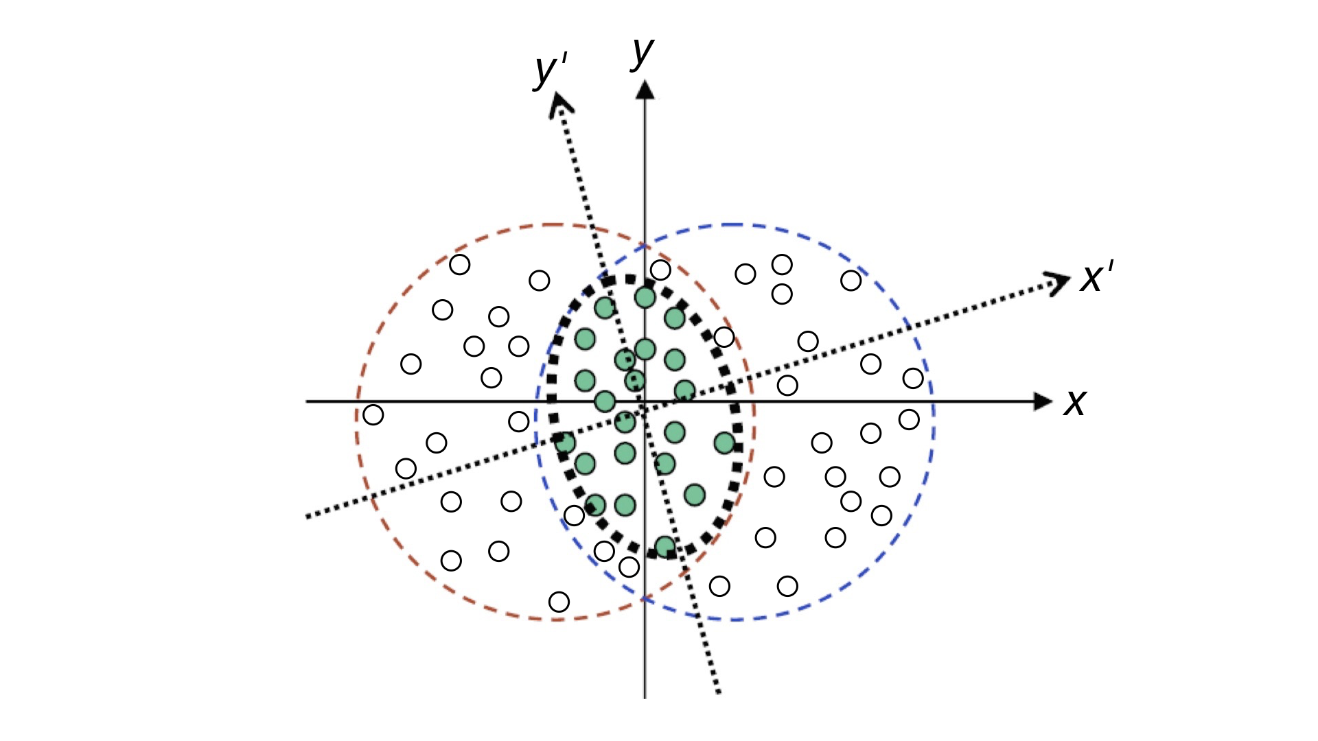
Figure 1: (colour online) Geometry of the collision. Filled circles denote the participants and open circles the spectators. $x^{\prime}$ and $y^{\prime}$ are the principal axes of inertia of the participant zone. Figure adapted from Voloshin:2008dg .

• Reaction Plane (RP): $xz$ plane. It is the plane determined by the impact parameter vector and the beam axis. Orientation of the reaction plane is not directly measurable.

• Participant Plane (PP): $x^{\prime}z^{\prime}$ plane. Same as the RP if there are no initial-state fluctuations. Participant plane is also not directly measurable.

• Event Plane (EP): Estimate of the PP, obtained by measuring the direction of maximum final-state particle density. If there are no fluctuations, EP is an estimate of RP.

It is established by hydrodynamic calculations and is also expected naturally that the initial state of collision governs the final state on an event-by-event basis. In the next two subsections, we describe how the geometries of the initial and final states, in the coordinate and momentum spaces respectively, are captured in terms of a few parameters. One then expects the empirically extracted parameters of the final state (“flow coefficients”) to depend on the theoretically calculated parameters of the initial state (“eccentricities”), in a hopefully simple way.

2.1 Characterization of the initial state

Recall the old definition of the eccentricity $\varepsilon_{2}\equiv\left\langle y^{2}-x^{2}\right\rangle/\left\langle y^{2}+x^{2}\right\rangle$, which is real. In modern parlance, the complex eccentricity vector $\mathcal{E}_{n}$ is defined as Alver:2010gr ; Heinz:2013th

$$\mathcal{E}_{n}\equiv\varepsilon_{n}e^{in\Phi_{n}}\equiv-\frac{\left\langle z^{n}\right\rangle}{\left\langle|z|^{n}\right\rangle}=-\frac{\left\langle r^{n}e^{in\varphi}\right\rangle}{\left\langle r^{n}\right\rangle}=-\frac{\int z^{n}e(z,\tau_{0})r\,dr\,d\varphi}{\int|z|^{n}e(z,\tau_{0})r\,dr\,d\varphi},~{}~{}n\geq 2,$$ (1)

where $\varepsilon_{n}$ is the magnitude and $\Phi_{n}$ determines the phase of the complex vector $\mathcal{E}_{n}$, the complex variable $z\equiv x+iy=re^{i\varphi}$ refers to a point in the transverse or $xy$ plane, $e(z,\tau_{0})$ is the energy (or entropy) density at midrapidity at the initial time $\tau_{0}$, i.e., shortly after the collision and $\left\langle\cdots\right\rangle$ denotes the $e(z,\tau_{0})$-weighted average over the transverse plane in a single event after centering: $\left\langle z\right\rangle=\left\langle re^{i\varphi}\right\rangle=0$. Note that $0\leq\varepsilon_{n}\leq 1$ by definition. $\Phi_{n}$ is called the participant-plane angle in the $n$-th harmonic. $\varepsilon_{n}$ and $\Phi_{n}$ are given by

$$\left.\begin{aligned} \varepsilon_{n}=&\frac{\sqrt{\left\langle r^{n}\cos n\varphi\right\rangle^{2}+\left\langle r^{n}\sin n\varphi\right\rangle^{2}}}{\left\langle r^{n}\right\rangle}\,,\\ \Phi_{n}=&\frac{1}{n}\tan^{-1}\frac{\left\langle r^{n}\sin n\varphi\right\rangle}{\left\langle r^{n}\cos n\varphi\right\rangle}\,,\end{aligned}\right.$$ (2)

modulo $2\pi/n$, because the $n$-th order harmonic has an $n$-fold symmetry in azimuth. It is easy to check that for $n=2$, with $\Phi_{2}$ oriented along the $x$ axis, both Eqs. (1) and (2) yield the old definition of the eccentricity $\varepsilon_{2}\equiv\left\langle y^{2}-x^{2}\right\rangle/\left\langle y^{2}+x^{2}\right\rangle$. Eccentricity $\varepsilon_{n}$ cannot be determined experimentally. However, given a model for the initial state (e.g., Glauber model), $\varepsilon_{n}$ can be calculated from the positions ($r,\varphi$) of the participating nucleons (or partons) in the transverse plane. The magnitude $\varepsilon_{n}$ and the phase $\Phi_{n}$ fluctuate from event to event.

It is sometimes useful to replace the above definition of ${\mathcal{E}}_{n}$ based on moments by a definition based on cumulants, because cumulants subtract off the lower-order correlations and retain only the irreducible correlations Teaney:2013dta . The spatial azimuthal anisotropies then become:

$$\left.\begin{aligned} {\mathcal{E}}_{2}=&-\frac{\left\langle z^{2}\right\rangle}{\left\langle r^{2}\right\rangle}\,,\\ {\mathcal{E}}_{3}=&-\frac{\left\langle z^{3}\right\rangle}{\left\langle r^{3}\right\rangle}\,,\\ {\mathcal{E}}_{4}=&-\frac{1}{\left\langle r^{4}\right\rangle}\left[\left\langle z^{4}\right\rangle-3\left\langle z^{2}\right\rangle^{2}\right]\,,\\ {\mathcal{E}}_{5}=&-\frac{1}{\left\langle r^{5}\right\rangle}\left[\left\langle z^{5}\right\rangle-10\left\langle z^{2}\right\rangle\left\langle z^{3}\right\rangle\right]\,,\\ {\mathcal{E}}_{6}=&-\frac{1}{\left\langle r^{6}\right\rangle}\left[\left\langle z^{6}\right\rangle-15\left\langle z^{4}\right\rangle\left\langle z^{2}\right\rangle-10\left\langle z^{3}\right\rangle^{2}+30\left\langle z^{2}\right\rangle^{3}\right]\,.\end{aligned}\right.$$ (3)

These will be needed later in Sec. 3.3.

Exercise 1: Understand Eqs. (3) in the light of the expressions of cumulants given in Appendix A.

2.2 Characterization of the final state

Anisotropy of the azimuthal distribution of the final-state particles was proposed as a signature of the transverse collective flow in Ref. Ollitrault:1992bk . Characterization of the anisotropy by a Fourier decomposition was proposed in Ref. Voloshin:1994mz . The modern flow picture is a model in which particles in the final state are emitted randomly and independently according to some underlying single-particle probability distribution $P(\phi)$ that fluctuates from event to event Luzum:2011mm :

$$P(\phi)=\frac{1}{2\pi}\sum_{n=-\infty}^{\infty}V_{n}e^{-in\phi}=\frac{1}{2\pi}\sum_{n=-\infty}^{\infty}v_{n}e^{-in(\phi-\Psi_{n})},$$ (4)

where $\phi$ is the azimuthal angle of the momentum of the outgoing particle and $V_{n}$ is a complex Fourier flow coefficient whose magnitude ($v_{n}$) and phase ($\Psi_{n}$) fluctuate from event to event. The angle $\Psi_{n}$ is called the event-plane angle or symmetry-plane angle or reference angle for harmonic $n$. It is easy to check that

$$V_{n}\equiv v_{n}\exp(in\Psi_{n})=\left\langle\exp(in\phi)\right\rangle,$$ (5)

where $\left\langle\cdots\right\rangle$ denotes an average over the probability density in a single event. As $v_{n}$ is real, this also means $v_{n}=\left\langle\cos n(\phi-\Psi_{n})\right\rangle$ and $\left\langle\sin n(\phi-\Psi_{n})\right\rangle=0$. The sine term vanishes because of the symmetry with respect to the event plane. The event-plane angle $\Psi_{n}$ can be determined using Eq. (5):

$$\Psi_{n}=\frac{1}{n}\tan^{-1}\frac{\left\langle\sin n\phi\right\rangle}{\left\langle\cos n\phi\right\rangle},~{}~{}~{}(\rm modulo~{}2\pi/n).$$ (6)

Experimentally, the flow vector $Q_{n}$ defined as $Q_{n}\equiv\sum_{i}w_{i}\exp(in\phi_{i})/\sum_{i}w_{i}$ provides an estimate of the vector $V_{n}$. Here $\phi_{i}$ are the azimuthal angles of the momenta of the detected particles and $w_{i}$ are the weights that are generally inserted to optimize the estimate by accounting for detector nonuniformity and tracking inefficiency. Experimentally, $\Psi_{n}$ is estimated as Poskanzer:1998yz :

$$\Psi_{n}=\frac{1}{n}\tan^{-1}\frac{\sum_{i}w_{i}\sin n\phi_{i}}{\sum_{i}w_{i}\cos n\phi_{i}},~{}~{}~{}(\rm modulo~{}2\pi/n).$$ (7)

Exercise 2: Recall that the event plane is an estimate of the participant plane. Because the number of particles emitted in an event is finite, the event-plane angle $\Psi_{n}$ determined from Eq. (7) fluctuates from event to event around the participant-plane angle $\Phi_{n}$. Hence the true flow $v_{n}$ would differ from the observed flow $v_{n}^{\rm obs}$. Show that $v_{n}=v_{n}^{\rm obs}/R_{n}$, where the ‘resolution factor’ $R_{n}$ is given by $R_{n}=\left\langle\cos n(\Psi_{n}-\Phi_{n})\right\rangle<1$ Ollitrault:1997di .

Defining $V_{-n}=V_{n}^{*}$ (equivalently, $v_{n}=v_{-n}$, $\Psi_{n}=\Psi_{-n}$) and using $V_{0}=v_{0}=1$, one can write $P(\phi)$ also as

$$P(\phi)=\frac{1}{2\pi}\left(1+2\sum_{n=1}^{\infty}v_{n}\cos n(\phi-\Psi_{n})\right),$$ (8)

which is real. As a result, in the final state, the azimuthal distribution of particles that fluctuates event to event is

$$\frac{dN}{d\phi}=\frac{N}{2\pi}\left(1+2\sum_{n=1}^{\infty}v_{n}\cos n(\phi-\Psi_{n})\right).$$ (9)

The angle-independent leading term is called the radial flow. The coefficients $v_{n}$ parametrize the momentum anisotropy of the final-state particle yield. They go by the names directed or dipolar ($n=1$), elliptic ($n=2$), triangular ($n=3$), quadrangular ($n=4$), pentagonal ($n=5$), $\cdots$ flows. Recently, ALICE collaboration has presented results on flow harmonics up to $n=9$ Acharya:2020taj .

In general, $v_{n}$ and $\Psi_{n}$ depend on the transverse momentum $(p_{T})$ and pseudorapidity $(\eta)$. Thus the event-plane angle is not a unique angle for the entire event. It is so only for nonfluctuating smooth initial conditions. The $p_{T}$ dependence of $\Psi_{n}$ may arise due to differently-oriented and different-sized hot spots in the transverse plane emitting particles in different directions with different $\left\langle p_{T}\right\rangle$ Khachatryan:2015oea . The $\eta$ dependence of $\Psi_{n}$ may arise due to a fireball that is twisted or torqued in the longitudinal direction Bozek:2010vz .

Note that the $\varepsilon_{n}$ coefficients characterize the various shape components of the fluctuating initial profile in the coordinate space, just as the $v_{n}$ coefficients characterize those of the fluctuating final state in the momentum space.

2.3 Flow measurements

Theoretically,

$$V_{n}(p_{T},\eta)\equiv v_{n}e^{in\Psi_{n}}(p_{T},\eta)=\frac{\int d\phi e^{in\phi}\frac{dN}{p_{T}dp_{T}d\eta d\phi}}{\int d\phi\frac{dN}{p_{T}dp_{T}d\eta d\phi}}=\left\langle e^{in\phi}\right\rangle,$$ (10)

where $dN/p_{T}dp_{T}d\eta d\phi$ is the particle distribution — usually charged hadron distribution — in an event. $V_{n}(p_{T})$ and $V_{n}(\eta)$ can be defined similarly, by carrying out integrations over $\eta$ or $p_{T}$, respectively, over appropriate ranges, besides the integration over $\phi$. Fully integrated flow $V_{n}$ results from the integration over both $p_{T}$ and $\eta$.

Since the orientations of the reaction plane and the participant plane are unknown, flow $v_{n}$ is usually measured experimentally from event-averaged azimuthal correlations between outgoing particles. Determination of the flow coefficients using multiparticle correlations proceeds as follows. Two-, four-. six- and eight-particle azimuthal correlations are defined as

$$\left.\begin{aligned} \langle\langle 2\rangle\rangle&=\langle\langle e^{in(\phi_{1}-\phi_{2})}\rangle\rangle,\\ \langle\langle 4\rangle\rangle&=\langle\langle e^{in(\phi_{1}+\phi_{2}-\phi_{3}-\phi_{4})}\rangle\rangle,\\ \langle\langle 6\rangle\rangle&=\langle\langle e^{in(\phi_{1}+\phi_{2}+\phi_{3}-\phi_{4}-\phi_{5}-\phi_{6})}\rangle\rangle,\\ \langle\langle 8\rangle\rangle&=\langle\langle e^{in(\phi_{1}+\phi_{2}+\phi_{3}+\phi_{4}-\phi_{5}-\phi_{6}-\phi_{7}-\phi_{8})}\rangle\rangle,\end{aligned}\right.$$ (11)

where $\langle\langle\cdots\rangle\rangle$ denotes averaging over all multiplets in a single collision event and then over all events in a given centrality class. Note that all these ‘observables’ are invariant under rotation in the azimuthal plane, as they should be. (As a counterexample, consider $\langle\langle e^{in(\phi_{1}+\phi_{2}-\phi_{3})}\rangle\rangle$. To make it invariant, we may replace $\phi_{3}$ by $2\phi_{3}$, which, however, mixes harmonics $n$ and $2n$. Mixed-harmonic observables will be discussed in Sec. 3.) Multiparticle cumulants are defined as Borghini:2001vi

$$\left.\begin{aligned} c_{n}\{2\}&=\langle\langle 2\rangle\rangle,\\ c_{n}\{4\}&=\langle\langle 4\rangle\rangle-2\langle\langle 2\rangle\rangle^{2},\\ c_{n}\{6\}&=\langle\langle 6\rangle\rangle-9\langle\langle 2\rangle\rangle\langle\langle 4\rangle\rangle+12\langle\langle 2\rangle\rangle^{3},\\ c_{n}\{8\}&=\langle\langle 8\rangle\rangle-16\langle\langle 2\rangle\rangle\langle\langle 6\rangle\rangle-18\langle\langle 4\rangle\rangle^{2}+144\langle\langle 2\rangle\rangle^{2}\langle\langle 4\rangle\rangle-144\langle\langle 2\rangle\rangle^{4}.\end{aligned}\right.$$ (12)

Exercise 3: Understand Eqs. (12) in the light of the definitions of cumulants given in Eq. (B2) of Appendix B.

The two-particle correlation can be rewritten as

$$\left.\begin{aligned} \langle\langle 2\rangle\rangle=&\langle\langle e^{in(\phi_{1}-\phi_{2})}\rangle\rangle=\langle\langle e^{in(\phi_{1}-\Psi_{n})}e^{-in(\phi_{2}-\Psi_{n})}\rangle\rangle\\ =&\langle\langle e^{in(\phi_{1}-\Psi_{n})}\rangle\langle e^{-in(\phi_{2}-\Psi_{n})}\rangle\rangle=\left\langle v_{n}^{2}\right\rangle,\end{aligned}\right.$$ (13)

where in the first line we assumed that $\Psi_{n}$ is a global phase angle for all the particles selected for averaging, and in the second line we assumed that there are no nonflow correlations, or equivalently, that the angles $(\phi_{1}-\Psi_{n})$ and $(\phi_{2}-\Psi_{n})$ are statistically independent. Note that any dependence on the symmetry plane is eliminated by construction. The higher-order correlations $\langle\langle 4\rangle\rangle$, $\langle\langle 6\rangle\rangle$ and $\langle\langle 8\rangle\rangle$ can be treated similarly. Thus the multiparticle cumulants take the form:

$$\left.\begin{aligned} c_{n}\{2\}&=\langle v_{n}^{2}\rangle,\\ c_{n}\{4\}&=\langle v_{n}^{4}\rangle-2\langle v_{n}^{2}\rangle^{2},\\ c_{n}\{6\}&=\langle v_{n}^{6}\rangle-9\langle v_{n}^{2}\rangle\langle v_{n}^{4}\rangle+12\langle v_{n}^{2}\rangle^{3},\\ c_{n}\{8\}&=\langle v_{n}^{8}\rangle-16\langle v_{n}^{2}\rangle\langle v_{n}^{6}\rangle-18\langle v_{n}^{4}\rangle^{2}+144\langle v_{n}^{2}\rangle^{2}\langle v_{n}^{4}\rangle-144\langle v_{n}^{2}\rangle^{4}.\end{aligned}\right.$$ (14)

Finally, the flow coefficients are given by

$$\left.\begin{aligned} v_{n}\{2\}&=\sqrt{c_{n}\{2\}}=\sqrt{\langle v_{n}^{2}\rangle},\\ v_{n}\{4\}&=\sqrt[4]{-c_{n}\{4\}}=\sqrt[4]{2\langle v_{n}^{2}\rangle^{2}-\langle v_{n}^{4}\rangle},\\ v_{n}\{6\}&=\sqrt[6]{\frac{1}{4}c_{n}\{6\}}=\sqrt[6]{\frac{1}{4}(\langle v_{n}^{6}\rangle-9\langle v_{n}^{2}\rangle\langle v_{n}^{4}\rangle+12\langle v_{n}^{2}\rangle^{3}}),\\ v_{n}\{8\}&=\sqrt[8]{-\frac{1}{33}c_{n}\{8\}}\\ &=\sqrt[8]{-\frac{1}{33}(\langle v_{n}^{8}\rangle-16\langle v_{n}^{2}\rangle\langle v_{n}^{6}\rangle-18\langle v_{n}^{4}\rangle^{2}+144\langle v_{n}^{2}\rangle^{2}\langle v_{n}^{4}\rangle-144\langle v_{n}^{2}\rangle^{4}}).\end{aligned}\right.$$ (15)

The coefficients $-1$, 1/4 and $-1/33$ appearing in front of $c_{n}\{4\}$, $c_{n}\{6\}$ and $c_{n}\{8\}$, respectively, in Eqs. (15), can be understood as follows: If the magnitude of the flow vector does not fluctuate event-to-event, then $\left\langle v_{n}^{k}\right\rangle=v_{n}^{k}$, and it is clear from Eq. (14) that $c_{n}\{2\}=v_{n}^{2}(>0)$, $c_{n}\{4\}=-v_{n}^{4}(<0)$, $c_{n}\{6\}=4v_{n}^{6}(>0)$, $c_{n}\{8\}=-33v_{n}^{8}(<0)$. These when substituted in Eq. (15) ensure that $v_{n}\{2\}=v_{n}\{4\}=v_{n}\{6\}=v_{n}\{8\}=v_{n}$, as expected. An advantage of multiparticle cumulants $v_{n}\{m\}$ is that they suppress nonflow contribution.

For the sake of completeness, we present the inverse of Eqs. (15):

$$\left.\begin{aligned} \langle v_{n}^{2}\rangle&=v_{n}\{2\}^{2},\\ \langle v_{n}^{4}\rangle&=-v_{n}\{4\}^{4}+2v_{n}\{2\}^{4},\\ \langle v_{n}^{6}\rangle&=4v_{n}\{6\}^{6}-9v_{n}\{2\}^{2}\,v_{n}\{4\}^{4}+6v_{n}\{2\}^{6},\\ \langle v_{n}^{8}\rangle&=-33v_{n}\{8\}^{8}+64v_{n}\{6\}^{6}\,v_{n}\{2\}^{2}+18v_{n}\{4\}^{8}-72v_{n}\{2\}^{4}\,v_{n}\{4\}^{4}+24v_{n}\{2\}^{8}.\end{aligned}\right.$$ (16)

The flow coefficients in Eq. (15) are driven by the corresponding initial-state eccentricities defined as Bhalerao:2006tp :

$$\left.\begin{aligned} \varepsilon_{n}\{2\}&=\sqrt{\langle\varepsilon_{n}^{2}\rangle},\\ \varepsilon_{n}\{4\}&=\sqrt[4]{2\langle\varepsilon_{n}^{2}\rangle^{2}-\langle\varepsilon_{n}^{4}\rangle},\\ \varepsilon_{n}\{6\}&=\sqrt[6]{\frac{1}{4}(\langle\varepsilon_{n}^{6}\rangle-9\langle\varepsilon_{n}^{2}\rangle\langle\varepsilon_{n}^{4}\rangle+12\langle\varepsilon_{n}^{2}\rangle^{3}}),\\ \varepsilon_{n}\{8\}&=\sqrt[8]{-\frac{1}{33}(\langle\varepsilon_{n}^{8}\rangle-16\langle\varepsilon_{n}^{2}\rangle\langle\varepsilon_{n}^{6}\rangle-18\langle\varepsilon_{n}^{4}\rangle^{2}+144\langle\varepsilon_{n}^{2}\rangle^{2}\langle\varepsilon_{n}^{4}\rangle-144\langle\varepsilon_{n}^{2}\rangle^{4}}).\end{aligned}\right.$$ (17)

Consider $V_{2}=v_{2}\exp(i\,2\,\Psi_{2}),\,V_{4}=v_{4}\exp(i\,4\,\Psi_{4})$ and $V_{6}=v_{6}\exp(i\,6\,\Psi_{6})$. In the foregoing discussion, we implicitly assumed that $V_{4}$ and $V_{6}$ are to be analysed with respect to their respective reference angles, $\Psi_{4}$ and $\Psi_{6}$. But that is not necessary. We could alternately analyse $V_{4}$ with respect to the direction of $\Psi_{2}$, leading to $\exp(i4(\Psi_{4}-\Psi_{2}))$. Similarly, analysing $V_{6}$ with respect to the direction of $\Psi_{2}$ or of $\Psi_{3}$ would involve $\exp(i6(\Psi_{6}-\Psi_{2}))$ or $\exp(i6(\Psi_{6}-\Psi_{3}))$. We shall encounter such quantities later when we discuss event-plane correlators (Sec. 3.2).

For recent theoretical developments about calculating and analyzing multiparticle cumulants to arbitrary order, see DiFrancesco:2016srj ; Moravcova:2020wnf .

2.4 Probability density function (PDF)

As stated above, the flow magnitude ($v_{n}$) and phase ($\Psi_{n}$) (or equivalently, $x$ and $y$ components of $V_{n}$) fluctuate event to event. The probability density function $P(v_{n})$ has been measured. Figure 2 shows the ATLAS data on $P(v_{2}),\,P(v_{3})$ and $P(v_{4})$ for various centrality bins at $\sqrt{s_{\rm NN}}=2.76$ TeV Aad:2013xma . As one goes from central to peripheral collisions, the distributions broaden reflecting the gradual increase of $v_{n}$ with centrality. Centrality dependence of $P(v_{2})$ is stronger than that of $P(v_{3})$ and $P(v_{4})$, because $\varepsilon_{2}$ which drives $v_{2}$ changes more dramatically from central to peripheral collisions than do $\varepsilon_{3}$ and $\varepsilon_{4}$. Similar results were reported by ALICE at $\sqrt{s_{\rm NN}}=5.02$ TeV Acharya:2018lmh . Flow fluctuations affect two- and multiparticle cumulants in different ways (Exercise 4).

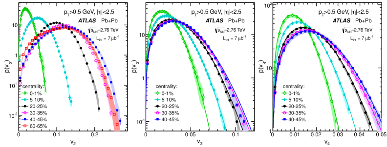
Figure 2: (colour online) ATLAS data on probability density function $P(v_{n})$ in several centrality intervals for n = 2 (left panel), n = 3 (middle panel) and n = 4 (right panel) Aad:2013xma .

Exercise 4: Define $\sigma_{v}^{2}\equiv\left\langle v^{2}\right\rangle-\left\langle v\right\rangle^{2}$. (Harmonic index $n$ is suppressed for simplicity of notation.) Note that $v\{2\}$, $v\{4\}$ and $v\{6\}$ defined in Eq. (15) are various functions of $v$, denoted generically by $f(v)$. Taylor expand $f(v)$ around the mean flow $\left\langle v\right\rangle$ to the second order and take the mean to get $\left\langle f(v)\right\rangle=f(\left\langle v\right\rangle)+\sigma_{v}^{2}f^{\prime\prime}(\left\langle v\right\rangle)/2$. Show that, $v\{2\}^{2}=\left\langle v\right\rangle^{2}+\sigma_{v}^{2}$ and $v\{4\}^{2}\approx\left\langle v\right\rangle^{2}-\sigma_{v}^{2}\approx v\{6\}^{2}$, and hence $v\{2\}\approx\left\langle v\right\rangle+\sigma_{v}^{2}/(2\left\langle v\right\rangle)$ and $v\{4\}\approx\left\langle v\right\rangle-\sigma_{v}^{2}/(2\left\langle v\right\rangle)\approx v\{6\}$. Thus $v\{2\}>\left\langle v\right\rangle>v\{4\}\approx v\{6\}$. In other words, fluctuations, in general, tend to enhance $v\{2\}$ and suppress $v\{4\}$, $v\{6\}$ compared to $\left\langle v\right\rangle$ Voloshin:2008dg ; Ollitrault:2009ie . (N.B. Here, we did not assume the fluctuations to be Gaussian.)

As a measure of the relative flow fluctuations, one defines:

$$F(v_{n})\equiv\sqrt{\frac{v_{n}\{2\}^{2}-v_{n}\{4\}^{2}}{v_{n}\{2\}^{2}+v_{n}\{4\}^{2}}}=\frac{\sigma_{v_{n}}}{\left\langle v_{n}\right\rangle},$$ (18)

where the last equality follows from Exercise 4. Note that Eq. (18) is based on two assumptions: (a) there are no nonflow correlations in $v_{n}\{2\}$ and $v_{n}\{4\}$, and (b) $\sigma_{v_{n}}\ll\left\langle v_{n}\right\rangle$.

Flow coefficients $v_{n}\{m\},m=2,4,6,8$ have also been measured. Consider first $n=2$. Figure 3 shows the CMS data Sirunyan:2017fts on $v_{2}\{m\}$ for $m=2,4,6,8$. Evidently, $v_{2}\{2\}>v_{2}\{4\}\approx v_{2}\{6\}\approx v_{2}\{8\}$. It is easy to understand this feature of the data by making a simple Gaussian ansatz Voloshin:2007pc for the fluctuations of the vector $V_{n}$ in the transverse ($xy$) plane. Denoting $x$ and $y$ components of $V_{2}$ by $v_{x}$ and $v_{y}$ for simplicity of notation, one assumes the probability distribution to be

$$P(v_{x},v_{y})=\frac{1}{2\pi\sigma^{2}}\exp\left(-\frac{(v_{x}-{\bar{v}})^{2}+v_{y}^{2}}{2\sigma^{2}}\right),$$ (19)

where $\bar{v}=\left\langle v_{x}\right\rangle$, $\left\langle v_{y}\right\rangle=0$ and $\sigma^{2}=\sigma_{x}^{2}=\sigma_{y}^{2}$ is the variance of the Gaussian distribution. Assume further that $v_{x}$ and $v_{y}$ are uncorrelated.

Exercise 5: Using Eqs. (15) and (19) and the moments of the Gaussian distribution given in Table 1 in Appendix C, show that $v_{2}\{2\}=\sqrt{{\bar{v}}^{2}+2\sigma^{2}}$ and $v_{2}\{4\}=v_{2}\{6\}=v_{2}\{8\}={\bar{v}}$. This shows that the data in Fig. 3 is consistent with the Gaussian ansatz Voloshin:2007pc .

A more careful inspection of the data, however, shows that there are small differences in the magnitudes of $v_{2}\{4\}$, $v_{2}\{6\}$ and $v_{2}\{8\}$, indicating non-Gaussian fluctuations in the data on $v_{2}$ (Fig. 4).

We next turn to $n=3$. Unlike $v_{2}$, which can be nonzero even in the absence of fluctuations, $v_{3}$ (at midrapidity) arises only due to fluctuations. So the Gaussian ansatz for $v_{3}$ is

$$P(v_{x},v_{y})=\frac{1}{2\pi\sigma^{2}}\exp\left(-\frac{v_{x}^{2}+v_{y}^{2}}{2\sigma^{2}}\right).$$ (20)

Exercise 6: Using Eqs. (15) and (20) and the moments of the Gaussian distribution given in Table 1 in Appendix C, show that $v_{3}\{2\}=\sqrt{2}\sigma$ and $v_{3}\{4\}=v_{3}\{6\}=v_{3}\{8\}=0$.

Figure 5 shows ATLAS results for

$$nc_{n}\{4\}\equiv\frac{c_{n}\{4\}}{c_{n}\{2\}^{2}}=-\frac{v_{n}\{4\}^{4}}{v_{n}\{2\}^{4}}=\frac{\left\langle v_{n}^{4}\right\rangle}{\left\langle v_{n}^{2}\right\rangle^{2}}-2,$$ (21)

for $n=3$. It is clear from the figure that $v_{3}\{4\}\neq 0$, except for the most central collisions. This is an evidence for non-Gaussianity in the triangular flow fluctuations. Note that $\left\langle v_{n}^{4}\right\rangle/\left\langle v_{n}^{2}\right\rangle^{2}-2$ occurring in Eq. (21) is a measure of excess kurtosis; see the discussion of $f(r)$ in Appendix C.

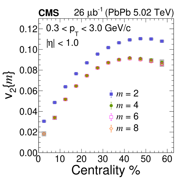
Figure 3: (colour online) Note that $v_{2}\{2\}>v_{2}\{4\}\approx v_{2}\{6\}\approx v_{2}\{8\}$. This is consistent with the Gaussian ansatz Voloshin:2007pc ; see Exercise 5. Figure from Sirunyan:2017fts .

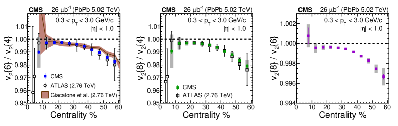
Figure 4: (colour online) Note the small differences in the magnitudes of $v_{2}\{4\}$, $v_{2}\{6\}$ and $v_{2}\{8\}$. This is the evidence for non-Gaussianity in the elliptic flow fluctuations. Figure from Sirunyan:2017fts .

Figure 5: (colour online) $nc_{3}\{4\}\equiv-v_{3}\{4\}^{4}/v_{3}\{2\}^{4}$. Data points with various colours correspond to different $p_{T}$ ranges. Note the nonzero value of $v_{3}\{4\}$. This is the evidence for non-Gaussianity in the triangular flow fluctuations; see Exercise 6. Figure from Aaboud:2019sma .

Exercise 7: Recall that the cumulants (Eq. (14)) are functions of even moments of the distribution of $v_{n}$. For $n=2$ (the most central collisions only) and $n=3$ (all centralities), flow is solely due to fluctuations. If the statistics of these fluctuations is a 2-dimensional Gaussian (Appendix C), then show that the scaled even moments $m_{n}^{(k)}$ satisfy: $$m_{n}^{(k)}\equiv\frac{\left\langle v_{n}^{2k}\right\rangle}{\left\langle v_{n}^{2(k-1)}\right\rangle\left\langle v_{n}^{2}\right\rangle}=k,~{}~{}~{}~{}~{}(k=2,3,4).$$ These expectations are borne out quite well in AMPT model calculations Bhalerao:2014xra .

If the flow fluctuations are not Gaussian, then what is the right underlying PDF? A related question is what is the PDF for the fluctuating initial eccentricity? This issue has been discussed in the literature: A distribution that was proposed early on was the Bessel-Gaussian distribution Voloshin:2007pc . It worked well for central collisions, but not so well for peripheral collisions. A new parametrization named the Elliptic Power distribution, for the PDF of the initial eccentricity at a fixed centrality, was proposed in Ref. Yan:2014afa . Unlike the Bessel-Gaussian distribution, this fits several Monte Carlo models of the initial state for all centralities.

For more recent works that probe the skewness and kurtosis of the non-Gaussian fluctuations in heavy-ion collisions, see Giacalone:2016eyu ; Bhalerao:2018anl . In cosmology, the primordial non-Gaussianity is consistent with zero, and the present-day non-Gaussianity is the result of the evolution of the universe. In heavy-ion collisions, on the other hand, the primordial non-Gaussianity is sizable, and it is partially washed out as a result of the system evolution Bhalerao:2019fzp . Future high-statistics measurements of kurtosis of elliptic flow fluctuations would provide deeper insights into the hydrodynamic behaviour and the equation of state of quark-gluon plasma.

We discussed in this section the probability density function $P(v_{n})$. Ideally, one would like to measure the full probability density function $P(V_{1},V_{2},\cdots,V_{n})=\\ P(v_{1},v_{2},\cdots,v_{n},\Psi_{1},\Psi_{2},\cdots,\Psi_{n})$. We are far from that goal.

2.5 Ridge

Equation (9) is the Fourier expansion of the single-particle distribution in the azimuthal plane. Fourier expansion of the two-particle distribution is similarly given by

$$\frac{dN^{\rm pair}}{d\Delta\phi}=\frac{N^{\rm pair}}{2\pi}\left(1+2\sum_{n=1}^{\infty}V_{n\Delta}\cos n\Delta\phi\right),$$ (22)

where $\Delta\phi=\phi_{1}-\phi_{2}$ and $V_{n\Delta}=\left\langle\exp(in\Delta\phi)\right\rangle$ are the two-particle Fourier coefficients which fluctuate from event to event. One can similarly define $d^{2}N^{\rm pair}/d\Delta\eta\,d\Delta\phi$, where $\Delta\eta=\eta_{1}-\eta_{2}$. This quantity is displayed in Figs. 6 and 7.

Figure 6 shows two-charged-particle correlations as a function of $\Delta\eta$ and $\Delta\phi$, measured by CMS Chatrchyan:2013nka , in PbPb and pPb collisions. The sharp near-side ($\Delta\phi\approx 0$) peak at $\Delta\eta\approx 0$ is the signature of short-range correlations arising due to jet fragmentation. Ignoring this, the striking long-range (large $\Delta\eta$) wave-like structure that we see on the near-side is called the ridge. It indicates that particles widely separated in pseudorapidity experience a collective push in the same azimuthal direction. Production of a small drop of fluid is a natural explanation of such a correlation present at all rapidities. The peaking around $\Delta\phi=0$ and $\pi$ is the signature of the dominant elliptic flow ($v_{2}$) with some admixture of other harmonics notably $v_{3}$ (see Exercise 8). Thus not only the flow harmonics $v_{n}$, but even the correlations observed between particles separated by a large pseudorapidity gap could be explained by a collective behaviour. Causality requires that the long-range structure seen in the ridge originates in the earliest stages of the collision when the transverse geometry is almost rapidity independent Dumitru:2008wn .

Exercise 8: Make three different plots of $\cos(2\Delta\phi)$, $\cos(2\Delta\phi)+0.25\cos(3\Delta\phi)$ and $\cos(2\Delta\phi)+0.55\cos(3\Delta\phi)$, in the range $\Delta\phi=-3\pi/2$ to $\pi/2$. Notice how the heights and widths of the two peaks change as one increases the admixture of $v_{3}$. Notice also the appearance of a “shoulder” in the away-side peak. Compare with Fig. 5 of CMS:2013bza which is similar to our Fig. 6(a), but for ultracentral (0-0.2 %) collisions, and clearly shows the shoulder formation on the away side.

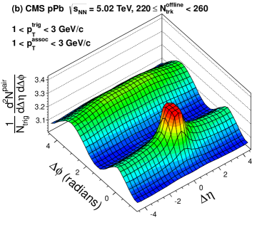
Figure 6: (colour online) Two-charged-particle correlations in (a) PbPb and (b) pPb collisions observed by CMS Chatrchyan:2013nka . Semiperipheral PbPb collisions are selected so that particle multiplicities are similar to those in the pPb case. In (b), the sharp near-side peak from jet correlations is truncated to emphasize the structure outside that region.

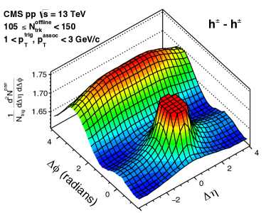
Figure 7: (colour online) Two-charged-particle correlations in (left) low-multiplicity (10-20) and (right) high-multiplicity (105-150) pp collisions observed by CMS Khachatryan:2016txc .

Interestingly, the ridge is also observed in high-multiplicity pp collisions (Fig. 7). This begs the question: is quark-gluon plasma formed or is hydrodynamic flow developed also in high-multiplicity pp (and p-nucleus) collisions? This issue is still being debated (see Sec. 4).

2.6 Flow decorrelation and factorization breaking

Consider the two-particle Fourier coefficient $V_{n\Delta}=\left\langle\exp(in\Delta\phi)\right\rangle$ occurring in Eq. (22). Making the same assumptions as in the derivation of Eq. (13), one gets $V_{n\Delta}=v_{n}^{2}$. However, as stated in Sec. 2.2, the event-plane angle $\Psi_{n}$ may depend on the transverse momentum $(p_{T})$ and pseudorapidity $(\eta)$, and hence may not be the same in the two bins $a$ and $b$ from which the two particles are taken. In this case, $V_{n\Delta}$ in a single event is given by

$$\left.\begin{aligned} V_{n\Delta}(a,b)=\left\langle e^{in(\phi^{a}-\phi^{b})}\right\rangle=\left\langle e^{in\phi^{a}}\right\rangle\left\langle e^{-in\phi^{b}}\right\rangle=V_{n,a}V_{n,b}^{*}=v_{n,a}v_{n,b}\,e^{in(\Psi_{n}^{a}-\Psi_{n}^{b})},\end{aligned}\right.$$

where $\left\langle\cdots\right\rangle$ denotes the average over one event and the second equality is obtained by assuming that there are no nonflow correlations. Factorization (of two-particle correlations) refers to $V_{n\Delta}(a,b)$ getting factorized into a product of single-particle harmonics, $v_{n,a}$ and $v_{n,b}$: $V_{n\Delta}(a,b)=v_{n,a}\times v_{n,b}$. Factorization breaks down ($V_{n\Delta}(a,b)\neq v_{n,a}\times v_{n,b}$) if $\Psi_{n}$ is not the same in the two bins and/or if there are nonflow correlations. The latter effect can be minimized by introducing a large-enough pseudorapidity gap between the two bins.

Experimentally, one further averages over many events to write

$$\left.\begin{aligned} V_{n\Delta}(a,b)=\left\langle V_{n,a}V_{n,b}^{*}\right\rangle=\left\langle v_{n,a}v_{n,b}\,e^{in(\Psi_{n}^{a}-\Psi_{n}^{b})}\right\rangle,\end{aligned}\right.$$ (23)

where $\left\langle\cdots\right\rangle$ denotes the average over many events. Factorization ratio $r_{n}(p_{T}^{a},p_{T}^{b})$ is defined as Gardim:2012im

$$r_{n}(p_{T}^{a},p_{T}^{b})\equiv\frac{V_{n\Delta}(p_{T}^{a},p_{T}^{b})}{\sqrt{V_{n\Delta}(p_{T}^{a},p_{T}^{a})V_{n\Delta}(p_{T}^{b},p_{T}^{b})}}=\frac{\left\langle v_{n}(p_{T}^{a})v_{n}(p_{T}^{b})\cos n(\Psi_{n}(p_{T}^{a})-\Psi_{n}(p_{T}^{b}))\right\rangle}{\sqrt{\left\langle v_{n}^{2}(p_{T}^{a})\right\rangle\left\langle v_{n}^{2}(p_{T}^{b})\right\rangle}}.$$ (24)

It measures the flow decorrelation between momentum bins, i.e., $p_{T}$-dependent event-plane angle fluctuations. If $V_{n\Delta}$ factorizes, $r_{n}$ is obviously unity, otherwise it is less than unity by the Cauchy–-Schwarz inequality. In the most central events initial-state fluctuations play a dominant role, and so $r_{n}$ deviates from unity significantly. $r_{n}(p_{T}^{a},p_{T}^{b})$ is a sensitive discriminator of the models of the initial-state geometry in the transverse plane. Specifically, it could probe the granularity or spatial extent of the density fluctuations in the transverse plane in the initial state.

Assuming $V_{n\Delta}(p_{T}^{a},p_{T}^{b})$ factorizes into the product of single-particle anisotropies, $p_{T}$ dependence of the latter can be determined experimentally from

$$v_{n}(p_{T}^{a})=\frac{V_{n\Delta}(p_{T}^{a},p_{T}^{b})}{\sqrt{V_{n\Delta}(p_{T}^{b},p_{T}^{b})}},$$ (25)

where the reference momentum $p_{T}^{b}$ is chosen not too large to minimize correlations from jets at higher $p_{T}$.

The longitudinal decorrelation or $\eta$-dependent factorization breakdown cannot be studied by simply replacing $p_{T}^{a}$ and $p_{T}^{b}$ in Eq. (24) by $\eta_{a}$ and $\eta_{b}$, respectively, because the denominator would be badly contaminated by short-range nonflow correlations. Instead, one defines the following observable:

$$\left.\begin{aligned} r_{n}(\eta)&\equiv\frac{\left\langle V_{n}(-\eta)V_{n}^{*}(\eta_{ref})\right\rangle}{\left\langle V_{n}(+\eta)V_{n}^{*}(\eta_{\rm ref})\right\rangle}\\ &=\frac{\left\langle v_{n}(-\eta)v_{n}(\eta_{\rm ref})\cos n(\Psi_{n}(-\eta)-\Psi_{n}(\eta_{\rm ref}))\right\rangle}{\left\langle v_{n}(+\eta)v_{n}(\eta_{\rm ref})\cos n(\Psi_{n}(+\eta)-\Psi_{n}(\eta_{\rm ref}))\right\rangle},\end{aligned}\right.$$ (26)

with a large gap between $\eta$ and $\eta_{\rm ref}$. Experimentally, it is found that $v_{n}$ and $\Psi_{n}$ fluctuate along the longitudinal direction, even in a given event Khachatryan:2015oea ; Aaboud:2017tql . $r_{n}(\eta)$ is unity at $\eta=0$ and decreases as $\eta$ increases Aad:2020gfz . Hydrodynamic model calculations show that $r_{n}(\eta)$ is driven mostly by the longitudinal structure of the primordial state. The study of $r_{n}(\eta)$ puts constraints on the complete three-dimensional modelling of the initial state used in 3+1D models of the system evolution. A significant breakdown of factorization in $\eta$ is also observed in pPb collisions Khachatryan:2015oea .

To conclude, experimentally, factorization breakdown or flow decorrelation has been observed as a function of both $p_{T}$ and $\eta$ Khachatryan:2015oea ; CMS:2013bza ; Aaboud:2017tql . For $v_{2}$ in central PbPb collisions at LHC the effect can be as large as 20%.

3 Observables with Mixed Harmonics

Flow observables discussed so far referred to a single harmonic $n$. We now discuss flow observables with mixed harmonics. These provide new handles on the initial state as well as the properties of the medium. Specifically, they can discriminate among the various initial-state models as well as among different parametrizations of the temperature dependence of the specific shear ($\eta/s$) and bulk viscosity ($\zeta/s$); $s$ is the entropy density.

In Sec. 2.3 we discussed multiparticle correlations involving only a single harmonic ($n$). The most general $k$-particle correlation involving harmonics $n_{1},n_{2},\cdots,n_{k}$ can be written as Bhalerao:2011yg

$$v\{n_{1},n_{2},\cdots,n_{k}\}=\langle\langle e^{i(n_{1}\phi_{1}+\cdots+n_{k}\phi_{k})}\rangle\rangle,$$ (27)

where $n_{1},n_{2},\cdots,n_{k}$ are integers satisfying $n_{1}+n_{2}+\cdots+n_{k}=0$, so that this correlation observable is invariant under rotation in the azimuthal plane. The notation $\langle\langle\cdots\rangle\rangle$ is as in Eq. (11). If there are no nonflow correlations, this becomes

$$v\{n_{1},n_{2},\cdots,n_{k}\}=\langle\langle e^{in_{1}\phi_{1}}\rangle\cdots\langle e^{in_{k}\phi_{k}}\rangle\rangle=\langle v_{n_{1}}\cdots v_{n_{k}}e^{i(n_{1}\Psi_{n_{1}}+\cdots+n_{k}\Psi_{n_{k}})}\rangle,$$ (28)

where in the final expression the average is only over events. Using this, a number of new flow observables were constructed to study mixed correlations between $v_{1},\,v_{2}$ and $v_{3}$ Bhalerao:2011yg ; Bhalerao:2011ry .

3.1 Symmetric cumulants

Symmetric cumulants $SC(m,n)$ and $NSC(m,n)$ measure the correlations between event-by-event fluctuations of the magnitudes of the complex flow vectors $V_{m}$ and $V_{n}$ ($m\neq n$):

$$\left.\begin{aligned} SC(m,n)&\equiv\left\langle v_{m}^{2}v_{n}^{2}\right\rangle-\left\langle v_{m}^{2}\right\rangle\left\langle v_{n}^{2}\right\rangle,\\ NSC(m,n)&\equiv\frac{\left\langle v_{m}^{2}v_{n}^{2}\right\rangle-\left\langle v_{m}^{2}\right\rangle\left\langle v_{n}^{2}\right\rangle}{\left\langle v_{m}^{2}\right\rangle\left\langle v_{n}^{2}\right\rangle},\end{aligned}\right.$$ (29)

which obviously vanish if $v_{m}^{2}$ and $v_{n}^{2}$ are uncorrelated or if there are no flow fluctuations. $NSC(m,n)$ can be looked upon as the mixed kurtosis of $v_{m}$ and $v_{n}$ (see Eq. (A3)). Hydrodynamic calculations show that $v_{n}$ scales approximately linearly with $\varepsilon_{n}$, for $n=2,3$. An advantage in defining the ratio as in Eq. (29) is that the constants of proportionality between $v_{n}$ and $\varepsilon_{n}$ drop out, thereby directly connecting experimental observables with the properties of the initial state. Symmetric cumulant is a four-particle observable.

Exercise 9: Equation (13) together with the discussion following it, explain how $\left\langle v_{n}^{2}\right\rangle$ and $\left\langle v_{n}^{4}\right\rangle$ can be measured. Explain how you would measure $\left\langle v_{m}^{2}v_{n}^{2}\right\rangle$. Note also that, as in Eq. (13), any dependence on the symmetry plane is eliminated by construction.

Figure 8 shows the ALICE results for $SC(4,2)$ and $SC(3,2)$ as a function of centrality. $SC(4,2)$ is found to be positive and $SC(3,2)$ negative. This indicates that if in an event $v_{2}$ is larger than $\left\langle v_{2}\right\rangle$, then there is an enhanced probability of finding $v_{4}$ larger than $\left\langle v_{4}\right\rangle$. Similarly, if in an event $v_{2}$ is larger than $\left\langle v_{2}\right\rangle$, then there is an enhanced probability of finding $v_{3}$ smaller than $\left\langle v_{3}\right\rangle$. In other words, $v_{2}$ and $v_{4}$ are correlated, whereas $v_{2}$ and $v_{3}$ are anticorrelated, for all centralities. The detailed behaviour, however, depends on whether one is in the fluctuation-dominated (most central) regime or the geometry-dominated (midcentral) regime. Figure 8 also shows the HIJING model results which are consistent with zero. Now, this model includes nonflow azimuthal correlations due to jet production, but has no physics of collectivity. Evidently, the nonzero ALICE results cannot be explained by nonflow effects, showing that the symmetric cumulants $SC(m,n)$ are robust against systematic biases originating from nonflow effects. More recently, ALICE have presented data on $SC(4,3)$, $SC(5,2)$ and $SC(5,3)$ Acharya:2017gsw . Interestingly, negative $SC(3,2)$ has been observed also in the highest-multiplicity pp and pPb events Sirunyan:2017uyl ; Acharya:2019vdf .

Recently, the idea of symmetric cumulants was generalized and a new set of observables, which quantify the correlations of flow fluctuations involving more than two flow amplitudes, was introduced Mordasini:2019hut .

Figure 8: (colour online) Centrality dependence of the symmetric cumulants $SC(4,2)$ (red filled squares) and $SC(3,2)$ (blue filled circles). Boxes represent systematical errors. HIJING model results are shown with hollow markers. Figure from ALICE:2016kpq .

3.2 Event-plane correlators

Event-plane correlators or symmetry-plane correlators measure the correlations between event-by-event fluctuations of the phases of the complex flow vectors $V_{m}$ and $V_{n}$ ($m\neq n$). They represent higher-order correlations, involving at least three particles (see below). One can construct two-, three-, or higher-plane correlators. They thus bring in a large number of new observables that provide new, detailed insight into the hydrodynamic response and the initial state.

Suppose we want to construct an observable that measures correlations between the event planes $\Psi_{m}$ and $\Psi_{n}$. Recall first that $\Psi_{l}$ can be determined only modulo $2\pi/l$ (Eq. (6)). Hence the observable should be invariant under $\Psi_{l}\rightarrow\Psi_{l}+2\pi/l$. Moreover, it should also be invariant under a global rotation through an arbitrary angle. An observable that satisfies both these requirements is $\left\langle\cos k(\Psi_{m}-\Psi_{n})\right\rangle$, where $k$ is a common multiple of $m$ and $n$. Consider the simplest example of $\left\langle\cos 4(\Psi_{4}-\Psi_{2})\right\rangle$. In order to measure this correlator, we consider

$$\left.\begin{aligned} \frac{{\rm Re}\left\langle V_{4}V_{2}^{\ast 2}\right\rangle}{\sqrt{\left\langle|V_{4}|^{2}\right\rangle\left\langle|V_{2}|^{4}\right\rangle}}&=\frac{\left\langle v_{4}v_{2}^{2}\cos 4(\Psi_{4}-\Psi_{2})\right\rangle}{\sqrt{\left\langle v_{4}^{2}\right\rangle\left\langle v_{2}^{4}\right\rangle}}\approx\left\langle\cos 4(\Psi_{4}-\Psi_{2})\right\rangle,\end{aligned}\right.$$ (30)

where $V_{n}$ is the experimentally measured flow vector, often denoted by $Q_{n}$ or $q_{n}$ (see Sec. 2.2.). It is clear that the left-hand side of the above equation involves averaging $\exp(2i\phi_{j}+2i\phi_{k}-4i\phi_{l})$ over triplets of particles in an event and then over many events, and thus necessarily involves three-particle correlations. In practice, the three particles are taken from two or more different pseudorapidity bins to minimize the short-range nonflow correlations. Observables for other event-plane correlators can be constructed similarly Bhalerao:2013ina .

Exercise 10: Table I in Ref. Bhalerao:2013ina lists two-, three- and four-plane correlators, along with the total number of particles that are involved in each case. For example, the two-event-plane correlator $\left\langle\cos 12(\Psi_{2}-\Psi_{4})\right\rangle$, the three-event-plane correlator $\left\langle\cos(10\Psi_{2}-6\Psi_{3}-4\Psi_{4})\right\rangle$ and the four-event-plane correlator $\left\langle\cos(6\Psi_{2}+3\Psi_{3}-4\Psi_{4}-5\Psi_{5})\right\rangle$, involve 9, 8 and 6 particles, respectively. Understand this Table.

Figure 9 shows the ATLAS data on eight two-plane correlators as a function of centrality for Pb-Pb collisions at $\sqrt{s_{\rm NN}}=2.76$ TeV Aad:2014fla . Given a model for the initial state, say the Glauber model, one can calculate participant-plane correlators as a function of centrality; these are also shown in Fig. 9. Here the participant-plane correlators and event-plane correlators are being compared with each other to illustrate the role played by the hydrodynamic evolution in converting the initial-state spatial correlations between different harmonics into the corresponding final-state momentum-space correlations. For the most central events, where fluctuations and not geometry is the dominant feature, the two-plane (Fig. 9) as well as three-plane Aad:2014fla correlators vanish (with the sole exception of $\left\langle\cos 6(\Phi_{3}-\Phi_{6})\right\rangle$). For off-central collisions, geometry takes over, and the correlators increase in magnitude. This is similar to the centrality dependence of the symmetric cumulants (Fig. 8). For off-central collisions, the participant-plane correlators and event-plane correlators generally differ significantly, especially for higher harmonics, pointing to the misalignment between $\Psi_{n}$ and $\Phi_{n}$, owing to the contributions of the nonlinear flow modes, to be discussed in the next subsection.

ALICE collaboration has measured a few two- and three-plane correlators; they denote them generically by $\rho_{n,mk}$ Acharya:2020taj ; Acharya:2017zfg . A recent paper has pointed out problems with the current methods of measuring symmetry-plane correlations and has proposed a new estimator as an improvement Bilandzic:2020csw .

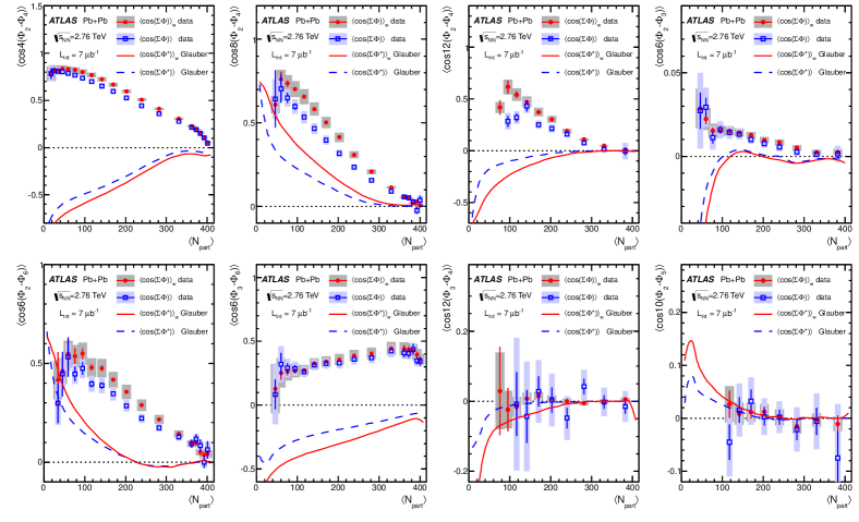
Figure 9: (colour online) ATLAS data Aad:2014fla on two-event-plane correlators as a function of centrality. Red solid symbols and blue open symbols represent two different analysis methods. Red solid and blue dashed curves represent Glauber-model predictions for two-participant-plane correlators using two different methods. Here $\Phi_{n}$ denotes the event-plane and $\Phi_{n}^{*}$ the participant plane, which differs from our convention.

3.3 Nonlinear flow modes and mode coupling or mixing

Hydrodynamic calculations show that $V_{n}$ scales approximately linearly with the initial eccentricity ${\mathcal{E}}_{n}$, for $n=2,3$. For higher harmonics, however, $V_{n}$ receives contributions from eccentricities in the lower harmonics as well Teaney:2012ke . For complex flow vectors $V_{n}\,(n\geq 4)$ one can write the vector sum of the linear and nonlinear response terms as Acharya:2020taj ; Acharya:2017zfg ; Qian:2016fpi .

$$\begin{split}V_{4}&=V_{4\mathrm{L}}+V_{4\mathrm{NL}}=V_{4\mathrm{L}}+\chi_{4,22}V_{2}^{2},\\ V_{5}&=V_{5\mathrm{L}}+V_{5\mathrm{NL}}=V_{5\mathrm{L}}+\chi_{5,23}V_{2}V_{3},\\ V_{6}&=V_{6\mathrm{L}}+V_{6\mathrm{NL}}=V_{6\mathrm{L}}+\chi_{6,222}V_{2}^{3}+\chi_{6,33}V_{3}^{2}+\chi_{6,24}V_{2}V_{4L},\\ V_{7}&=V_{7\mathrm{L}}+V_{7\mathrm{NL}}=V_{7\mathrm{L}}+\chi_{7,223}V_{2}^{2}V_{3}+\chi_{7,34}V_{3}V_{4L}+\chi_{7,25}V_{2}V_{5L},\\ V_{8}&=V_{8\mathrm{L}}+V_{8\mathrm{NL}}=V_{8\mathrm{L}}+\chi_{8,2222}V_{2}^{4}+\chi_{8,233}V_{2}V_{3}^{2}+\mathcal{E}(V_{4L},V_{5L},V_{6L}),\end{split}$$ (31)

where the first term on the right in each equation is called the linear flow mode and the remaining terms constitute the nonlinear flow modes. The (real) coefficients $\chi$ are called the nonlinear flow mode coefficients, and $\mathcal{E}(\cdots)$ in the last equation denotes the remaining terms in $V_{8}$.

Now, suppose the linear terms $V_{4L},\,V_{5L},\,V_{6L}$, etc. are defined to be linearly proportional to the corresponding cumulant-based eccentricities ${\mathcal{E}}_{4},\,{\mathcal{E}}_{5},\,{\mathcal{E}}_{6}$, etc. defined in Eq. (3), rather than the moment-based eccentricities defined in Eq. (1). For example, $V_{4L}$ will be driven not by $\varepsilon_{4}\exp(i4\Phi_{4})$, but by

$$-\frac{\left\langle z^{4}\right\rangle-3\left\langle z^{2}\right\rangle^{2}}{\left\langle r^{4}\right\rangle}=\varepsilon_{4}e^{i4\Phi_{4}}+\frac{3\left\langle r^{2}\right\rangle^{2}}{\left\langle r^{4}\right\rangle}\varepsilon_{2}^{2}e^{i4\Phi_{2}}.$$

With the above definition, the linear and nonlinear parts in Eqs. (31) are not necessarily uncorrelated. On the other hand, if the linear term $V_{nL}$ in each of the Eqs. (31) is defined as the part of $V_{n}$ that is uncorrelated with the nonlinear part $V_{nNL}$, then the linear term may or may not be proportional to the corresponding cumulant-based eccentricity. Clearly, more work needs to be done here for a better understanding. In what follows we describe a few recent works, so that the reader can follow the literature.

Let us first assume that the coefficients $\chi$ are the same for all events in a centrality class. Now if the linear and nonlinear parts in Eq. (31) are uncorrelated, then it is easy to show that Bhalerao:2014xra

$$\left.\begin{aligned} \frac{\left\langle V_{4}V_{2}^{\ast 2}v_{2}^{2}\right\rangle}{\left\langle V_{4}V_{2}^{\ast 2}\right\rangle\left\langle v_{2}^{2}\right\rangle}&=\frac{\left\langle v_{2}^{6}\right\rangle}{\left\langle v_{2}^{4}\right\rangle\left\langle v_{2}^{2}\right\rangle},\\ \frac{\left\langle V_{5}V_{2}^{\ast}V_{3}^{\ast}v_{2}^{2}\right\rangle}{\left\langle V_{5}V_{2}^{\ast}V_{3}^{\ast}\right\rangle\left\langle v_{2}^{2}\right\rangle}&=\frac{\left\langle v_{2}^{4}v_{3}^{2}\right\rangle}{\left\langle v_{2}^{2}v_{3}^{2}\right\rangle\left\langle v_{2}^{2}\right\rangle}.\end{aligned}\right.$$ (32)

The left- and right-hand sides of these and other similar equations are found to agree with each other to a good approximation in AMPT, as well as in perfect and imperfect hydrodynamic calculations Qian:2016fpi ; Bhalerao:2014xra , justifying the hypothesis that the linear and nonlinear contributions are uncorrelated.

To isolate the linear and nonlinear terms in Eq. (31), it is usually assumed that they are uncorrelated Yan:2015jma . Consider, for example, the first of the five equations in (31), take its complex conjugate, multiply the two, average over many events in a centrality class, to get

$$\left\langle v^{2}_{4\mathrm{L}}\right\rangle=\left\langle v^{2}_{4}\right\rangle-\chi^{2}_{4,22}\left\langle v^{4}_{2}\right\rangle.$$

This, however, cannot be used to determine the linear part because $\chi_{4,22}$ is an unknown. Consider, however, the observable

$$\frac{[\mathrm{Re}\left\langle V_{4}V_{2}^{\ast 2}\right\rangle]^{2}}{\left\langle v_{2}^{4}\right\rangle}=\chi^{2}_{4,22}\left\langle v^{4}_{2}\right\rangle.$$ (33)

It allows us to determine the linear part as well as the coefficient $\chi^{2}_{4,22}$ Yan:2015jma :

$$\left\langle v^{2}_{4\mathrm{L}}\right\rangle=\left\langle v^{2}_{4}\right\rangle-\frac{[\mathrm{Re}\left\langle V_{4}V_{2}^{\ast 2}\right\rangle]^{2}}{\left\langle v_{2}^{4}\right\rangle}~{}~{}~{}~{}\mathrm{and}~{}~{}~{}\chi_{4,22}=\frac{\mathrm{Re}\left\langle V_{4}V_{2}^{\ast 2}\right\rangle}{\left\langle v_{2}^{4}\right\rangle}.$$ (34)

Similarly, it can be shown that

$$\left\langle v^{2}_{5\mathrm{L}}\right\rangle=\left\langle v^{2}_{5}\right\rangle-\frac{[\mathrm{Re}\left\langle V_{5}V_{2}^{\ast}V_{3}^{\ast}\right\rangle]^{2}}{\left\langle v_{2}^{2}v_{3}^{2}\right\rangle}~{}~{}~{}~{}\mathrm{and}~{}~{}~{}\chi_{5,23}=\frac{\mathrm{Re}\left\langle V_{5}V_{2}^{\ast}V_{3}^{\ast}\right\rangle}{\left\langle v_{2}^{2}v_{3}^{2}\right\rangle}.$$ (35)

Other equations in (31) can be treated similarly; see Acharya:2020taj ; Qian:2016fpi ; Yan:2015jma ; Qian:2017ier for details.

The nonlinear flow mode coefficients ($\chi$) are expected to be independent of the initial density profile in a given centrality class. Centrality dependence of these coefficients has been presented in Refs. Acharya:2017zfg and Acharya:2020taj , for PbPb collisions at 2.76 and 5.02 TeV, respectively.

3.3.1 Connections between seemingly unrelated observables

We now point out an interesting connection between the two seemingly unrelated observables, namely, event-plane correlators (Sec. 3.2) and the nonlinear response (Sec. 3.3): This is evident in the similarity between the observables defined in Eqs. (30) and (33), which allows us to write $\left\langle\cos 4(\Psi_{4}-\Psi_{2})\right\rangle$ in terms of $\chi_{4,22}$. These equations illustrate how the event-plane correlations can be understood in the framework of the nonlinear response. Correlations between the magnitudes of the flow vectors of different harmonics also exhibit distinctive signs of the nonlinear mode couplings Aad:2015lwa .

Consider Eqs. (31). One can write similar nonlinear equations connecting the initial eccentricity vectors ${\mathcal{E}}_{n}~{}(n\geq 4)$ with ${\mathcal{E}}_{m}$ of lower harmonics ($m<n$), with coefficients $\chi$ replaced by, say, $\tilde{\chi}$. An interesting question is how the nonlinear mode coupling coefficients in the two cases, $\chi$ and $\tilde{\chi}$, are related. This has been investigated in Qian:2016fpi . Just as the nonlinear-response terms in the higher-harmonic flow vectors give rise to event-plane correlations in the final state, the nonlinear terms in the higher-harmonic eccentricity vectors cause participant-plane correlations in the initial state. Relationships between $\chi$ and $\tilde{\chi}$ are reflected in the relationships between event-plane and participant-plane correlations Qian:2016fpi .

4 Collectivity

Collectivity refers to a large number of particles acting in unison. Multiparticle cumulants discussed in Sec. 2 probe just this aspect of the data (Figs. 3, 5). Symmetric cumulants $SC(m,n)$ are sensitive to four-particle correlations (Exercise 9). Event-plane correlators also probe multiparticle correlations (Exercise 10). Collectivity is also evident in the ridge phenomenon — the azimuthally collimated, near-side, long-range rapidity correlations between two hadrons (Figs. 6 and 7). All the above signatures of collectivity have been seen very clearly in the large systems formed in relativistic heavy-ion collisions.

Traditionally, small systems such as those formed in pp or p-nucleus collisions were considered as a benchmark or reference for studying large systems formed in nucleus-nucleus collisions, the assumption being that the quark-gluon plasma was unlikely to be produced in small systems. However, with the small systems displaying qualitatively similar behaviour as the large systems, this assumption becomes questionable.

We saw in Sec. II that ridges have been observed even in small systems created in high-multiplicity pp and p-nucleus collisions. Ridge was a crucial piece of evidence for the strong collective behaviour comparable to a fluid in heavy-ion collisions. Some other observables or features of the data that were thought to be consistent with the formation of quark-gluon plasma and were originally observed in large systems, have now been observed in small systems as well. Among them are: sizable azimuthal anisotropy — not just $v_{2}$, but also higher harmonics — in the highest-multiplicity events Khachatryan:2016txc ; Aaboud:2016yar , mass ordering of $v_{2}(p_{T})$ of identified particles Pacik:2018gix , multiparticle cumulants (Fig. 10) Khachatryan:2016txc ,

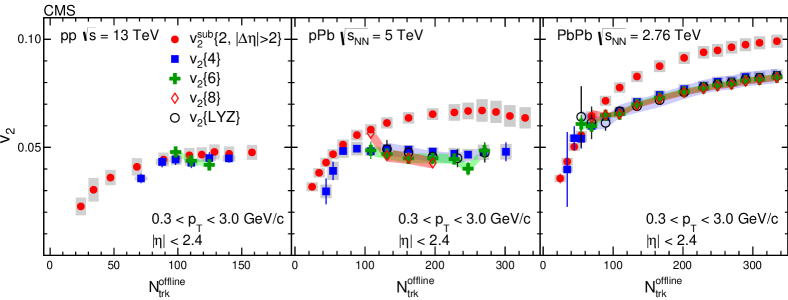
Figure 10: (colour online) Observation of multiparticle cumulants in pp, pPb and PbPb collisions. Points labelled $v_{2}\{\rm LYZ\}$ refer to the analysis method based on the Lee-Yang zeroes Bhalerao:2003yq ; Bhalerao:2003xf . The error bars correspond to the statistical uncertainties, while the shaded areas denote the systematic uncertainties. Figure from Khachatryan:2016txc .

system size and shape dependence of the functions $v_{2}(p_{T})$ and $v_{3}(p_{T})$ PHENIX:2018lia , enhanced strangeness production ALICE:2017jyt , negative $SC(3,2)$ in the highest-multiplicity pp and pPb events Sirunyan:2017uyl ; Acharya:2019vdf , etc. Azimuthal anisotropy suggests geometry-driven pressure gradients, mass ordering signifies a common velocity field of the expanding medium, ridge and multiparticle cumulants point toward a collective behaviour, strangeness enhancement indicates a deconfined medium — all leading to the proposition that perhaps “One fluid rules them all … pp, pPb, PbPb” Weller:2017tsr . However, this claim has been contested (“One fluid might not rule them all”) on the grounds that the 2+1D hydrodynamic simulations were unable to describe the multiparticle single and mixed harmonics cumulants Zhou:2020pai . Moreover, some other observables such as jet quenching, high-$p_{T}$ hadron suppression, bottomonium suppression, etc., seen in large systems have remain elusive in small-system collisions Acharya:2018qsh . So the question remains: what is the smallest size of a drop of liquid QGP? Or, can one dial the system size and switch off/on the QGP?

4.1 Origin of collectivity

Azimuthal anisotropy has long been considered as a signature of transverse collective flow Ollitrault:1992bk . It is generally agreed that the azimuthal anisotropy (for $p_{T}\lesssim 2$ GeV) in relativistic heavy-ion collisions is of hydrodynamic origin. However, at lower event multiplicities, the anisotropy can have a variety of other (nonhydrodynamic) sources (Fig. 11); for an excellent brief review see Strickland:2018exs . We shall outline only three of these competing theoretical scenarios below.

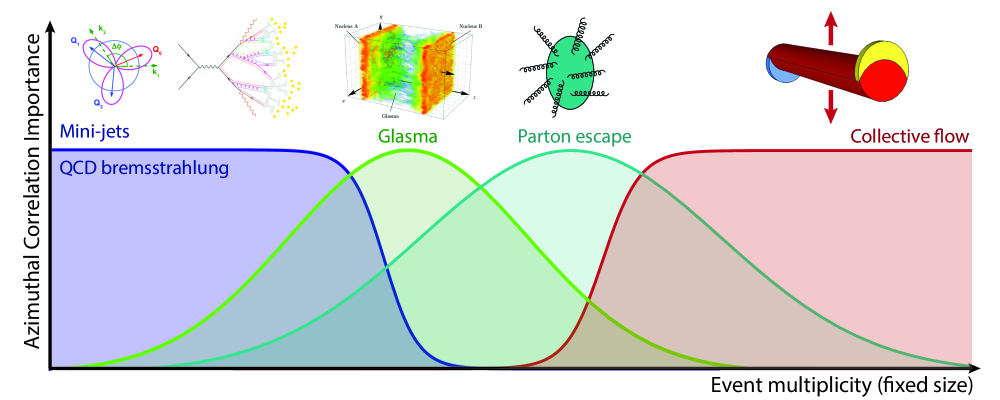
Figure 11: (colour online) A schematic diagram depicting various sources of azimuthal anisotropy as a function of event multiplicity. Vertical scale is arbitrary. Figure from Strickland:2018exs .

4.1.1 Hydrodynamics

Hydrodynamic response converts the initial spatial anisotropy of the nuclear overlap region into the momentum-space anisotropy of the final-state particles. Event-by-event relativistic second-order dissipative hydrodynamics has been successful in explaining most of the flow-related data. As an example of the success of the hydrodynamic paradigm, see Fig. 12. Note also the ordering: $v_{2}>v_{3}>v_{4}>v_{5}$. It arises because, for the 30-40% centrality results shown in Fig. 12, the shape of the initial overlap area is predominantly elliptic. The higher harmonics are driven mostly by the eccentricity fluctuations. As they probe finer details of the initial density distribution, they are successively smaller. The ordering is seen even in ideal hydrodynamic calculations; see, e.g., Gardim:2012yp . Viscous hydrodynamic calculations enhance the ordering because the higher harmonics are found to be more sensitive to the viscous attenuation. For the ultracentral collisions, the flow is driven mainly by the fluctuations rather than by the geometry, and so $v_{2}$ and $v_{3}$ are found to be similar in magnitude. Higher harmonics receive contributions from nonlinear flow modes (Sec. 3.3) and so their interpretation is not very straightforward.

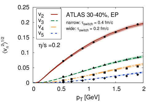
Figure 12: (colour online) Root-mean-square flow (Eq. 15) versus transverse momentum. Hydrodynamic calculations with two different switching times are compared to the ATLAS data ATLAS:2012at obtained using the event-plane (EP) method. Bands indicate statistical errors. Experimental error bars are smaller than the size of the points. Figure from Gale:2012rq .

Fluid dynamics (or loosely speaking, hydrodynamics) is an effective (macroscopic) theory that describes the slow, long-wavelength motion of a fluid close to local equilibrium. However, in the context of relativistic heavy-ion collisions, hydrodynamics is found to work very well even when the pressure in the system is far from isotropization ($p_{L}\neq p_{T}$). Secondly, applicability of hydrodynamics requires a clear separation between the microscopic and macroscopic length or time scales. Traditionally, the theory is formulated as a systematic expansion in gradients of the fluid four-velocity. Now, for small colliding systems, there is no clear separation between microscopic and macroscopic scales, or the gradients are large, and yet hydrodynamics seems to be capable of describing these systems. The above observations suggest the existence of a new theory of hydrodynamics that is applicable even far from local equilibrium Romatschke:2017vte . They have triggered a lot of theoretical activity in recent years Florkowski:2017olj .

4.1.2 Anisotropic parton-escape models

As illustrated in Fig. 11, due to the nonspherical shape of the fireball, the parton escape probability depends on the angle at which it is trying to escape, giving rise to an anisotropic momentum distribution of the detected particles, without the need of any pressure gradient. This has been demonstrated for p(d)-nucleus collisions, within the framework of transport models (e.g., AMPT) which by definition deal with dilute or low-density systems and allow only a few scatterings of partons unlike in the hydrodynamical picture He:2015hfa . Apart from the anisotropic flow, its mass ordering was also reproduced in these calculations Li:2016flp . This mechanism is expected to play an important role when the event multiplicities are somewhat lower than those corresponding to the hydrodynamic flow (Fig. 11). Interestingly, an early work that considered an expanding mixture of several species of massive relativistic particles, in the framework of the Boltzmann equation, concluded that a single collision per particle on average already leads to sizeable elliptic flow, with mass ordering between the species Borghini:2010hy . More recently, a simple kinetic theory estimate showed that for small-enough systems, even a single-hit dynamics is able to generate significant elliptic flow Kurkela:2018qeb .

4.1.3 Colour-Glass-Condensate (CGC) effective field theory

This is an effective theory of QCD at high energy. Figure 11 shows where this approach is expected to play a dominant role. Unlike hydrodynamics, this is not an initial-spatial-geometry-driven approach. Models based on this approach have intrinsic momentum-space correlations in the initial multi-gluon distribution, and hence, are called initial-state models. These correlations have a similar structure as the experimentally observed correlations. The essential physics idea is that the quarks from the small-ion projectile scatter coherently off localized domains of strong chromo-electromagnetic fields in the heavy-ion target. The colour domains are of length scale $L\sim 1/Q_{s}$, where $Q_{s}$ is the saturation scale in the target. This approach is able to reproduce many of the features of multiparticle azimuthal correlations observed in small systems Dusling:2017dqg ; Dusling:2017aot ; Mace:2018vwq . It has been argued that the large $v_{2}$ for $J/\psi$ observed at LHC can be naturally explained as the initial-state effect within the CGC formalism Zhang:2019dth ; Zhang:2020ayy . Also, the glasma initial conditions — an ensemble of approximately boost-invariant flux tubes of longitudinal colour electric and magnetic fields stretching between the colour charges in the two receding nuclei (Fig. 13) — as predicted by CGC are consistent with the long-range structure seen in the ridge phenomenon Dumitru:2010iy ; Schenke:2016lrs .

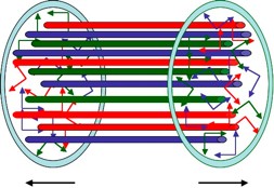
Figure 13: (colour online) Schematic representation of Glasma formed between two receding nuclei just after the collision. Figure from McLerran:2008es .

Thus the study of small systems not only deepens our understanding of (hydro)dynamics at play in large systems, but also throws light on the working of QCD in a many-body environment. Apart from Strickland:2018exs , here are some more recent reviews that cover collectivity in small systems: Ortiz:2019osu ; Morrow:2018adw ; Nagle:2018nvi ; Schenke:2017bog ; Li:2017qvf ; Schlichting:2016sqo ; Loizides:2016tew ; Dusling:2015gta .

5 Conclusions

As stated in the Introduction, this was not meant to be a comprehensive review of the phenomenology of the collective flow observed in relativistic collisions. Instead, the intention was to provide the necessary mathematical background and explain key physics concepts, in a pedagogical way, to someone uninitiated in the field, so that they can follow the literature. To that end, interspersed throughout the text are several exercises, which the reader is urged to attempt.

6 Acknowledgements

I am very thankful to Jean-Yves Ollitrault for helpful comments on the manuscript. I also thank him for our long-term collaboration which allowed me to learn many things. I acknowledge the award of the Core Research Grant, by the Science and Engineering Research Board, Department of Science and Technology, Government of India. I thank Bhavya Bhatt for drawing Fig. 14.

7 Appendix A

7.1 Moments and cumulants of a probability distribution

The $n$-th moment of a (real, continuous) function $f(x)$, about a constant $a$, is defined as

$$\mu_{n}(a)\equiv\int_{-\infty}^{\infty}(x-a)^{n}f(x)dx.$$ (A1)

We shall assume $f(x)$ to be the probability density function (PDF), normalized to unity. The two most interesting values of $a$ are 0 and $\mu\equiv\left\langle x\right\rangle$, the mean of the distribution. Usually one refers to $\mu_{n}(a=0)$ simply as the “moment” and $\mu_{n}(a=\mu)$ as the “central moment”. Henceforth, we denote moments $\mu_{n}(a=0)$ by $\mu^{\prime}_{n}$ and central moments $\mu_{n}(a=\mu)$ by $\mu_{n}$. Obviously, $\mu^{\prime}_{0}=1=\mu_{0}$ and $\mu^{\prime}_{n}=\left\langle x^{n}\right\rangle$. The first four central moments are

$$\left.\begin{aligned} \mu_{1}&=0,\\ \mu_{2}&=\left\langle x^{2}\right\rangle-\mu^{2}\equiv{\rm variance}\,(\sigma^{2})\equiv\,\,(\rm standard~{}deviation=\sigma)^{2},\\ \mu_{3}&=\left\langle x^{3}\right\rangle-3\mu\left\langle x^{2}\right\rangle+2\mu^{3},\\ \mu_{4}&=\left\langle x^{4}\right\rangle-4\mu\left\langle x^{3}\right\rangle+6\mu^{2}\left\langle x^{2}\right\rangle-3\mu^{4}.\end{aligned}\right.$$ (A2)

It is often convenient to define standardized central moments which are scale-invariant or dimensionless quantities: $\mu_{n}/\sigma^{n}$. The first four standardized central moments are

$$\left.\begin{aligned} \mu_{1}/\sigma&=0,\\ \mu_{2}/\sigma^{2}&=1,\\ \mu_{3}/\sigma^{3}&\equiv{\rm skewness}\,\,(\gamma),\\ \mu_{4}/\sigma^{4}&\equiv{\rm kurtosis}\,\,(\kappa).\end{aligned}\right.$$ (A3)

Excess kurtosis is defined as $\kappa-3$. However, it is not uncommon to find the excess kurtosis itself termed as kurtosis. The reason for subtracting 3 will become clear when we discuss the Gaussian (or normal) distribution (Appendix C).

$\bullet$ Variance is a measure of the spread of the random numbers about their mean value.

$\bullet$ Skewness is a measure of the lopsidedness or asymmetry of the distribution about its mean. It is clear from the definition that a distribution that is symmetric about its mean has vanishing skewness. In general, skewness can be positive or negative. If the left (right) tail is drawn out, or in other words, is longer than the right (left) tail, the distribution is said to be left(right)-skewed and has a negative (positive) skewness; see Fig 14.

$\bullet$ Kurtosis is a measure of the heaviness of the tails of the distribution as compared to the normal distribution with the same variance. It is clear from the definition that kurtosis is a nonnegative number. (Excess kurtosis may be positive or negative.) Kurtosis is a measure of the “tailedness” and not the “peakedness” of a distribution (Fig 14), because the proportion of the kurtosis that is determined by the central $\mu\pm\sigma$ range is usually quite small Westfall:2014phw .

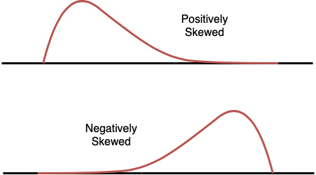
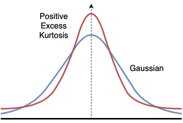
Figure 14: (colour online) (left) Positively and negatively skewed distributions. (right) Gaussian (excess kurtosis = 0, blue) and a non-Gaussian distribution with heavier tails (excess kurtosis positive, red).

7.2 Moment-generating function $M(t)$

$$M(t)\equiv\left\langle e^{tx}\right\rangle=1+t\left\langle x\right\rangle+\frac{t^{2}}{2!}\left\langle x^{2}\right\rangle+\cdots=\sum_{n=0}^{\infty}\frac{t^{n}}{n!}\left\langle x^{n}\right\rangle.$$ (A4)

Observe that the moments $\mu^{\prime}_{n}=\left\langle x^{n}\right\rangle$ appear in the above expansion. To isolate the $m$-th moment $\left\langle x^{m}\right\rangle$, for example, one uses

$$\left[\frac{d^{m}}{dt^{m}}M(t)\right]_{t=0}=\left\langle x^{m}\right\rangle.$$ (A5)

Differentiating $M(t)$   $m$ times removes the first $m$ terms, i.e., the terms containing $1,\left\langle x\right\rangle,\cdots,\left\langle x^{m-1}\right\rangle$. Further, setting $t=0$ removes terms containing $\left\langle x^{m+1}\right\rangle,\left\langle x^{m+2}\right\rangle,$ $\cdots$, leaving behind only $\left\langle x^{m}\right\rangle$. The moment-generating function provides an alternative description of the PDF. The central moment generating function is $e^{-\mu t}M(t)$.

7.3 Cumulant-generating function $K(t)$

$$K(t)\equiv\ln M(t)=\ln\left\langle e^{tx}\right\rangle=t\kappa_{1}+\frac{t^{2}}{2!}\kappa_{2}+\frac{t^{3}}{3!}\kappa_{3}+\cdots=\sum_{n=1}^{\infty}\frac{t^{n}}{n!}\kappa_{n},$$ (A6)

where $\kappa_{n}$ are the cumulants. To isolate the $m$-th cumulant $\kappa_{m}$, for example, one uses

$$\left[\frac{d^{m}}{dt^{m}}K(t)\right]_{t=0}=\kappa_{m}.$$ (A7)

Differentiating $K(t)$   $m$ times removes the first $m-1$ terms, i.e., the terms containing $\kappa_{1},\cdots,\kappa_{m-1}$. Further, setting $t=0$ removes terms containing $\kappa_{m+1},\kappa_{m+2},\cdots$, leaving behind only $\kappa_{m}$. It is straightforward to show that the first few cumulants are

$$\left.\begin{aligned} \kappa_{1}&=\left\langle x\right\rangle={\rm mean}\,\,\mu,\\ \kappa_{2}&=\left\langle x^{2}\right\rangle-\left\langle x\right\rangle^{2}=\left\langle(x-\left\langle x\right\rangle)^{2}\right\rangle={\rm variance}\,\,(\sigma^{2})={\rm second\,\,central\,\,moment},\\ \kappa_{3}&=\left\langle x^{3}\right\rangle-3\left\langle x\right\rangle\left\langle x^{2}\right\rangle+2\left\langle x\right\rangle^{3}=\left\langle(x-\left\langle x\right\rangle)^{3}\right\rangle={\rm third\,\,central\,\,moment},\\ \kappa_{4}&=\left\langle x^{4}\right\rangle-4\left\langle x\right\rangle\left\langle x^{3}\right\rangle-3\left\langle x^{2}\right\rangle^{2}+12\left\langle x\right\rangle^{2}\left\langle x^{2}\right\rangle-6\left\langle x\right\rangle^{4}\\ &\neq{\rm fourth\,\,central\,\,moment}\,\,\left\langle(x-\left\langle x\right\rangle)^{4}\right\rangle,\\ \kappa_{5}&=\left\langle x^{5}\right\rangle-5\left\langle x\right\rangle\left\langle x^{4}\right\rangle-10\left\langle x^{2}\right\rangle\left\langle x^{3}\right\rangle+20\left\langle x\right\rangle^{2}\left\langle x^{3}\right\rangle+30\left\langle x\right\rangle\left\langle x^{2}\right\rangle^{2}\\ &-60\left\langle x\right\rangle^{3}\left\langle x^{2}\right\rangle+24\left\langle x\right\rangle^{5},\\ \kappa_{6}&=\left\langle x^{6}\right\rangle-6\left\langle x\right\rangle\left\langle x^{5}\right\rangle-15\left\langle x^{2}\right\rangle\left\langle x^{4}\right\rangle+30\left\langle x\right\rangle^{2}\left\langle x^{4}\right\rangle-10\left\langle x^{3}\right\rangle^{2}+120\left\langle x\right\rangle\left\langle x^{2}\right\rangle\left\langle x^{3}\right\rangle\\ &-120\left\langle x\right\rangle^{3}\left\langle x^{3}\right\rangle+30\left\langle x^{2}\right\rangle^{3}-270\left\langle x\right\rangle^{2}\left\langle x^{2}\right\rangle^{2}+360\left\langle x\right\rangle^{4}\left\langle x^{2}\right\rangle-120\left\langle x\right\rangle^{6}.\end{aligned}\right.$$ (A8)

Fourth- and higher-order cumulants are not identical to the corresponding central moments. Thus cumulants are certain polynomial functions of the moments and provide an alternative to the moments of the distribution.

The above equations can be inverted to express moments in terms of cumulants:

$$\left.\begin{aligned} \left\langle x\right\rangle&=\kappa_{1},\\ \left\langle x^{2}\right\rangle&=\kappa_{1}^{2}+\kappa_{2},\\ \left\langle x^{3}\right\rangle&=\kappa_{1}^{3}+3\kappa_{1}\kappa_{2}+\kappa_{3},\\ \left\langle x^{4}\right\rangle&=\kappa_{1}^{4}+6\kappa_{1}^{2}\kappa_{2}+4\kappa_{1}\kappa_{3}+3\kappa_{2}^{2}+\kappa_{4},\\ \left\langle x^{5}\right\rangle&=\kappa_{1}^{5}+10\kappa_{1}^{3}\kappa_{2}+10\kappa_{1}^{2}\kappa_{3}+15\kappa_{1}\kappa_{2}^{2}+5\kappa_{1}\kappa_{4}+10\kappa_{2}\kappa_{3}+\kappa_{5},\\ \left\langle x^{6}\right\rangle&=\kappa_{1}^{6}+6\kappa_{1}\kappa_{5}+15\kappa_{1}^{2}\kappa_{4}+20\kappa_{1}^{3}\kappa_{3}+15\kappa_{1}^{4}\kappa_{2}+60\kappa_{1}\kappa_{2}\kappa_{3}+45\kappa_{1}^{2}\kappa_{2}^{2}+15\kappa_{2}\kappa_{4}\\ &+10\kappa_{3}^{2}+15\kappa_{2}^{3}+\kappa_{6}.\end{aligned}\right.$$ (A9)

8 Appendix B

8.1 Correlation functions and cumulants

The $n$-particle correlation function (or simply a correlator) $\rho(1,2,3,\cdots,n)$ consists of terms that represent combinations of lower-order correlations and a term that represents a genuine or “true” $n$-particle correlation $C(1,2,3,\cdots,n)$ which is called a cumulant. For example, $\rho(1,2)=\rho(1)\rho(2)+C(1,2)$, so that $C(1,2)=\rho(1,2)-\rho(1)\rho(2)$. If the two particles are statistically independent, $\rho(1,2)$ simply reduces to $\rho(1)\rho(2)$, whereas $C(1,2)$ vanishes by construction. The first few correlation functions are Bzdak:2015dja

$$\left.\begin{aligned} \rho(1)&=C(1),\\ \rho(1,2)&=\rho(1)\rho(2)+C(1,2),\\ \rho(1,2,3)&=\rho(1)\rho(2)\rho(3)+\rho(1)C(2,3)+\rho(2)C(3,1)+\rho(3)C(1,2)+C(1,2,3),\\ &\equiv\rho(1)\rho(2)\rho(3)+\sum_{(3)}\rho(1)C(2,3)+C(1,2,3),\\ \rho(1,2,3,4)&=\rho(1)\rho(2)\rho(3)\rho(4)+\sum_{(6)}\rho(1)\rho(2)C(3,4)+\sum_{(4)}\rho(1)C(2,3,4)\\ &+\sum_{(3)}C(1,2)C(3,4)+C(1,2,3,4),\\ \rho(1,2,3,4,5)&=\rho(1)\rho(2)\rho(3)\rho(4)\rho(5)+\sum_{(10)}\rho(1)\rho(2)\rho(3)C(4,5)\\ &+\sum_{(10)}\rho(1)\rho(2)C(3,4,5)+\sum_{(15)}\rho(1)C(2,3)C(4,5)\\ &+\sum_{(5)}\rho(1)C(2,3,4,5)+\sum_{(10)}C(1,2)C(3,4,5)+C(1,2,3,4,5),\\ \rho(1,2,3,4,5,6)&=\rho(1)\rho(2)\rho(3)\rho(4)\rho(5)\rho(6)+\sum_{(6)}\rho(1)C(2,3,4,5,6)\\ &+\sum_{(15)}\rho(1)\rho(2)C(3,4,5,6)+\sum_{(20)}\rho(1)\rho(2)\rho(3)C(4,5,6)\\ &+\sum_{(15)}\rho(1)\rho(2)\rho(3)\rho(4)C(5,6)+\sum_{(60)}\rho(1)C(2,3)C(4,5,6)\\ &+\sum_{(45)}\rho(1)\rho(2)C(3,4)C(5,6)+\sum_{(15)}C(1,2)C(3,4,5,6)\\ &+\sum_{(10)}C(1,2,3)C(4,5,6)+\sum_{(15)}C(1,2)C(3,4)C(5,6)\\ &+C(1,2,3,4,5,6),\end{aligned}\right.$$ (B1)

where the numbers in parentheses under the summation signs indicate the number of possible permutations of the indices.

The above equations can be inverted to get the expressions for the cumulants in terms of the correlation functions:

$$\left.\begin{aligned} C(1)&=\rho(1),\\ C(1,2)&=\rho(1,2)-\rho(1)\rho(2),\\ C(1,2,3)&=\rho(1,2,3)-\sum_{(3)}\rho(1)\rho(2,3)+2\rho(1)\rho(2)\rho(3),\\ C(1,2,3,4)&=\rho(1,2,3,4)-\sum_{(4)}\rho(1)\rho(2,3,4)-\sum_{(3)}\rho(1,2)\rho(3,4)\\ &+2\sum_{(6)}\rho(1)\rho(2)\rho(3,4)-6\rho(1)\rho(2)\rho(3)\rho(4),\\ C(1,2,3,4,5)&=\rho(1,2,3,4,5)-\sum_{(5)}\rho(1)\rho(2,3,4,5)-\sum_{(10)}\rho(1,2)\rho(3,4,5)\\ &+2\sum_{(10)}\rho(1)\rho(2)\rho(3,4,5)+2\sum_{(15)}\rho(1)\rho(2,3)\rho(4,5)\\ &-6\sum_{(10)}\rho(1)\rho(2)\rho(3)\rho(4,5)+24\rho(1)\rho(2)\rho(3)\rho(4)\rho(5),\\ C(1,2,3,4,5,6)&=\rho(1,2,3,4,5,6)-\sum_{(6)}\rho(1)\rho(2,3,4,5,6)-\sum_{(15)}\rho(1,2)\rho(3,4,5,6)\\ &+2\sum_{(15)}\rho(1)\rho(2)\rho(3,4,5,6)-\sum_{(10)}\rho(1,2,3)\rho(4,5,6)\\ &+4\sum_{(30)}\rho(1)\rho(2,3)\rho(4,5,6)-6\sum_{(20)}\rho(1)\rho(2)\rho(3)\rho(4,5,6)\\ &+2\sum_{(15)}\rho(1,2)\rho(3,4)\rho(5,6)-3\sum_{(90)}\rho(1)\rho(2)\rho(3,4)\rho(5,6)\\ &+24\sum_{(15)}\rho(1)\rho(2)\rho(3)\rho(4)\rho(5,6)-\sum_{(120)}\rho(1)\rho(2)\rho(3)\rho(4)\rho(5)\rho(6).\end{aligned}\right.$$ (B2)

It is easy to verify that the cumulant vanishes if any one or more particles is statistically independent of the others. Thus the $n$-particle cumulant measures the statistical dependence of the entire $n$-particle set. For this reason, cumulants are also called connected correlation functions.

Exercise 11: Compare the above expressions of cumulants to those in Appendix A.

Exercise 12: Note how the above expressions of correlators and cumulants simplify considerably if the single-particle $\rho$ vanishes.

9 Appendix C

9.1 Gaussian or normal distribution in 1D

One-dimensional Gaussian (centered at $\mu$) is

$$f(x)=\frac{1}{\sigma\sqrt{2\pi}}\exp\left[-\frac{(x-\mu)^{2}}{2\sigma^{2}}\right],$$ (C1)

where $\mu=\left\langle x\right\rangle$ is the mean, $\sigma^{2}$ is the variance and $f(x)$ is normalized to unity. The odd central moments are obviously zero. The even central moments are given by $(n-1)!!\,\sigma^{n}\,\,(n~{}{\rm even})$. The first few even central moments are given in Table 1. The skewness ($\gamma$) is zero, kurtosis ($\kappa$) is 3 and excess kurtosis ($\kappa-3$) is zero. A probability distribution with tails heavier (lighter) than those of the normal distribution shows a higher (lower) propensity to produce outliers and has a positive (negative) excess kurtosis (Fig 14),

Table 1: First few central and noncentral moments of the Gaussian distribution

Order	Central moment	Noncentral moment
1	0	$\mu$
2	$\sigma^{2}$	$\mu^{2}+\sigma^{2}$
3	0	$\mu^{3}+3\mu\sigma^{2}$
4	$3\,\sigma^{4}$	$\mu^{4}+6\mu^{2}\sigma^{2}+3\sigma^{4}$
5	0	$\mu^{5}+10\mu^{3}\sigma^{2}+15\mu\sigma^{4}$
6	$15\,\sigma^{6}$	$\mu^{6}+15\mu^{4}\sigma^{2}+45\mu^{2}\sigma^{4}+15\sigma^{6}$
7	0	$\mu^{7}+21\mu^{5}\sigma^{2}+105\mu^{3}\sigma^{4}+105\mu\sigma^{6}$
8	$105\,\sigma^{8}$	$\mu^{8}+28\mu^{6}\sigma^{2}+210\mu^{4}\sigma^{4}+420\mu^{2}\sigma^{6}+105\sigma^{8}$

For the normal distribution, the moment-generating function is $M(t)=\exp\,(\mu t+(\sigma^{2}t^{2}/2))$ and the cumulant-generating function is $K(t)=\ln M(t)=\mu t+(\sigma^{2}t^{2}/2)$. Since this is a quadratic in $t$, only the first two cumulants survive, namely the mean $\mu$ and the variance $\sigma^{2}$. It can be shown that the normal distribution is the only one for which the third and higher cumulants vanish.

Exercise 13: Using the expressions for moments in terms of cumulants given in Appendix A, show that the first six noncentral moments of the normal distribution are as given in Table 1.

9.2 Gaussian or normal distribution in 2D

Two-dimensional Gaussian centered at the origin and normalized to unity is

$$f(x,y)=\frac{1}{2\pi\sigma_{x}\sigma_{y}}\exp\left[-\frac{x^{2}}{2\sigma_{x}^{2}}-\frac{y^{2}}{2\sigma_{y}^{2}}\right],$$ (C2)

where $\sigma_{x}^{2}$ and $\sigma_{y}^{2}$ are the variances.

Exercise 14: For an asymmetric ($\sigma_{x}\neq\sigma_{y}$) 2D Gaussian as in Eq. (C2), let $z=x+iy$. Show that the fourth moment $\langle z^{4}\rangle\neq 0$, and is trivially correlated with the second moment $\langle z^{2}\rangle$. However, the fourth-order cumulant $\langle z^{4}\rangle-3\langle z^{2}\rangle^{2}=0$.

It is often convenient to introduce the symmetric case ($\sigma_{x}=\sigma_{y}$) and write it in terms of $r=\sqrt{x^{2}+y^{2}}$:

$$f(r)=\frac{1}{\pi\sigma^{2}}\exp\left[-\frac{r^{2}}{\sigma^{2}}\right],$$ (C3)

where $\sigma^{2}\equiv\sigma_{x}^{2}+\sigma_{y}^{2}$. $f(r)$ is also centered at the origin and normalized to unity. Note, however, that unlike $\left\langle x\right\rangle$ and $\left\langle y\right\rangle$, $\left\langle r\right\rangle$ is not zero. The first few moments of $f(r)$, $\mu_{n}=\left\langle r^{n}\right\rangle=\sigma^{n}\,\Gamma((n/2)+1)$, are given in Table 2. Note also that $\left\langle r^{2}\right\rangle=\left\langle x^{2}\right\rangle+\left\langle y^{2}\right\rangle$; using $\left\langle r^{2}\right\rangle$ from Table 2, we get $\sigma^{2}=\sigma_{x}^{2}+\sigma_{y}^{2}$. The kurtosis in this case is 2, unlike the case of a 1D Gaussian discussed earlier where it was 3.

Table 2: First few moments ($\mu_{n}$) of $f(r)$, Eq. (C3)

$n$	1	2	3	4	5	6	7	8
$\mu_{n}$	$\sqrt{\pi}\,\sigma/2$	$\sigma^{2}$	$3\sqrt{\pi}\,\sigma^{3}/4$	$2\,\sigma^{4}$	$15\sqrt{\pi}\,\sigma^{5}/8$	$6\,\sigma^{6}$	$105\sqrt{\pi}\,\sigma^{7}/16$	$24\,\sigma^{8}$

References

- (1) S. A. Chin, Phys. Lett. 78B (1978) 552 doi:10.1016/0370-2693(78)90637-8
- (2) F. B. Yano and S. E. Koonin, Phys. Lett. 78B (1978) 556 doi:10.1016/0370-2693(78)90638-X
- (3) S. A. Voloshin, A. M. Poskanzer and R. Snellings, Landolt-Bornstein 23 (2010) 293 [arXiv:0809.2949 [nucl-ex]].
- (4) B. Alver and G. Roland, Phys. Rev. C 81 (2010) 054905, Erratum: [Phys. Rev. C 82 (2010) 039903] doi:10.1103/PhysRevC.82.039903, 10.1103/PhysRevC.81.054905 [arXiv:1003.0194 [nucl-th]].
- (5) U. Heinz and R. Snellings, Ann. Rev. Nucl. Part. Sci. 63 (2013), 123-151 doi:10.1146/annurev-nucl-102212-170540 [arXiv:1301.2826 [nucl-th]].
- (6) D. Teaney and L. Yan, Phys. Rev. C 90, no. 2 (2014) 024902 doi:10.1103/PhysRevC.90.024902 [arXiv:1312.3689 [nucl-th]].
- (7) J. Y. Ollitrault, Phys. Rev. D 46 (1992) 229. doi:10.1103/PhysRevD.46.229
- (8) S. Voloshin and Y. Zhang, Z. Phys. C 70 (1996) 665 doi:10.1007/s002880050141 [hep-ph/9407282].
- (9) M. Luzum, J. Phys. G 38 (2011) 124026 doi:10.1088/0954-3899/38/12/124026 [arXiv:1107.0592 [nucl-th]].
- (10) A. M. Poskanzer and S. A. Voloshin, Phys. Rev. C 58 (1998) 1671 doi:10.1103/PhysRevC.58.1671 [nucl-ex/9805001].
- (11) J. Y. Ollitrault, nucl-ex/9711003.
- (12) S. Acharya et al. [ALICE Collaboration], arXiv:2002.00633 [nucl-ex].
- (13) V. Khachatryan et al. [CMS Collaboration], Phys. Rev. C 92 (2015) no.3, 034911 doi:10.1103/PhysRevC.92.034911 [arXiv:1503.01692 [nucl-ex]].
- (14) P. Bozek, W. Broniowski and J. Moreira, Phys. Rev. C 83 (2011) 034911 doi:10.1103/PhysRevC.83.034911 [arXiv:1011.3354 [nucl-th]].
- (15) N. Borghini, P. M. Dinh and J. Y. Ollitrault, Phys. Rev. C 64 (2001) 054901 doi:10.1103/PhysRevC.64.054901 [nucl-th/0105040].
- (16) R. S. Bhalerao and J. Y. Ollitrault, Phys. Lett. B 641 (2006) 260 doi:10.1016/j.physletb.2006.08.055 [nucl-th/0607009].
- (17) P. Di Francesco, M. Guilbaud, M. Luzum and J. Y. Ollitrault, Phys. Rev. C 95 (2017) no.4, 044911 doi:10.1103/PhysRevC.95.044911 [arXiv:1612.05634 [nucl-th]].
- (18) Z. Moravcova, K. Gulbrandsen and Y. Zhou, [arXiv:2005.07974 [nucl-th]].
- (19) G. Aad et al. [ATLAS Collaboration], JHEP 1311 (2013) 183 doi:10.1007/JHEP11(2013)183 [arXiv:1305.2942 [hep-ex]].
- (20) S. Acharya et al. [ALICE Collaboration], JHEP 1807 (2018) 103 doi:10.1007/JHEP07(2018)103 [arXiv:1804.02944 [nucl-ex]].
- (21) J. Y. Ollitrault, A. M. Poskanzer and S. A. Voloshin, Phys. Rev. C 80 (2009) 014904 doi:10.1103/PhysRevC.80.014904 [arXiv:0904.2315 [nucl-ex]].
- (22) A. M. Sirunyan et al. [CMS Collaboration], Phys. Lett. B 789 (2019) 643 doi:10.1016/j.physletb.2018.11.063 [arXiv:1711.05594 [nucl-ex]].
- (23) S. A. Voloshin, A. M. Poskanzer, A. Tang and G. Wang, Phys. Lett. B 659 (2008) 537 doi:10.1016/j.physletb.2007.11.043 [arXiv:0708.0800 [nucl-th]].
- (24) M. Aaboud et al. [ATLAS], JHEP 01 (2020), 051 doi:10.1007/JHEP01(2020)051 [arXiv:1904.04808 [nucl-ex]].
- (25) L. Yan, J. Y. Ollitrault and A. M. Poskanzer, Phys. Rev. C 90 (2014) no.2, 024903 doi:10.1103/PhysRevC.90.024903 [arXiv:1405.6595 [nucl-th]].
- (26) G. Giacalone, L. Yan, J. Noronha-Hostler and J. Y. Ollitrault, Phys. Rev. C 95 (2017) no.1, 014913 doi:10.1103/PhysRevC.95.014913 [arXiv:1608.01823 [nucl-th]].
- (27) R. S. Bhalerao, G. Giacalone and J. Y. Ollitrault, Phys. Rev. C 99 (2019) no.1, 014907 doi:10.1103/PhysRevC.99.014907 [arXiv:1811.00837 [nucl-th]].
- (28) R. S. Bhalerao, G. Giacalone and J. Y. Ollitrault, Phys. Rev. C 100 (2019) no.1, 014909 doi:10.1103/PhysRevC.100.014909 [arXiv:1904.10350 [nucl-th]].
- (29) S. Chatrchyan et al. [CMS Collaboration], Phys. Lett. B 724 (2013) 213 doi:10.1016/j.physletb.2013.06.028 [arXiv:1305.0609 [nucl-ex]].
- (30) V. Khachatryan et al. [CMS Collaboration], Phys. Lett. B 765 (2017) 193 doi:10.1016/j.physletb.2016.12.009 [arXiv:1606.06198 [nucl-ex]].
- (31) S. Chatrchyan et al. [CMS Collaboration], JHEP 1402 (2014) 088 doi:10.1007/JHEP02(2014)088 [arXiv:1312.1845 [nucl-ex]].
- (32) A. Dumitru, F. Gelis, L. McLerran and R. Venugopalan, Nucl. Phys. A 810 (2008) 91 doi:10.1016/j.nuclphysa.2008.06.012 [arXiv:0804.3858 [hep-ph]].
- (33) F. G. Gardim, F. Grassi, M. Luzum and J. Y. Ollitrault, Phys. Rev. C 87 (2013) no.3, 031901 doi:10.1103/PhysRevC.87.031901 [arXiv:1211.0989 [nucl-th]].
- (34) M. Aaboud et al. [ATLAS Collaboration], Eur. Phys. J. C 78 (2018) no.2, 142 doi:10.1140/epjc/s10052-018-5605-7 [arXiv:1709.02301 [nucl-ex]].
- (35) G. Aad et al. [ATLAS Collaboration], arXiv:2001.04201 [nucl-ex].
- (36) R. S. Bhalerao, M. Luzum and J. Y. Ollitrault, Phys. Rev. C 84 (2011), 034910 doi:10.1103/PhysRevC.84.034910 [arXiv:1104.4740 [nucl-th]].
- (37) R. S. Bhalerao, M. Luzum and J. Y. Ollitrault, J. Phys. G 38 (2011), 124055 doi:10.1088/0954-3899/38/12/124055 [arXiv:1106.4940 [nucl-ex]].
- (38) J. Adam et al. [ALICE Collaboration], Phys. Rev. Lett. 117 (2016) 182301 doi:10.1103/PhysRevLett.117.182301 [arXiv:1604.07663 [nucl-ex]].
- (39) S. Acharya et al. [ALICE Collaboration], Phys. Rev. C 97 (2018) no.2, 024906 doi:10.1103/PhysRevC.97.024906 [arXiv:1709.01127 [nucl-ex]].
- (40) A. M. Sirunyan et al. [CMS], Phys. Rev. Lett. 120 (2018) no.9, 092301 doi:10.1103/PhysRevLett.120.092301 [arXiv:1709.09189 [nucl-ex]].
- (41) S. Acharya et al. [ALICE], Phys. Rev. Lett. 123 (2019) no.14, 142301 doi:10.1103/PhysRevLett.123.142301 [arXiv:1903.01790 [nucl-ex]].
- (42) C. Mordasini, A. Bilandzic, D. Karakoç and S. F. Taghavi, Phys. Rev. C 102 (2020) no.2, 024907 doi:10.1103/PhysRevC.102.024907 [arXiv:1901.06968 [nucl-ex]].
- (43) R. S. Bhalerao, J. Y. Ollitrault and S. Pal, Phys. Rev. C 88 (2013) 024909 doi:10.1103/PhysRevC.88.024909 [arXiv:1307.0980 [nucl-th]].
- (44) G. Aad et al. [ATLAS Collaboration], Phys. Rev. C 90 (2014) no.2, 024905 doi:10.1103/PhysRevC.90.024905 [arXiv:1403.0489 [hep-ex]].
- (45) S. Acharya et al. [ALICE Collaboration], Phys. Lett. B 773 (2017) 68 doi:10.1016/j.physletb.2017.07.060 [arXiv:1705.04377 [nucl-ex]].
- (46) A. Bilandzic, M. Lesch and S. F. Taghavi, Phys. Rev. C 102 (2020) no.2, 024910 doi:10.1103/PhysRevC.102.024910 [arXiv:2004.01066 [nucl-ex]].
- (47) D. Teaney and L. Yan, Phys. Rev. C 86 (2012), 044908 doi:10.1103/PhysRevC.86.044908 [arXiv:1206.1905 [nucl-th]].
- (48) J. Qian, U. W. Heinz and J. Liu, Phys. Rev. C 93 (2016) no.6, 064901 doi:10.1103/PhysRevC.93.064901 [arXiv:1602.02813 [nucl-th]].
- (49) R. S. Bhalerao, J. Y. Ollitrault and S. Pal, Phys. Lett. B 742 (2015), 94-98 doi:10.1016/j.physletb.2015.01.019 [arXiv:1411.5160 [nucl-th]].
- (50) L. Yan and J. Y. Ollitrault, Phys. Lett. B 744 (2015), 82-87 doi:10.1016/j.physletb.2015.03.040 [arXiv:1502.02502 [nucl-th]].
- (51) J. Qian, U. Heinz, R. He and L. Huo, Phys. Rev. C 95 (2017) no.5, 054908 doi:10.1103/PhysRevC.95.054908 [arXiv:1703.04077 [nucl-th]].
- (52) G. Aad et al. [ATLAS], Phys. Rev. C 92 (2015) no.3, 034903 doi:10.1103/PhysRevC.92.034903 [arXiv:1504.01289 [hep-ex]].
- (53) M. Aaboud et al. [ATLAS Collaboration], Phys. Rev. C 96 (2017) no.2, 024908 doi:10.1103/PhysRevC.96.024908 [arXiv:1609.06213 [nucl-ex]].
- (54) V. Pacík [ALICE Collaboration], Nucl. Phys. A 982 (2019) 451 doi:10.1016/j.nuclphysa.2018.09.020 [arXiv:1807.04538 [nucl-ex]].
- (55) R. S. Bhalerao, N. Borghini and J. Y. Ollitrault, Phys. Lett. B 580 (2004), 157-162 doi:10.1016/j.physletb.2003.11.056 [arXiv:nucl-th/0307018 [nucl-th]].
- (56) R. S. Bhalerao, N. Borghini and J. Y. Ollitrault, Nucl. Phys. A 727 (2003), 373-426 doi:10.1016/j.nuclphysa.2003.08.007 [arXiv:nucl-th/0310016 [nucl-th]].
- (57) C. Aidala et al. [PHENIX Collaboration], Nature Phys. 15 (2019) no.3, 214 doi:10.1038/s41567-018-0360-0 [arXiv:1805.02973 [nucl-ex]].
- (58) J. Adam et al. [ALICE Collaboration], Nature Phys. 13 (2017) 535 doi:10.1038/nphys4111 [arXiv:1606.07424 [nucl-ex]].
- (59) R. D. Weller and P. Romatschke, Phys. Lett. B 774 (2017) 351 doi:10.1016/j.physletb.2017.09.077 [arXiv:1701.07145 [nucl-th]].
- (60) Y. Zhou, W. Zhao, K. Murase and H. Song, [arXiv:2005.02684 [nucl-th]].
- (61) S. Acharya et al. [ALICE Collaboration], JHEP 1811 (2018) 013 doi:10.1007/JHEP11(2018)013 [arXiv:1802.09145 [nucl-ex]].
- (62) M. Strickland, Nucl. Phys. A 982 (2019) 92 doi:10.1016/j.nuclphysa.2018.09.071 [arXiv:1807.07191 [nucl-th]].
- (63) G. Aad et al. [ATLAS Collaboration], Phys. Rev. C 86 (2012) 014907 doi:10.1103/PhysRevC.86.014907 [arXiv:1203.3087 [hep-ex]].
- (64) C. Gale, S. Jeon, B. Schenke, P. Tribedy and R. Venugopalan, Phys. Rev. Lett. 110 (2013) no.1, 012302 doi:10.1103/PhysRevLett.110.012302 [arXiv:1209.6330 [nucl-th]].
- (65) F. G. Gardim, F. Grassi, M. Luzum and J. Y. Ollitrault, Phys. Rev. Lett. 109 (2012) 202302 doi:10.1103/PhysRevLett.109.202302 [arXiv:1203.2882 [nucl-th]].
- (66) P. Romatschke, Phys. Rev. Lett. 120 (2018) no.1, 012301 doi:10.1103/PhysRevLett.120.012301 [arXiv:1704.08699 [hep-th]].
- (67) W. Florkowski, M. P. Heller and M. Spalinski, Rept. Prog. Phys. 81 (2018) no.4, 046001 doi:10.1088/1361-6633/aaa091 [arXiv:1707.02282 [hep-ph]].
- (68) L. He, T. Edmonds, Z. W. Lin, F. Liu, D. Molnar and F. Wang, Phys. Lett. B 753 (2016) 506 doi:10.1016/j.physletb.2015.12.051 [arXiv:1502.05572 [nucl-th]].
- (69) H. Li, L. He, Z. W. Lin, D. Molnar, F. Wang and W. Xie, Phys. Rev. C 93 (2016) no.5, 051901 doi:10.1103/PhysRevC.93.051901 [arXiv:1601.05390 [nucl-th]].
- (70) N. Borghini and C. Gombeaud, Eur. Phys. J. C 71 (2011), 1612 doi:10.1140/epjc/s10052-011-1612-7 [arXiv:1012.0899 [nucl-th]].
- (71) A. Kurkela, U. A. Wiedemann and B. Wu, Eur. Phys. J. C 79 (2019) no.9, 759 doi:10.1140/epjc/s10052-019-7262-x [arXiv:1805.04081 [hep-ph]].
- (72) K. Dusling, M. Mace and R. Venugopalan, Phys. Rev. Lett. 120 (2018) no.4, 042002 doi:10.1103/PhysRevLett.120.042002 [arXiv:1705.00745 [hep-ph]].
- (73) K. Dusling, M. Mace and R. Venugopalan, Phys. Rev. D 97 (2018) no.1, 016014 doi:10.1103/PhysRevD.97.016014 [arXiv:1706.06260 [hep-ph]].
- (74) M. Mace, V. V. Skokov, P. Tribedy and R. Venugopalan, Phys. Rev. Lett. 121 (2018) no.5, 052301 Erratum: [Phys. Rev. Lett. 123 (2019) no.3, 039901] doi:10.1103/PhysRevLett.123.039901, 10.1103/PhysRevLett.121.052301 [arXiv:1805.09342 [hep-ph]].
- (75) C. Zhang, C. Marquet, G. Y. Qin, S. Y. Wei and B. W. Xiao, Phys. Rev. Lett. 122 (2019) no.17, 172302 doi:10.1103/PhysRevLett.122.172302 [arXiv:1901.10320 [hep-ph]].
- (76) C. Zhang, C. Marquet, G. Y. Qin, Y. Shi, L. Wang, S. Y. Wei and B. W. Xiao, arXiv:2002.09878 [hep-ph].
- (77) L. McLerran, doi:10.3204/DESY-PROC-2009-01/26 arXiv:0812.4989 [hep-ph].
- (78) A. Dumitru, K. Dusling, F. Gelis, J. Jalilian-Marian, T. Lappi and R. Venugopalan, Phys. Lett. B 697 (2011) 21 doi:10.1016/j.physletb.2011.01.024 [arXiv:1009.5295 [hep-ph]].
- (79) B. Schenke, S. Schlichting, P. Tribedy and R. Venugopalan, Phys. Rev. Lett. 117 (2016) no.16, 162301 doi:10.1103/PhysRevLett.117.162301 [arXiv:1607.02496 [hep-ph]].
- (80) A. Ortiz [ALICE and ATLAS and CMS and LHCb Collaborations], PoS LHCP 2019 (2019) 091 doi:10.22323/1.350.0091 [arXiv:1909.03937 [hep-ex]].
- (81) S. Morrow [PHENIX Collaboration], arXiv:1810.05321 [nucl-ex].
- (82) J. L. Nagle and W. A. Zajc, Ann. Rev. Nucl. Part. Sci. 68 (2018) 211 doi:10.1146/annurev-nucl-101916-123209 [arXiv:1801.03477 [nucl-ex]].
- (83) B. Schenke, Nucl. Phys. A 967 (2017) 105 doi:10.1016/j.nuclphysa.2017.05.017 [arXiv:1704.03914 [nucl-th]].
- (84) W. Li, Nucl. Phys. A 967 (2017) 59 doi:10.1016/j.nuclphysa.2017.05.011 [arXiv:1704.03576 [nucl-ex]].
- (85) S. Schlichting and P. Tribedy, Adv. High Energy Phys. 2016 (2016) 8460349 doi:10.1155/2016/8460349 [arXiv:1611.00329 [hep-ph]].
- (86) C. Loizides, Nucl. Phys. A 956 (2016) 200 doi:10.1016/j.nuclphysa.2016.04.022 [arXiv:1602.09138 [nucl-ex]].
- (87) K. Dusling, W. Li and B. Schenke, Int. J. Mod. Phys. E 25 (2016) no.01, 1630002 doi:10.1142/S0218301316300022 [arXiv:1509.07939 [nucl-ex]].
- (88) P. H Westfall, The American Statistician 68, no. 3 (2014) 191 doi: 10.1080/00031305.2014.917055.
- (89) A. Bzdak and P. Bozek, Phys. Rev. C 93, no. 2 (2016) 024903 doi:10.1103/PhysRevC.93.024903 [arXiv:1509.02967 [hep-ph]].