Phase Competition in HfO₂ with Applied Electric Field from First Principles

Abstract

In this work, the results of first-principles density–functional–theory calculations are used to construct the energy landscapes of HfO₂ and its Y and Zr substituted derivatives as a function of symmetry–adapted lattice-mode amplitudes. These complex energy landscapes possess multiple local minima, corresponding to the tetragonal, oIII ($Pca2_{1}$), and oIV ($Pmn2_{1}$) phases. We find that the energy barrier between the non–polar tetragonal phase and the ferroelectric oIII phase can be lowered by Y and Zr substitution. In Hf_0.5Zr_0.5O₂ with an ordered cation arrangement, Zr substitution makes the oIV phase unstable, and it become an intermediate state in the tetragonal to oIII phase transition. Using these energy landscapes, we interpret the structural transformations and hysteresis loops computed for electric-field cycles with various choices of field direction. The implications of these results for interpreting experimental observations, such as the wake–up and split–up effects, are also discussed. These results and analysis deepen our understanding of the origin of ferroelectricity and field cycling behaviors in HfO₂–based films, and allow us to propose strategies for improving their functional properties.

I Introduction

Hafnia (HfO₂) has long been recognized as a high–$\kappa$ material, valuable in complementary metal–oxide–semiconductor (CMOS) applications Bohr et al. (2007); Gutowski et al. (2002). In 2011, Si–doped HfO₂ thin films under mechanically encapsulated crystallization were observed to be ferroelectric Böscke et al. (2011a), which led to a renewal of scientific interest and much recent theoretical and experimental research Böscke et al. (2011a, b); Mueller et al. (2012a, b); Müller et al. (2011a, b); Müller et al. (2012).

HfO₂ is a binary oxide with a number of polymorphs. At high temperatures ($T>2773$ K), bulk HfO₂ has a high–symmetry $Fm\overline{3}m$ cubic fluorite structure, in which each Hf atom is located at the center of an oxygen cube [Fig.1 (a)]. As the temperature decreases (2773 K$>T>$2073 K) Ruh et al. (1968), this cubic structure becomes unstable. In this temperature range, the oxygen atoms displace in a $X_{2}^{-}$ mode pattern [Fig. S1 (a)] to give a tetragonal $P$4${\rm{{}_{2}}}/nmc$ structure [Fig.1 (b)] in which four Hf–O bonds become slightly shorter while the other four become slightly longer Reyes-Lillo et al. (2014). Below 2073 K, bulk HfO₂ is found in a $P2_{1}/c$ monoclinic phase, in which additional distortions reduce the coordination number of Hf from 8 to 7. However, all these known bulk phases are centrosymmetric and thus nonpolar. The ferroelectricity observed in HfO₂ thin films is attributed to an orthorhombic $Pca$2₁ (denoted oIII) phase with polarization along [001], as has been confirmed by both experimental and theoretical studies Lee et al. (2020); Sang et al. (2015); Park et al. (2015a); Huan et al. (2014); Reyes-Lillo et al. (2014). A competing [011]–polarized orthorhombic $Pnm$2₁ (denoted oIV) phase [Fig.1 (d)] has been proposed on the basis of first–principles calculations  Huan et al. (2014), but has not yet been experimentally reported. These facts indicate that HfO₂ has a complex energy landscape with multiple local minima. Investigating the state switching between different local minima, especially switching driven by an electric field, is of great importance in understanding the origin of ferroelectricity and the behavior in applied electric fields.

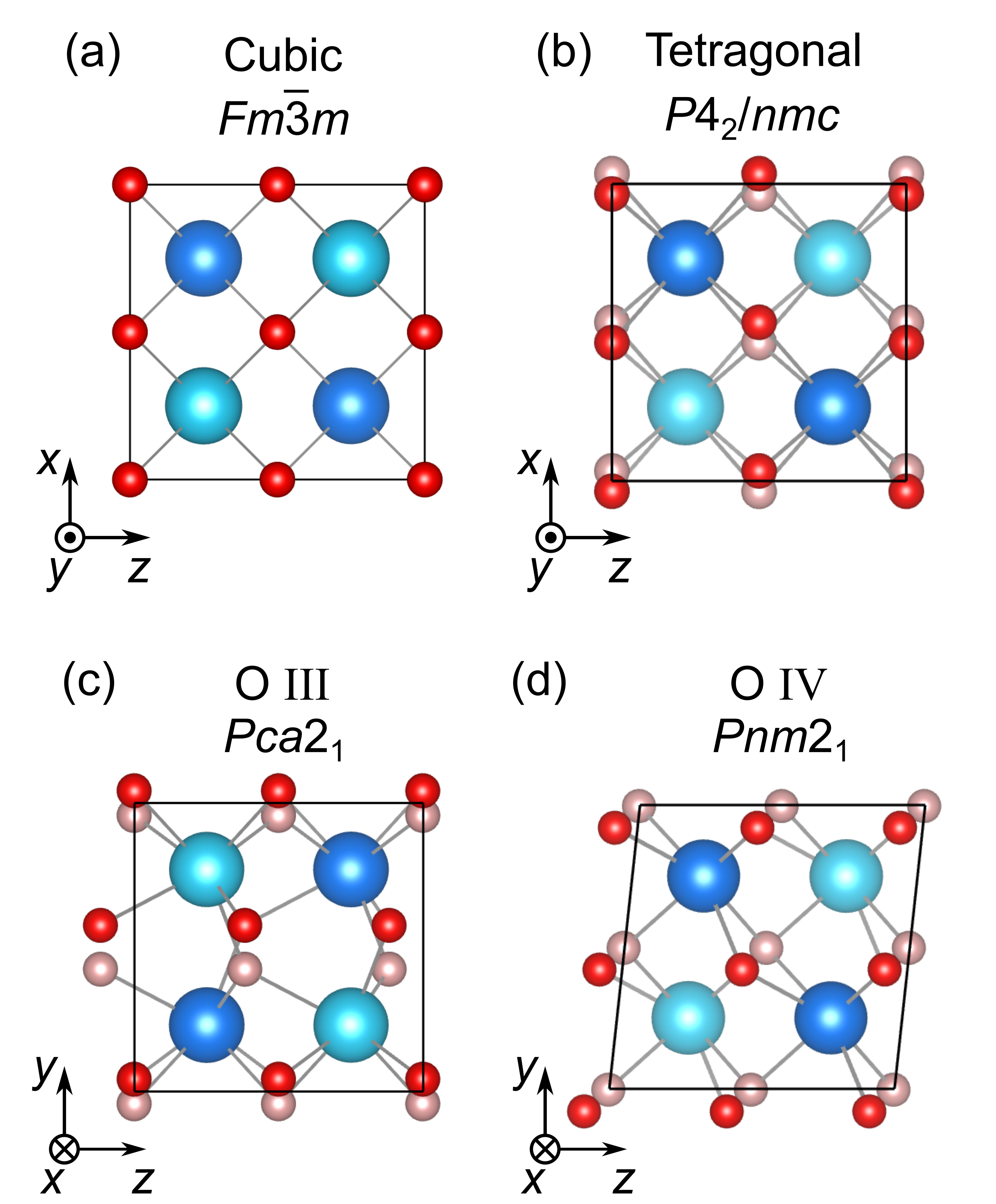
Figure 1: (a) Cubic, (b) tetragonal, (c) oIII and (d) oIV phases of HfO₂. Along the viewing direction, nearer and farther Hf atoms are represented by dark blue and light blue spheres, respectively. Similarly, nearer and farther O atoms are represented by red and pink spheres, respectively.

In this paper, we report the results of first-principles calculations for HfO₂ and substitutional derivatives (Y doped HfO₂ and Hf_0.5Zr_0.5O₂), with the construction of their energy landscapes as a function of selected symmetry–adapted lattice modes. Specifically, we consider uniform electric fields applied in various directions with respect to the crystal axes and map out the structural evolution and hysteresis loops for selected electric field profiles. We find that Y and Zr substitution modifies the energy landscape of pure HfO₂. In particular, the substitutions change the minimum barrier path from the nonpolar tetragonal to the ferroelectric oIII phase and between up and down ferroelectric variants. These results lead to a better understanding of wake–up and switching behavior in these systems, enabling electric–field control of competing phases in HfO₂ and its derivatives.

II Methods

We carry out Density functional theory (DFT) calculations with the Quantum–espresso Giannozzi et al. (2009) package for structural relaxations under finite electric fields and the ABINIT Gonze et al. (2002) package for structure optimizations with fixed lattice modes. Optimized norm–conserving local density approximation (LDA) pseudopotentials were generated using the Opium package Opi ; Bennett (2012). A 4$\times$4$\times 4$ Monkhorst–Pack $k$–point mesh was used to sample the Brillouin zone for the conventional 12–atom cell with corresponding meshes for the supercells. The plane–wave cutoff energy was 50 Ry Monkhorst and Pack (1976). Structural relaxations were performed with a force threshold of 5.0$\times 10^{-6}$ Hartree per Bohr. Relaxed structural parameters for the various bulk phases of pure HfO₂ are reported in supplementary materials (SM) section I. The computed lattice constants are identical to those in our previous work Reyes-Lillo et al. (2014) and are in good agreement with the results in other studies.

Here, we consider pure HfO₂ and two substitutional derivatives: Y doped HfO₂ (Y–HfO₂) and Hf_0.5Zr_0.5O₂, as shown in Fig. 2. The conventional unit cell of pure HfO₂ contains 12 atoms or 4 formula units [Fig.2 (a)]. For Y–HfO₂, we double this unit cell along the $y$ axis and substitute one of the Hf atoms by an Y atom, corresponding to a 12.5 % doping concentration [Fig. 2 (b)]. For Hf_0.5Zr_0.5O₂, we consider a structure with 1:1 layered cation ordering, as shown in Fig. 2 (c). Previous experimental work has shown that this superlattice structure with alternating Zr and Hf cation layers exhibits electrical behavior quite similar to that of random–cation Hf_0.5Zr_0.5O₂ Weeks et al. (2017).

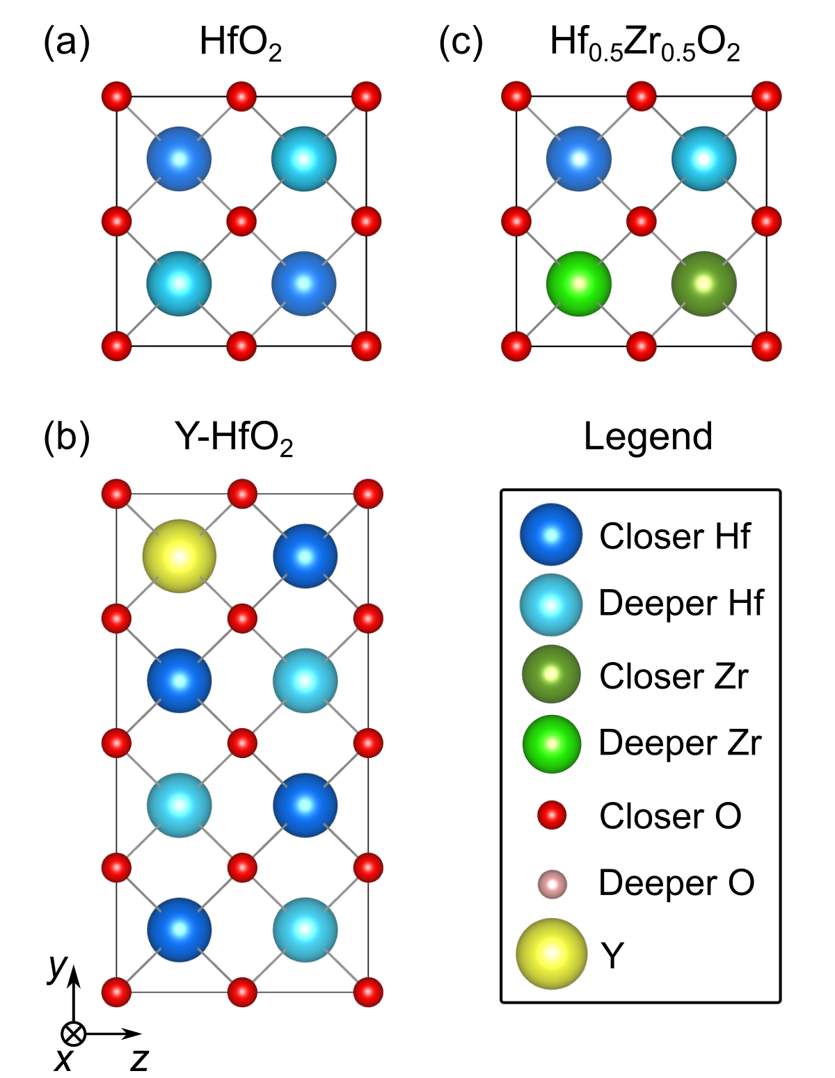
Figure 2: High–symmetry cubic structures of the (a) bulk HfO₂, (b) Y doped HfO₂, and (c) Hf_0.5Zr_0.5O₂ unit cells. Hf, Zr, O and Y atoms are represented by blue, green, red and yellow spheres respectively. As in Fig. 1, the darkness of the color indicates the spatial distance along the view direction; closer atoms are represented by dark colors, which farther ones are represented by light colors.

We describe the low–symmetry structures in each system by homogeneously straining them back to the lattice of the ideal cubic fluorite reference structure and decomposing the atomic displacements from the reference structure into the symmetry–adapted lattice modes of the reference structure Lee et al. (2020); Reyes-Lillo et al. (2014). The atomic displacement patterns of the lattice modes and the method for calculating the mode amplitudes are described in SM section II. In TABLE S6, the lattice–mode patterns and amplitudes relevant to the optimized tetragonal, oIII and oIV phases are listed. The oxygen atom positions in the tetragonal structure are obtained from an anti–polar $X_{2}^{-}$ mode, with displacements of oxygen chains along the 4–fold direction, here taken as the $x$ direction, alternating in a 2D checkerboard pattern [Fig. S1(a)]. Starting from the tetragonal structure, the polar phases are generated by the 3–fold–degenerate zone–center polar $\Gamma^{-}_{4}$ mode, corresponding to uniform displacement of the Hf atoms relative to the simple cubic oxygen network (Fig. S1(c)). We refer to these modes as $\Gamma_{x}$, $\Gamma_{y}$ and $\Gamma_{z}$, with amplitudes $u_{x}$, $u_{y}$ and $u_{z}$, respectively. The oIII structure, whose polarization is along the [001] direction, has only one non–zero polar mode amplitude $u_{z}{\neq}\ 0$. In the oIV structure, $u_{y}=u_{z}{\neq}\ 0$, indicating a [011]–directed polarization.

The polarization can be estimated from the linear dependence of polarization $P$ on the amplitude of the polar mode in the high–symmetry reference structure as Rabe et al. (2007)

$$P_{i}=\frac{e}{\Omega}Z^{*}u_{i},$$ (1)

where $i=x,y,z$, $e$ is the electronic charge, $\Omega$ is the volume of the supercell, and $Z^{*}$ is the mode Born effective charge (SM section III).

There are two relevant components of the anti–polar $X_{5}^{+}$ mode. The $X_{5,y}^{+}({\bm{q}}\parallel{\bm{\hat{x}}})$ mode, with amplitude $A_{y}$, describes the displacement of oxygen layers along the $y$ axis, alternating in the $x$ direction, as shown in Fig. S1 (d). This amplitude is nonzero both in the oIII and oIV structures. The $X_{5,z}^{+}({\bm{q}}\parallel{\bm{\hat{y}}})$ mode, with amplitude $B_{z}$, describes the displacement of oxygen layers along the $z$ axis, alternating in the $y$ direction, as shown in Fig. S1 (c). This amplitude is nonzero only in the oIII structure. $B_{z}$ and $u_{z}$ combine to give zero and non–zero oxygen displacements in alternating layers in the oIII structure.

For constructing the energy landscape as a function of the lattice–mode amplitudes, we generate structures with selected amplitudes of the lattice modes, and then, by using the ABINIT package, relax the structures with the constraint that the selected mode amplitudes stay fixed while the amplitudes of other modes compatible with the resulting symmetry are optimized (SM section III). In certain cases to be discussed below, when the lattice mode amplitude is zero, the structure is relaxed with the lower symmetry corresponding to a small nonzero value of the lattice mode amplitude. This ensures that the energy plotted as a function of lattice amplitude is continuous through zero amplitude, which would not in general be the case if the zero-amplitude energy were computed at a saddle point protected by high symmetry. Then, we fit the calculated energies with Landau polynomials with the lattice–mode amplitudes as order parameters, and use the polynomials to generate the energy landscapes.

We determine the effects of uniform applied electric field by relaxing the structure with added forces ${\bm{F}_{i}}$ on the ions: ${\bm{F}_{i}}=Z_{i}^{*}e\cdot{{\bm{E}}}$, where $Z^{*}_{i}$ is the effective charge tensor of ion $i$ and ${\bm{E}}$ is the applied electric field (SM section III). To construct electric–field hysteresis loops, an electric field cycle is applied to each of the systems considered with the tetragonal structure as the initial state. In each cycle, we fix a direction for the electric field and then increase the magnitude of the electric field in steps from 0 to $+E_{max}$ in steps, then decrease it to $-E_{max}$, and then increase it again to $+E_{max}$. Here, $E_{max}=13.5$ MV/cm is the maximum electric field that the HfO₂ crystal can sustain in our DFT calculations. Beyond $E_{max}=13.5$, the system becomes ionically conductive and the crystal crashes. The step size is $\Delta{E}=1.5$ MV/cm, except near the critical electric field at which switching occurs, where $\Delta{E}$ is reduced to 0.5 MV/cm. For each value of $E$, the optimized structure from the previous step is used as the starting structure for relaxation. Hysteresis loops are plotted showing the polar–mode amplitudes of the optimized structures as a function of electric field.

The lattice–mode–amplitude energy landscape can be used to understand the electric–field cycling behaviors to first order in the field. To see this, we start with a given nonzero electric field and relax the structure as described above. Next, the resulting structure is relaxed at zero field, constraining the values of $u_{y}$ and $u_{z}$, to determine one point in the lattice–mode–amplitude energy landscape. We find that the amplitudes of the nonpolar modes in the structure relaxed under a nonzero electric field, and in the structure computed with a zero electric field and constrained values of $u_{y}$ and $u_{z}$, are the same to a good approximation. Therefore, the effect of nonzero field can be described by adding a term $-P{\cdot}E$, where $P$ is the spontaneous polarization Sai et al. (2002), to the computed zero-field energy landscape.

III Results

We begin by considering the energy landscape of pure HfO₂ in zero applied field, identifying the local minima that correspond to competing phases and analyzing the barriers that separate them. We then present results for electric–field hysteresis loops of pure HfO₂, focusing on the structural changes and switching behavior as the magnitude of the field changes. Finally, we extend our discussion to the Y–HfO₂ and Hf_0.5Zr_0.5O₂ systems, and show how Y and Zr substitutions change the energy landscape and electric–field cycling behaviors.

III.1 Pure HfO₂

The energy landscape of pure HfO₂ as a function of the two polar mode amplitudes $u_{y}$ and $u_{z}$ is shown in Fig. 3 (a). There are three types of local minima, corresponding to the tetragonal, oIII, and oIV phases. The optimal path from the tetragonal phase to the oIII phase runs along the horizontal axis, with the optimal value of $u_{y}$ at each $u_{z}$ being zero. Similarly, the optimal path from the tetragonal phase to the oIV phase runs along the line $u_{y}=u_{z}$.

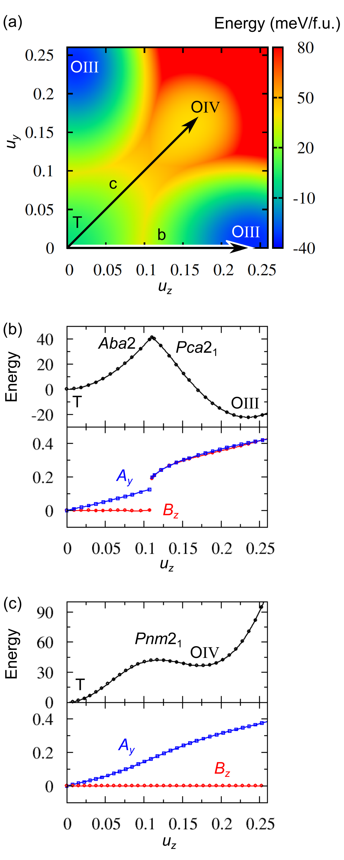
Figure 3: (a) Energy landscape of HfO₂ as a function of $u_{y}$ and $u_{z}$; We focus on the two paths indicated by the arrows. (b) Energy, $A_{y}$, and $B_{z}$ as a function of $u$ along the path b from the tetragonal to the oIII phase. Dots are calculated points and the solid line is an interpolation. (c) Energy, $A_{y}$, and $B_{z}$ as a function of $u$ along the path c from the tetragonal to the oIV phase.

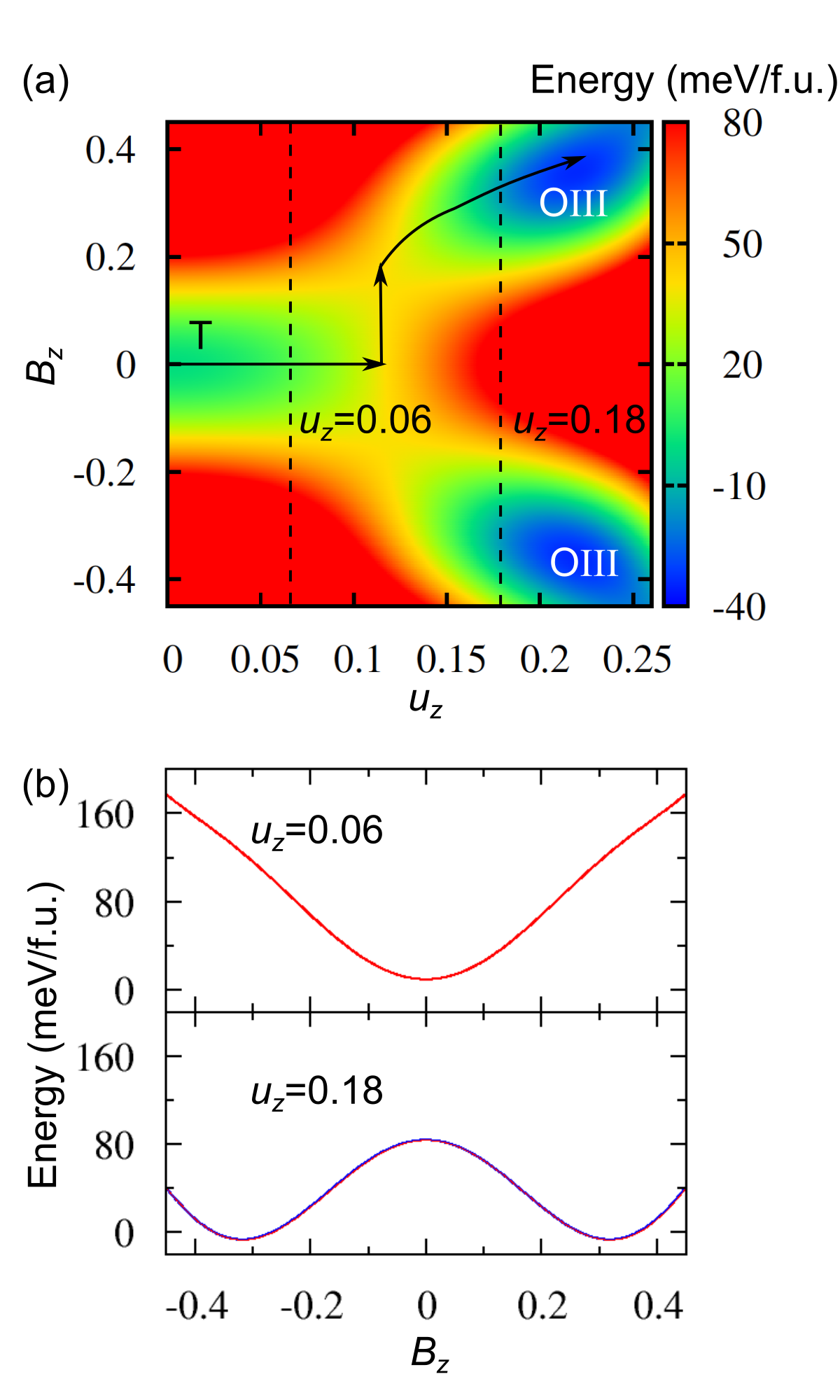
Figure 4: (a) Energy landscape of HfO₂ as a function of $u_{z}$ and $B_{z}$ (b) Energy as a function of $B_{z}$, for $u_{z}$ smaller and larger than the critical value 0.12 Å  respectively.

The nature of the barriers between the local minima can be understood by plotting the energy and the relaxed amplitudes $A_{y}$ and $B_{z}$ of the $X_{5}^{+}$ modes (Fig. S1) for two straight–line paths in ($u_{z}$,$u_{y}$) space, as shown in Fig. 3 (b) and Fig. 3 (c). Along the straight line path ($u$,0⁺) [Fig. 3 (b)], a cusp at $u=0.12$ Å  separates the two local minima corresponding to the tetragonal and oIII phases, with a change in space group symmetry from $Aba2$, for the tetragonal phase with a constrained polar distortion, to $Pca2_{1}$, for the oIII phase. In the $Aba2$ phase, the mode amplitude $A_{y}$ grows linearly with $u$, while $B_{z}$ remains zero [Fig. 3 (b) and Fig. S1 (b)]. In the $Pca2_{1}$ phase, found for $u>0.12$ Å, $A_{y}\ \approx\ B_{z}\neq 0$, with jumps in both $A_{y}$ and $B_{z}$ across the cusp. The jump in $B_{z}$ can be understood by plotting the energy landscape as a function of $u_{z}$ and $B_{z}$, with other symmetry–allowed modes, including $A_{y}$, allowed to relax [Fig. 4 (a)]. For $u_{z}<0.12$ Å, the energy as a function of $B_{z}$ has a single minimum at $B_{z}$=0, while for $u_{z}>0.12$ Å, it is a double well [Fig. 4 (b)].

To understand the nature of the barrier between the tetragonal phase and the oIV phase, we show the energy and the mode amplitudes $A_{y}$ and $B_{z}$ as a function of $u$ along the straight–line path ($u,u$) connecting the tetragonal phase to the oIV phase [Fig. 3 (b)]. Nonzero $u$ lowers the symmetry to $Pnm2_{1}$. With increasing $u$, $A_{y}$ grows linearly with $u_{z}$ and $B_{z}$ remains zero. The $Pnm2_{1}$ oIV phase is metastable, with an energy of 31 meV/f.u. above the tetragonal phase. The energy barrier from the oIV phase is only 6 meV/f.u. and is smooth rather than cusp–like.

To investigate the electrical field cycling behavior, we applied two electric field cycles to the tetragonal phase, one with electric field along the [001] direction and the other along [011]. The polar–mode–amplitude hysteresis loops are shown in Fig. 5 (a) and the evolution of the free energy landscape with electric field is shown in Figs. S4 and S5. For $\bm{E}//$[001], a tetragonal to polar oIII phase transition occurs at $E_{\rm{T}{\rightarrow}{\rm{P}}}=11$ MV/cm. After the electric field is returned to zero, the system is trapped at the local minimum corresponding to the oIII structure. As the electric field becomes more negative, the polarization switches at $E_{\rm{P}{\rightarrow}-{\rm{P}}}=-13$ MV/cm. Note that after the initial transition to the oIII phase, field cycling switches the system back and forth between up and down variants as in a conventional ferroelectric. For $\bm{E}//$[011], the critical field for inducing a tetragonal to polar oIV phase transition is $E_{\rm{T}{\rightarrow}{\rm{P}}}=7$ MV/cm. After the electric field is returned to zero, the system is trapped at the local minimum corresponding to the oIV structure. As the electric field becomes more negative, this local minimum disappears and at $E_{\rm{P}{\rightarrow}{\rm{T}}}=-2.5$ MV/cm, the system switches back to the tetragonal phase. With further increase of the electric field in the negative direction, the polarization switches at $E_{\rm{P}{\rightarrow}-{\rm{P}}}=-7$ MV/cm.

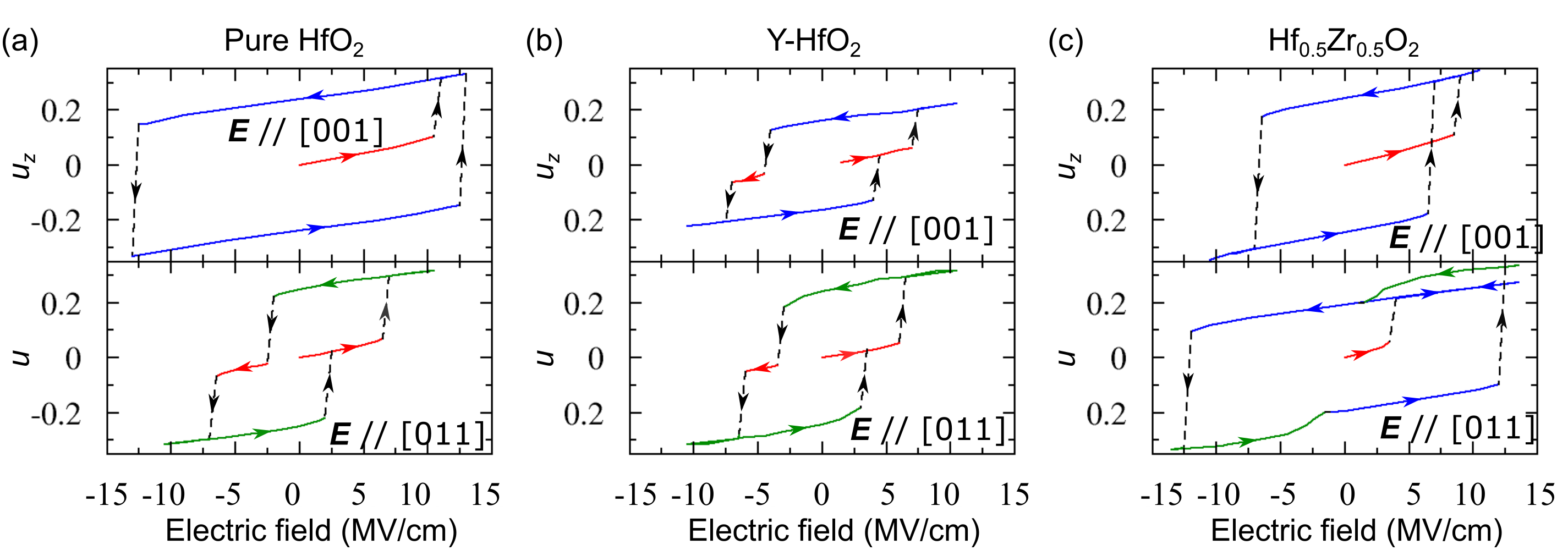
Figure 5: Hysteresis loops of (a) pure HfO₂, (b) Y–HfO₂ and (c) Hf_0.5Zr_0.5O₂, with electric field along [001] and [011] directions respectively. The evolution of the free energy landscape with electric field is shown in SM section V. In pure HfO₂, the critical field for polarization flipping ($E_{\rm{P}{\rightarrow}-{\rm{P}}}=-13$ MV/cm) is very close to the maximum electric field which the crystal can sustain ($E_{max}=13.5$ MV/cm). In the cases with ${\rm{E}}//[011]$, $u$ represents the magnitude of the polar modes projected on the direction of the electric field. The color of the segment (red, blue and green) indicates the state is in the local minimum corresponding to the tetragonal, oIII, oIV structure respectively. For Y–HfO₂, the blue segment represents that the structure containing an oIII part.

III.2 Y–HfO₂

The Y–doped HfO₂ 1$\times$2$\times$1 supercell is shown in Fig. 2 (b). The arrangement of Y atoms considered respects tetragonal symmetry, so that relaxing the structure from the high–symmetric cubic phase gives rise to a nonpolar tetragonal structure quite similar to the tetragonal structure of HfO₂, with nonzero values for the $X_{2}^{-}$ mode. Here, we would like to note that for the phases we study, we find that heterovalent Y doping adds a hole at the top of he valence band without introducing any states in the gap, which is consistent with Ref. Lee et al. (2008).

The energy of Y–HfO₂ as a function of $u_{z}$ is shown in Fig. 6 (a), where we see three phases separated by cusps, with one local minimum at $u_{z}=0$ Å and a second at $u_{z}=0.17$ Å. Relative to pure HfO₂, both the value of $u_{z}$ at the first cusp and the height of the energy barrier separating the two local minima are lower in Y–HfO₂. For values of $u_{z}$ below the first cusp value $u_{z}<0.06$ Å, the energy as a function of $u_{z}$ is very close to that of pure HfO₂. In both systems, with increasing $u_{z}$, $A_{y}$ couples with $u_{z}$ linearly and $B_{z}$ remains zero. At the first cusp $u_{z}=0.06$ Å, both $A_{y}$ and $B_{z}$ exhibit boosts, indicating a structural transformation with a change in symmetry. A representative structure with $u_{z}=0.08$ Å is shown in Fig. 6 (b). The supercell can be divided into two parts with distinct behavior. The unsubstituted part of the supercell has the atomic displacements characteristic of the polar oIII structure, which is responsible for the ferroelectricity. Here, the adjacent oxygen layers (indicated by the arrows) have different bonding environments. As a result, they are prone to have different displacements, leading to a non–zero $B_{z}$, which is the character of the oIII structure. The part of the supercell containing the Y atom is less distorted. At the second cusp $u_{z}=0.10$ Å, there is a downward jump in $B_{z}$, indicating another phase transition. Fig. 6 (b) shows the structure of the polar phase at $u=u_{min}=0.18$ Å. The structure in the unsubstituted part of the supercell closely resembles the polar oIII structure, while the part of the supercell containing the Y atom is close to the oIV phase. The decrease in $B_{z}$ is attributed to the formation of the oIV phase in the Y-substituted part, with zero $B_{z}$ as indicated in Fig. 3 (c).

Relative to pure HfO₂, both the value of $u_{z}$ at the cusp and the height of the energy barrier in Y–HfO₂ are lower. indicating a smaller critical electric field $E_{\rm{T}{\rightarrow}{\rm{P}}}$ for triggering the tetragonal to polar phase transition. The behavior in applied electric field exhibits corresponding differences. The detailed evolution of the free energy landscape with electric field is shown in Fig. S6. Here, because of the added hole, the density of states at the Fermi level is nonzero and we investigate the change of structure under an electric field with an accompanying nonzero field–induced current. As shown in Fig. 5 (b), for ${\rm{E}}//[001]$, the critical field $E_{\rm{T}{\rightarrow}{\rm{P}}}=7.5$ MV/cm for the transition from the tetragonal to the polar phase is much reduced compared with that [$E_{\rm{T}{\rightarrow}{\rm{P}}}=11$ MV/cm] in pure HfO₂, as expected from the lower barrier. Futhermore, the saturation polarization is smaller than in pure HfO₂.

Fig. 7 shows the energy profile of Y–HfO₂ as a function of $u=u_{y}=u_{z}$. For small $u$, $A_{y}$ couples with $u_{z}$ linearly while $B_{z}$ remains approximately zero, very close to the behavior in pure HfO₂. Similar to the energy profile of Y–HfO₂ along the [001] direction, Y doping also introduces intermediate states, here two rather than one, and the phase changes along the transformation path are indicated by the singular points of the $B_{z}$ profile (see SM Fig. S3 for the representative structure of each intermediate state). Even though the relative energy of the oIV structure is lowered in Y–HfO₂, we see that the curvatures of the local minima, which correlate to the maximum slopes in the energy profile, are approximately the same as those in pure HfO₂, indicating that the critical fields for inducing the phase transitions are similar [Fig. 5 (a) and (b)].

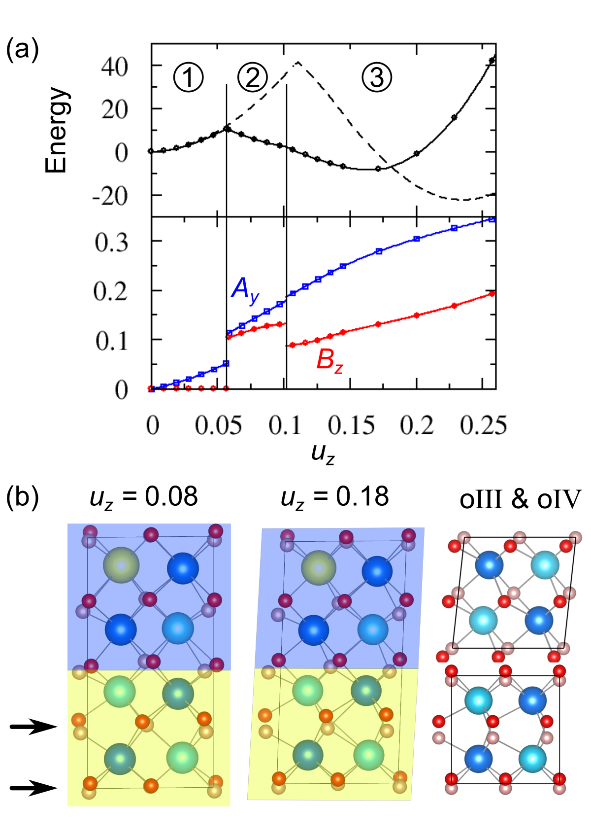
Figure 6: (a) Energy of Y–HfO₂ as a function of $u_{z}$ with other degrees of freedom relaxed. The same profile for pure HfO₂ is also plotted (dashed line) for comparison. (b) Crystal structure of Y–HfO₂ for $u_{z}$=0.08 and 0.18 Å. The structures of the oIII and oIV phase in pure HfO₂ are also shown for comparison.

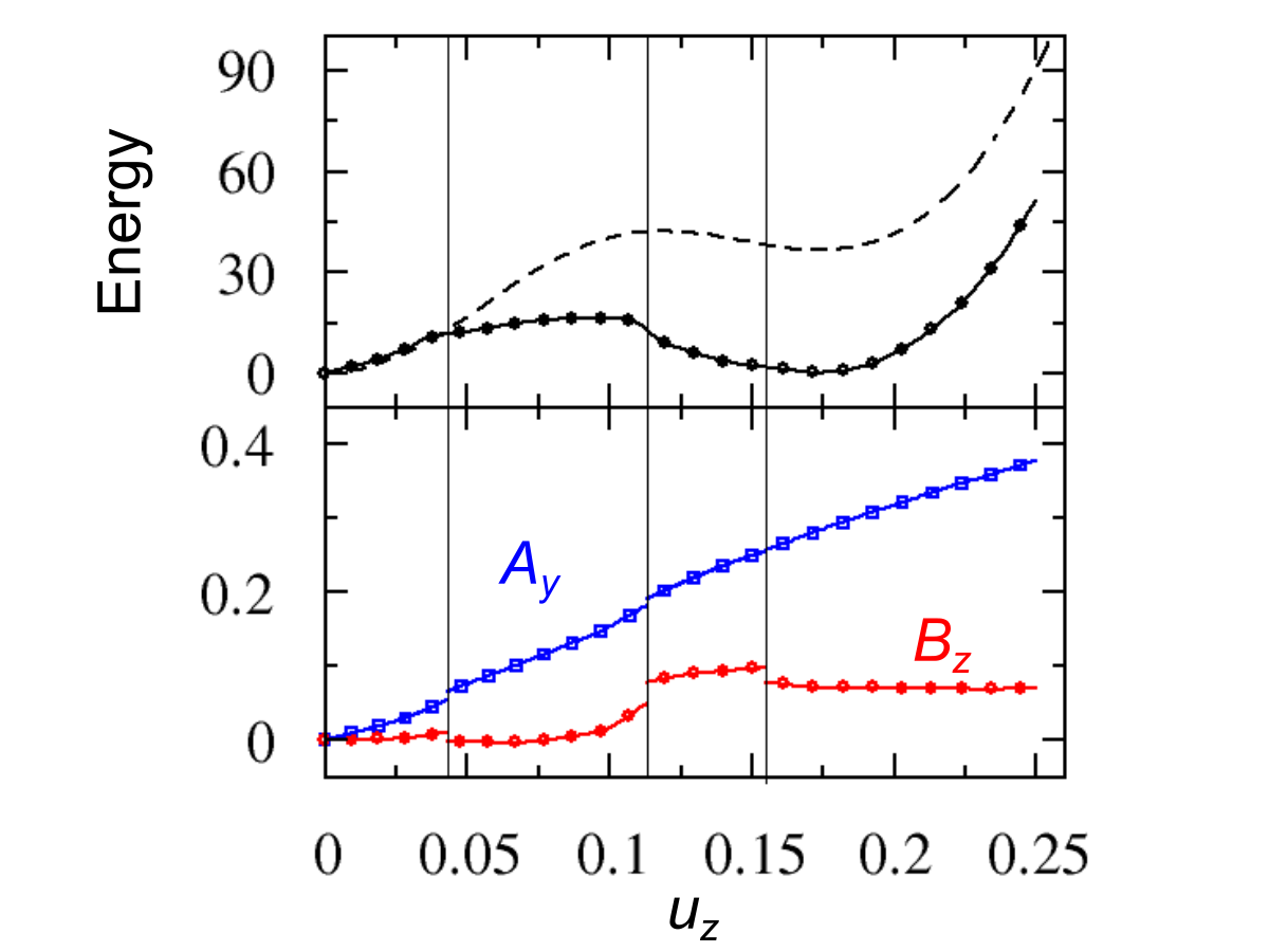
Figure 7: Energy, $A_{y}$, and $B_{z}$ as a function of $u_{z}$ along the path of the tetragonal to oIV phase transition. Along this transformation path, $u_{y}$ is fixed to be equal to $u_{z}$. The representative structures of each intermediate states are shown in Fig. S3.

III.3 Hf_0.5Zr_0.5O₂

The energy landscape of Hf_0.5Zr_0.5O₂ as a function of the two polar mode amplitudes $u_{y}$ and $u_{z}$ is shown in Fig. 8 (a). As in pure HfO₂, there are local minima corresponding to the tetragonal and oIII phases. However, the cation layering normal to the $y$ direction breaks the $y$–$z$ symmetry of pure HfO₂, so the two local minima for oIII, with polarization in the y direction and polarization in the $z$ direction respectively, are not equivalent. In addition, the polarization of z–polarized oIII polarized in the $z$ direction has a small nonzero $y$ component, which resulting in two symmetry–related variants, one with positive $y$ component and one with negative $y$ component. We also see that in Hf_0.5Zr_0.5O₂, the oIV phase is unstable. Structural optimization starting from an oIV structure leads to the oIII minimum, as shown in Fig. 8 (a).

In Fig. 8 (b), we plot the energy of Hf_0.5Zr_0.5O₂ as a function of $u_{z}$, with the amplitudes of other modes at their optimized values, shown in Fig. 8 (a) and (b). As in pure HfO₂, this energy profile also exhibits two local minima corresponding to the tetragonal and oIII phases, very little changed from the pure case. However, the cusp seen in pure HfO₂ is cut off, substantially lowering the energy barrier between the two phases. The lowering of the energy barrier results from the change in the path through the energy landscape, which goes through the oIV phase region, and around the peak between the tetragonal and oIII phase [see Fig. 8 (a)]. This is in contrast to pure HfO₂, in which the optimal path runs along the horizontal axis.

These features significantly influence the electric–field cycling behavior of Hf_0.5Zr_0.5O₂. As shown in Fig. 5 (c), both [001] and [011] directed electric fields induce a transition from the tetragonal phase to the $z$–polarized oIII phase, with the critical field $E_{\rm{T}{\rightarrow}{\rm{P}}}$ being much smaller if $E$ is applied along the [011] direction (3.5 MV/cm vs. 9 MV/cm). Furthermore, the hysteresis loop for $E//[011]$ exhibits a complex and unconventional shape. Once an [011]–directed electric field has induced the tetragonal to $z$–polarized oIII phase transition, the system stays trapped in the local oIII minimum as the field is increased to $E=13.5$ MV/cm and then decreased. However, when the electric field in the reverse direction reaches $E=-12.5$ MV/cm, the polarization switches to the [011] direction to align with the field driving the system into the oIV phase polarized in the [0$\bar{1}\bar{1}$] direction. As the magnitude of the field is decreased, the system remains trapped in the local oIV minimum until the field reaches $-1$ MV/cm, at which point the system switches back to the oIII phase with polarization in the negative $z$–direction. In Fig. S8, we show this in more detail, connecting the complexity in the hysteresis loop of Hf_0.5Zr_0.5O₂ to the specific features of its energy landscape.

The surprising fact that the critical field for switching to the oIII phase is lower along [011] than along the polarization direction [001] is related to the complexity of the energy landscape. Indeed, an electric field along [01$\bar{1}$] is also more effective in driving the state out of the oIII minimum, compared with a [00$\bar{1}$] or [0$\bar{1}\bar{1}$] oriented one. In Fig 8(c), we show the polar mode amplitude hysteresis loop for an electric field cycle in which the field is first increased from zero along [011], decreased to zero, and then increased along [01$\bar{1}$]. Because the energy landscape is the same under $u_{z}{\to}-u_{z}$, the hysteresis loop is symmetrical. The magnitude of the coercive field for flipping the polarization is 6.5 MV/cm, smaller than those (7 and 12.5 MV/cm) with electric field along [001] and [011] directions. These results open possibilities for improving the electrical performance of HfO₂ by modulating the direction of applied electric field.

We note that the results we have presented are based on calculations with the LDA functional. Using the generalized gradient approximation (GGA) changes the relative energy of each phase (see SM section I, TABLE S4), but does not destabilize any of the phases we considered. Therefore, the energy landscapes generated by GGA possess the same multiple local minima, with an electric field similarly inducing phase transitions between them.

IV Discussion

We have demonstrated that the tetragonal phase of HfO₂ can transform to the ferroelectric oIII or oIV phase under an electric field, providing insights into the emergence of ferroelectricity and electric-field-cycling behaviors. In the following subsections, we will relate our computational results to experimental observations.

IV.1 Wake–up and ferroelectricity

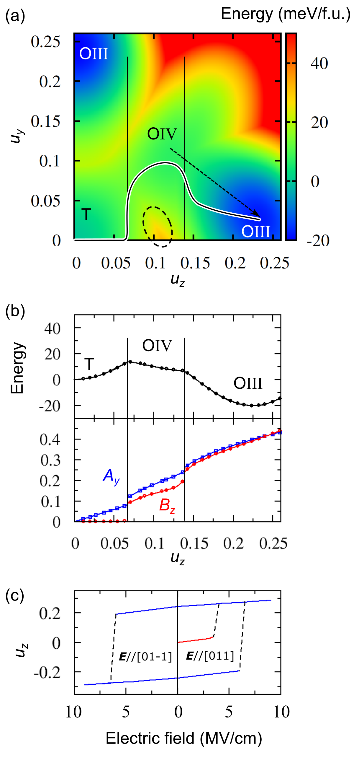
Figure 8: (a) Energy landscape of Hf_0.5Zr_0.5O₂ with respect to the amplitudes of the $u_{y}$ and $u_{z}$ polar modes; (b) Energy profiles of Hf_0.5Zr_0.5O₂ as a function of $u_{z}$，with energy minimized with respect to $u_{y}$. The values of $u_{y}$ at each $u_{z}$ are shown by the black curve with a white edge in (a). The values of $A_{y}$ and $B_{z}$ at each $u_{z}$ are shown in the lower panel. (c) Hysteresis loop in which the forward electric is along the [011] direction, and the backward one is along [01-1].

The wake–up effect, which refers to the fact that an as–grown HfO₂–based thin film needs several electric field cycles to establish its full value of switching polarization, has been widely observed in experiments Zhou et al. (2013); Pešić et al. (2016); Grimley et al. (2016); Martin et al. (2014). This wake–up effect has been attributed to various factors, including structural change at the interface Hoffmann et al. (2015a); Grimley et al. (2016); Pešić et al. (2016), and the internal bias fields caused by oxygen vacancies  Schenk et al. (2015, 2014); Mart et al. (2019).

In addition, an electric–field–induced nonpolar to polar phase transition is expected to play a significant role Pešić et al. (2016); Hoffmann et al. (2015b); Park et al. (2015b); Batra et al. (2017). In experiments, doped HfO₂ films are usually deposited at high temperature Böscke et al. (2011a, b); Mueller et al. (2012a); Müller et al. (2012). High temperature, surface energy and dopants all promote the formation of the tetragonal phase Batra et al. (2016); Lee et al. (2008). Upon cooling, the thin films can be kinetically trapped in the tetragonal phase, since it is metastable, with no unstable phonon modes Reyes-Lillo et al. (2014). However, the oIII structure has a lower energy than the nonpolar tetragonal phase, so that once the more stable oIII structure is induced by an electric field, a electric field opposite to the polarization will tend to flip the polarization to the corresponding oIII phase rather than drive the system back to the tetragonal phase.

In our calculations, for pure HfO₂ the critical electric field $E_{\rm{T}{\rightarrow}{\rm{P}}}$ for triggering this phase transition is 11 MV/cm. Our calculations also show that Y and Zr doping can cut off the cusp in the energy profiles by introducing intermediate states, and thus lower the energy barrier and critical fields ($E_{\rm{T}{\rightarrow}{\rm{P}}}=7.5$ MV/cm in Y–HfO₂ and 4 MV/cm in Hf_0.5Zr_0.5O₂). Moreover, we note that since the energy barriers are not very high, thermal vibration can facilitate the phase transition and further lower the critical fields. With the simple assumption that a phase transition will be driven by thermal vibration if (1) compared with the current state, the energy of another state is lower by more than $k_{B}T/2$ per formula unit, and (2) the energy barrier between the two states is lower than $k_{B}T/2$ per formula unit, we find that the critical fields are further reduced to 1.1 MV/cm (in Y–HfO₂) and 2.2 MV/cm (in Hf_0.5Zr_0.5O₂), which are the same order of magnitude as the experimental values Böscke et al. (2011b, a); Müller et al. (2012).

IV.2 Multiple jumps in the $P$–$E$ loop

In a conventional ferroelectric hysteresis loop, the polarization jumps at the coercive field. However, in HfO₂ based thin films, jumps in polarization can occur at two or more values of the electric field, leading to an irregular shape of the $P$–$E$ loop (as in Fig. 5). This phenomenon has been discussed in Ref. Schenk et al. (2014), and referred as the ‘split–up’ effect. This ‘split–up’ effect has been attributed to the different activation energies in grains with different oxygen vacancy concentrations Schenk et al. (2014). Here, we would like to point out that the competing phases in the energy landscape can also contribute to this effect. As shown in Fig. 5, state hopping between different (tetragonal, oIII and oIV) local minima can lead to multiple boosts. Moreover, our results demonstrate that electric field cycling behaviors are also field–direction dependent. In HfO₂-based thin films composed of multiple grains Grimley et al. (2016); Hoffmann et al. (2016); Martin et al. (2014), grains with different lattice orientations may follow different transformation paths with different critical fields.

V Conclusion

In this study, we investigated the energy landscapes of pure HfO₂, Y–doped HfO₂, and Hf_0.5Zr_0.5O₂ as a function of the polar modes $u_{y}$ and $u_{z}$. The complex energy landscapes of these systems are found to possess multiple local minima, corresponding to the tetragonal, oIII, and oIV phases respectively. Moreover, we find that Y and Zr doping can lower the energy barriers between the non–polar tetragonal phase and the ferroelectric oIII phase, by introducing intermediate states. In Hf_0.5Zr_0.5O₂ with an ordered cation arrangement, the oIV phase becomes unstable, and a new transformation path for the tetragonal to oIII phase transition is opened, with a lower energy barrier. We connect our results to experimental observations, such as the wake–up effect and $P$–$E$ loop with irregular shape, and also propose dependence of behavior on the direction of applied electric field. This work provides useful insights about the origin of the ferroelectric phase in HfO₂–based films, and suggests strategies for improving their ferroelectric performance.

References

- Bohr et al. (2007) M. T. Bohr, R. S. Chau, T. Ghani, and K. Mistry, IEEE spectrum 44, 29 (2007).
- Gutowski et al. (2002) M. Gutowski, J. E. Jaffe, C.-L. Liu, M. Stoker, R. I. Hegde, R. S. Rai, and P. J. Tobin, Appl. Phys. Lett. 80, 1897 (2002).
- Böscke et al. (2011a) T. Böscke, J. Müller, D. Bräuhaus, U. Schröder, and U. Böttger, Appl. Phys. Lett. 99, 102903 (2011a).
- Böscke et al. (2011b) T. S. Böscke, S. Teichert, D. Bräuhaus, J. Müller, U. Schröder, U. Böttger, and T. Mikolajick, Appl. Phys. Lett. 99, 112904 (2011b).
- Mueller et al. (2012a) S. Mueller, C. Adelmann, A. Singh, S. Van Elshocht, U. Schroeder, and T. Mikolajick, ECS J. Solid State Sci. Technol. 1, N123 (2012a).
- Mueller et al. (2012b) S. Mueller, J. Mueller, A. Singh, S. Riedel, J. Sundqvist, U. Schroeder, and T. Mikolajick, Adv. Funct. Mater. 22, 2412 (2012b).
- Müller et al. (2011a) J. Müller, T. Böscke, D. Bräuhaus, U. Schröder, U. Böttger, J. Sundqvist, P. Kücher, T. Mikolajick, and L. Frey, Appl. Phys. Lett. 99, 112901 (2011a).
- Müller et al. (2011b) J. Müller, U. Schröder, T. Böscke, I. Müller, U. Böttger, L. Wilde, J. Sundqvist, M. Lemberger, P. Kücher, T. Mikolajick, et al., J. Appl. Phys. 110, 114113 (2011b).
- Müller et al. (2012) J. Müller, T. S. Böscke, U. Schröder, S. Mueller, D. Bräuhaus, U. Böttger, L. Frey, and T. Mikolajick, Nano Lett. 12, 4318 (2012).
- Ruh et al. (1968) R. Ruh, H. J. Garrett, R. F. Domagala, and N. M. Tallan, J. Am. Ceram. Soc. 51, 23 (1968).
- Reyes-Lillo et al. (2014) S. E. Reyes-Lillo, K. F. Garrity, and K. M. Rabe, Phys. Rev. B 90, 140103 (2014).
- Lee et al. (2020) H.-J. Lee, M. Lee, K. Lee, J. Jo, H. Yang, Y. Kim, S. C. Chae, U. Waghmare, and J. H. Lee, Science (2020).
- Sang et al. (2015) X. Sang, E. D. Grimley, T. Schenk, U. Schroeder, and J. M. LeBeau, Appl. Phys. Lett. 106, 162905 (2015).
- Park et al. (2015a) M. H. Park, Y. H. Lee, H. J. Kim, Y. J. Kim, T. Moon, K. D. Kim, J. Müller, A. Kersch, U. Schroeder, T. Mikolajick, et al., Adv. Mater. 27, 1811 (2015a).
- Huan et al. (2014) T. D. Huan, V. Sharma, G. A. Rossetti Jr, and R. Ramprasad, Phys. Rev. B 90, 064111 (2014).
- Giannozzi et al. (2009) P. Giannozzi, S. Baroni, N. Bonini, M. Calandra, R. Car, C. Cavazzoni, D. Ceresoli, G. L. Chiarotti, M. Cococcioni, I. Dabo, A. D. Corso, S. de Gironcoli, S. Fabris, G. Fratesi, R. Gebauer, U. Gerstmann, C. Gougoussis, A. Kokalj, M. Lazzeri, L. Martin-Samos, N. Marzari, F. Mauri, R. Mazzarello, S. Paolini, A. Pasquarello, L. Paulatto, C. Sbraccia, S. Scandolo, G. Sclauzero, A. P. Seitsonen, A. Smogunov, P. Umari, and R. M. Wentzcovitch, J. Phys.: Condens. Matter 21, 395502 (2009).
- Gonze et al. (2002) X. Gonze, J.-M. Beuken, R. Caracas, F. Detraux, M. Fuchs, G.-M. Rignanese, L. Sindic, M. Verstraete, G. Zerah, F. Jollet, M. Torrent, A. Roy, M. Mikami, P. Ghosez., J.-Y. Raty, and D. Allan, Comp. Mater. Sci. 25, 478 (2002).
- (18) http://opium.sourceforge.net.
- Bennett (2012) J. W. Bennett, Phys. Procedia 34, 14 (2012).
- Monkhorst and Pack (1976) H. J. Monkhorst and J. D. Pack, Phys. Rev. B 13, 5188 (1976).
- Weeks et al. (2017) S. L. Weeks, A. Pal, V. K. Narasimhan, K. A. Littau, and T. Chiang, ACS Appl. Mater. Interfaces 9, 13440 (2017).
- Rabe et al. (2007) K. M. Rabe, C. H. Ahn, and J.-M. Triscone, Physics of Ferroelectrics: A Modern Perspective (Springer–Verlag, 2007).
- Sai et al. (2002) N. Sai, K. M. Rabe, and D. Vanderbilt, Phys. Rev. B 66, 104108 (2002).
- Lee et al. (2008) C.-K. Lee, E. Cho, H.-S. Lee, C. S. Hwang, and S. Han, Phys. Rev. B 78, 012102 (2008).
- Zhou et al. (2013) D. Zhou, J. Xu, Q. Li, Y. Guan, F. Cao, X. Dong, J. Müller, T. Schenk, and U. Schröder, Appl. Phys. Lett. 103, 192904 (2013).
- Pešić et al. (2016) M. Pešić, F. P. G. Fengler, L. Larcher, A. Padovani, T. Schenk, E. D. Grimley, X. Sang, J. M. LeBeau, S. Slesazeck, U. Schroeder, et al., Adv. Funct. Mater. 26, 4601 (2016).
- Grimley et al. (2016) E. D. Grimley, T. Schenk, X. Sang, M. Pešić, U. Schroeder, T. Mikolajick, and J. M. LeBeau, Adv. Electron. Mater. 2, 1600173 (2016).
- Martin et al. (2014) D. Martin, J. Müller, T. Schenk, T. M. Arruda, A. Kumar, E. Strelcov, E. Yurchuk, S. Müller, D. Pohl, U. Schröder, et al., Adv. Mater. 26, 8198 (2014).
- Hoffmann et al. (2015a) M. Hoffmann, U. Schroeder, T. Schenk, T. Shimizu, H. Funakubo, O. Sakata, D. Pohl, M. Drescher, C. Adelmann, R. Materlik, et al., J. Appl. Phys. 118, 072006 (2015a).
- Schenk et al. (2015) T. Schenk, M. Hoffmann, J. Ocker, M. Pešić, T. Mikolajick, and U. Schroeder, ACS Appl. Mater. Interfaces 7, 20224 (2015).
- Schenk et al. (2014) T. Schenk, U. Schroeder, M. Pešić, M. Popovici, Y. V. Pershin, and T. Mikolajick, ACS Appl. Mater. Interfaces 6, 19744 (2014).
- Mart et al. (2019) C. Mart, K. Kühnel, T. Kämpfe, M. Czernohorsky, M. Wiatr, S. Kolodinski, and W. Weinreich, ACS Appl. Mater. Interfaces 1, 2612 (2019).
- Hoffmann et al. (2015b) M. Hoffmann, U. Schroeder, C. Künneth, A. Kersch, S. Starschich, U. Böttger, and T. Mikolajick, Nano Energy 18, 154 (2015b).
- Park et al. (2015b) M. H. Park, H. J. Kim, Y. J. Kim, Y. H. Lee, T. Moon, K. D. Kim, S. D. Hyun, and C. S. Hwang, Appl. Phys. Lett. 107, 192907 (2015b).
- Batra et al. (2017) R. Batra, T. D. Huan, J. L. Jones, G. Rossetti Jr, and R. Ramprasad, J. Phys. Chem. C 121, 4139 (2017).
- Batra et al. (2016) R. Batra, H. D. Tran, and R. Ramprasad, Appl. Phys. Lett. 108, 172902 (2016).
- Hoffmann et al. (2016) M. Hoffmann, M. Pešić, K. Chatterjee, A. I. Khan, S. Salahuddin, S. Slesazeck, U. Schroeder, and T. Mikolajick, Adv. Funct. Mater. 26, 8643 (2016).