Vector Projection Network for Few-shot Slot Tagging in Natural Language Understanding

Abstract

Few-shot slot tagging becomes appealing for rapid domain transfer and adaptation, motivated by the tremendous development of conversational dialogue systems. In this paper, we propose a vector projection network for few-shot slot tagging, which exploits projections of contextual word embeddings on each target label vector as word-label similarities. Essentially, this approach is equivalent to a normalized linear model with an adaptive bias. The contrastive experiment demonstrates that our proposed vector projection based similarity metric can significantly surpass other variants. Specifically, in the five-shot setting on benchmarks SNIPS and NER, our method outperforms the strongest few-shot learning baseline by $6.30$ and $13.79$ points on F₁ score, respectively. Our code will be released at https://github.com/sz128/few_shot_slot_tagging_and_NER.

1 Introduction

Natural language understanding (NLU) is a key component of conversational dialogue systems, converting user’s utterances into the corresponding semantic representations Wang et al. (2005) for certain narrow domain (e.g., booking hotel, searching flight). As a core task in NLU, slot tagging is usually formulated as a sequence labeling problem Mesnil et al. (2015); Sarikaya et al. (2016); Liu and Lane (2016).

Recently, motivated by commercial applications like Amazon Alexa, Apple Siri, Google Assistant, and Microsoft Cortana, great interest has been attached to rapid domain transfer and adaptation with only a few samples Bapna et al. (2017). Few-shot learning approaches Fei-Fei et al. (2006); Vinyals et al. (2016) become appealing in this scenario  Fritzler et al. (2019); Geng et al. (2019); Hou et al. (2020), where a general model is learned from existing domains and transferred to new domains rapidly with merely few examples (e.g., in one-shot learning, only one example for each new class).

The similarity-based few-shot learning methods have been widely analyzed on classification problems Vinyals et al. (2016); Snell et al. (2017); Sung et al. (2018); Yan et al. (2018); Yu et al. (2018); Sun et al. (2019); Geng et al. (2019); Yoon et al. (2019), which classify an item according to its similarity with the representation of each class. These methods learn a domain-general encoder to extract feature vectors for items in existing domains, and utilize the same encoder to obtain the representation of each new class from very few labeled samples (support set). This scenario has been successfully adopted in the slot tagging task by considering both the word-label similarity and temporal dependency of target labels Hou et al. (2020). Nonetheless, it is still a challenge to devise appropriate word-label similarity metrics for generalization capability.

In this work, a vector projection network is proposed for the few-shot slot tagging task in NLU. To eliminate the impact of unrelated label vectors but with large norm, we exploit projections of contextual word embeddings on each normalized label vector as the word-label similarity. Moreover, the half norm of each label vector is utilized as a threshold, which can help reduce false positive errors.

One-shot and five-shot experiments on slot tagging and named entity recognition (NER) Hou et al. (2020) tasks show that our method can outperform various few-shot learning baselines, enhance existing advanced methods like TapNet Yoon et al. (2019); Hou et al. (2020) and prototypical network Snell et al. (2017); Fritzler et al. (2019), and achieve state-of-the-art performances.

Our contributions are summarized as follows:

• We propose a vector projection network for the few-shot slot tagging task that utilizes projections of contextual word embeddings on each normalized label vector as the word-label similarity.

• We conduct extensive experiments to compare our method with different similarity metrics (e.g., dot product, cosine similarity, squared Euclidean distance). Experimental results demonstrate that our method can significantly outperform the others.

2 Related Work

One prominent methodology for few-shot learning in image classification field mainly focuses on metric learning Vinyals et al. (2016); Snell et al. (2017); Sung et al. (2018); Oreshkin et al. (2018); Yoon et al. (2019). The metric learning based methods aim to learn an effective distance metric. It can be much simpler and more efficient than other meta-learning algorithms Munkhdalai and Yu (2017); Mishra et al. (2018); Finn et al. (2017).

As for few-shot learning in natural language processing community, researchers pay more attention to classification tasks, such as text classification Yan et al. (2018); Yu et al. (2018); Sun et al. (2019); Geng et al. (2019). Recently, few-shot learning for slot tagging task becomes popular and appealing. Fritzler et al. (2019) explored few-shot NER with the prototypical network. Hou et al. (2020) exploited the TapNet and label dependency transferring for both slot tagging and NER tasks. Compared to these methods, our model can achieve better performance in new domains by utilizing vector projections as word-label similarities.

3 Problem Formulation

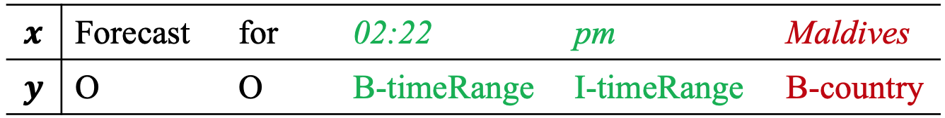
Figure 1: A data sample in domain GetWeather.

We denote each sentence $\boldsymbol{x}=(x_{1},\cdots,x_{|\boldsymbol{x}|})$ as a word sequence, and define its label sequence as $\boldsymbol{y}=(y_{1},\cdots,y_{|\boldsymbol{x}|})$. An example for slot tagging in domain GetWeather is provided in Fig 1. For each domain $\mathcal{D}$, it includes a set of $(\boldsymbol{x},\boldsymbol{y})$ pairs, i.e., $\mathcal{D}=\{(\boldsymbol{x}^{(i)},\boldsymbol{y}^{(i)})\}_{i=1}^{|\mathcal{D}|}$.

In the few-shot scenario, the slot tagging model is trained on several source domains $\{\mathcal{D}_{1},\mathcal{D}_{2},\cdots,\mathcal{D}_{M}\}$, and then directly evaluated on an unseen target domain $\mathcal{D}_{t}$ which only contains few labeled samples (support set). The support set, $S=\{(\boldsymbol{x}^{(i)},\boldsymbol{y}^{(i)})\}_{i=1}^{|S|}$, usually includes $k$ examples (K-shot) for each of N labels (N-way). Thus, the few-shot slot tagging task is to find the best label sequence $\boldsymbol{y}^{*}$ given an input query $\boldsymbol{x}$ in target domain $\mathcal{D}_{t}$ and its corresponding support set $S$,

$$\boldsymbol{y}^{*}=\arg\max_{\boldsymbol{y}}p_{\theta}(\boldsymbol{y}|\boldsymbol{x},S)$$ (1)

where $\theta$ refers to parameters of the slot tagging model, the $(\boldsymbol{x},\boldsymbol{y})$ pair and the support set are from the target domain, i.e., $(\boldsymbol{x},\boldsymbol{y})\sim\mathcal{D}_{t}$ and $S\sim\mathcal{D}_{t}$.

The few-shot slot tagging model is trained on the source domains to minimise the error in predicting labels conditioned on the support set,

$$\theta=\arg\max_{\theta}\sum_{m=1}^{M}\sum_{(\boldsymbol{x},\boldsymbol{y})\sim\mathcal{D}_{m},\ S\sim\mathcal{D}_{m}}\log p_{\theta}(\boldsymbol{y}|\boldsymbol{x},S)$$

4 Vector Projection Network

In this section, we will introduce our model for the few-shot slot tagging task.

4.1 Few-shot CRF Framework

Linear Conditional Random Field (CRF) Sutton et al. (2012) considers the correlations between labels in neighborhoods and jointly decodes the most likely label sequence given the input sentence Yao et al. (2014); Ma and Hovy (2016). The posterior probability of label sequence $\mathbf{y}$ is computed via:

$$\psi_{\theta}(\boldsymbol{y},\boldsymbol{x},S) =\sum_{i=1}^{|\boldsymbol{x}|}(f_{T}(y_{i-1},y_{i})+f_{E}(y_{i},\boldsymbol{x},S))$$

$$p_{\theta}(\boldsymbol{y}|\boldsymbol{x},S) =\frac{\text{exp}(\psi_{\theta}(\boldsymbol{y},\boldsymbol{x},S))}{\sum_{\boldsymbol{y}^{\prime}}\text{exp}(\psi_{\theta}(\boldsymbol{y}^{\prime},\boldsymbol{x},S))}$$

where $f_{T}(y_{i-1},y_{i})$ is the transition score and $f_{E}(y_{i},\boldsymbol{x},S)$ is the emission score at the $i$-th step.

The transition score captures temporal dependencies of labels in consecutive time steps, which is a learnable scalar for each label pair. To share the underlying factors of transition between different domains, we adopt the Collapsed Dependency Transfer (CDT) mechanism Hou et al. (2020).

The emission scorer independently assigns each word a score with respect to each label $y_{i}$, which is defined as a word-label similarity function:

$$f_{E}(y_{i},\boldsymbol{x},S)=\textsc{Sim}(E(\boldsymbol{x})_{i},\mathbf{c}_{y_{i}})$$ (2)

where $E$ is a contextual word embedding function, e.g., BLSTM Graves (2012), Transformer Vaswani et al. (2017), $\mathbf{c}_{y_{i}}$ is the label embedding of $y_{i}$ which is extracted from the support set $S$. In this paper, we adopt a pre-trained BERT model Devlin et al. (2019) as $E$.

Various models are proposed to extract label embedding $\mathbf{c}_{y_{i}}$ from $S$, such as matching network Vinyals et al. (2016), prototypical network Snell et al. (2017) and TapNet Yoon et al. (2019). Take the prototypical network as an example, each prototype (label embedding) is defined as the mean vector of the embedded supporting points belonging to it:

$$\mathbf{c}_{y_{i}}=\frac{1}{N_{y_{i}}}\sum_{j=1}^{|S|}\sum_{k=1}^{|\boldsymbol{x}^{(j)}|}\mathbb{I}\{y_{k}^{(j)}=y_{i}\}E(\boldsymbol{x}^{(j)})_{k}$$ (3)

where $N_{y_{i}}=\sum_{j=1}^{|S|}\sum_{k=1}^{|\boldsymbol{x}^{(j)}|}\mathbb{I}\{y_{k}^{(j)}=y_{i}\}$ is the number of words labeled with $y_{i}$ in the support set.

4.2 Vector Projection Similarity

For the word-label similarity function, we propose to exploit vector projections of word embeddings $\mathbf{x}_{i}$ on each normalized label vector $\mathbf{c}_{k}$:

$$\textsc{Sim}(\mathbf{x}_{i},\mathbf{c}_{k})=\mathbf{x}_{i}^{\top}\frac{\mathbf{c}_{k}}{||\mathbf{c}_{k}||}$$ (4)

Different with the dot product used by Hou et al. (2020), it can help eliminate the impact of $\mathbf{c}_{k}$’s norm to avoid the circumstance where the norm of $\mathbf{c}_{k}$ is enough large to dominate the similarity metric. In order to reduce false positive errors, the half norm of each label vector is utilized as an adaptive bias term:

$$\textsc{Sim}(\mathbf{x}_{i},\mathbf{c}_{k})=\mathbf{x}_{i}^{\top}\frac{\mathbf{c}_{k}}{||\mathbf{c}_{k}||}-\frac{1}{2}||\mathbf{c}_{k}||$$ (5)

4.3 Explained as a Normalized Linear Model

A simple interpretation for the above vector projection network is to learn a distinct linear classifier for each label. We can rewrite the above formulas as a linear model:

$$\textsc{Sim}(\mathbf{x}_{i},\mathbf{c}_{k})=\mathbf{x}_{i}^{\top}\mathbf{w}_{k}+b_{k}$$ (6)

where $\mathbf{w}_{k}=\frac{\mathbf{c}_{k}}{||\mathbf{c}_{k}||}$ and $b_{k}=-\frac{1}{2}||\mathbf{c}_{k}||$. The weights are normalized as $||\mathbf{w}_{k}||=1$ to improve the generalization capability of the few-shot model. Experimental results indicate that vector projection is an effective choice compared to dot product, cosine similarity, squared Euclidean distance, etc.

5 Experiment

We evaluate the proposed method following the data split  provided by Hou et al. (2020) on SNIPS Coucke et al. (2018) and NER datasets. It is in the episode data setting Vinyals et al. (2016), where each episode contains a support set (1-shot or 5-shot) and a batch of labeled samples. For slot tagging, the SNIPS dataset consists of 7 domains with different label sets: Weather (We), Music (Mu), PlayList (Pl), Book (Bo), Search Screen (Se), Restaurant (Re) and Creative Work (Cr). For NER, 4 different datasets are utilized to act as different domains: CoNLL-2003 (News) Sang and De Meulder (2003), GUM (Wiki) Zeldes (2017), WNUT-2017 (Social) Derczynski et al. (2017) and OntoNotes (Mixed) Pradhan et al. (2013). More details of the data split are shown in Appendix A.

For each dataset, we follow Hou et al. (2020) to select one target domain for evaluation, one domain for validation, and utilize the rest domains as source domains for training. We also report the average F₁ score at the episode level. For each experiment, we run it ten times with different random seeds. The training details are illustrated in Appendix B.

	Model	We	Mu	Pl	Bo	Se	Re	Cr	Avg.
1-shot	SimBERT	36.10	37.08	35.11	68.09	41.61	42.82	23.91	40.67
	TransferBERT	55.82	38.01	45.65	31.63	21.96	41.79	38.53	39.06
	L-WPZ(ProtoNet)+CDT+PWE	71.23	47.38	59.57	81.98	69.83	66.52	62.84	65.62
	L-TapNet+CDT+PWE	71.53	60.56	66.27	84.54	76.27	70.79	62.89	70.41
	L-TapNet+CDT+VP (ours)	71.65	61.73	63.97	83.34	74.00	71.91	71.02	71.09
	ProtoNet+CDT+VP (ours)	73.56	58.40	68.93	82.32	79.69	73.40	70.25	72.37
	L-ProtoNet+CDT+VP (ours)	73.19	58.62	68.26	83.54	77.88	73.48	69.54	72.07
	ProtoNet+CDT+VPB (ours)	72.65	57.35	68.72	81.92	74.68	72.48	70.04	71.12
	L-ProtoNet+CDT+VPB (ours)	73.12	57.86	69.01	82.49	75.11	73.34	70.46	71.63
5-shot	SimBERT	53.46	54.13	42.81	75.54	57.10	55.30	32.38	52.96
	TransferBERT	59.41	42.00	46.07	20.74	28.20	67.75	58.61	46.11
	L-WPZ(ProtoNet)+CDT+PWE	74.68	56.73	52.20	78.79	80.61	69.59	67.46	68.58
	L-TapNet+CDT+PWE	71.64	67.16	75.88	84.38	82.58	70.05	73.41	75.01
	L-TapNet+CDT+VP (ours)	78.25	67.79	70.66	86.17	75.80	78.51	75.93	76.16
	ProtoNet+CDT+VP (ours)	79.88	67.77	78.08	87.68	86.59	79.95	75.61	79.37
	L-ProtoNet+CDT+VP (ours)	80.26	67.81	74.62	88.16	85.79	80.41	73.84	78.70
	ProtoNet+CDT+VPB (ours)	82.91	69.23	80.85	90.69	86.38	81.20	76.75	81.14
	L-ProtoNet+CDT+VPB (ours)	82.93	69.62	80.86	91.19	86.58	81.97	76.02	81.31

Table 1: F₁ scores on few-shot slot tagging of SNIPS. Results with standard deviations is shown in Appendix C.2.

Model	1-shot					5-shot
	News	Wiki	Social	Mixed	Avg.	News	Wiki	Social	Mixed	Avg.
SimBERT	19.22	6.91	5.18	13.99	11.32	32.01	10.63	8.20	21.14	18.00
TransferBERT	4.75	0.57	2.71	3.46	2.87	15.36	3.62	11.08	35.49	16.39
L-TapNet+CDT+PWE	44.30	12.04	20.80	15.17	23.08	45.35	11.65	23.30	20.95	25.31
L-TapNet+CDT+VP (ours)	44.73	8.91	30.61	29.39	28.41	50.43	8.41	29.93	37.59	31.59
ProtoNet+CDT+VP (ours)	44.82	11.32	26.96	29.91	28.25	54.82	16.30	27.43	33.38	32.98
L-ProtoNet+CDT+VP (ours)	45.93	8.76	29.21	32.44	29.09	55.68	10.39	31.39	37.83	33.82
ProtoNet+CDT+VPB (ours)	42.50	10.78	27.17	32.06	28.13	57.42	19.48	35.06	44.45	39.10
L-ProtoNet+CDT+VPB (ours)	43.47	10.95	28.43	33.14	29.00	56.30	18.57	35.42	44.71	38.75

Table 2: F₁ scores on few-shot slot tagging of NER. Results with standard deviations is shown in Appendix C.2.

$\textsc{Sim}(\mathbf{x},\mathbf{c})$	SNIPS		NER
	1-shot	5-shot	1-shot	5-shot
$\mathbf{x}^{\top}\frac{\mathbf{c}}{||\mathbf{c}||}$	72.37	79.37	28.25	32.98
$\mathbf{x}^{\top}\frac{\mathbf{c}}{||\mathbf{c}||}-\frac{1}{2}||\mathbf{c}||$	71.12	81.14	28.13	39.10
$\mathbf{x}^{\top}\mathbf{c}$	57.92	65.03	17.10	19.91
$\frac{\mathbf{x}^{\top}}{||\mathbf{x}||}\mathbf{c}$	63.87	71.16	16.72	23.65
$\frac{\mathbf{x}^{\top}}{||\mathbf{x}||}\frac{\mathbf{c}}{||\mathbf{c}||}$	34.02	39.21	10.40	12.26
$\lambda\mathbf{x}^{\top}\mathbf{c}$	48.91	68.11	5.99	21.05
$-\frac{1}{2}||\mathbf{x}-\mathbf{c}||^{2}$	66.91	79.72	20.04	34.04

Table 3: Comparison among different similarity functions. Results are average F1-scores of all domains.

5.1 Baselines

SimBERT: For each word $x_{i}$, SimBERT finds the most similar word $x^{\prime}_{k}$ in the support set and assign the label of $x^{\prime}_{k}$ to $x_{i}$, according to cosine similarity of word embedding of a fixed BERT.

TransferBERT: A trainable linear classifier is applied on a shared BERT to predict labels for each domain. Before evaluation, it is fine-tuned on the support set of the target domain.

L-WPZ(ProtoNet)+CDT+PWE: WPZ is a few-shot sequence labeling model Fritzler et al. (2019) that regards sequence labeling as classification of each word. It pre-trains a prototypical network Snell et al. (2017) on source domains, and utilize it to do word-level classification on target domains without fine-tuning. It is enhanced with BERT, Collapsed Dependency Transfer (CDT) and Pair-Wise Embedding (PWE) mechanisms by Hou et al. (2020).

L-TapNet+CDT+PWE: The previous state-of-the-art method for few-shot slot tagging Hou et al. (2020), which incorporates TapNet Yoon et al. (2019) with BERT, CDT and PWE.

We borrow the results of these baselines from Hou et al. (2020). “L-” means label-enhanced prototypes are applied by using label name embeddings.

5.2 Main Results

Table 1 and Table 2 show results on both 1-shot and 5-shot slot tagging of SNIPS and NER datasets respectively. Our method can significantly outperform all baselines including the previous state-of-the-art model. Moreover, the previous state-of-the-art model heavily relies on PWE, which concatenates an input sentence with each sample in the support set and then feeds them into BERT to get pair-wise embeddings. By comparing “L-TapNet+CDT+PWE” with “L-TapNet+CDT+VP”, we can find that our proposed Vector Projection (VP) can achieve better performance as well as higher efficiency. If we incorporate the negative half norm of each label vector as a bias (VPB), F₁ score on 5-shot slot tagging is dramatically improved. We speculate that 5-shot slot tagging involves multiple support points for each label, thus false positive errors could occur more frequently if there is no threshold when predicting each label. We also find that label name embeddings (“L-’) help less in our methods.

5.3 Analysis

Model	SNIPS 1-shot			SNIPS 5-shot			NER 1-shot			NER 5-shot
	O-X	X-O	X-X	O-X	X-O	X-X	O-X	X-O	X-X	O-X	X-O	X-X
ProtoNet+CDT	10815	3552	17440	4802	1377	6532	58498	9890	35991	19344	1505	9091
ProtoNet+CDT+VP	4400	3409	10638	2177	1214	3610	13075	29183	13893	5217	6283	3595
ProtoNet+CDT+VPB	4118	3818	10959	1762	1076	3343	11976	26851	16032	2388	6617	3280

Table 4: Error analysis of slot tagging for different error patterns. Numbers are summed over all domains.

Ablation Study For the word-label similarity function $\textsc{Sim}(\mathbf{x},\mathbf{c})$, we also conduct contrastive experiments between our proposed vector projection and other variants including the dot product ($\mathbf{x}^{\top}\mathbf{c}$), the projection of label vector on word embedding ($\frac{\mathbf{x}^{\top}}{||\mathbf{x}||}\mathbf{c}$), cosine similarity ($\frac{\mathbf{x}^{\top}}{||\mathbf{x}||}\frac{\mathbf{c}}{||\mathbf{c}||}$), squared Euclidean distance ($-\frac{1}{2}||\mathbf{x}-\mathbf{c}||^{2}$), and even a trainable scaling factor ($\lambda\mathbf{x}^{\top}\mathbf{c}$) Oreshkin et al. (2018). The results in Table 3 show that our methods can significantly outperform these alternative metrics. We also notice that the squared Euclidean distance can achieve competitive results in the 5-shot setting. Mathematically,

$$-\frac{1}{2}||\mathbf{x}-\mathbf{c}||^{2} =-\frac{1}{2}\mathbf{x}^{\top}\mathbf{x}+\mathbf{x}^{\top}\mathbf{c}-\frac{1}{2}\mathbf{c}^{\top}\mathbf{c}$$

$$\approxeq\mathbf{x}^{\top}\mathbf{c}-\frac{1}{2}\mathbf{c}^{\top}\mathbf{c}$$

where $-\frac{1}{2}\mathbf{x}^{\top}\mathbf{x}$ is constant with respect to each label and thus omitted. It further consolidates our assumption that $\frac{1}{2}\mathbf{c}^{\top}\mathbf{c}$ can function as a bias term to alleviate false positive errors.

Effect of Vector Projection We claimed that vector projection could help reduce false positive errors. As illustrated in Figure 2, we classify all wrong predictions of slot tagging into three error types (i.e., “O-X”, “X-O” and “X-X”), where “O” means no slot and “X” means a slot tag beginning with ‘B’ or ‘I’. The error analysis of these three error types are illustrated in Table 4. We can find that our methods can significantly reduce wrong predictions of these three types in SNIPS dataset. In NER dataset, our methods can achieve a remarkable reduction in “O-X” and “X-X”, while leading to an increase of “X-O” errors. However, the total number of these three errors are reduced by our methods in NER dataset.

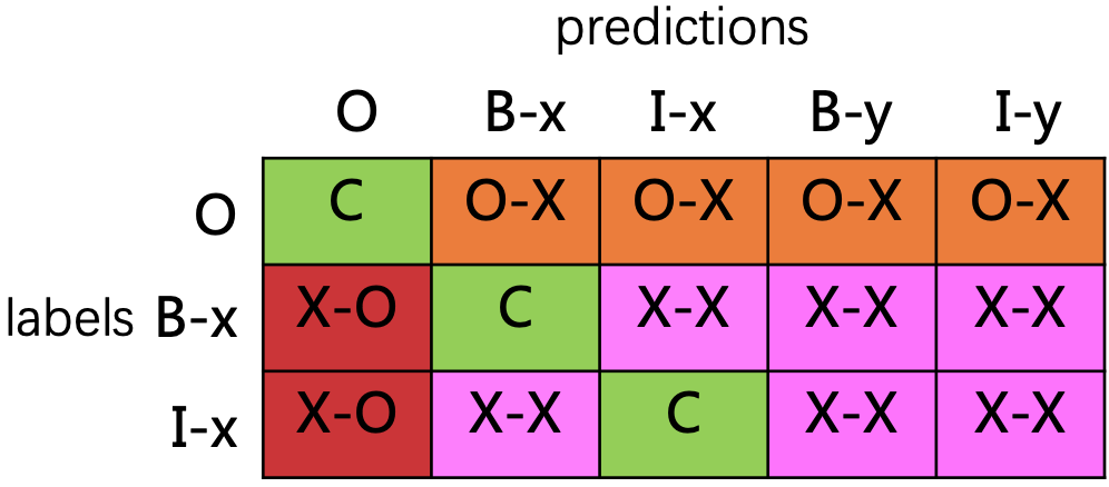
Figure 2: Definition of three error types of slot tagging, which are “O-X”, “X-O” and “X-X”. “C” means correct predictions.

Fine-tuning with Support Set Apart from the few-shot slot tagging focusing on model transfer instead of fine-tuning, we also analyze keeping fine-tuning our models on the support set in Appendix C.1.

6 Conclusion

In this paper, we propose a vector projection network for the few-shot slot tagging task, which can be interpreted as a normalized linear model with an adaptive bias. Experimental results demonstrate that our method can significantly outperform the strongest few-shot learning baseline on SNIPS and NER datasets in both 1-shot and 5-shot settings. Furthermore, our proposed vector projection based similarity metric can remarkably surpass others variants.

For future work, we would like to add a learnable scale factor for bias in Eqn. 6.

Appendix A Detail of Dataset

The data split method provided by Hou et al. (2020) are applied in SNIPS and NER datasets. Statistical analyses of the original datasets are provided in Table 5, where the number of labels (“# Labels”) is counted in inside/outside/beginning (IOB) schema.

Task	Dataset	Domain	# Sent	# Labels
Slot Tagging	SNIPS	We	2100	17
		Mu	2100	18
		Pl	2042	10
		Bo	2056	12
		Se	2059	15
		Re	2073	28
		Cr	2054	5
NER	CoNLL	News	20679	9
	GUM	Wiki	3493	23
	WNUT	Social	5657	13
	OntoNotes	Mixed	159615	37

Table 5: Statistics of original dataset.

Hou et al. (2020) reorganized the dataset for few-shot slot tagging and NER in the episode data setting Vinyals et al. (2016), where each episode contains a support set (1-shot or 5-shot) and a batch of labeled samples. The 1-shot and 5-shot scenarios mean each label of a domain appears about 1 and 5 times, respectively. The overview of the few-shot data split on SNIPS and NER are shown in Table 6 and Table 7 respectively. For SNIPS, each domain consists of 100 episodes. For NER, each domain contains 200 episodes in 1-shot scenario and 100 episodes in 5-shot scenario.

Domain	1-shot		5-shot
	Avg. $|S|$	# Sent	Avg. $|S|$	# Sent
We	6.15	2000	28.91	1000
Mu	7.66	2000	34.43	1000
Pl	2.96	2000	13.84	1000
Bo	4.34	2000	19.83	1000
Se	4.29	2000	19.27	1000
Re	9.41	2000	41.58	1000
Cr	1.30	2000	5.28	1000

Table 6: Overview of few-shot slot tagging data from SNIPS. “Avg. $|S|$” refers to the average support set size of each domain, and “Sample” indicates the number of labelled samples in the batches of all episodes.

Domain	1-shot		5-shot
	Avg. $|S|$	# Sent	Avg. $|S|$	# Sent
News	3.38	4000	15.58	1000
Wiki	6.50	4000	27.81	1000
Social	5.48	4000	28.66	1000
Mixed	14.38	4000	62.28	1000

Table 7: Overview of few-shot data for NER experiments.

Appendix B Training Details

In all the experiments, we use the uncased BERT-Base Devlin et al. (2019) as $E$ to extract contextual word embeddings. The models are trained using ADAM Kingma and Ba (2014) with the learning rate of 1e-5 and updated after each episode. We fine-tune BERT with layer-wise learning rate decay (rate is 0.9), i.e., the parameters of the $l$-th layer get an adaptive learning rate $1\text{e-}5*0.9^{(L-l)}$, where $L$ is the total number of layers in BERT. For the CRF transition parameters, they are initialized as zeros, and a large learning rate of 1e-3 is applied.

For each dataset, we follow Hou et al. (2020) to select one target domain for evaluation, one domain for validation, and utilize the rest domains as source domains for training. The models are trained for five iterations, and we save the parameters with the best F₁ score on the validation domain. We use the average F₁ score at episode level, and the F₁-score is calculated using CoNLL evaluation script. For each experiment, we run it ten times with different random seeds generated at https://www.random.org.

We run our models on GeForce GTX 2080 Ti Graphics Cards, and the average training time for each epoch and number of parameters in each model are provided in Table 8.

Method	Time per Batch		# Param.
	SNIPS	NER
L-TapNet+CDT+VP	224ms	273ms	110M
ProtoNet+CDT+VP	176ms	223ms	110M
ProtoNet+CDT+VPB	184ms	240ms	110M

Table 8: Runtime and mode size of our methods.

Appendix C Additional Analyses and Results

C.1 Fine-tuning on the Support Set

Almost all few-shot slot tagging methods choose not to keep fine-tuning on the support set for efficiencies. Here we want to know how performances change if our methods are fine-tuned on the support set. Concretely, pre-trained models are fine-tuned on the support set of one episode and then evaluated on the data batch of the episode. Since different episodes are independent, models would be reinitialized as the pre-trained ones to prepare for the next episode. We fine-tune the “ProtoNet+CDT+VP” model for $1\sim 10$ steps using the same hyper-parameters with the training. As illustrated in Table 9, we can find that fine-tuning on the support set can get further improvements greatly.

Fine-tune step	SNIPS		NER
	1-shot	5-shot	1-shot	5-shot
0	72.37	79.37	28.25	32.98
1	73.47	80.91	29.16	34.77
3	74.92	82.98	30.76	37.49
5	75.48	83.97	31.93	39.29
10	75.72	84.87	33.41	42.03

Table 9: Results are averaged F1-scores of all domains. The backbone method is “ProtoNet+CDT+VP”.

Model	We	Mu	Pl	Bo	Se	Re	Cr	Avg.
SimBERT∗	36.10$\pm$0.00	37.08$\pm$0.00	35.11$\pm$0.00	68.09$\pm$0.00	41.61$\pm$0.00	42.82$\pm$0.00	23.91$\pm$0.00	40.67$\pm$0.00
TransferBERT∗	55.82$\pm$2.75	38.01$\pm$1.74	45.65$\pm$2.02	31.63$\pm$5.32	21.96$\pm$3.98	41.79$\pm$3.81	38.53$\pm$7.42	39.06$\pm$3.86
L-WPZ(ProtoNet)+CDT+PWE∗	71.23$\pm$6.00	47.38$\pm$4.18	59.57$\pm$5.55	81.98$\pm$2.08	69.83$\pm$1.94	66.52$\pm$2.72	62.84$\pm$0.58	65.62$\pm$3.29
L-TapNet+CDT+PWE∗	71.53$\pm$4.04	60.56$\pm$0.77	66.27$\pm$2.71	84.54$\pm$1.08	76.27$\pm$1.72	70.79$\pm$1.60	62.89$\pm$1.88	70.41$\pm$1.97
L-TapNet+CDT+VP	71.65$\pm$1.30	61.73$\pm$1.49	63.97$\pm$0.84	83.34$\pm$0.65	74.00$\pm$1.01	71.91$\pm$0.97	71.02$\pm$1.47	71.09$\pm$1.10
ProtoNet+CDT+VP	73.56$\pm$0.93	58.40$\pm$1.11	68.93$\pm$0.95	82.32$\pm$0.78	79.69$\pm$0.55	73.40$\pm$0.75	70.25$\pm$1.22	72.37$\pm$0.90
L-ProtoNet+CDT+VP	73.19$\pm$1.65	58.62$\pm$1.02	68.26$\pm$0.42	83.54$\pm$0.62	77.88$\pm$0.59	73.48$\pm$1.13	69.54$\pm$1.64	72.07$\pm$1.01
ProtoNet+CDT+VPB	72.65$\pm$1.30	57.35$\pm$0.59	68.72$\pm$0.52	81.92$\pm$0.72	74.68$\pm$0.54	72.48$\pm$0.94	70.04$\pm$2.05	71.12$\pm$0.95
L-ProtoNet+CDT+VPB	73.12$\pm$1.30	57.86$\pm$0.53	69.01$\pm$0.35	82.49$\pm$0.68	75.11$\pm$0.70	73.34$\pm$0.89	70.46$\pm$1.22	71.63$\pm$0.81

Table 10: F₁ scores on 1-shot slot tagging of SNIPS dataset. * indicates a result borrowed from Hou et al. (2020).

Model	We	Mu	Pl	Bo	Se	Re	Cr	Avg.
SimBERT∗	53.46$\pm$0.00	54.13$\pm$0.00	42.81$\pm$0.00	75.54$\pm$0.00	57.10$\pm$0.00	55.30$\pm$0.00	32.38$\pm$0.00	52.96$\pm$0.00
TransferBERT∗	59.41$\pm$0.30	42.00$\pm$2.83	46.07$\pm$4.32	20.74$\pm$3.36	28.20$\pm$0.29	67.75$\pm$1.28	58.61$\pm$3.67	46.11$\pm$2.29
L-WPZ(ProtoNet)+CDT+PWE∗	74.68$\pm$2.43	56.73$\pm$3.23	52.20$\pm$3.22	78.79$\pm$2.11	80.61$\pm$2.27	69.59$\pm$2.78	67.46$\pm$1.91	68.58$\pm$2.56
L-TapNet+CDT+PWE∗	71.64$\pm$3.62	67.16$\pm$2.97	75.88$\pm$1.51	84.38$\pm$2.81	82.58$\pm$2.12	70.05$\pm$1.61	73.41$\pm$2.61	75.01$\pm$2.46
L-TapNet+CDT+VP	78.25$\pm$1.31	67.79$\pm$1.18	70.66$\pm$2.11	86.17$\pm$1.16	75.80$\pm$1.61	78.51$\pm$1.28	75.93$\pm$1.20	76.16$\pm$1.41
ProtoNet+CDT+VP	79.88$\pm$0.76	67.77$\pm$0.73	78.08$\pm$1.28	87.68$\pm$0.40	86.59$\pm$0.68	79.95$\pm$0.45	75.61$\pm$1.88	79.37$\pm$0.88
L-ProtoNet+CDT+VP	80.26$\pm$0.78	67.81$\pm$0.59	74.62$\pm$1.37	88.16$\pm$0.48	85.79$\pm$0.71	80.41$\pm$0.65	73.84$\pm$1.68	78.70$\pm$0.89
ProtoNet+CDT+VPB	82.91$\pm$0.85	69.23$\pm$0.56	80.85$\pm$1.18	90.69$\pm$0.43	86.38$\pm$0.47	81.20$\pm$0.45	76.75$\pm$1.59	81.14$\pm$0.79
L-ProtoNet+CDT+VPB	82.93$\pm$0.59	69.62$\pm$0.46	80.86$\pm$1.04	91.19$\pm$0.37	86.58$\pm$0.63	81.97$\pm$0.57	76.02$\pm$1.65	81.31$\pm$0.76

Table 11: F₁ scores on 5-shot slot tagging of SNIPS dataset. * indicates a result borrowed from Hou et al. (2020).

Model	News	Wiki	Social	Mixed	Avg.
SimBERT∗	19.22$\pm$0.00	6.91$\pm$0.00	5.18$\pm$0.00	13.99$\pm$0.00	11.32$\pm$0.00
TransferBERT∗	4.75$\pm$1.42	0.57$\pm$0.32	2.71$\pm$0.72	3.46$\pm$0.54	2.87$\pm$0.75
L-TapNet+CDT+PWE∗	44.30$\pm$3.15	12.04$\pm$0.65	20.80$\pm$1.06	15.17$\pm$1.25	23.08$\pm$1.53
L-TapNet+CDT+VP	44.73$\pm$2.56	8.91$\pm$0.58	30.61$\pm$0.66	29.39$\pm$1.26	28.41$\pm$1.26
ProtoNet+CDT+VP	44.82$\pm$1.62	11.32$\pm$0.29	26.96$\pm$0.54	29.91$\pm$1.23	28.25$\pm$0.92
L-ProtoNet+CDT+VP	45.93$\pm$1.90	8.76$\pm$0.18	29.21$\pm$1.06	32.44$\pm$1.19	29.09$\pm$1.08
ProtoNet+CDT+VPB	42.50$\pm$0.72	10.78$\pm$0.32	27.17$\pm$0.66	32.06$\pm$1.89	28.13$\pm$0.90
L-ProtoNet+CDT+VPB	43.47$\pm$0.58	10.95$\pm$0.28	28.43$\pm$0.45	33.14$\pm$1.88	29.00$\pm$0.80

Table 12: F₁ scores on 1-shot slot tagging of NER dataset. * indicates a result borrowed from Hou et al. (2020).

Model	News	Wiki	Social	Mixed	Avg.
SimBERT∗	32.01$\pm$0.00	10.63$\pm$0.00	8.20$\pm$0.00	21.14$\pm$0.00	18.00$\pm$0.00
TransferBERT∗	15.36$\pm$2.81	3.62$\pm$0.57	11.08$\pm$0.57	35.49$\pm$7.60	16.39$\pm$2.89
L-TapNet+CDT+PWE∗	45.35$\pm$2.67	11.65$\pm$2.34	23.30$\pm$2.80	20.95$\pm$2.81	25.31$\pm$2.65
L-TapNet+CDT+VP	50.43$\pm$1.62	8.41$\pm$0.53	29.93$\pm$1.12	37.59$\pm$1.98	31.59$\pm$1.31
ProtoNet+CDT+VP	54.82$\pm$0.53	16.30$\pm$0.55	27.43$\pm$0.51	33.38$\pm$0.76	32.98$\pm$0.59
L-ProtoNet+CDT+VP	55.68$\pm$0.84	10.39$\pm$0.23	31.39$\pm$0.85	37.83$\pm$1.50	33.82$\pm$0.86
ProtoNet+CDT+VPB	57.42$\pm$1.36	19.48$\pm$0.28	35.06$\pm$0.63	44.45$\pm$1.01	39.10$\pm$0.82
L-ProtoNet+CDT+VPB	56.30$\pm$1.76	18.57$\pm$0.49	35.42$\pm$0.47	44.71$\pm$0.92	38.75$\pm$0.91

Table 13: F₁ scores on 5-shot slot tagging of NER dataset. * indicates a result borrowed from Hou et al. (2020).

C.2 Result with Standard Deviations

Table 10, 11, 12 and 13 show the complete results with standard deviations on SNIPS and NER.

References

- Bapna et al. (2017) Ankur Bapna, Gökhan Tür, Dilek Hakkani-Tür, and Larry P. Heck. 2017. Towards zero-shot frame semantic parsing for domain scaling. In INTERSPEECH, pages 2476–2480.
- Coucke et al. (2018) Alice Coucke, Alaa Saade, Adrien Ball, Théodore Bluche, Alexandre Caulier, David Leroy, Clément Doumouro, Thibault Gisselbrecht, Francesco Caltagirone, Thibaut Lavril, Maël Primet, and Joseph Dureau. 2018. Snips Voice Platform: an embedded Spoken Language Understanding system for private-by-design voice interfaces. arXiv preprint arXiv:1805.10190.
- Derczynski et al. (2017) Leon Derczynski, Eric Nichols, Marieke van Erp, and Nut Limsopatham. 2017. Results of the WNUT2017 shared task on novel and emerging entity recognition. In Proceedings of the 3rd Workshop on Noisy User-generated Text, pages 140–147.
- Devlin et al. (2019) Jacob Devlin, Ming-Wei Chang, Kenton Lee, and Kristina Toutanova. 2019. BERT: Pre-training of deep bidirectional transformers for language understanding. In Proceedings of the 2019 Conference of the North American Chapter of the Association for Computational Linguistics: Human Language Technologies, pages 4171–4186.
- Fei-Fei et al. (2006) Li Fei-Fei, Rob Fergus, and Pietro Perona. 2006. One-shot learning of object categories. IEEE transactions on pattern analysis and machine intelligence, 28(4):594–611.
- Finn et al. (2017) Chelsea Finn, Pieter Abbeel, and Sergey Levine. 2017. Model-agnostic meta-learning for fast adaptation of deep networks. In Proceedings of the 34th International Conference on Machine Learning, pages 1126–1135. JMLR. org.
- Fritzler et al. (2019) Alexander Fritzler, Varvara Logacheva, and Maksim Kretov. 2019. Few-shot classification in named entity recognition task. In Proceedings of the 34th ACM/SIGAPP Symposium on Applied Computing, pages 993–1000.
- Geng et al. (2019) Ruiying Geng, Binhua Li, Yongbin Li, Xiaodan Zhu, Ping Jian, and Jian Sun. 2019. Induction networks for few-shot text classification. In Proceedings of the 2019 Conference on Empirical Methods in Natural Language Processing and the 9th International Joint Conference on Natural Language Processing (EMNLP-IJCNLP), pages 3895–3904.
- Graves (2012) Alex Graves. 2012. Supervised sequence labelling. In Supervised sequence labelling with recurrent neural networks, pages 5–13. Springer.
- Hou et al. (2020) Yutai Hou, Wanxiang Che, Yongkui Lai, Zhihan Zhou, Yijia Liu, Han Liu, and Ting Liu. 2020. Few-shot slot tagging with collapsed dependency transfer and label-enhanced task-adaptive projection network. In ACL.
- Kingma and Ba (2014) Diederik P Kingma and Jimmy Ba. 2014. Adam: A method for stochastic optimization. arXiv preprint arXiv:1412.6980.
- Liu and Lane (2016) Bing Liu and Ian Lane. 2016. Attention-based recurrent neural network models for joint intent detection and slot filling. In 17th Annual Conference of the International Speech Communication Association, pages 685–689.
- Ma and Hovy (2016) Xuezhe Ma and Eduard Hovy. 2016. End-to-end sequence labeling via bi-directional LSTM-CNNs-CRF. In the 54th Annual Meeting of the Association for Computational Linguistics, pages 1064–1074.
- Mesnil et al. (2015) Grégoire Mesnil, Yann Dauphin, Kaisheng Yao, Yoshua Bengio, Li Deng, Dilek Hakkani-Tur, Xiaodong He, Larry Heck, Gokhan Tur, Dong Yu, et al. 2015. Using recurrent neural networks for slot filling in spoken language understanding. IEEE/ACM Transactions on Audio, Speech, and Language Processing, 23(3):530–539.
- Mishra et al. (2018) Nikhil Mishra, Mostafa Rohaninejad, Xi Chen, and Pieter Abbeel. 2018. A simple neural attentive meta-learner. In International Conference on Learning Representations.
- Munkhdalai and Yu (2017) Tsendsuren Munkhdalai and Hong Yu. 2017. Meta networks. In Proceedings of the 34th International Conference on Machine Learning, pages 2554–2563. JMLR. org.
- Oreshkin et al. (2018) Boris Oreshkin, Pau Rodríguez López, and Alexandre Lacoste. 2018. TADAM: Task dependent adaptive metric for improved few-shot learning. In Advances in Neural Information Processing Systems, pages 721–731.
- Pradhan et al. (2013) Sameer Pradhan, Alessandro Moschitti, Nianwen Xue, Hwee Tou Ng, Anders Björkelund, Olga Uryupina, Yuchen Zhang, and Zhi Zhong. 2013. Towards robust linguistic analysis using ontonotes. In Proceedings of the Seventeenth Conference on Computational Natural Language Learning, pages 143–152.
- Sang and De Meulder (2003) Erik Tjong Kim Sang and Fien De Meulder. 2003. Introduction to the CoNLL-2003 shared task: Language-independent named entity recognition. In Proceedings of the Seventh Conference on Natural Language Learning at HLT-NAACL 2003, pages 142–147.
- Sarikaya et al. (2016) Ruhi Sarikaya, Paul A Crook, Alex Marin, Minwoo Jeong, Jean-Philippe Robichaud, Asli Celikyilmaz, Young-Bum Kim, Alexandre Rochette, Omar Zia Khan, Xiaohu Liu, et al. 2016. An overview of end-to-end language understanding and dialog management for personal digital assistants. In 2016 IEEE spoken language technology workshop (SLT), pages 391–397.
- Snell et al. (2017) Jake Snell, Kevin Swersky, and Richard Zemel. 2017. Prototypical networks for few-shot learning. In Advances in neural information processing systems, pages 4077–4087.
- Sun et al. (2019) Shengli Sun, Qingfeng Sun, Kevin Zhou, and Tengchao Lv. 2019. Hierarchical attention prototypical networks for few-shot text classification. In Proceedings of the 2019 Conference on Empirical Methods in Natural Language Processing and the 9th International Joint Conference on Natural Language Processing (EMNLP-IJCNLP), pages 476–485.
- Sung et al. (2018) Flood Sung, Yongxin Yang, Li Zhang, Tao Xiang, Philip HS Torr, and Timothy M Hospedales. 2018. Learning to compare: Relation network for few-shot learning. In Proceedings of the IEEE Conference on Computer Vision and Pattern Recognition, pages 1199–1208.
- Sutton et al. (2012) Charles Sutton, Andrew McCallum, et al. 2012. An introduction to conditional random fields. Foundations and Trends® in Machine Learning, 4(4):267–373.
- Vaswani et al. (2017) Ashish Vaswani, Noam Shazeer, Niki Parmar, Jakob Uszkoreit, Llion Jones, Aidan N Gomez, Łukasz Kaiser, and Illia Polosukhin. 2017. Attention is all you need. In Advances in neural information processing systems, pages 5998–6008.
- Vinyals et al. (2016) Oriol Vinyals, Charles Blundell, Timothy Lillicrap, Daan Wierstra, et al. 2016. Matching networks for one shot learning. In Advances in neural information processing systems, pages 3630–3638.
- Wang et al. (2005) Ye-Yi Wang, Li Deng, and Alex Acero. 2005. Spoken language understanding–an introduction to the statistical framework. IEEE Signal Processing Magazine, 22(5):16–31.
- Yan et al. (2018) Leiming Yan, Yuhui Zheng, and Jie Cao. 2018. Few-shot learning for short text classification. Multimedia Tools and Applications, 77(22):29799–29810.
- Yao et al. (2014) Kaisheng Yao, Baolin Peng, Geoffrey Zweig, Dong Yu, Xiaolong Li, and Feng Gao. 2014. Recurrent conditional random field for language understanding. In 2014 IEEE International Conference on Acoustics, Speech and Signal Processing (ICASSP), pages 4077–4081.
- Yoon et al. (2019) Sung Whan Yoon, Jun Seo, and Jaekyun Moon. 2019. TapNet: Neural network augmented with task-adaptive projection for few-shot learning. arXiv preprint arXiv:1905.06549.
- Yu et al. (2018) Mo Yu, Xiaoxiao Guo, Jinfeng Yi, Shiyu Chang, Saloni Potdar, Yu Cheng, Gerald Tesauro, Haoyu Wang, and Bowen Zhou. 2018. Diverse few-shot text classification with multiple metrics. arXiv preprint arXiv:1805.07513.
- Zeldes (2017) Amir Zeldes. 2017. The GUM corpus: creating multilayer resources in the classroom. Language Resources and Evaluation, 51(3):581–612.