TFAW survey. I. Wavelet-based denoising of K2 light curves. Discovery and validation of two new Earth-sized planets in K2 campaign 1

Abstract

The wavelet-based detrending and denoising method TFAW is applied for the first time to EVEREST 2.0-corrected light curves to further improve the photometric precision of almost all K2 observing campaigns (C1-C8, C12-C18). The performance of both methods is evaluated in terms of 6 hr combined differential photometric precision (CDPP), simulated transit detection efficiency, and planet characterization in different SNR regimes. On average, TFAW median 6hr CDPP is $\sim$30$\%$ better than the one achieved by EVEREST 2.0 for all observing campaigns. Using the transit least-squares (TLS) algorithm, we show that the transit detection efficiency for simulated Earth-Sun-like systems is $\sim$8.5$\times$ higher for TFAW-corrected light curves than for EVEREST 2.0 ones. Using the light curves of two confirmed exoplanets, K2-44 b (high-SNR) and K2-298 b (low-SNR), we show that TFAW yields better MCMC posterior distributions, transit parameters compatible with the cataloged ones but with smaller uncertainties and narrows the credibility intervals. We use the combination of TFAW’s improved photometric precision and TLS enhancement of the signal detection efficiency for weak signals to search for new transit candidates in K2 observing campaign 1. We report the discovery of two new K2-C1 Earth-sized planets statistically validated, using the vespa software: EPIC 201170410.02, with a radius of 1.047${}^{+0.276}_{-0.257}R_{\oplus}$ planet orbiting an M-type star, and EPIC 201757695.02, with a radius of 0.908${}^{+0.059}_{-0.064}R_{\oplus}$ planet orbiting a K-type star. EPIC 201757695.02 is the 9-th smallest planet ever discovered in K2-C1, and the 39-th smallest in all K2 campaigns.

1 Introduction

Developed in the months following the failure of the second of the four reaction wheels of Kepler, the K2 mission (Howell et al., 2014), represented a new concept for Kepler’s operations given the spacecraft’s ability to maintain pointing in all three axes with only two reaction wheels. This operation mode, that started in October 2013 and became fully operational in May 2014, provided enough fuel to began a series of 19 sequential campaigns observing a set of independent target fields distributed around the ecliptic plane. During this Kepler extended mission, among other community-proposed targets, late-type dwarf stars were favored as targets due to the highest chance of detecting small planets lying in the habitable zone of their host stars. However, the failure of the reactions wheels degraded the photometric precision obtained for K2. Several decorrelation techniques were developed to improve the noise properties of the K2 light curves: pixel level decorrelation (PLD) (Deming et al., 2015), K2P (Lund et al., 2015), K2SFF (Vanderburg & Johnson, 2014), and EVEREST 2.0 (Luger et al., 2018). The latter, based on a PLD combined with a Gaussian Process (GP) optimization led to best photometric precision to date achieved with K2 light curves.

In many instances the systematic variations in a given light curve are also shared by other stars and same data set. A common approach to remove those systematics is to identify the objects in the field that suffer from the same kind of variations as the target (e.g. correlated noise), and then apply a filter based on the light curves of those template stars. The Trend Filtering Algorithm (hereafter TFA) (Kovács et al., 2005) is often applied to remove systematic variations in ground-based time-domain surveys, in particular the ones searching exoplanetary transits and variable stars.

Optimizing the photometric precision achieved by an astronomical survey is a key factor to increase the probability of detecting periodic signals in the data. Here we apply TFAW (del Ser et al., 2018), the wavelet-based modification of TFA, to further improve the photometric precision achieved by EVEREST 2.0 data. TFAW uses the wavelet transform’s signal decoupling and denoising potential to estimate the noise contribution of the light curve and the shape of the underlying signal and, returns a denoised signal without modifying any of its intrinsic properties. We combine this improved photometric precision achieved by TFAW with the optimized detection of small planets obtained by the transit least-squares (hereafter TLS) algorithm (Hippke & Heller, 2019) to search for periodic signals, in particular, planetary transit ones, within the TFAW-corrected light curves.

In Section 2 we briefly describe the TFAW algorithm. In Section 3 we compare the TFAW performance, in terms of combined differential photometric precision, with respect to the one obtained with TFA and EVEREST 2.0 K2 data. We also evaluate the transit detection efficiency of Earth-Sun-like injected systems, both in EVEREST 2.0 and TFAW detrended light curves. In addition, the biases and uncertainties of the fitted transit parameters values for two known K2 planetary systems (K2-44 b and K2-298 b), are also compared for both TFAW and EVEREST 2.0 detrended light curves. In Section 4, we present the transit search and vetting criteria employed with our TFAW light curves from K2 observing campaign 1, compare our transit search results with the ones from other groups and, finally, we present two new statistically validated Earth-sized candidate planets found using TFAW-corrected light curves and TLS.

2 TFAW detrending algorithm

TFAW (del Ser et al., 2018) combines the detrending and systematics removal capabilities of TFA with the signal decoupling and denoising potential of the wavelet transform. The noise contribution and the underlying signal shape are iteratively estimated from the target light curve using the Stationary Wavelet Transform (hereafter SWT). This allows TFAW to denoise and reconstruct the signal without modifying any of its astrophysical properties, i.e., without introducing artificial distortions in the signal’s shape or ripples around discontinuities.

The TFAW detrending algorithm can be summarized as follows (see del Ser et al. (2018) for further details): 1) an initial filter is computed, as with the original TFA, by means of a template of reference stars, to remove trends and systematics from the target light curve, 2) the signal shape of the detrended light curve is inferred by means of the SWT decomposition levels and its corresponding power spectrum. The outliers from the light curve are removed and a first estimation of the high frequency noise contribution is removed using the lowest SWT decomposition level (i.e. the one with highest frequency resolution), 3) frequency analysis step: a search for significant periodicities is run over this outlier-free and denoised signal, 4) if a significant periodicity is found, the shape of the trend- and noise-free phase folded signal is estimated again using the SWT, and 5) signal reconstruction step: the trend-free light curve is iteratively denoised and reconstructed during TFAW signal reconstruction process.

The original TFAW implementation used the BLS algorithm (Kovács et al., 2002) to search for significant transit-like periodicities within the target light curves. We have extended the algorithm capabilities to detected transits of smaller planets by using the TLS algorithm that takes the stellar limb darkening and planetary ingress and egress into account. We consider a periodicity to be significant if it corresponds to the highest peak in the TLS power spectrum and its Signal Detection Efficiency (SDE_TLS) value is above 9.0. Any light curve that matches this criteria during TFAW’s signal detection step will undergo the iterative signal reconstruction and denoising.

3 TFAW vs. EVEREST 2.0 performance

In del Ser et al. (2018) we show that TFAW improves the detection rate, denoising and characterization of different astrophysical periodic signals compared to TFA. In this Section we want to assess TFAW’s performance when applied to non-median filtered (to avoid removing any stellar variability of interest) EVEREST 2.0 light curves from the K2 mission. We do so by measuring the 6 hr combined differential photometric precision (CDPP) (Christiansen et al., 2012; Luger et al., 2018) for TFA, TFAW and EVEREST 2.0, the transit detection efficiency obtained with TFAW and EVEREST 2.0, and comparing the biases and uncertainties of the Markov Chain Monte Carlo (MCMC) fitted transit parameters values for two known K2 planetary systems for TFAW denoised and reconstructed light curves and the EVEREST 2.0 originals.

3.1 Data selection

To run TFAW, we download all the EVEREST 2.0 light curves from the K2 mission monitoring campaigns C1 to C8, and C12 to C18 available at the MAST archive earlier than 4 Jan 2019. We do not consider light curves from campaigns C9 (used to study gravitational microlensing events), and from C10 to C11 (they are both split in separate sub-campaigns due to a pointing and initial roll-angle error, respectively). For this work, we focus only on the long cadence (LC) light curves as the number of available template stars per CCD module is greater than for the short cadence (SC) data. Table 1 lists the number of EVEREST 2.0 light curves for each K2 campaign used in this work.

Given that the SWT needs an even number of data points to work, for campaigns C1-C8 we use 3072 epochs and 2432 for campaigns C12-C18. This way we ensure a good number SWT decomposition levels (10 and 7, respectively) to determine the signal and noise contributions of the light curves while keeping enough epochs to run the periodic signal search. As neither TFA or TFAW are designed to deal with Pixel Level Decorrelation (PLD) (Deming et al., 2015), we use the PLD, single co-trending basis vector (CBV), corrected fluxes provided by the EVEREST 2.0 pipeline. For all light curves only epochs with the QUALITY=0 flag are considered (as described in Luger et al. (2018)) and extreme outliers are removed prior to the analysis.

Table 1: Number of EVEREST 2.0 long cadence light curves used by TFA and TFAW for different K2 campaigns. C9 is not considered. C10 and C11 are not used because both are split in separate sub-campaigns.

K2 campaign	EVEREST 2.0 light curves
C1	18703
C2	13394
C3	14151
C4	15539
C5	23074
C6	27435
C7	13483
C8	21387
C12	27524
C13	21407
C14	19230
C15	22814
C16	23506
C17	30931
C18	19053

3.2 Combined differential photometric precision (CDPP)

As a figure of merit to compare EVEREST 2.0, TFA and TFAW photometric performance, we adopt the 6 hr CDPP. In practice we use the same CDPP metric as EVEREST 2.0, the one computed by smoothing the light curve with a 2-day, quadratic Savitsky-Golay filter, clipping outliers at 5$\sigma$, computing the median standard deviation in 13-cadence segments, and normalizing by $\sqrt{13}$. Though it might not be appropriate for very large amplitude or very short period variabilities, we choose the 6 hr timescale on purpose as it is roughly the transit duration of an Earth-Sun analogue (Christiansen et al., 2012).

The 6 hr CDPP values computed for all EVEREST 2.0 (blue dots), TFA (yellow dots) and TFAW (red dots) K2-detrended light curves are shown in Figures 1 (campaigns C1-C8) and 2 (campaigns C12-C18).

In accordance with the results obtained in del Ser et al. (2018), the 6 hr CDPPs of TFA light curves clearly underperform compared to the TFAW ones. They are also worse when compared to the CDPPs obtained with EVEREST 2.0 for most $K_{p}$ magnitudes and most campaigns. In the best scenarios, TFA is only able to give similar CDPPs to the ones obtained by EVEREST 2.0. Given that TFAW outperforms TFA in all campaigns and magnitude ranges, we focus on the former for other performance comparisons in this paper.

Figures 3 (campaigns C1-C8) and 4 (campaigns C12-C18) show the relative 6 hr CDPP differences between the TFAW corrected light curves and those produced by EVEREST 2.0 as a function of $K_{p}$ magnitude. Individual CDPP values for each star are plotted as blue points and the median in 0.5 magnitude-wide bins as a black solid line. Saturated stars ($K_{p}\lesssim$11, Luger et al. (2018)) are plotted as red points, with their median indicated by a red solid line. Light curves which have undergone TFAW iterative reconstruction step (i.e. those with a periodicity with SDE$\geq$9.0) and those which have only had removed a first SWT estimation of the high frequency noise have been included in the plots.

On average, the TFAW median relative 6 hr CDPP is $\sim$30% better than the one from EVEREST 2.0 for stars within $11<K_{p}<15$. For saturated stars (i.e $K_{p}<$11), plotted as red dots, TFAW yields similar results as EVEREST 2.0, though many of the stars benefit from a slight improvement of about $\sim$5-10% better CDPP values. For bright stars with 11$<K_{p}\lesssim$12.5 TFAW light curves have higher precision than those of EVEREST 2.0 by $\sim$5-25%. This improvement increases as we go towards fainter magnitudes and can reach about $\sim$35-40% better precision. This average TFAW performance is slightly worse for two campaigns: C2 for the larger fraction of (variable) giant stars, and C7 due to a change in the orientation of the spacecraft and excess of jitter. Overall, TFAW improves the photometric precision of EVEREST 2.0 light curves for all campaigns and all $K_{p}$ magnitudes, showing the robustness of TFAW to denoise light curves with different noise properties and coming from different stellar populations.

We also note in Figures 3 and 4 that the relative 6 hr CDPP appears to be decoupled in three horizontal bands: one following the median, another close to zero relative CDPP and the last one below the median with less points but evenly distributed for all $K_{p}$ magnitudes. All light curves pertaining to this lower CDPP population have SDE${}_{\rm TLS}\geq$9.0 and thus, they have undergone the iterative signal reconstruction and denoising. For these objects, TFAW has removed most of the high frequency noise contribution leading to a $\sim$50-75% improvement in their CDPPs. The population following the median, is comprised by those light curves with SDE${}_{\rm TLS}<$9.0, that have only a first SWT estimation of the noise removed from them during TFAW’s signal detection step (see Section 2). Finally, the population close to zero relative CDPP corresponds to the horizontal branch also observed in the CDPP vs $K_{p}$ plots in Figures 1 and 2. This clump of stars are giants (Christiansen et al., 2012) with short-timescale pulsations that have not been filtered by TFAW’s SWT high-frequency noise estimation. This pulsations are not efficiently captured by the high-pass filter applied during the CDPP computation (Luger et al., 2016) leading to higher values. It has to be mentioned that we have run TFAW denoising using only the lowest SWT decomposition level (see Section 2) to minimize the possibility of removing high frequency signals of stellar origin that could be of interest. However, the use of more SWT levels could benefit the CDPPs of this giant population (and of all the other stars in general) as they would remove noise/signals within a broader frequency range.

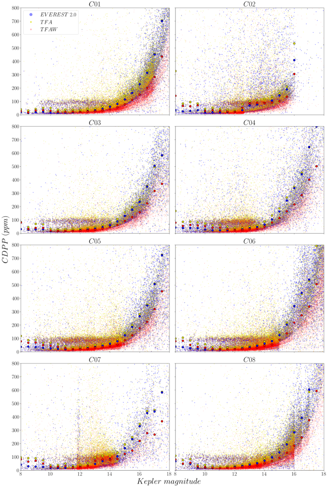
Figure 1: 6 hr CDPP as a function of $K_{p}$ for all K2 targets in campaigns C1-C8 corrected with EVEREST 2.0 (blue), TFA (yellow) and TFAW (red). The median in 0.5 magnitude-wide bins is indicated by blue circles for EVEREST 2.0, by yellow circles for TFA and red circles for TFAW.

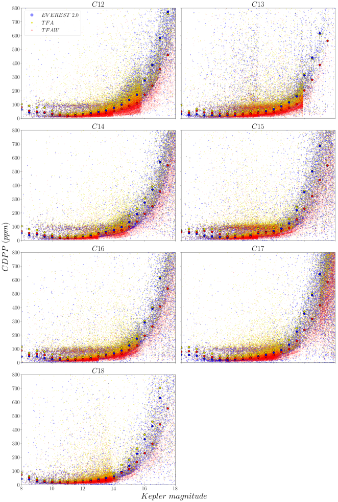
Figure 2: 6 hr CDPP as a function of $K_{p}$ for all K2 targets in campaigns C12-C18 corrected with EVEREST 2.0 (blue), TFA (yellow) and TFAW (red). The median in 0.5 magnitude-wide bins is indicated by blue circles for EVEREST 2.0, by yellow circles for TFA and red circles for TFAW.

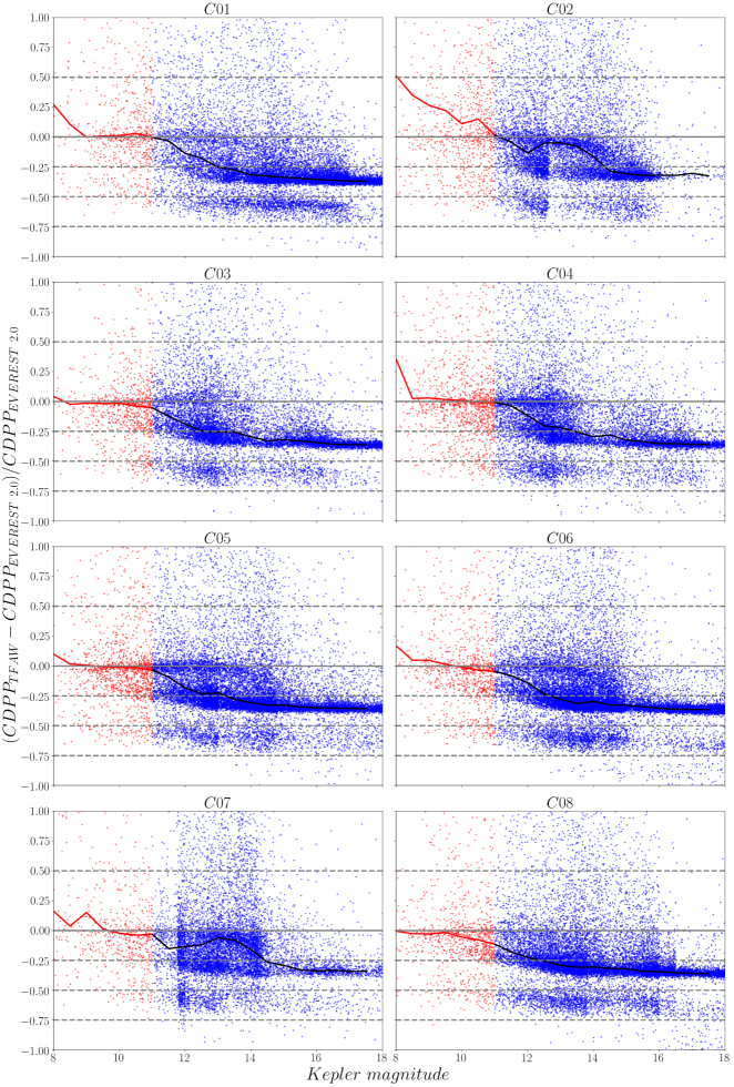
Figure 3: TFAW vs. EVEREST 2.0 relative 6 hr CDPP comparison for all K2 stars in campaigns C1 to C8. Individual stars are plotted as points, red for saturated stars ($K_{p}\lesssim$11 mag) and blue for fainter. Median relative 6 hr CDPP is plotted by a solid red line, for saturated stars ($K_{p}\lesssim$11 mag) and a solid black line for fainter magnitudes.

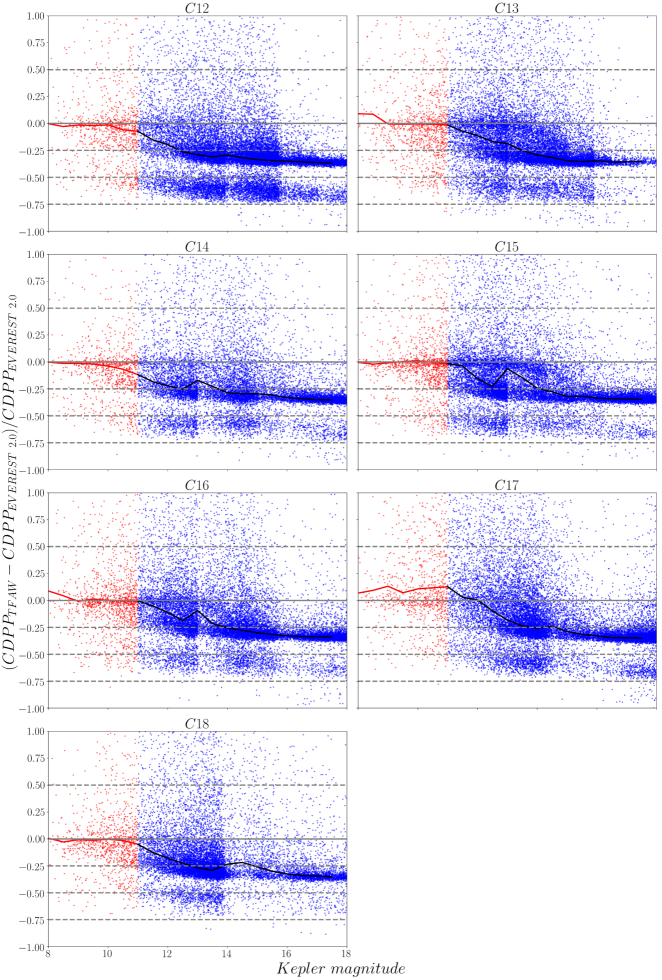
Figure 4: TFAW vs. EVEREST 2.0 relative 6 hr CDPP comparison for all K2 stars in campaigns C12 to C18. Individual stars are plotted as points, red for saturated stars ($K_{p}\lesssim$11 mag) and blue for fainter. Median relative 6 hr CDPP is plotted by a solid red line, for saturated stars ($K_{p}\lesssim$11 mag) and a solid black line for fainter magnitudes.

3.3 Transit detection efficiency

To assess the transit recovery rate we generate two sets of 5,000 randomly distributed test light curves covering magnitudes from $K_{p}$=8 to $K_{p}$=18, one simulating EVEREST 2.0 light curves and, the other, simulating light curves during TFAW’s frequency analysis step. The noise contribution for each of these light curves is estimated by fitting the EVEREST 2.0 and TFAW 6 hr CDDPs from Figures 1 and 2. After random white noise is injected, for each light curve at a given $K_{p}$ value, its corresponding CDPP value is randomly distributed, within a given width, around the fitted value.

To each of these light curves, we inject a transit signal selected from a random distribution of Sun-like (0.7-1.35$R_{\odot}$ and 0.8-1.5$M_{\odot}$) and Earth-like (0.5-2.3$R_{\oplus}$) systems with a random distribution of periods and transit epochs (ensuring at least two detectable transits), solar-like quadratic limb darkening coefficients, orbit inclinations and eccentricities.

We want to compare the transit detection rates obtained with EVEREST 2.0 and TFAW light curves using TLS. We use the following criteria to define a significant detection: firstly, the highest peak in the TLS power spectrum must have a period between $[\mathrm{P}_{\mathrm{s}}-0.01,\mathrm{P}_{\mathrm{s}}+0.01]$, where $\mathrm{P}_{\mathrm{s}}$ is the period of the simulated planetary transit, and secondly, the SDE_TLS of the highest peak in the power spectrum must be greater than 9.

We run TLS using the stellar limb darkening coefficients associated to each of the light curves and the transit search is done in the (0.01, 31.5) days range. We count the number of times the signal is detected in the TFAW light curves but not detected in the EVEREST 2.0 ones and the opposite test. Table 2 shows the number of non-simultaneous detections (both in absolute and percentage) for the 5,000 simulated Earth-Sun-like systems along the $K_{p}$ range for both EVEREST 2.0 and TFAW light curves. The number of non-simultaneous detections for the case of TFAW is a factor $\sim$8.5$\times$ higher than for the case of EVEREST 2.0 light curves. Also, the mean SDE_TLS values are higher for TFAW than for EVEREST 2.0. We also checked the false probability detection rate by seeing how many times the highest, non-aliased to the injected period peak in the power spectra crossed the threshold. We find similar results for EVEREST 2.0 and TFAW: 72 and 80 false detections, respectively.

Table 2: Mutually exclusive detections and mean SDE values for 5,000 simulated transits in Earth-Sun-like systems. $\mathrm{N}_{\mathrm{EVEREST}}$: not detected using TFAW light curves, but detected using EVEREST 2.0 data. $\mathrm{N}_{\mathrm{TFAW}}$: detected using TFAW light curves, but not detected using EVEREST 2.0 data. $\mathrm{N}_{\mathrm{mut}}$: simultaneous detections with EVEREST 2.0 and TFAW. $\mathrm{SDE}_{\mathrm{EVEREST}}$: mean EVEREST 2.0 SDE_TLS. $\mathrm{SDE}_{\mathrm{TFAW}}$: mean TFAW SDE_TLS. Percentage values in parenthesis are with respect to the 5,000 tested transits.

$\mathrm{N}_{\mathrm{EVEREST}}$	$\mathrm{N}_{\mathrm{TFAW}}$	$\mathrm{N}_{\mathrm{mut}}$	$\mathrm{SDE}_{\mathrm{EVEREST}}$	$\mathrm{SDE}_{\mathrm{TFAW}}$
80	681	2652	22.48	24.71
(1.6$\%$)	(13.6$\%$)	(53.1$\%$)

Table 3 shows the distribution of the EVEREST 2.0 and TFAW detections in three $K_{p}$ magnitude bins. In the bright-end regime TFAW shows 2.8$\times$ the number of detections of EVEREST 2.0. In the mid-$K_{p}$ range (11.0 $<K_{p}<$ 15.0), TFAW performs 8.9$\times$ better than EVEREST 2.0. Finally, in the faint-end case ($K_{p}>$15.0), TFAW detects the transit in 21.1$\times$ more light curves than EVEREST 2.0. This increase in the detection rate is in accordance with the improvement in the CDPP values for mid- and faint-magnitude range obtained with TFAW (see Figures 3 and 4).

Table 3: Detection distributions of ($\mathrm{N}_{\mathrm{EVEREST}}$, $\mathrm{N}_{\mathrm{TFAW}}$, $\mathrm{N}_{\mathrm{mut}}$) for the 5,000 simulated Earth-Sun-like systems as per three bins of $K_{p}$ magnitude.

$K_{p}<11.0$			$11.0<K_{p}<15.0$			$K_{p}>15.0$
$\mathrm{N}_{\mathrm{EVEREST2.0}}$	$\mathrm{N}_{\mathrm{TFAW}}$	$\mathrm{N}_{\mathrm{mut}}$	$\mathrm{N}_{\mathrm{EVEREST2.0}}$	$\mathrm{N}_{\mathrm{TFAW}}$	$\mathrm{N}_{\mathrm{mut}}$	$\mathrm{N}_{\mathrm{EVEREST2.0}}$	$\mathrm{N}_{\mathrm{TFAW}}$	$\mathrm{N}_{\mathrm{mut}}$
32	90	1290	36	338	1283	12	253	79

3.4 Transit injections

In del Ser et al. (2018) we show that, thanks to the wavelet approximation of the signal, TFAW is able to diminish the bias in the transit parameters. In order to ensure that TFAW returns an unbiased set of transit parameters, we run a transit injection/recovery test similar to the one used by Luger et al. (2016). We use a set of 2-day Savitsky-Golay filtered EVEREST 2.0 real K2 light curves with no known transit. We randomly select a sample of 3,400 stars from campaigns C1-C8 and C12-C18 with 8$\leq$$K_{p}$$\leq$18 magnitudes. Using the batman package (Kreidberg, 2015), the cataloged stellar properties (i.e. stellar mass and radius and quadratic limb darkening coefficients) for each target, assuming circular orbits, and randomly selecting the transit parameters (planetary radius to stellar radius ratio, orbital period, orbit inclination and transit epoch), we inject one planet (from a hot Jupiter to an Earth-sized planet) transit into each selected EVEREST 2.0 light curve. The injected transit depths range from $\sim 5\cdot 10^{-5}$ to $\sim 10^{-2}$. We then run TFAW to reconstruct and denoise the light curves. To determine whether the TFAW-corrected light curves can bias the transit depths, we fix all the parameters except for the planetary radius to stellar radius ratio, $p$, at their true values and recover the later. We fit the transit depth of the TFAW-corrected light curves by minimizing the residuals using the Levenberg-Marquardt method implemented in the lmfit package. Figure 5 shows the histogram of the recovered planetary radius to stellar radius ratio as a fraction of the injected one ($p/p_{0}$). As can be seen, the median $p/p_{0}$ for TFAW-reconstructed transits, is consistent with 1.0. We find an small <$\sim$2.5$\%$ bias towards smaller ratios for some of the transits. This bias starts to be significant for $p$<$\sim$0.011 (i.e transit depth smaller than $\sim 10^{-4}$). However, the relative difference between $p_{0}$ and the recovered planetary radius to stellar radius ratio is smaller than $\sim$0.0005 for almost all ($\sim$97$\%$) the simulated transits.

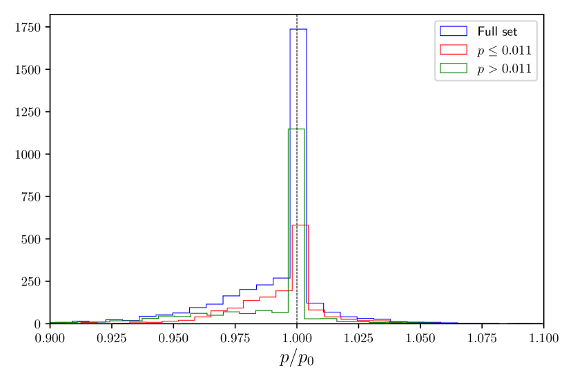
Figure 5: Histogram of transits with a certain planetary radius to stellar radius ratio as a fraction of the injected one ($p/p_{0}$) recovered after TFAW’s signal reconstruction step. Blue histogram corresponds to the 3,400 recovered transits; red histogram corresponds to those injected transits with $p\leq$0.011 and the green histogram corresponds to transits with $p$>0.011.

3.5 Characterization of known planets

In del Ser et al. (2018) we show that TFAW can improve the MCMC posterior distributions, diminish the bias in the fitted transit parameters and their uncertainties and narrow the credibility intervals for simulated transits. In this Section we compare EVEREST 2.0 and TFAW performance in terms of assessing the bias of the MCMC fitted transit parameters values and their uncertainties for two confirmed planetary systems with different SNRs: K2-44 b and K2-298 b.

3.5.1 Data description

As the starting point for the computation of TFAW, we use the PLD, CBV-corrected fluxes provided by the EVEREST 2.0 pipeline for both targets and all stars present in the same campaign and CCD module. 3072 epochs with the QUALITY=0 flag are considered and a 2-day Savitsky-Golay filter and a 5$\sigma$ outlier clipping are applied to the light curves. To iteratively denoise and reconstruct the light curves with TFAW, a template of reference stars for each target ($\sim$90) is built from a sub-set of stars from the same CCD module using Stetson’s L variability index (Stetson, 1996) to avoid the inclusion of bona-fide variable stars in the sample. We use this TFAW-corrected light curve to run the MCMC fit and compare it to the one obtained from the EVEREST 2.0 light curve.

Prior to the TFAW analysis, for both K2-44 b and K2-298 b we checked that the light curves we obtained directly from the EVEREST 2.0 matched with the ones after the transits have been masked. This way we ensure that any bias in the depth of the transiting planet is minimized (Luger et al., 2018).

3.5.2 Transit parameters fitting procedure

To characterize the target transits we use the analytic transiting model provided by the batman package with quadratic limb darkening coefficients as per Mandel & Agol (2002). We assume circular orbits (i.e. eccentricity=0) and fit the following five transit parameters: the transit epoch, $T_{0}$, the orbital period, $P$, the semi-major axis of the orbit, $a$, the planetary radius to stellar radius ratio, $p$, and the inclination of the orbit, $i$. We use the MCMC sampler provided by the emcee (Foreman-Mackey et al., 2013) package and use the george (Ambikasaran et al., 2015) package to create a combined model consisting on a Matérn 3/2 kernel plus a jitter or "white" noise term to generalize the likelihood function in order to consider covariances between data points (i.e correlated noise) and to minimize the bias of the inferred parameters. We consider a uniform distribution of the priors with wide enough bounds to let the chains explore the parameter space without getting close to the bound limit: $\pm 1$ day around the cataloged transit epoch for $T_{0}$, $\pm 3$ days for $P$, from 2$R_{*}$ to the cataloged semi-major axis plus 5$R_{*}$ for $a$, the cataloged planet/star ratio $\pm 0.01$ for $p$, and from 85^∘ to 90^∘ for $i$. We run the sampler with 100 walkers, 10,000 iterations with a burn-in phase of 2,000 iterations. This way we ensure that each of the chains run for more than 50 auto-correlation times for each parameter and that the mean acceptance fraction is between 0.25 and 0.5 (Bernardo et al., 1996; Foreman-Mackey et al., 2013).

3.5.3 K2-44: a confirmed high-SNR single planetary system example

K2-44 (EPIC 201295312) is a V=12.19$\pm$0.12 mag (Zacharias et al., 2012) located at $(\alpha,~{}\delta)$ = (11:36:02.79, -02:31:15.17) (Gaia Collaboration, 2018). It was observed by the K2 mission during the C1 monitoring campaign from May 30 to Aug 21, 2014. K2-44 was first reported as a planetary hosting candidate by Montet et al. (2015), and later validated, confirmed and characterized by Crossfield et al. (2016) and Mayo et al. (2018). For a more detailed summary of the stellar and planetary parameters see Table 4.

Table 4: Stellar and planetary parameters obtained for K2-44 b by Crossfield et al. (2016), Sing (2010), Mayo et al. (2018).

K2 ID	EPIC 201295312
Stellar parameters
Stellar radius $R_{\rm s}$ ($R_{\odot}$)	$1.58\pm 0.15$
Stellar mass $M_{\rm s}$ ($M_{\odot}$)	$1.150\pm 0.060$
Effective temperature (K)	$5912\pm 51$
Surface gravity ($log_{10}(cm/s^{2})$)	$4.101\pm 0.063$
Metallicity [Fe/H]	$0.0$ (assumed)
Spectral Type	-
Transit parameters
Period $P$ (days)	$5.65688\pm 0.00059$
Transit epoch $T_{0}$ (BJD - 2454833) (days)	$1978.7176\pm 0.0044$
Transit duration (hours)	$4.36\pm 0.13$
Eccentricity $e$	0 (assumed)
Radius ratio $p$	$0.0156\pm 0.0012$
$q_{1}$	$0.4752^{\dagger}$
$q_{2}$	$0.1914^{\dagger}$
Scaled semi-major axis $a$ (AU)	$0.0651\pm 0.0011$
Inclination $i$ (∘)	$87.354350^{+1.856108}_{-3.300347}$ ⋆
Planetary parameters
Planetary radius $R_{p}$ ($R_{\oplus}$)	$2.72\pm 0.32$
† denote values from Claret (2018) assuming 0.0 [Fe/H] metallicity.
⋆ denote values from Mayo et al. (2018).

To check whether the improved photometric precision yielded by TFAW in Section 3.2 results in a better characterization of the transiting signal we analyze EVEREST 2.0- and TFAW-corrected light curves for the confirmed exoplanet K2-44 b and compare the fitted parameters with the ones obtained by Crossfield et al. (2016) and Mayo et al. (2018). We assume a circular orbit ($e=0$), and a longitude of the periastron of $\omega$=90^∘. Using the stellar parameters provided by Crossfield et al. (2016) (see Table 4) and, assuming a metallicity of [Fe/H]=0.0, we fix the quadratic limb darkening coefficients to their theoretical values taken from Claret (2018).

In Table 5 we compare the transit parameters and their uncertainties obtained by Crossfield et al. (2016) and Mayo et al. (2018) with the ones obtained with EVEREST 2.0 and TFAW posterior probability distributions after running the MCMC fit as indicated in Section 3.5.2. The fitted parameter values are obtained from the 50% quantiles and their upper and lower errors are computed from the 25% and 75% quantiles, respectively.

Table 5: Top table: K2-44 b parameters from Crossfield et al. (2016), Mayo et al. (2018), and posterior transit parameters values and their uncertainties (25% and 75% quantiles) for EVEREST 2.0 and TFAW MCMC fits. Middle table: 95% confidence intervals of the highest probability density for K2-44 b transit parameters EVEREST 2.0 and TFAW MCMC fits. Bottom table: Derived parameters from Crossfield et al. (2016), Mayo et al. (2018), EVEREST 2.0, and TFAW.

MCMC Parameters	$T_{0}$ (BJD-2454833)	$P$ (days)	$a$ ($AU$)	$p$	$i$ (∘)
Crossfield et al. (2016)	1978.7176$\pm$0.0044	5.65688$\pm$0.00059	0.0651$\pm$0.0011	0.0156$\pm$0.0012	-
Mayo et al. (2018)	1978.72011${}^{+0.002565}_{-0.002557}$	5.656304${}^{+0.000366}_{-0.000323}$	-	0.017257${}^{+0.000704}_{-0.000538}$	87.354350${}^{+1.856108}_{-3.300347}$
EVEREST 2.0	1978.7248${}^{+0.0020}_{-0.0019}$	5.6549$\pm$0.0003	0.0644${}^{+0.0030}_{-0.0048}$	0.0149$\pm$0.0005	87.7663${}^{+1.1671}_{-1.3999}$
TFAW	1978.7094${}^{+0.0012}_{-0.0011}$	5.6570$\pm$0.0002	0.0600${}^{+0.0019}_{-0.0029}$	0.0141${}^{+0.0005}_{-0.0004}$	87.9933${}^{+1.0218}_{-1.1633}$
95% confidence intervals of the highest posterior density
EVEREST 2.0	1978.71873 - 1978.73143	5.65391 - 5.65598	0.05310 - 0.07049	0.01342 - 0.01645	84.96043 - 89.99988
TFAW	1978.70600 - 1978.71302	5.65638 - 5.65757	0.05308 - 0.06393	0.01302 - 0.01556	85.66826 - 89.99971
Derived system parameters		$R_{p}$ ($R_{\oplus}$)		b
Crossfield et al. (2016)		2.72$\pm$0.32		-
Mayo et al. (2018)		$2.93920584211^{+0.496465103254}_{-0.376603037856}$		-
EVEREST 2.0		$2.571^{+0.089}_{-0.089}$		$0.34^{+0.18}_{-0.21}$
TFAW		$2.433^{+0.089}_{-0.072}$		$0.29^{+0.15}_{-0.17}$

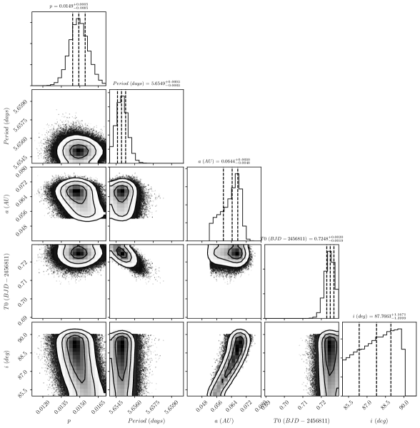
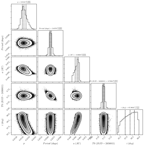
Figure 6: 1-D and 2-D projections of the posterior probability distributions of the 5 MCMC fitted parameters ($p$, $P$, $a$, $T_{0}$, $i$) for K2-44 b EVEREST 2.0 (top) and TFAW (bottom) light curves. The 25%, 50%, 75% quantiles, are displayed in dashed vertical lines on the 1-D histograms, and on the top each panels column.

The MCMC fit corner plot (Foreman-Mackey, 2016) for the K2-44 b transit is shown in Figure 6, yielding the following results: the time of inferior conjunction, $T_{0}$, for EVEREST 2.0 and TFAW are compatible with the one reported by Crossfield et al. (2016) and Mayo et al. (2018), though for TFAW, the uncertainties are much lower than for the other three ($\sim$2$\times$ for EVEREST 2.0, $\sim$2.5$\times$ for Mayo et al. (2018), and $\sim$4$\times$ compared to Crossfield et al. (2016)). For the semi-major axis of the orbit, $a$, EVEREST 2.0 and TFAW return smaller values than the one by Crossfield et al. (2016). However, while EVEREST 2.0 value is compatible within the errors with the one reported by Crossfield et al. (2016), this is not the case of TFAW. Though it is still compatible if ones takes into account the uncertainties in the stellar radius, impact parameter and orbit inclination. For the latter, both EVEREST 2.0 and TFAW yield values compatible with the reported value by Mayo et al. (2018). Again, TFAW returns the smallest uncertainties. Regarding the planetary to star radius ratio, $p$, both EVEREST 2.0 and TFAW obtain compatible values within the errors with the one reported by Crossfield et al. (2016). Again, TFAW returns the smallest uncertainties for this parameter and, compatible with the $p/p_{0}$ dispersion seen in Figure 5. For the period, $P$, the values from TFAW and EVEREST 2.0 are compatible with the cataloged ones. As for the previous parameters, TFAW returns the smallest uncertainties for the period. In summary, even for this rather high-SNR transit, TFAW returns lower uncertainties for all parameters compared with the EVEREST 2.0 and cataloged ones. Also, following the results in del Ser et al. (2018) with simulated transits, the transit parameters obtained with TFAW might be closer to the real ones (assuming that the planet orbits in a circular orbit). Finally, the widths of TFAW’s 95% confidence intervals are narrower for all parameters.

With the best fit parameters, EVEREST 2.0 obtains a mean planetary radius of $2.571^{\pm}0.089$ $R_{\oplus}$ and TFAW $2.433^{+0.089}_{-0.072}$ $R_{\oplus}$, both slightly below of the values reported by Crossfield et al. (2016) and Mayo et al. (2018), but compatible within the errors. Although $b$ is not reported either by Crossfield et al. (2016) or Mayo et al. (2018), we also derive it from the best fit parameters for EVEREST 2.0 to be $0.34^{+0.18}_{-0.21}$, and for TFAW to be $0.29^{+0.15}_{-0.17}$.

Figure 7 shows the summary plot displaying the PLD, CBV-corrected flux provided by the EVEREST 2.0 pipeline for K2-44 with the 2-day running median plotted in red, the EVEREST 2.0 median-filtered light curve and the TFAW-corrected light curves (with the MCMC derived transit data of the new candidate plotted in red), the TLS periodograms for EVEREST 2.0 and TFAW’s frequency analysis step; and the phase-folded light curves with the MCMC fit data (red line) for EVEREST 2.0 (left) and TFAW iteratively denoised and reconstructed one (right). The TLS periodograms show the position of the confirmed planet detected period (solid blue line) and its harmonics (dashed blue lines).

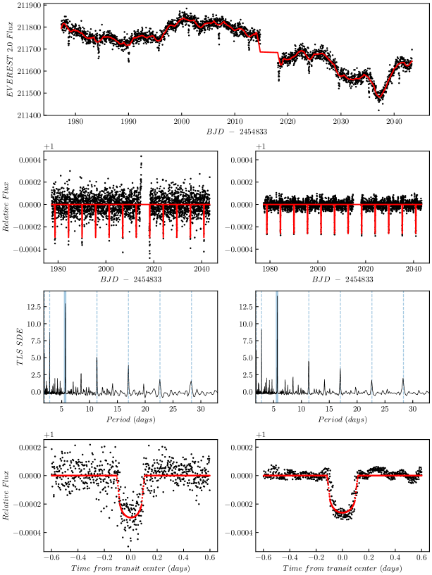
Figure 7: From top to bottom, the panels show the K2-44 raw flux of the EVEREST 2.0 light curve (with the running median in red), the entire light curve with in-transit data of the new candidate marked in red (left for EVEREST 2.0 and right for TFAW), the SDE_TLS periodogram (left for EVEREST 2.0 and right for TFAW), and the normalized phase-folded to the K2-44 b period light curve with MCMC fit data marked in red (left for EVEREST 2.0 and right for TFAW).

3.5.4 K2-298: a confirmed+candidate low-SNR multi planetary system example

K2-298 (EPIC201841433) is a V=14.87$\pm$0.01 mag (Zacharias et al., 2012) star located at $(\alpha,~{}\delta)$ = (11:40:49.62, +06:08:05.44) (Gaia Collaboration, 2018). It was observed by the K2 mission during the C1 monitoring campaign from May 30 to Aug 21, 2014. K2-298 was validated as a $0.802^{+0.081}_{-0.163}$ $M_{\odot}$ (Heller et al., 2019), $T_{eff}$=$5053^{+103}_{-166}$ K, $0.62846106^{+0.04341984}_{-0.02485835}$ $R_{\odot}$ (Gaia Collaboration, 2018) star orbited by an inner planet, K2-298 b, of $1.10^{+0.14}_{-0.12}$ $R_{\oplus}$ at $11.5^{+5.2}_{-2.6}$ $R_{\rm s}$ (Kruse et al., 2019) with a period of $4.16888^{+0.00050}_{-0.00056}$ days (Heller et al., 2019), and an outer candidate, EPIC201841433.01, of $2.11^{+0.23}_{-0.61}$ $R_{\oplus}$ at $29.5^{+14.7}_{-6.7}$ $R_{\rm s}$ with a period of $12.3389^{+0.0016}_{-0.0017}$ days (Kruse et al., 2019). Table 6 summarizes all the stellar and planetary parameters for K2-298 b.

As with the K2-44 case, we want to check whether the improved photometric precision yielded by TFAW results in a better characterization of the transiting signal. We analyze EVEREST 2.0- and TFAW-corrected light curves for the confirmed exoplanet K2-298 b and compare the fitted parameters with the ones obtained by Heller et al. (2019) and Kruse et al. (2019). We, again, assume a circular orbit ($e=0.0$), and a longitude of the periastron of $\omega$=90^∘. Using the stellar parameters in Table 6 and, assuming a metallicity of [Fe/H]=0.0, we fix the quadratic limb darkening coefficients to their theoretical values taken from Claret (2018).

Table 6: Stellar and planetary parameters obtained for K2-298 b by Heller et al. (2019), Kruse et al. (2019), Sing (2010), Gaia Collaboration (2018), Andrae et al. (2018).

K2 ID	EPIC 201841433
Stellar parameters
Stellar radius $R_{\rm s}$ ($R_{\odot}$)	$0.62846106^{+0.04341984}_{-0.02485835}$ ⋆⋆
Stellar mass $M_{\rm s}$ ($M_{\odot}$)	$0.802^{+0.081}_{-0.163}$
Effective temperature (K)	$5053^{+103}_{-166}$ ⋆⋆
Surface gravity ($log_{10}(cm/s^{2}$))	$4.595^{+0.050}_{-2.860}$
Metallicity [Fe/H]	$0.0$ (assumed)
Spectral Type	-
Transit parameters
Period $P$ (days)	4.16959${}^{+0.00051}_{-0.00053}$
Transit epoch $T_{0}$ (BJD - 2454833) (days)	2020.3300${}^{+0.0037}_{-0.0033}$
Transit duration (hours)	$2.400^{+0.264}_{-0.336}$ ⋆
Eccentricity $e$	0 (assumed)
Radius ratio $p$	0.0160${}^{+0.0017}_{-0.0016}$
$q_{1}$	$0.5510^{\dagger}$
$q_{2}$	$0.1575^{\dagger}$
Scaled semi-major axis $a$ (AU)	$0.0503^{+0.0227}_{-0.0114}$ ⋆
Inclination $i$ (∘)	$88.21$ ‡
Planetary parameters
Planetary radius $R_{p}$ ($R_{\oplus}$)	$1.10^{+0.14}_{-0.12}$
† denotes values from Claret (2018) assuming 0.0 [Fe/H] metallicity.
‡ denotes values derived assuming $b=0.36^{+0.24}_{-0.25}$ (Heller et al., 2019)
and $a$=$11.5^{+5.2}_{-2.6}~{}R_{\rm s}$ Kruse et al. (2019).
⋆ denotes values taken from Kruse et al. (2019).
⋆⋆ denotes values derived from Gaia Collaboration (2018)

In Table 7 we compare the transit parameters and their uncertainties obtained by Heller et al. (2019) and Kruse et al. (2019) with the ones obtained with EVEREST 2.0 and TFAW MCMC posterior probability distributions. As with K2-44 b, the fitted parameter values are obtained from the 50% quantiles and their upper and lower errors are computed from the 25% and 75% quantiles, respectively.

Table 7: Top table: K2-298 b parameters from Heller et al. (2019), Kruse et al. (2019), and posterior transit parameters values and their uncertainties (25% and 75% quantiles) for EVEREST 2.0 and TFAW MCMC fits. Middle table: 95% confidence intervals of the highest probability density for K2-298 b transit parameters EVEREST 2.0 and TFAW MCMC fits. Bottom table: Derived parameters from Heller et al. (2019), Kruse et al. (2019), EVEREST 2.0, and TFAW.

MCMC Parameters	$T_{0}$ (BJD-2454833)	$P$ (days)	$a$ ($AU$)	$p$	$i$ (∘)
Heller et al. (2019)	2020.3300${}^{+0.0037}_{-0.0033}$	4.16959${}^{+0.00051}_{-0.00053}$	-	0.0160${}^{+0.0017}_{-0.0016}$	-
Kruse et al. (2019)	1978.6338${}^{+0.0062}_{-0.0056}$	4.16888${}^{+0.00050}_{-0.00056}$	0.0503${}^{+0.0227}_{-0.0114}$	0.0205${}^{+0.0020}_{-0.0047}$	-
EVEREST 2.0	1978.6357${}^{+0.0024}_{-0.0023}$	4.1691${}^{+0.0003}_{-0.0003}$	0.0371${}^{+0.0026}_{-0.0020}$	0.0156${}^{+0.0007}_{-0.0007}$	88.8116${}^{+0.6143}_{-0.7022}$
TFAW	1978.6359${}^{+0.0011}_{-0.0012}$	4.1698${}^{+0.0001}_{-0.0001}$	0.0350${}^{+0.0009}_{-0.0010}$	0.0152${}^{+0.0004}_{-0.0003}$	89.0010${}^{+0.5117}_{-0.5574}$
95% confidence intervals of the highest posterior density
EVEREST 2.0	1978.62910 - 1978.64271	4.16828 - 4.16992	11.11698 - 15.22817	0.01355 - 0.01796	87.20658 - 89.99999
TFAW	1978.63245 - 1978.63912	4.16946 - 4.17010	11.11686 - 12.73192	0.01424 - 0.01641	87.84871 - 90.00000
Derived system parameters		$R_{p}$ ($R_{\oplus}$)		b
Heller et al. (2019)		1.10${}^{+0.14}_{-0.12}$		0.36${}^{+0.25}_{-0.24}$
Kruse et al. (2019)		1.41${}^{+0.15}_{-0.34}$		-
EVEREST 2.0		1.072${}^{+0.061}_{-0.054}$		0.26${}^{+0.14}_{-0.16}$
TFAW		1.040${}^{+0.037}_{-0.032}$		0.21${}^{+0.11}_{-0.12}$

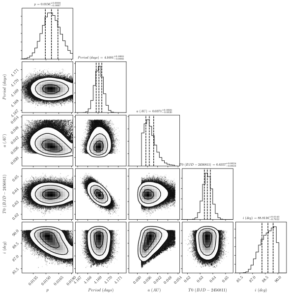
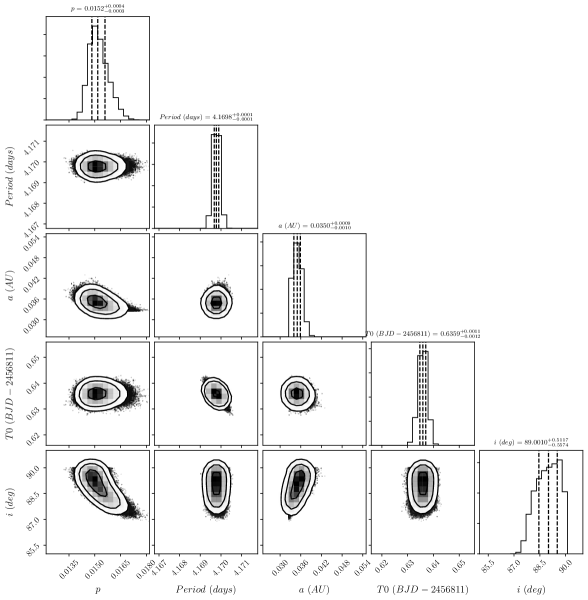
Figure 8: 1-D and 2-D projections of the posterior probability distributions of the 5 MCMC fitted parameters ($p$, $P$, $a$, $T_{0}$, $i$) for K2-298 b EVEREST 2.0 (top) and TFAW (bottom) detrended light curves. The 25%, 50%, 75% quantiles, are displayed in dashed vertical lines on the 1-D histograms and on the top each panels column.

For the best fit (shown in Figure 8), the mid-transit, $T_{0}$, for EVEREST 2.0 and TFAW is compatible with the one reported by Kruse et al. (2019), though for TFAW, the uncertainties are much lower than for the other two ($\sim$2$\times$ for EVEREST 2.0, and $\sim$5$\times$ compared to Kruse et al. (2019)). The value given by Heller et al. (2019) corresponds to the first transit after the center of the respective K2 target light curve. For the orbit inclination, $i$, neither Heller et al. (2019) nor Kruse et al. (2019) report a value. However, both EVEREST 2.0 and TFAW yield values which are compatible within their errors and as with the previous parameters, TFAW returns the smallest uncertainties ($\sim$1.2$\times$ compared to EVEREST 2.0). For the period, $P$, the values found for EVEREST 2.0 and TFAW are compatible within the errors with the one in Heller et al. (2019) and are very close to the one in Kruse et al. (2019). Again, TFAW returns the smallest uncertainties for this parameter ($\sim$3$\times$ for EVEREST 2.0, $\sim$5$\times$ for Heller et al. (2019) and Kruse et al. (2019)). For the semi-major axis of the orbit, $a$, EVEREST 2.0 and TFAW values are compatible taking the lower errors with the one reported by Kruse et al. (2019). Again, TFAW returns the smallest uncertainties for this parameter ($\sim$2$\times$ for EVEREST 2.0, and $\sim$10$\times$ compared to Kruse et al. (2019)). Finally, regarding the planetary to star radius ratio, $p$, both EVEREST 2.0 and TFAW obtain compatible values within the errors with the one reported by Heller et al. (2019). With respect the value reported by Kruse et al. (2019), it is compatible taking into account the reported planetary and stellar radius uncertainties. As with the other parameters, TFAW returns the smallest uncertainties for this parameter ($\sim$2$\times$ for EVEREST 2.0, $\sim$7$\times$ for Kruse et al. (2019), and $\sim$5$\times$ compared to Heller et al. (2019)) and again, compatible with the $p/p_{0}$ dispersion seen in Figure 5. As with K2-44 b, the widths of TFAW’s 95% confidence intervals are narrower for all parameters.

With the best fit parameters, EVEREST 2.0 obtains a mean planetary radius of $1.072^{+0.061}_{-0.054}$ $R_{\oplus}$ and TFAW $1.040^{+0.037}_{-0.032}$ $R_{\oplus}$, compatible with the $1.10^{+0.14}_{-0.12}$ $R_{\oplus}$ reported by Heller et al. (2019) and $1.41^{+0.15}_{-0.34}$ $R_{\oplus}$ reported by Kruse et al. (2019). We also derive $b$ from the best fit parameters, for EVEREST 2.0 to be $0.26^{+0.14}_{-0.16}$, and for TFAW to be $0.21^{+0.11}_{-0.12}$, both compatible with the one in Heller et al. (2019). For both derived parameters, TFAW returns the lowest uncertainties.

Figure 9 shows the summary plot displaying the PLD, CBV-corrected flux provided by the EVEREST 2.0 pipeline for K2-298 with the 2-day running median plotted in red, the EVEREST 2.0 median-filtered light curve and the TFAW-corrected light curves (with the MCMC derived transit data of the new candidate plotted in red), the TLS periodograms for EVEREST 2.0 and TFAW’s frequency analysis step; and the phase-folded light curves with the MCMC fit data (red line) for EVEREST 2.0 (left) and TFAW iteratively denoised and reconstructed one (right). The TLS periodograms show the position of the candidate planet detected period (Kruse et al., 2019) (solid blue line) and its harmonics (dashed blue lines) and the position of K2-298 b period (solid red line).

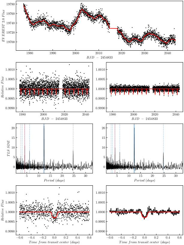
Figure 9: From top to bottom, the panels show the K2-298 raw flux of the EVEREST 2.0 light curve (with the running median in red), the entire light curve with in-transit data of the new candidate marked in red (left for EVEREST 2.0 and right for TFAW), the SDE_TLS periodogram (left for EVEREST 2.0 and right for TFAW), and the normalized phase-folded to the K2-298 b period light curve with MCMC fit data marked in red (left for EVEREST 2.0 and right for TFAW).

3.5.5 TFAW’s limitations

The small oscillations in some of the TFAW detrended and denoised light curves, such as in the lower right panel of Figure 7, might be explained by one of or a combination of the following three factors. First, real correlated noise in the decomposition levels above the chosen signal level that may have not been properly removed during the TFAW detrending stage. Second, in some cases, real stellar variability with different time scales can be present at the same decomposition levels associated with the phased folded transit signal. As a consequence, this stellar variability can be included in the signal estimation, reconstruction and denoising process. Third, spurious features in the signal estimation arising from the shape of the mother wavelet or an alias due to the sampling of the data in the phase folded light curve. These two later effects cannot be fully discarded but the signal estimation can be improved by increasing the number of decomposition levels or by optimizing the signal level selection criteria. On the other hand, signals caused by stellar activity or pulsation are unique to each star and temporally correlated, and can not be easily removed by decorrelation or denoising techniques. For example, the bump around phase [+0.2,+0.3] seen in the K2-44 b TFAW phase-folded light curve at the lower right panel of Figure 7, is also present in the EVEREST 2.0 at the same phase interval. The removal of temporally correlated noise can be difficult to do using the SWT. Although this is beyond the scope of this paper, future versions of the TFAW can benefit from: the incorporation of GP to model the covariance structure of the correlated noise (Chakrabarty & Sengupta, 2019), modeling of the signal of interest in the wavelet domain (Goossens et al., 2009) or thresholding the wavelet coefficients (Jansen & Bultheel, 1999) prior to the Inverse Stationary Wavelet Transform (ISWT) at each level to reduce the correlated noise. Another way to diminish the effects of correlated noise (which has a higher frequency in the phase folded light curve than the transit signal) would be to increase the noise level or to increase the number of decomposition levels (i.e. adding more epochs to the light curve) as to better separate the different signal contributions at different frequencies. The later is not possible with K2 data as the number of available epochs in the archive is fixed. It is worth mentioning that we have been extremely careful when selecting the noise and signal levels to minimize the chances of removing part of the signal of interest contribution, so the results could improve by a more aggressive selection of those levels.

4 Testing transit search with TFAW: two transit candidates in K2 observing campaign C1

In this Section we present partial results obtained after the application of TFAW to EVEREST 2.0 light curves from the K2 observing campaign C1. We present two new Earth-sized transiting planet candidates detected using TLS during TFAW’s frequency analysis step (i.e. light curve is detrended and has had a first SWT noise estimation removed). For both cases we show their transit parameters obtained with MCMC after TFAW’s iterative signal denosing and reconstruction. A more extensive planet search, not only for C1 but for all K2 campaigns, and using fully automatic vetting (Kostov et al., 2019; Zink et al., 2020) is underway. With this study, which is to be completed soon for an upcoming publication, we will obtain more potential new candidates.

In this Section we also compare our ability to recover confirmed and candidate transit planets detected by other searches for C1.

4.1 Data description

We use the PLD, CBV-corrected fluxes provided by the EVEREST 2.0 pipeline for K2 observing campaign C1. For each light curve, 3072 epochs with the QUALITY=0 flag are considered. Given that the goal is to search for transiting signals, a 2-day Savitsky-Golay filter is applied to remove or minimize the effects of stellar variability. After the filter has been applied, light curves have their outliers removed using a 5$\sigma$ clipping. An extra outlier removal is done by TFAW prior to the period search using a wavelet estimation of the signal (see del Ser et al. (2018) for more details). To iteratively denoise and reconstruct the light curves with TFAW, a template of reference stars for each light curve ($\sim$90) is built from a sub-set of stars from the same CCD module. To avoid the inclusion of variable stars in this template, we use Stetson’s L variability index (Stetson, 1996).

4.2 Transit search and vetting criteria

We follow a transit search, vetting, and False-Positive Probability (FPP) approach similar to the one detailed in Heller et al. (2019). First, we use TLS to search for transiting signals during TFAW’s frequency analysis step. TLS is run using modelled stellar parameters, $M_{\rm s}$ , $R_{\rm s}$ , $u_{\rm 1}$ , and $u_{\rm 2}$ . All light curves that have a TLS power spectrum peak with an SDE_TLS greater than 9 (false-positive rate $<$10^-4 (Hippke & Heller, 2019)) are considered a significant detection and undergo TFAW’s iterative signal reconstruction and denoising. Then, we visually inspect those TFAW-corrected light curves and only keep the ones which visually show transit-like features.

Following the same procedure as Heller et al. (2019), all transits are required to have at least 0.5 days from the beginning or end of any gaps in their light curves to avoid false positives. If a candidate had three or fewer transits, they should have a SNR$>$10. In addition, to reject eclipsing binaries, for all candidates the average depth of the odd and even transits should agree within $<$3$\sigma$ and objects should not present evidence of a secondary eclipse at the $>$3$\sigma$ level at half an orbital phase after the candidate transit.

For those light curves we consider of interest, we include some extra vetting steps with respect to the procedure in Heller et al. (2019) to increase the reliability of the candidates. First, we perform an extensive bibliographic search of such target. We cross-match this source with the most up-to-date (8 Mar 2020 for this work) K2-C1 lists of confirmed or candidate exoplanets from the NASA Exoplanet Archive (Akeson et al., 2013) or in the Vizier database. We also check if the target shows any known kind of variability or pulsation (Armstrong et al., 2015, 2016; Watson et al., 2006). The updated stellar parameters and the 2MASS and SDSS photometry of the host stars are retrieved from catalogs such as EPIC (Huber et al., 2016), Gaia-DR2 (Gaia Collaboration, 2018) and Claret (2018). We also search if the candidates have been observed by the TESS mission (Ricker et al., 2015). Second, we rule out that no other light curve in the same CCD module present transit-like features with similar periods and transit epochs as the candidate. Third, we compare the TLS and BLS (Kovács et al., 2002) periodograms to check if they present similar peaks. Next, to diminish the chances of the TLS detection being fortuitous, we randomly reshuffle the target light curve to remove the transiting signal and to simulate 1,000 light curves with similar CDPP as the TFAW’s frequency analysis step light curve. Using the batman package, we inject a transit signal with the parameters found by TLS. We run TLS over the simulated light curves and check whether the transit is recovered or not. If the transit is recovered in more than 90% of the simulated light curves, then it passes to the final vetting step. We use the publicly available vespa software (Morton, 2012, 2015) to evaluate the FPP of our transit candidates. For each of the candidates, we supply the software with their corresponding TFAW phase folded light curve, their celestial coordinates, the stellar parameters of their host star, and its photometry. We also compute a limiting aperture obtained from the validation sheets from the EVEREST 2.0 database, and inspect independent photometry and high angular resolution images to evaluate contamination from other sources. Using such information, vespa calculates the probabilities of the transiting signal being caused by non-associated blended eclipsing binaries, eclipsing binaries, hierarchical triples and non-associated stars with transiting planets. Only candidates with a FPP lower than 1% are considered as valid candidates.

4.3 Comparison with other searches

In Table 8 we show that our K2-C1 TFAW and TLS based planet search is able to recover all confirmed planets and most of the K2 candidates from previous studies compiled in NASA Exoplanet Archive. Generally, the missing ones are usually single-transit events, not suitable for periodic signal searching algorithms like TLS, multi-periodic systems for which the current TFAW version only reconstructs the signal for the most significant period (though the other planets in the system might have also been detected in the TLS periodogram but with lower SDEs), or some that present an SDE${}_{\rm TLS}<$9 (usually above 6.5) but have their most significant peak at the catalogued period. For the confirmed planets, TFAW finds at least one planet for each of the 35 cataloged planetary systems. For the ones in Barros et al. (2016), TFAW detects 18 transiting systems, one, with a period $>$40 days is missed by TLS, and for another TLS does not find a significant peak at the listed period. For Crossfield et al. (2016), we detect 9 of the 13 listed candidates for C1. Two of the missing ones are candidates with periods $>$40 days; for the other two TLS does not find a significant peak at the listed periods. Regarding Vanderburg et al. (2016), we detect 68 of the listed candidates. The other four are single-transit or have a period $>$40 days. We detect all the candidates for C1 listed by Mayo et al. (2018). Finally, we detect at least one planet in all 78 non-single-transit systems in Kruse et al. (2019). We believe our new candidates presented here went undetected by other groups due to the combination of two factors, the increased photometric precision achieved with TFAW, specially for faint magnitudes, together with TLS improved capabilities to detect smaller planets.

Table 8: Comparison of our planet search to previous groups, all sub-sampled to K2-C1 campaign.

Candidate List	Cataloged planets	Number we found
Confirmed	48	35
Barros et al. (2016)	20	18
Crossfield et al. (2016)	13	9
Vanderburg et al. (2016)	72	68
Mayo et al. (2018)	13	13
Kruse et al. (2019)	97	78

4.4 Two new transit candidates from K2-C1 data

In this Section we present two new transit candidates detected using the combination of the increased photometric precision of TFAW-corrected light curves and TLS. Both candidates have passed the vetting procedure explained in 4.2. As with K2-44 b and K2-298 b, once detected, we checked the EVEREST 2.0 light curves after masking the new candidate transits (given their smaller transit depths, the effect of the PLD can decrease the transit depth up to $\sim$10% (Luger et al., 2018)). Finally, in order to determine the transit parameters of these new candidates, we use the TFAW-corrected light curves, the TLS output and the cataloged stellar properties as the starting point for the MCMC fit. As mentioned before, a complete study of observing campaign C1 (and C2-C18) is underway where more transit candidates are expected to be found. In Tables 9 and 10 we summarize the stellar and transit properties of the two new planetary candidates fully described in Sections 4.4.1 and 4.4.2.

4.4.1 EPIC 201170410

EPIC 201170410 is a $K_{p}$=15.673 mag, $G$=16.4386 mag (Gaia Collaboration, 2018), $K_{s}$=12.619$\pm$0.027 mag, $(J-K_{s})$=0.84$\pm$0.037 (Cutri et al., 2003) star. It is located at $(\alpha,~{}\delta)$ = (11:20:33.81, -04:48:25.21) (Gaia Collaboration, 2018) and observed by the K2 mission during the C1 monitoring campaign, channel 55.

Table 9 lists the cataloged stellar parameters by Huber et al. (2016) and Stassun et al. (2019) for this source. Gaia Collaboration (2018) provides a $T_{eff}$=$4013^{+714}_{-713}$ K, which is compatible within the previous listed value. This target is classified as a dwarf by Stassun et al. (2019) and, given its cataloged radius, mass and effective temperature it is most likely an M-dwarf. No variability detection for this star is provided either in Armstrong et al. (2015, 2016), Watson et al. (2006) or Gaia Collaboration (2018).

Table 9: Stellar parameters for EPIC 201170410 host star, TLS-detection parameters for the transit planetary candidate EPIC 201170410.02, TLS and vespa vetting parameters, and MCMC fit and derived planetary candidate parameters of EPIC 201170410.02.

K2 ID	EPIC 201170410
Stellar parameters
Stellar radius $R_{\rm s}$ ($R_{\odot}$)	$0.282^{+0.074}_{-0.069}$ ⋆
Stellar mass $M_{\rm s}$ ($M_{\odot}$)	$0.287^{+0.101}_{-0.084}$ ⋆
Effective temperature (K)	$3648^{+172}_{-143}$ ⋆
Surface gravity ($log_{10}(cm/s^{2}$))	4.999$\pm$0.075 ⋆
Metallicity [Fe/H]	$-0.048^{+0.150}_{-0.210}$ ⋆
Distance (pc)	$134.0^{+45.8}_{-39.8}$ ⋆
Luminosity $L_{\rm s}$ ($L_{\odot}$)	-
Luminosity class	Dwarf ⋆⋆
Spectral Type	-
TLS-detection transit parameters
Number of transits	10 †
Period $P$ (days)	6.799025
Epoch $T_{0}$ (BJD - 2454833) (days)	1980.14697625
Duration (hours)	1.84933104
Depth $\delta$ (%)	0.136
SNR	6.97 ††
Radius ratio $p$	0.0335913
Scaled semi-major axis $a$ (AU)	0.0463297
Planetary radius $R_{p}$ ($R_{\oplus}$)	1.0332548
TLS and vespa vetting parameters
SDETLS	9.382
$\rho\,($″$)$	22.5
FPP	$4.8~{}\times~{}10^{-10}$
MCMC transit parameters
Period $P$ (days)	6.7987$\pm$0.0001
Epoch $T_{0}$ (BJD - 2454833) (days)	1980.1485${}^{+0.0006}_{-0.0005}$
Eccentricity $e$	0 (assumed)
Radius ratio $p$	0.0340${}^{+0.0007}_{-0.0006}$
Scaled semi-major axis $a$ (AU)	$0.0349^{+0.0027}_{-0.0022}$
Inclination $i$ (∘)	$89.0025^{+0.4142}_{-0.2885}$
Derived planetary parameters
Planetary radius $R_{p}$ ($R_{\oplus}$)	$1.047^{+0.276}_{-0.257}$ ‡
Impact parameter $b$	$0.46^{+0.20}_{-0.14}$ ‡
† denotes number of transits detected by TLS that have data.
‡ denotes values derived from fitted values.
†† as defined in Pont et al. (2006).
⋆ denotes values derived from Huber et al. (2016).
⋆⋆ denotes values derived from Stassun et al. (2019).

Table 9 also summarizes the detection and vetting parameters obtained with TLS and vespa for the EPIC 201170410 TFAW-corrected light curve. With an SDE_TLS>9.0 and an FPP of $4.8~{}\times~{}10^{-10}$ it can be considered an statistically validated exoplanet candidate (Heller et al., 2019). Finally, it also lists the transit and derived planetary parameters obtained from the MCMC fit of the TFAW-corrected light curve.

Figure 10 shows the summary plot displaying the PLD, CBV-corrected flux provided by the EVEREST 2.0 pipeline for EPIC 201170410 with the 2-day running median plotted in red, the EVEREST 2.0 median-filtered light curve and the TFAW-corrected light curves (with the MCMC derived transit data of the new candidate plotted in red), the TLS periodograms for EVEREST 2.0 and TFAW’s frequency analysis step; and the phase-folded lights curve with the MCMC fit data (red line) for EVEREST 2.0 (left) and TFAW iteratively denoised and reconstructed one (right). The TLS periodograms show the position of the candidate’s detected period (solid blue line) and its harmonics (dashed blue lines).

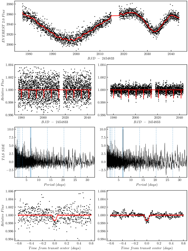
Figure 10: From top to bottom, the panels show the EPIC 201170410 raw flux of the EVEREST 2.0 light curve (with the running median in red), the entire light curve with in-transit data of the new candidate marked in red (left for EVEREST 2.0 and right for TFAW), the SDE_TLS periodogram (left for EVEREST 2.0 and right for TFAW), and the normalized phase-folded light curve with MCMC fit data marked in red (left for EVEREST 2.0 and right for TFAW).

As can be seen from the TLS periodograms, the peak at 6.7987 days is visible both for EVEREST 2.0 and TFAW. However, for the latter, and given TFAW’s denoising capabilities, this peak has a higher SDE_TLS (9.4 versus 7.4) that allows it to cross our significant detection threshold (i.e $>$9). In the particular case of EVEREST 2.0 detrended light curve, EPIC 201170410.02 might not have been detected by other authors, even those using TLS, because the light curve noise sets the SDE_TLS below the detection threshold employed by them (9.0 in the case of Hippke & Heller (2019) and Heller et al. (2019)). In addition, the transit-like feature becomes clearly visible in the reconstructed TFAW light curve (right plot in the second row in Figure 10 and right bottom plot in Figure 10). It is worth mentioning that the wavelet does not have an a priori knowledge of the shape of the underlying signal in a given light curve and that its shape is estimated only from the phase folded light curve at a given period and is re-estimated at every iteration step during TFAW’s signal reconstruction step. As show in Section 3.5.4 with K2-298 b, EPIC 201170410 shows another example of the potential of TFAW to detect and recover transit-like features even for highly noisy light curves as this one.

To confirm that our candidate light curve was not affected by contamination of nearby sources, we visually inspect the K2-C1, channel 55, calibrated full frame images (FFI) for EPIC 201170410. In addition, Gaia Collaboration (2018) does not list any other source within EPIC 201170410 aperture either. As explained in Section 4.2, using EVEREST 2.0 validation sheets for EPIC 201170410 we assigned the maximum aperture radius for vespa, $\rho\,$=22.5$\arcsec$, to estimate the possibility of contamination by other objects.

EPIC 201170410 has also been observed by the TESS mission in Sector 9 (28 Feb to 26 Mar 2019). EPIC 201170410 corresponds to TIC 38116202. However, no light curve for this target is available from the usual TESS data archives. We download the TESS FFI corresponding to TIC 38116202 using the eleanor package and use it to compute raw, CBV-corrected and PSF-modeled light curves for this target. TIC 38116202 is highly affected by crowding from two other near and brighter stars in the TESS FFI leading to a worse photometric solution than the one from K2 thus, no conclusive results can be obtained from this light curve after running the period search using TLS.

Finally, in order to better determine the EPIC 201170410.02 transit and planetary parameters, we run a MCMC fit over the TFAW-corrected light curve using the TLS output as initial guess values. Table 9 lists the obtained MCMC fit and planetary derived values. For EPIC 201170410.02 and, assuming a circular orbit, TFAW yields a 1.047${}^{+0.276}_{-0.257}R_{\oplus}$ planet orbiting its host star at 0.0349${}^{+0.0027}_{-0.0022}$ AU with a period of 6.7987$\pm 0.0001$ days. With this radius value, EPIC 201170410.02 is the 10-th smallest K2-C1 planet within those candidates with an estimated planetary radius and the 44-th smallest in all K2 campaigns.

4.4.2 EPIC 201757695

EPIC 201757695 is a $K_{p}$=14.599 mag, $G$=14.6206 mag (Gaia Collaboration, 2018), $K_{s}$=12.149$\pm$0.026 mag, $(J-K_{s})$=0.707$\pm$0.037 (Cutri et al., 2003) star. It is located at $(\alpha,~{}\delta)$ = (11:35:45.24, +04:36:59.21) (Gaia Collaboration, 2018) and observed by the K2 mission during the C1 monitoring campaign, channel 47.

Table 10 lists the cataloged stellar parameters by Huber et al. (2016), Bailer-Jones et al. (2018), Gaia Collaboration (2018) and Stassun et al. (2019) for this source. In addition, Gaia Collaboration (2018) provides a $T_{eff}$=$4706^{+290}_{-264}$ K, which is compatible within the previous listed value. This star is classified as a dwarf (Stassun et al., 2019) and, given its cataloged radius, mass and effective temperature it is most likely a K-type star. No variability detection for this star is provided either in Armstrong et al. (2015, 2016) or Gaia Collaboration (2018). It is cataloged as a "variable star of unspecified type" (VAR) by the AAVSO International Variable Star Index (VSX) (Watson et al., 2006) with a period of 19.94041 days.

Table 10: Stellar parameters for EPIC201757695 host star, TLS-detection parameters for the transit planetary candidate EPIC201757695.02, TLS and vespa vetting parameters, and MCMC fit and derived planetary candidate parameters of EPIC201757695.02.

K2 ID	EPIC 201757695
Stellar parameters
Stellar radius $R_{\rm s}$ ($R_{\odot}$)	$0.655^{+0.041}_{-0.045}$ ⋆
Stellar mass $M_{\rm s}$ ($M_{\odot}$)	$0.727^{+0.044}_{-0.053}$ ⋆
Effective temperature (K)	$4520^{+108}_{-54}$ ⋆
Surface gravity ($log_{10}(cm/s^{2}$))	$4.659^{+0.035}_{-0.025}$ ⋆
Metallicity [Fe/H]	$-0.003^{+0.120}_{-0.300}$ ⋆
Distance (pc)	$577.6^{+33.2}_{-29.8}$ ⋆⋆
Luminosity $L_{\rm s}$ ($L_{\odot}$)	$0.433^{+0.482}_{-0.385}$ ⋆⋆⋆
Luminosity class	Dwarf ⋆⋆⋆⋆
Spectral Type	-
TLS-detection transit parameters
Number of transits	30 †
Period $P$ (days)	2.04779036
Epoch $T_{0}$ (BJD - 2454833) (days)	1978.6419269
Duration (hours)	1.82256
Depth $\delta$ (%)	0.021
SNR	11.04 ††
Radius ratio $p$	0.01248
Scaled semi-major axis $a$ (AU)	0.0283772
Planetary radius $R_{p}$ ($R_{\oplus}$)	0.891695
TLS and vespa vetting parameters
SDETLS	15.005
$\rho\,($″$)$	18.3
FPP	$8.13~{}\times~{}10^{-5}$
MCMC transit parameters
Period $P$ (days)	2.0478$\pm$0.0001
Epoch $T_{0}$ (BJD - 2454833) (days)	1978.6370${}^{+0.0008}_{-0.0007}$
Eccentricity $e$	0 (assumed)
Radius ratio $p$	0.0127$\pm$0.0002
Scaled semi-major axis $a$ (AU)	0.0296$\pm$0.0005
Inclination $i$ (∘)	$89.2757^{+0.3689}_{-0.3717}$
Derived planetary parameters
Planetary radius $R_{p}$ ($R_{\oplus}$)	$0.90819^{+0.05861}_{-0.06401}$ ‡
Impact parameter $b$	0.12$\pm$0.06 ‡
† denotes number of transits detected by TLS that have data.
‡ denotes values derived from fitted values.
†† as defined in Pont et al. (2006).
⋆ denotes values derived from Huber et al. (2016).
⋆⋆ denotes values derived from Bailer-Jones et al. (2018).
⋆⋆⋆ denotes values derived from Gaia Collaboration (2018).
⋆⋆⋆⋆ denotes values derived from Stassun et al. (2019).

Table 10 also lists the detection and vetting parameters obtained with the TLS and vespa for the EPIC 201757695 TFAW-corrected light curve. With an SDE${}_{\rm TLS}>$9 and an FPP of 8.13$\times 10^{-5}$ EPIC 201757695.02 can be considered an statistically validated exoplanet candidate. Finally, Table 10 also summarizes the transit and derived planetary parameters obtained from the MCMC fit of the TFAW-corrected light curve.

Figure 11 shows the summary plot displaying the PLD, CBV-corrected flux provided by the EVEREST 2.0 pipeline for EPIC 201757695 with the 2-day running median plotted in red, the EVEREST 2.0 median-filtered light curve and the TFAW-corrected light curves (with the MCMC derived transit data of the new candidate plotted in red), the TLS periodograms for EVEREST 2.0 and TFAW’s frequency analysis step; and the phase-folded light curves with the MCMC fit data (red line) for EVEREST 2.0 (left) and TFAW iteratively denoised and reconstructed one (right). The TLS periodograms show the position of the candidate’s detected period (solid blue line) and its harmonics (dashed blue lines).

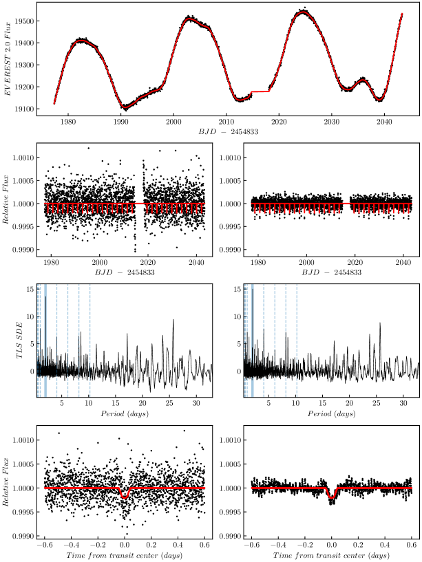
Figure 11: From top to bottom, the panels show the EPIC 201757695 raw flux of the EVEREST 2.0 light curve (with the running median in red), the entire light curve with in-transit data of the new candidate marked in red (left for EVEREST 2.0 and right for TFAW), the SDE_TLS periodogram (left for EVEREST 2.0 and right for TFAW), and the normalized phase-folded light curve with MCMC fit data marked in red (left for EVEREST 2.0 and right for TFAW).

The TLS periodograms in Figure 11 show a clear peak at 2.048 days and with enough SDE_TLS to cross our detection threshold both for EVEREST 2.0 and TFAW. However, for the latter, again due to TFAW denoising capabilities, this significance is higher (15.0 versus 14.2). As with the case of EPIC 201170410, for EPIC 201757695 the transit feature becomes clearly more visible in the TFAW-corrected light curve.

To confirm that this second candidate was not affected by contamination from nearby sources, we visually inspect the K2 calibrated full frame images (FFI) for EPIC 201757695. In addition, Gaia Collaboration (2018) does not show any other source within EPIC 201757695 aperture. Using EVEREST 2.0 validation sheets for this target, we assigned the maximum aperture radius for vespa, $\rho\,$=18.3$\arcsec$ as listed in Table 10.

EPIC 201757695 is included in the TESS Input Catalog (Stassun et al., 2019) as TIC 903075188. However, to date 31 Mar 2020, it has not been observed yet and no light curve is available for this target.

Again, in order to better determine EPIC 201757695.02 transit and planetary parameters, we run a MCMC fit over this target TFAW-corrected light curve using the TLS output as initial guess values.

Table 10 lists the obtained MCMC fit and planetary derived values. For EPIC 201757695.02 and, assuming a circular orbit, TFAW yields a 0.908${}^{+0.059}_{-0.064}R_{\oplus}$ planet orbiting its host star at a distance of 0.0296$\pm 0.0005$ AU with a period of 2.0478$\pm 0.0001$ days. With this radius value, EPIC 201757695.02 is the 9-th smallest K2-C1 of the candidates with an estimated planetary radius, and the 39-th smallest in all K2 campaigns.

5 Conclusions

We present the results obtained after applying the wavelet-based TFAW to further extend the photometric precision achieved by EVEREST 2.0 light curves from the K2 mission. We compare the photometric precision of both algorithms in terms of the 6hr CDPP. On average, the TFAW median 6hr CDPP is $\sim$30$\%$ better than the one from EVEREST 2.0. This improvement can reach about $\sim$35-40$\%$ in the faint magnitude range during TFAW’s frequency analysis step. The 6hr CDPP of TFAW iteratively reconstructed and denoised light curves (i.e. those that have crossed the signal detection threshold) can be $\sim$50-75$\%$ better than the corresponding EVEREST 2.0 one. We show that the transit detection efficiency of simulated Earth-Sun-like systems along the 8$<K_{p}<$18 magnitude range for TFAW is a factor $\sim$8.5$\times$ on average higher than for the case of EVEREST 2.0 light curves. This improvement increases up to $\sim$21$\times$ for the faint ($K_{p}>15.0$) magnitude range. We validate our algorithm by performing transit injection/recovery tests where the planetary radius to stellar radius ratios (i.e transit depths) are recovered without significant bias in the TFAW-corrected light curves.

We demonstrate that the TFAW-corrected light curves of two confirmed exoplanets, K2-44 b and K2-298 b, with high and low SNRs, yield better MCMC posterior distributions thanks to the lower noise contribution. In addition, TFAW yields transit parameters compatible with the cataloged ones but returns smaller uncertainties and narrows the credibility intervals. The TFAW improvement in the photometric performance, transit detection efficiency, and planetary characterization over K2 data can be translated to other running missions, such as TESS and CHEOPS (Broeg et al., 2013).

We report the discovery of two statistically validated Earth-sized planets around dwarf stars, EPIC 201170410 and EPIC 201757695, using TFAW-corrected light curves from the EVEREST 2.0 database for K2 observing campaign 1. While their small transit depths might not have been detectable and correctly characterized by other algorithms, the combination of the increased photometric precision achieved with TFAW, together with TLS improved capabilities to detect smaller planets identified them as transit candidates. We use a rigorous vetting procedure, the vespa software, the EVEREST 2.0 validation, independent photometry and high angular resolution images to statistically validate these candidates. The MCMC characterization of the TFAW-corrected light curves of these candidates reveals that EPIC 201170410.02 is the 10-th smallest planet in K2-C1 and the 44-th in all K2 campaigns; whereas, EPIC 201757695.02 is the 9-th smallest candidate in K2-C1 and the 39-th of all the K2 mission candidates. Work is still in process to fully automate the vetting and FPP computation. A full list of statistically validated candidates for K2-C1 and all other K2 observing campaigns will be presented in a forthcoming paper.

Data availability

The data underlying this article will be shared on reasonable request to the corresponding author.

References

- Akeson et al. (2013) Akeson R. L., et al., 2013, PASP, 125, 989
- Ambikasaran et al. (2015) Ambikasaran S., Foreman-Mackey D., Greengard L., Hogg D. W., O’Neil M., 2015, IEEE Transactions on Pattern Analysis and Machine Intelligence, 38, 252
- Andrae et al. (2018) Andrae R., et al., 2018, A&A, 616, A8
- Armstrong et al. (2015) Armstrong D. J., et al., 2015, A&A, 579, A19
- Armstrong et al. (2016) Armstrong D. J., et al., 2016, MNRAS, 456, 2260
- Bailer-Jones et al. (2018) Bailer-Jones C. A. L., Rybizki J., Fouesneau M., Mantelet G., Andrae R., 2018, AJ, 156, 58
- Barros et al. (2016) Barros S. C. C., Demangeon O., Deleuil M., 2016, A&A, 594, A100
- Bernardo et al. (1996) Bernardo J., Berger J. O., Dawid A. P., Smith A. F. M., 1996, Bayesian statistics 5: proceedings of the fifth Valencia international meeting, June 5-9, 1994. No. v. 5 in Oxford science publications, Clarendon Press, https://books.google.es/books?id=h-VQAAAAMAAJ
- Broeg et al. (2013) Broeg C., et al., 2013, in European Physical Journal Web of Conferences. p. 03005 (arXiv:1305.2270), doi:10.1051/epjconf/20134703005
- Chakrabarty & Sengupta (2019) Chakrabarty A., Sengupta S., 2019, AJ, 158, 39
- Christiansen et al. (2012) Christiansen J. L., et al., 2012, PASP, 124, 1279
- Claret (2018) Claret A., 2018, A&A, 618, A20
- Crossfield et al. (2016) Crossfield I. J. M., et al., 2016, ApJS, 226, 7
- Cutri et al. (2003) Cutri R. M., et al., 2003, VizieR Online Data Catalog, p. II/246
- Deming et al. (2015) Deming D., et al., 2015, ApJ, 805, 132
- Foreman-Mackey (2016) Foreman-Mackey D., 2016, Journal of Open Source Software, 1, 24
- Foreman-Mackey et al. (2013) Foreman-Mackey D., Hogg D. W., Lang D., Goodman J., 2013, PASP, 125, 306
- Gaia Collaboration (2018) Gaia Collaboration 2018, VizieR Online Data Catalog, p. I/345
- Goossens et al. (2009) Goossens B., Pizurica A., Philips W., 2009, IEEE Transactions on Image Processing, 18, 1153
- Heller et al. (2019) Heller R., Hippke M., Rodenbeck K., 2019, A&A, 627, A66
- Hippke & Heller (2019) Hippke M., Heller R., 2019, A&A, 623, A39
- Howell et al. (2014) Howell S. B., et al., 2014, PASP, 126, 398
- Huber et al. (2016) Huber D., et al., 2016, ApJS, 224, 2
- Jansen & Bultheel (1999) Jansen M., Bultheel A., 1999, IEEE Transactions on Image Processing, 8, 947
- Kostov et al. (2019) Kostov V. B., et al., 2019, AJ, 157, 124
- Kovács et al. (2002) Kovács G., Zucker S., Mazeh T., 2002, A&A, 391, 369
- Kovács et al. (2005) Kovács G., Bakos G., Noyes R. W., 2005, MNRAS, 356, 557
- Kreidberg (2015) Kreidberg L., 2015, PASP, 127, 1161
- Kruse et al. (2019) Kruse E., Agol E., Luger R., Foreman-Mackey D., 2019, ApJS, 244, 11
- Luger et al. (2016) Luger R., Agol E., Kruse E., Barnes R., Becker A., Foreman-Mackey D., Deming D., 2016, AJ, 152, 100
- Luger et al. (2018) Luger R., Kruse E., Foreman-Mackey D., Agol E., Saunders N., 2018, AJ, 156, 99
- Lund et al. (2015) Lund M. N., Handberg R., Davies G. R., Chaplin W. J., Jones C. D., 2015, The Astrophysical Journal, 806, 30
- Mandel & Agol (2002) Mandel K., Agol E., 2002, ApJ, 580, L171
- Mayo et al. (2018) Mayo A. W., et al., 2018, AJ, 155, 136
- Montet et al. (2015) Montet B. T., et al., 2015, ApJ, 809, 25
- Morton (2012) Morton T. D., 2012, ApJ, 761, 6
- Morton (2015) Morton T. D., 2015, VESPA: False positive probabilities calculator, Astrophysics Source Code Library (ascl:1503.011)
- Pont et al. (2006) Pont F., Zucker S., Queloz D., 2006, MNRAS, 373, 231
- Ricker et al. (2015) Ricker G. R., et al., 2015, Journal of Astronomical Telescopes, Instruments, and Systems, 1, 014003
- Sing (2010) Sing D. K., 2010, A&A, 510, A21
- Stassun et al. (2019) Stassun K. G., et al., 2019, AJ, 158, 138
- Stetson (1996) Stetson P. B., 1996, PASP, 108, 851
- Vanderburg & Johnson (2014) Vanderburg A., Johnson J. A., 2014, PASP, 126, 948
- Vanderburg et al. (2016) Vanderburg A., et al., 2016, ApJS, 222, 14
- Watson et al. (2006) Watson C. L., Henden A. A., Price A., 2006, Society for Astronomical Sciences Annual Symposium, 25, 47
- Zacharias et al. (2012) Zacharias N., Finch C. T., Girard T. M., Henden A., Bartlett J. L., Monet D. G., Zacharias M. I., 2012, VizieR Online Data Catalog, p. I/322A
- Zink et al. (2020) Zink J. K., Hardegree-Ullman K. K., Christiansen J. L., Dressing C. D., Crossfield I. J. M., Petigura E. A., Schlieder J. E., Ciardi D. R., 2020, arXiv e-prints, p. arXiv:2001.11515
- del Ser et al. (2018) del Ser D., Fors O., Núñez J., 2018, A&A, 619, A86