Steady State of Random Dynamical Systems

Abstract

Random dynamical systems (RDS) evolve by a dynamical rule chosen independently with a certain probability, from a given set of deterministic rules. These dynamical systems in an interval reach a steady state with a unique well-defined probability density only under certain conditions, namely Pelikan’s criterion. We investigate and characterize the steady state of a bounded RDS when Pelikan’s criterion breaks down. In this regime, the system is attracted to a common fixed point (CFP) of all the maps, which is attractive for at least one of the constituent mapping functions. If there are many such fixed points, the initial density is shared among the CFPs; we provide a mapping of this problem with the well known hitting problem of random walks and find the relative weights at different CFPs. The weights depend upon the initial distribution.

I Introduction

Many real-life phenomena in physics, biology, finance, and other diverse fields exhibit random behavior book0 although the intrinsic dynamics is deterministic. These dual aspects are modeled by random dynamical systems (RDS)or random maps book1 . Initially random maps were introduced by Pelikan Pelikan and later, Yu, Ott, and Chen 19 utilized the idea of random maps to model particles in an incompressible fluid and studied the transition to chaos in such models. Thereafter (RDS) have been an active field of research in pure and applied mathematics book1 ; book2 ; book3 . It was found that even though random maps brings in stochasticity to the system, can give rise to synchronization of piece-wise linear maps sync by changing the effective mean Lyapunov exponent. In Ref. bodai , random maps are studied from the viewpoint of perturbing fully chaotic open systems. It is found that for similar strength of the perturbations, escape rates of the random maps are always larger.

Random maps have also been used as models for several physical phenomena. These range from on-off intermittency in inter to climate models in 24 ; climate2 . In recent years, it is seen that the long-run evolution of economic systems is modelled effectively by RDS book4 . In a very recent work, Sato2019 , it was shown that an RDS that chooses probabilistically either a localizing or a diffusing map can exhibit anomalous diffusion. It is also known that when particles are subjected to spatio-temporal fluctuating forces, along with damping, their trajectories coalesce - a phenomenon that can be modeled by random maps in discrete time models20 . In 21 , the clustering of paths in the phase space of random maps is studied.

The mathematical literature on this topic is vast and has largely do with the existence of the invariant measure and related topics. The concept of random maps was formally introduced in Pelikan and a theorem for the existence of an absolutely continuous invariant measure (ACIM) is established. The theorem is further extended in posdep to include position dependent probabilities. Authors in Refs. highdim and poshighdim talk of random maps in higher dimensions and existence results therein. All the above results are sufficient criteria. Less stringent criteria for the existence of an ACIM were shown in sgeneral . Techniques for approximating the invariant measure, when it exists were studied in approx ; approxpos . Results for existence of ACIM in continuous time random maps are discussed in Ref. cts .

In this work, we study the general properties of the steady states of bounded random maps in regions of the parameter space where analytical results are not available. We show that in the presence of a common fixed point (CFP), i.e., a fixed point of all the constituent maps, with at least one map attractive there, a transition can be expected between the region of a well-defined steady state PDF to a region where the system, irrespective of the initial density, just aggregates at the CFP. In the presence of multiple CFPs, we further compute the fraction aggregated at each CFP.

The article is organized as follows. In section II, we briefly define random maps and discuss the known criteria for the existence of a well defined steady state measure and demonstrate this using some exactly solvable random maps. In section III, we propose the fixed point conjecture and explain its applicability in some examples which are exactly solvable. Random dynamical systems (RDSs) with more than one CFP are introduced and solved in section-IV. There we provide a mapping between an RDS with two CFPs and the hitting problem of an one dimensional random walk with two absorbing boundaries. In section V, we discuss the most generic situation where a well-defined density measure does not exist and the RDS in question has no CFPs. Finally a comprehensive summary of the results and following discussions are presented in section V.

II Random maps and existence of absolutely continuous invariant measures

A random map is a discrete time stochastic process

$$x_{t+1}=f_{k}(x_{t}),$$ (1)

where at each time step, one of the functions $f_{k}(x)$ is chosen with probability $p_{k}$ from a set ${\cal S}$ of $K$ functions, labeled by $k=1,2,\dots,K,$

$${\cal S}=\{f_{1}(x),f_{2}(x),\dots,f_{K}(x)\}$$ (2)

and $f_{k}$ is applied with probability $p_{k}$. Obviously, $\sum_{k=1}^{K}p_{k}=1.$ It is important to define certain terms at this juncture. An invariant measure refers to the system having a steady state cumulative distribution function (CDF). An absolutely continuous invariant measure (ACIM) refers to this CDF having a measurable, well-defined probability density function (PDF). Random maps were introduced in the early 80s. In 1984, Pelikan Pelikan gave a sufficient condition for the random maps to have an absolutely continuous invariant measure (ACIM); we refer to it as Pelikan’s criterion. The condition states that an ACIM certainly exists for random maps bounded in an finite interval ${\mathcal{I}}$, when

$$\sum_{k=1}^{K}\frac{p_{k}}{|f^{\prime}(x)|}\equiv\Pi(x)<1~{}~{}{\rm for~{}all}~{}~{}x.$$ (3)

This result is referred to as Pelikan’s criterion throughout this paper. The functions $f_{k}(x)$ also need to satisfy certain other restrictions which include a) being at least piece-wise twice differentiable, b) being non singular (the preimage of a zero measure set is also zero measure; a constant map doesn’t satisfy this condition, for instance). Throughout this paper, unless stated otherwise the interval $\mathcal{I}$ will be taken to be $[0,1]$.

In this section we introduce and exactly solve for the ACIM of a bounded random map in a range of parameters. We demonstrate the applicability of Pelikan’s criterion here. Discussions on systems which do not have ACIM, will be deferred to later sections.

II.1 Exactly solvable random maps

A general technique used for finding the stationary distribution is to partition the bounded domain $[0,1]$ into small intervals so that the point-wise random map $x_{t}\to x_{t+1}$ can recast onto a discrete time stochastic process on the intervals, with appropriate transition rates $\{W_{ij}\}$ that represent the transition from interval $j$ to interval $i.$ Clearly, this may not be possible for most maps. The random maps we consider here are chosen on the basis that their dynamics can be mapped to a stochastic process on a suitably chosen set of intervals, so that we can obtain analytical results. The results, however, hold for any arbitrary map, which is explained using numerical simulations.

Let us consider $K=3$ and ${\cal S}=\{f_{1}(x),f_{2}(x),f_{3}(x)\}$ with

$$f_{1}(x)=1-|1-2x|,~{}~{}f_{2}(x)=\frac{x}{2},~{}~{}{\rm and}~{}~{}f_{3}(x)=\frac{x}{4}.$$ (4)

The map evolves following Eq. (1) where function $f_{k}(x)$ is chosen with probability $p_{k}$ and $p_{1}+p_{2}+p_{3}=1.$ Clearly, all the functions, and hence the map, are bounded in the interval $[0,1].$ They have a common fixed point at $x=0,$ which is stable for functions $f_{2}(.)$ and $f_{3}(.).$

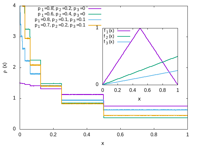
Figure 1: Steady state of the RDS given by Eq. (4) which evolves by choosing one of the three maps (shown in the inset) with probabilities $p_{1},p_{2},p_{3}.$

For the random map (4), we partition the domain $x\in[0,1]$ into infinitely many intervals labeled by $i=0,1,2,\dots,$ where the $i\textsuperscript{\text{th}}$ interval is defined as

$$I_{i}=\left[\frac{1}{2^{i+1}},\frac{1}{2^{i}}\right]$$ (5)

which has a width $w_{i}=2^{-i-1}.$ Clearly $\sum_{i=0}^{\infty}w_{i}=1.$ The set of widths $\{w_{i}\}$ can be represented by an infinite dimensional vector

$$\langle w|=\sum_{i=0}^{\infty}\frac{1}{2^{i+1}}\langle i|.$$ (6)

Let the initial distribution $\rho_{0}(x)$ be a piece-wise constant $c_{i}$ in interval $i$ represented by

$$|\rho_{0}\rangle=\sum_{i=0}^{\infty}c_{i}(0)|i\rangle~{}~{}{\rm and}~{}~{}\langle w|\rho_{0}\rangle=1,$$ (7)

where the last step ensures normalization, $\int_{0}^{1}dx\rho_{0}(x)=1=\sum_{i=0}^{\infty}\frac{c_{i}}{2^{i+1}}.$

Since the set of partitions is invariant under the action of the random map, the evolution of density is a Markov process,

$$|\rho_{t}\rangle=\ M^{t}|\rho_{0}\rangle$$ (8)

where $M$ is the Markov matrix,

$$M = \frac{p_{1}}{2}\sum_{j=0}^{\infty}(|j\rangle\langle 0|+|j\rangle\langle j+1|)+2p_{2}\sum_{j=1}^{\infty}|j\rangle\langle j-1|$$ (10)

$$~{}~{}~{}~{}~{}~{}+4p_{3}\sum_{j=2}^{\infty}|j\rangle\langle j-2|$$

If an invariant measure exists for such a random map, then it must be piecewise constant. This is because the Markov dynamics in Eq. (10) settles to a steady state, having a constant value, say $c_{i}$ for each interval. The steady state weight $\rho(x)$ can be represented by

$$|\rho\rangle=\sum_{i=0}^{\infty}c_{i}|i\rangle,$$ (11)

which must be a eigenvector of $M$ with unit eigenvalue, i.e., $M|\rho\rangle=|\rho\rangle.$ This condition leads to

$$c_{i}=4p_{3}c_{i-2}+2p_{2}c_{i-1}+\frac{p_{1}}{2}\left(c_{i+1}+c_{0}\right)$$ (12)

with boundary conditions $c_{-1}=0=c_{-2}.$ One can write this equation using a $3\times 3$ transfer matrix $T$ as,

$$|u_{i+1}\rangle=T|u_{i}\rangle-c_{0}|1\rangle$$ (13)

where,

$$T=\begin{pmatrix}\frac{2}{p_{1}}&-\frac{4p_{2}}{p_{1}}&-\frac{8p_{3}}{p_{1}}\\ 1&0&0\\ 0&1&0\end{pmatrix};|u_{i}\rangle=\left(\begin{array}[]{c}c_{i}\\ c_{i-1}\\ c_{i-2}\end{array}\right);|1\rangle=\left(\begin{array}[]{c}1\\ 0\\ 0\end{array}\right).$$ (14)

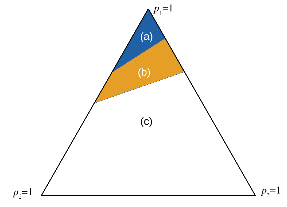
Figure 2: Phase diagram for RDS in Eq. (4): ACIM exists (or $\rho(x)$ is well-defined) in both the regions (a) and (b), whereas Pelikan’s criterion holds only in region (a) where $p_{3}<\frac{1}{7}(1-3p_{2}).$ ACIM does not exist in region (c); here $\rho(x)=\delta(x)$. The equation of the transition line, that separates regions (b) from (c) is $p_{3}=\frac{1}{3}(1-2p_{2}).$

The boundary condition $c_{-1}=0=c_{-2},$ sets the initial vector as $|u_{0}\rangle=c_{0}|1\rangle.$ By iterating (13) we get a solution,

$$|u_{i}\rangle=c_{0}\left(T^{i}-\sum_{j=0}^{i-1}T^{j}\right)|1\rangle.$$ (15)

Thus,

$$c_{i}=\langle 1|u_{i}\rangle=c_{0}\left(\langle 1|T^{i}|1\rangle-\sum_{j=0}^{i-1}\langle 1|T^{j}|1\rangle\right)$$ (16)

Now, the steady state weights $\{c_{i}\}$ can be calculated explicitly from knowing $c_{0}$ which can be obtained from the normalization condition of the steady state density and from $\langle 1|T^{i}|1\rangle$ which can be obtained from the eigensystem of the transfer matrix $T.$ $T$ has eigenvalues,

$$\lambda_{0}=2,\lambda_{\pm}=\frac{1}{p_{1}}\left(p_{2}+p_{3}\pm\sqrt{(p_{2}-p_{3})^{2}+4p_{3}(1-p_{3})}\right)$$ (17)

$${\rm with~{}right~{}eigenvectors}~{}|\sigma\rangle=\left(\begin{array}[]{c}\lambda_{\sigma}^{2}\\ \lambda_{\sigma}\\ 1\end{array}\right),\sigma=0,\pm.$$ (21)

The left eigenvectors $\langle\sigma|$ are orthonormal to $|\sigma\rangle,$ i.e., $\langle\sigma|\sigma^{\prime}\rangle=\delta_{\sigma,\sigma^{\prime}}$. Thus, $\langle 1|T^{i}|1\rangle=\sum_{\sigma}A_{\sigma}\lambda_{\sigma}^{i}$ where $A_{\sigma}=\langle 1|\sigma\rangle\langle\sigma|1\rangle.$ Note that $\sum_{\sigma}A_{\sigma}=1.$ Explicitly,

$$A_{\sigma}=\frac{\lambda_{\sigma}^{2}}{(\lambda_{\sigma}-\lambda_{\sigma^{\prime}})(\lambda_{0}-\lambda_{\sigma^{\prime\prime}})}~{}{\rm with}~{}\sigma^{\prime}\neq\sigma\neq\sigma^{\prime\prime}.$$ (22)

Using this in Eq. (16) and setting $\lambda_{0}=2$ we get

$$\frac{c_{i}}{c_{0}}=A_{0}+\sum_{\sigma=\pm}A_{\sigma}\left(\frac{2-\lambda_{\sigma}}{1-\lambda_{\sigma}}\lambda_{\sigma}^{i}-\frac{1}{1-\lambda_{\sigma}}\right)$$ (23)

Now, $c_{0}$ can be obtained from the normalization condition $\langle w|\rho\rangle=1;$ from Eq. (23),

$$1=\sum_{i=0}^{\infty}\frac{c_{i}}{2^{i+1}}=c_{0}A_{0}$$ (24)

$$\Rightarrow c_{0}=\frac{1}{A_{0}}=(1-\frac{\lambda_{+}}{2})(1-\frac{\lambda_{-}}{2})=3-\frac{2-p_{2}}{p_{1}}$$ (25)

Finally, the steady state weights are given by

$$c_{i}=1+\sum_{\sigma=\pm}\frac{A_{\sigma}}{A_{0}}\left(\frac{2-\lambda_{\sigma}}{1-\lambda_{\sigma}}\lambda_{\sigma}^{i}-\frac{1}{1-\lambda_{\sigma}}\right)$$ (26)

$c_{i}$ depends exponentially on $i,$ dominated by $\lambda_{+}^{i}$ for large $i$ as $\lambda_{+}>\lambda_{.}$ Whether it grows or decays, depends on the value of $\lambda_{+}.$ If $1<\lambda_{+}<2,$ then $c_{i}$ grows exponentially, but the weights can be normalized as $\sum_{i=0}^{\infty}\frac{\lambda_{+}^{i}}{2^{i+1}}$ remains finite. Thus, $c_{i}$ diverges as $i\to\infty$ (the intervals closer to $x=0$) when $\lambda_{+}>1,$ i.e., when

$$p_{3}>\frac{1}{7}(1-3p_{2}).$$ (27)

On the other hand when $\lambda_{+}>2,$ $\sum_{i=0}^{\infty}\frac{\lambda_{+}^{i}}{2^{i+1}}$ diverges and thus the distribution cannot be normalized. Note that $\lambda_{+}=2$ leads to $c_{0}=0$ in Eq. (25). The only solution is to set $c_{0}=0$, thereby making $c_{i}=0$ for all $i$ except $i\to\infty$ where $c_{i}$ diverges. This is the signature of the distribution $\delta(x)$.

We must mention that the condition (27) is the same as Pelikan’s criterion, Eq. (3) which states that an ACIM certainly exists when $p_{3}<\frac{1}{7}(1-3p_{2}).$ The region where $c_{i}$ diverges but the steady state weights are still normalizable, is not captured by the criterion.

A phase plot of the system illustrating the above is shown in Fig. 2. It is a ternary diagram as we have three variables $p_{1},p_{2},p_{3}$ which sum up to $1$. Each point in the interior and the boundary of the triangle represents a valid set of parameters. The regions (a) and (b) represent the regions where the system has a well defined PDF in the steady state. In region (c), the system always ends up with a steady state density of the form $\delta(x)$.

II.1.1 Transitions

This system shows a transition in behaviour as the value of $p_{1}$ is changed. This transition occurs due to a crossing in the eigenvalue spectrum. As stated before, generally, the steady state weights $c(i)$ behave as $c(i)\sim\lambda_{+}^{i}$ with $c(i)w(i)\sim\left(\frac{\lambda_{+}}{C}\right)^{i}$. As long as the latter sums up to a finite value, there is no issue. However, with change in $p$, there will be a $p^{*}$ that violates this. Beyond this $p^{*}$, the system always reaches the distribution $\delta(x)$. This is the main feature of most of the transitions discussed herein.

II.1.2 Simulations

Simulations were carried out by drawing a large number of samples from different initial distributions, usually a uniform random initial distribution, denoted by $U[0,1]$ and the second being the distribution of the squares of the random numbers from $U[0,1]$. After this, at each step, each sample is evolved and the final histogram is computed. A complete numerical example is shown in the Section II.4.

II.2 What we mean by ACIM

Existence of an absolutely continuous invariant measure (ACIM) refers to a well defined, measurable, steady state probability density function $\rho(x)$. The uniqueness refers to the fact that starting from any arbitrary initial distribution $\rho_{0}(x)$ of $x$ at $t=0,$ one must evolve to a unique steady state $\rho(x)$ in the $t\to\infty$ limit.

However, it must be emphasized that the initial density $\rho_{0}(x)$ must be measurable. To demonstrate this, we consider many different $\rho_{0}(x)$ and calculate the steady state density $\rho(x)$ for the random map Eq. (4) as shown in Fig. 3. The steady states obtained starting from $\rho_{0}(x)=\frac{1}{2\sqrt{x}}$ or $\rho_{0}(x)=U(0,1),$ are identical to the exact results obtained in Section II.1. However, when $\rho_{0}(x)=U(0.59,0.61)=g_{1}(x),$ i.e., when the initial distribution is uniform, having a width $\Delta x=0.02$ about $x=0.6,$ the resulting steady state, for small values of $x,$ exhibits some discrepancy from the exact results.

The surprising case is when $\rho_{0}(x)=\delta(x-a)$ which is not measurable. The resulting steady state $\rho(x)$ is now a series of $\delta$-functions. In Fig. (3) we demonstrate this by taking $a=0.6792$ as an example; the delta functions appearing in $\rho(x)$ are marked as vertical lines. Such a behavior necessarily indicates that, in general, the ensemble average and the time average are not the same in random dynamical systems.

In usual stochastic maps (defined by $x_{t+1}=f(x_{t})+\zeta_{t}$) or in other stochastic processes, one does not encounter this scenario; starting from any measurable initial distribution, or from a $\delta$-distribution, the system usually evolves to a unique steady state. The random dynamical system is special in the sense that, the evolution is deterministic and stochasticity appears only in making a choice of function out of many. For example, in Eq. (4), if one starts from $\rho_{0}(x)=\delta(x-a)$ with $a$ being a rational number, it is clear that in the subsequent evolution, $x_{t}$ cannot be an irrational number. Even when one starts from a irrational number, say $x_{0}=\frac{\pi}{4}$, it is not possible to get, say, $x_{t}=\frac{1}{\sqrt{\pi}}$ for any $t>0.$ On the other hand, if the initial distribution is measurable, then $x_{0}$ can be as close as we want to a predefined number and thus it can subsequently explore the neighborhood of any specific $x\in(0,1)$ densely, resulting in a measurable distribution whenever it exists.

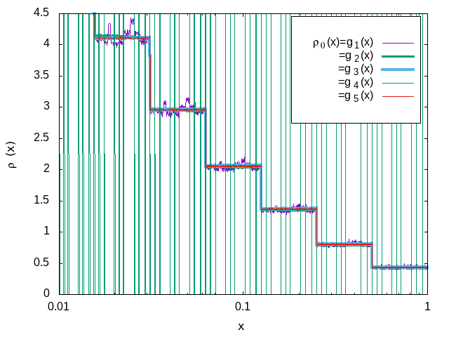
Figure 3: Stationary density function for RDS (4) for $p_{3}=0,p_{1}=0.6),$ with initial density $\rho_{0}(x)$ given by $g_{1}(x)=U(0.59,0.61)$ $g_{2}(x)=\frac{1}{2\sqrt{x}}$, $g_{3}(x)=2-|2x-1|$, $g_{4}(x)=\delta(x-.6792)$, $g_{5}(x)=U(0,1).$ All initial densities except $\rho(x)=g_{4}(x),$ which is not measurable, lead to a unique steady state.

II.3 Behaviour of the Mean at the Critical Point

In this section, we calculate the dependence of the mean $\langle x\rangle$ on $t,$ particularly at the critical point. To this end, we take a specific random map (4) with $p_{1}=p,p_{2}=1-p~{}\text{and}~{}p_{3}=0$ and calculate $\langle x\rangle$ analytically, near the critical threshold $p^{*}=\frac{1}{2}.$ For $p<p^{*},$ the ACIM ceases to exist. We set $p=\frac{1}{2}+\epsilon,$ so that the ACIM exists for $\epsilon>0.$ In this regime, we write

$$|\rho(t)\rangle=\sum_{j=0}^{\infty}c_{j}(t)|j\rangle$$ (28)

and study the asymptotic behaviour of $c_{j}(t).$ The mean $\langle x\rangle$ can be calculated explicitly as,

$$\langle x\rangle_{t}=\sum_{j=0}^{\infty}\int_{2^{-j-1}}^{2^{-j}}dx\;x\;c_{j}(t)=\frac{3}{8}\sum_{j=0}^{\infty}\frac{c_{j}(t)}{2^{2j}}.$$ (29)

Let the initial distribution be

$$|\rho(0)\rangle=\sum_{j=0}^{\infty}|j\rangle,~{}{\rm where~{}we~{}set}~{}c_{j}(0)=1\;\forall j.$$ (30)

The initial distribution is normalized, as $\langle w|\rho(0)\rangle=1.$ Since $|\rho(t)\rangle=M^{t}|\rho(0)\rangle,$ and

$$M=\frac{p}{2}\sum_{j=0}^{\infty}(|j\rangle\langle 0|+|j\rangle\langle j+1|)+2(1-p)\sum_{j=1}^{\infty}|j\rangle\langle j-1|,$$ (31)

we write $c_{j}(t)=\langle j|\rho(t)\rangle=\sum_{i=0}^{\infty}\langle j|M^{t}|i\rangle.$ Thus,

$$c_{j}(t+1)=\frac{p}{2}\left(c_{0}(t)+c_{j+1}(t)\right)+2(1-p)c_{j-1}(t).$$ (32)

This, along with Eq. (29) leads to

$$\langle x\rangle_{t+1}=\frac{1+3p}{2}\langle x\rangle_{t}-\frac{p}{2}c_{0}(t),$$ (33)

which can be solved by introducing a formal forward-time operator $\cap F$ that acts on $y_{t}$ as $\cap Fy_{t}=y_{t+1}.$

$$\langle x\rangle_{t}=\frac{p}{3p+1}\sum_{\tau=0}^{\infty}\left(\frac{2}{1+3p}\right)^{\tau}c_{t+\tau}(0).$$ (34)

Clearly, $\langle x\rangle_{t}$ depends only on $\{c_{t}(0)\}.$ To proceed further and to calculate $c_{t}(0),$ we set $p=\frac{1}{2}+\epsilon$ and calculate $c_{t}(0).$ From the structure of the matrix $M$ we find, to a linear order in $\epsilon,$

$$c_{t}(0)=2\epsilon+\frac{1-2\epsilon}{2^{t}}C_{\lfloor t/2\rfloor}^{t}$$ (35)

For large $t,$ we can replace $\lfloor t/2\rfloor$ by $t/2$, use Stirling’s approximation to write $\frac{C_{t/2}^{t}}{2^{t}}=\sqrt{\frac{2}{\pi t}},$ and replace the sum in Eq. (34) by an integral to get, for $p=\frac{1}{2}+\epsilon,$

$$\langle x\rangle_{t}=\frac{1+2\epsilon}{5+6\epsilon}2\epsilon+\frac{1-4\epsilon^{2}}{5+6\epsilon}\sqrt{\frac{2}{\pi}}\int_{0}^{\infty}d\tau\frac{1}{\sqrt{t+\tau}}\left(\frac{4}{5+6\epsilon}\right)^{\tau}$$ (36)

In the $t\to\infty$ limit, $\int_{0}^{\infty}d\tau\frac{z^{\tau}}{\sqrt{t+\tau}}\simeq\frac{1}{|\ln(z)|{\sqrt{t}}}.$ Thus, to a linear order in $\epsilon,$

$$\langle x\rangle_{t}=\frac{1}{5s}\sqrt{\frac{2}{\pi t}}+\left(\frac{2}{5}-6\frac{1+s}{25s^{2}}\sqrt{\frac{2}{\pi t}}\right)\epsilon,$$ (37)

where $s=\ln(\frac{5}{4}).$ When $\epsilon=0,$ i.e., at $p=p^{*},$ $\langle x\rangle_{t}\sim\frac{1}{\sqrt{t}}$ and for $\epsilon>0,$ $\langle x\rangle_{t}$ approaches a constant $\frac{2}{5}\epsilon$ as $t\to\infty.$

II.4 How to get $p^{*}$ numerically

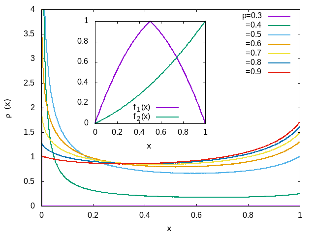
Figure 4: The steady state densities of the map in Eq. (41) shown in the inset, for different $p$. Clearly, for $p>0.4$ we have a well defined density everywhere while at $p=0.3$, $\rho(x)=\delta(x).$

Exact steady state measures can be obtained analytically for piecewise linear maps by using the Lasota-Yorke method introduced in Refs. LY ; Bowen . It is straightforward to generalize the methods to random maps which are piecewise linear. However, it is difficult to obtain the steady state measure for nonlinear maps analytically; thus, in most cases, one has to rely on numerical results. In this section, we discuss how to obtain $p^{*}$ for a class of bounded random maps.

Let us consider the following example.

$$f_{1}(x) = \left\{\begin{array}[]{ll}3x-2x^{2}&0\leq x\leq\frac{1}{2}\\ 1+x-2x^{2}&\frac{1}{2}<x\leq 1\end{array}\right.$$ (40)

$$f_{2}(x) = \frac{x}{2}(1+x)$$ (41)

$p_{1}=p$ and $p_{2}=1-p$

We simulated the map as follows and measured the steady state density $\rho(x)$ for different $p.$ We start from a initial value $x=x_{0},$ distributed uniformly in the interval $(0,1)$ and evolve the map for a large time $t=T$ and measured the distribution $\rho(x_{T}).$ The same is measured at $t=2T.$ We increase $T$ until $\rho(x_{2T})$ becomes indistinguishable from $\rho(x_{T})$. This ensures that,

$$\rho(x)\equiv\lim_{T\to\infty}\rho(x_{T}).$$ (42)

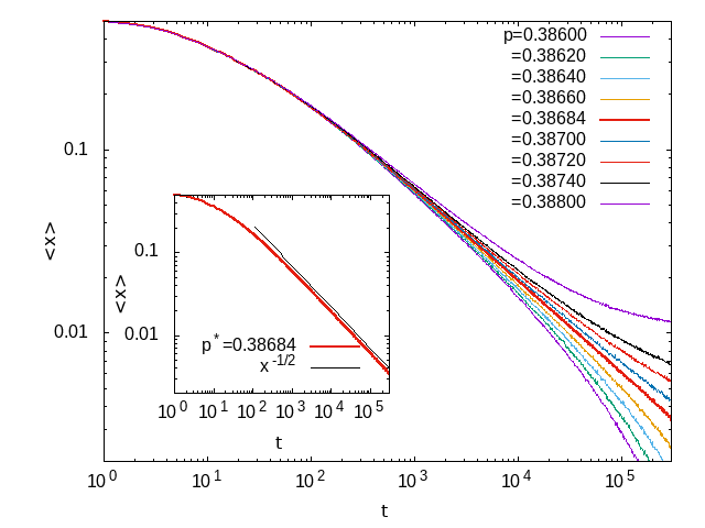
Figure 5: $\langle x\rangle$ versus $t$ for the RDS of Eq. (41) for different $p.$ When $p>p^{*},$ $\langle x\rangle$ attains a nonzero value as $t\to\infty,$ whereas $\langle x\rangle\to 0$ for $p<p^{*}.$ At $p=p^{*},$ $\langle x\rangle\sim t^{-\frac{1}{2}}.$ These facts helps up find $p^{*}=0.38684.$ The inset compares $\langle x\rangle$ versus $t$ with $t^{-\frac{1}{2}}$.

For the map defined in Eq. (41),

$$\Pi(x)=\left\{\begin{array}[]{ll}\frac{p}{3-4x}+2\frac{1-p}{1+2x}&~{}~{}~{}0\leq x\leq\frac{1}{2}\\ \frac{p}{4x-1}+2\frac{1-p}{1+2x}&~{}~{}~{}\frac{1}{2}<x\leq 1\end{array}\right.$$ (43)

Clearly $\Pi(x)<1$ for all values of $x\in(0,1),$ when $p>\frac{3}{5};$ thus, according to Pelikan’s criterion, there exists an ACIM $\rho(x)$ for this map when $p>\frac{3}{5}.$ In other words, if the invariant measure ceases to exist for some $p<p^{*}$ then $p^{*}$ must be smaller than $\frac{3}{5}.$ In Fig. 3, we have plotted $\rho(x)$ for different $p.$ For $p\geq 0.4,$ the steady state density $\rho(x)$ is a continuous and differentiable function, whereas for $p=0.3$ the steady state weight is concentrated at $x=0,$ i.e., $\rho(x)=\delta(x).$ Firstly, it verifies the fact that, when random maps have a common fixed point at $x=a$ which is stable for at least one of the maps, then $\rho(x)=\delta(x-a)$ whenever the ACIM ceases to exist. This also indicates that the threshold value $p^{*}$ is bounded in the interval $(0.3,0.4).$ In Fig. 5, we determine $p^{*}$ accurately from numerical simulations.

III The fixed point conjecture

In the previous section, we have seen that when the ACIM does not exist, the random map gets attracted to a common fixed point of all the mapping functions. For example, the random map $\{f_{1}(x)=1-|1-2x|,$ $f_{2}(x)=\frac{x}{2}\}$ which is a special case, $p_{3}=0~{}\text{and}~{}p_{1}=p=1-p_{2},$ of Eq. (4), the map is attracted to $x=0,$ when $p<p^{*}=\frac{1}{2},$ i.e., the resulting probability density is $\rho(x)=\delta(x).$ This feature appears to be common to any random map. We conjecture that,if the ACIM ceases to exist for any random map which has $N$ common fixed points at $x=\{a_{\nu}\},\nu=1,2,\dots,N,$ each one being attractive (or stable) for at least one of the constituting maps, then the density in the $t\to\infty$ limit will be

$$\rho(x)=\sum_{\nu=1}^{N}C_{\nu}\delta(x-a_{\nu})~{}{\rm with}~{}\sum_{\nu=1}^{N}C_{\nu}=1,$$ (44)

where $C_{\nu}$ are constants that depend on initial density $\rho_{0}(x).$

There are several questions which need clarification, even for $N=1.$ We will discuss the $N\geq 2$ case in the next section. So far the RDS we considered have a common fixed point which is attractive for one of the maps in ${\cal S},$ but this fixed point is incidentally a boundary point of the interval on which maps in ${\cal S}$ are defined. To strengthen the conjecture, we must show that the RDS, in this situation is attracted to the fixed point, not to a boundary. In other words, we must show that when the CFP is $x=a_{1}\neq 0,$ in absence of ACIM the RDS leads to a steady state $\rho(x)=\delta(x-a_{1}).$ We discuss this in section III.1.

One may also raise the following question. The CFP is repulsive or unstable for some of the constituting maps, but in the examples studied here, the ‘repulsive power’ may not be sufficient to overcome the stability enforced by other maps. To strengthen the conjecture, we must show that irrespective of the strength of repulsion, the RDS gives rise to a localized steady state density at the CFP whenever the fixed point is stable for one of the constituting maps. We discuss this in Section III.2.

III.1 Common fixed point in the bulk

In this section, we show that the RDS gets attracted to the common fixed point, irrespective of whether it is a boundary of the interval. Let us consider a random map that evolves by choosing one of the functions in ${\cal S}=\{f_{1}(.),f_{2}(.)\}$ with probabilities $p$ and $(1-p)$ respectively. The functions are

$$f_{1}(x)=1-|1-2x|,~{}~{}~{}f_{2}(x)=1-\frac{x}{2}.$$ (45)

Clearly, both the functions have a fixed point at $x=a_{1}=\frac{2}{3},$ which is repulsive for $f_{1}(.)$ and attractive for $f_{2}(.)$. Notice that the map can be converted to a Markov map by converting the interval $[0,1]$ into two sub-intervals labeled by an index $\sigma=\pm:$ the interval $[0,\frac{2}{3}]$ where $x<a_{1}$ is denoted by $\sigma=-$ and the rest $[\frac{2}{3},1]$ is denoted as $\sigma=+.$ Each of these sub-intervals, like before, is now divided into a set of infinite intervals $I_{i,\sigma},$ with $i=0,1,2,\dots,\infty.$

$$I_{i,-} =\left[\,\frac{2}{3}\left(1-\frac{1}{4^{i}}\right),\frac{2}{3}\left(1-\frac{1}{4^{i+1}}\right)\right]$$ (46)

$$I_{i,+} =\left[\,\frac{2}{3}+\left(\frac{1}{3}\right)\left(\frac{1}{4^{i+1}}\right),\frac{2}{3}+\left(\frac{1}{3}\right)\left(\frac{1}{4^{i}}\right)\right]$$ (47)

The width of the intervals are $w_{i,+}=\frac{1}{2}w_{i,-}={4^{-(i+1)}}.$ One can check that this interval structure is invariant under action of the mapping functions,

$$f_{2}(I_{i,-})=I_{i,+};~{}~{}~{}f_{2}(I_{i,+})=I_{i+1,-}~{}~{}\forall~{}~{}k\geq 0$$ (48)

$$f_{1}(I_{i,-})=I_{i-1,+};~{}~{}~{}f_{1}(I_{i,+})=I_{i,-}~{}~{}\forall~{}~{}k\geq 0$$ (49)

$$~{}~{}{\rm and}~{}~{}f_{1}(I_{0,-})=\bigcup_{i=0}^{\infty}\left[I_{i,-}\cup I_{i,+}\right]$$ (50)

These equations help us in writing a Markov evolution on the intervals, which leads to a steady state density $\rho(x)$ which is a piecewise constant $c_{i,\sigma}$ in each interval $I_{i,\sigma}.$ The condition of stationarity demands $c_{i,\sigma}$s to obey, for $i>0,$

$$c_{i,-} = \frac{p}{2}\left(c_{0,-}+c_{i,+}\right)+2(1-p)c_{i-1,+}$$ (51)

$$c_{i,+} = \frac{p}{2}(c_{0,-}+c_{i+1,-})+2(1-p)c_{i,-}$$ (52)

$${\rm and}~{}~{}c_{0,-} = \frac{p}{2}(c_{0,-}+c_{0,+}).$$ (53)

Now we solve for $c_{i,+}$ from the second equation and use it in the first to get,

$$c_{i+1,-}=T_{11}c_{i,-}+T_{12}c_{i-1,-}+\alpha c_{0,-},$$ (54)

where $T_{11}=\frac{4}{p^{2}}\left(1-2p(1-p)\right),T_{12}=-4^{2}\frac{(1-p)^{2}}{p^{2}}$ and $\alpha=-3\frac{2-p}{p}.$ This equation can be expressed in matrix form, $|u_{i+1}\rangle=T|u_{i}\rangle+\alpha c_{0-}|1\rangle,$ where

$$|u_{i}\rangle=\begin{pmatrix}c_{i,-}\\ c_{i-1,-}\end{pmatrix},|1\rangle=\begin{pmatrix}1\\ 0\end{pmatrix}~{}~{}{\rm and}~{}~{}T=\begin{pmatrix}T_{11}&T_{12}\\ 1&0\end{pmatrix}.$$ (55)

This matrix equation is similar to Eq. (13) and its solution is discussed there in detail. Following similar steps, and noting that the eigenvalues of $T$ are $\{\lambda_{0}=4,\lambda_{1}=4\left(\frac{1-p}{p}\right)^{2}\}$, we obtain a solution

$$c_{i,-}=c_{0,-}\left(\frac{1}{3p-2}\right)\left(p-2(1-p)\lambda_{1}^{i}\right)$$ (56)

Using these results in Eq. (53),

$$c_{i,+}=c_{0,-}\left(\frac{1}{p(3p-2)}\right)\left(p^{2}-4(1-p)^{2}\lambda_{1}^{i}\right).$$ (57)

Both $c_{i,\sigma}$ depend on $c_{0,-}$ which can be determined from the normalization condition

$$\sum_{\sigma=\pm}\sum_{i=0}^{\infty}c_{i,\sigma}w_{i,\sigma}=1.$$ (58)

In fact, $c_{0,-}=2-\frac{1}{p}.$

From the steady state solution, we see immediately that there are three distinct regions. When $p>\frac{2}{3}$, $\lambda<1$ and $c_{i,\sigma}$ are finite for all $i;$ thus we have a well defined steady state measure. In the region $\frac{1}{2}<p<\frac{2}{3},$ we have $1<\lambda<4$ which indicates that $c_{i,\sigma}$ diverges as $i\to\infty,$ i.e., when $x$ approaches the fixed point $a_{1}=\frac{2}{3}.$ However, $c_{i,\sigma}w_{i,\sigma}\sim\left(\frac{\lambda}{4}\right)^{k},$ and it is smaller than unity for any $i.$ Thus, even when $c_{i,\sigma}$ diverges at $x=\frac{2}{3},$ the steady state density is normalizable, as the normalization condition Eq. (58) gives rise to a finite $c_{0,-}$. Finally $\lambda$ becomes larger than $4$ in the region $p<\frac{1}{2}$ and in this region, all $c_{i,\sigma}$ except $c_{\infty,\sigma}$ must vanish. In other words, for $0<p<\frac{1}{2},$ the density is $\rho(x)=\delta(x-a_{1}).$

In Fig. 6 we show the steady state distribution in three different regimes.

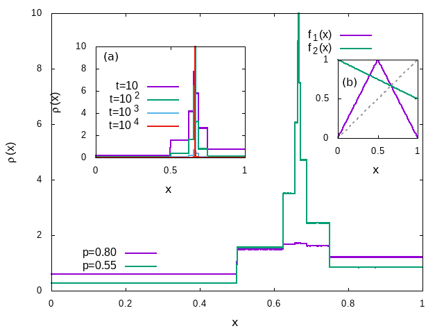
Figure 6: The steady state density $\rho(x)$ of the RDS, consisting two maps defined in Eq. (45) and plotted in (b). For $p=0.8$, $\rho(x)$ is is finite everywhere, while at $p=0.55$ it diverges at $x=\frac{2}{3}$ but it is normalized. (a) For $p=0.41,$ $\rho(x),$ plotted for $t=10,10^{2},10^{3},10^{4}$ indicate that it slowly converges to $\delta(x-\frac{2}{3}).$

III.2 CFP is strongly repulsive

In the earlier examples we have seen that the system, in absence of an ACIM, gets attracted to the common fixed point, even when the fixed point is repulsive (or unstable) for some maps. If the CFP is attractive for all maps then the attraction of the RDS towards it is not surprising. One may doubt that, those examples where the fixed point is unstable, the ‘repulsive power’ may not be strong enough to push the system away from the fixed point. By ’repulsive power’ here, we refer to the magnitude of the derivative of the unstable map at the fixed point. Let us consider a RDS consisting of two functions,

$$f_{1}(x)=\left\{\begin{array}[]{ll}2^{\nu}x&~{}~{}~{}0\leq x\leq\frac{1}{2^{\nu}}\\ 1-|1-2x|&~{}~{}~{}\text{else}\end{array}\right.$$ (61)

$${\rm and}~{}f_{2}(x)=\frac{x}{2}.$$ (62)

As before $f_{1}(x)$ is chosen with probability $p$ while $f_{2}(x)$ is chosen with probability $1-p$. $x=0$ which is a CFP of both maps is a stable fixed point of $f_{2}(.)$ and is unstable for $f_{1}(.).$ The slope of the repulsive map at $x=0$ can be considered as the ’repulsive power’, which is $2^{\nu}$ here. This must be compared with the ‘attractive power’ of $f_{2}(.)$ which the inverse of the slope at $x=0.$ Thus, for $\nu>1$ the repulsion from $x=0$ is much stronger than the attraction towards $x=0.$ We will show that the RDS is attracted to the CFP even when $\nu\to\infty;$ this result, thus, supports the fixed point conjecture very strongly.

We partition the domain $I=[0,1]$ into intervals $I_{i}=[\frac{1}{2^{i+1}},\frac{1}{2^{i}}]$ of width $w_{i}=1/2^{i+1},$ as in Eq. (5). The dynamics of this RDS can be mapped to a Markov process on the intervals, where the density at time $t$ is $|\rho(t)\rangle=\sum_{i=0}^{\infty}c_{i}(t)|i\rangle$. The coefficients evolve to a steady value $c_{i}(\infty)\equiv c_{i}$ as $t\to\infty.$ In the steady state, $c_{i}$s obey,

$$i=0 :~{} c_{0}=\frac{p}{2}(c_{0}+c_{1})+\frac{p}{2^{\nu}}c_{\nu}$$ (63)

$$0\leq i<\nu :~{} c_{i}=\frac{p}{2}\left(c_{0}+c_{i+1}\right)+\frac{p}{2^{\nu}}c_{i+\nu}+2(1-p)c_{i-1}$$ (64)

$$i\geq\nu :~{} c_{i}=\frac{p}{2}c_{0}+\frac{p}{2^{\nu}}c_{i+\nu}+2(1-p)c_{i-1}$$ (65)

along with a normalization condition $\sum_{i=0}^{\infty}c_{i}w_{i}=1.$ To solve this, we note that the general solution of $c_{i}$ must come from the last line of the above equation, on which first two equations act as boundary conditions. Setting $c_{i}=(2z)^{i},$ reduces the last line of Eq. (65) to a $(\nu+1)$-order polynomial when terms of the ${\cal O}(\frac{1}{2^{i}})$ are dropped,

$$z=pz^{\nu+1}+1-p,$$ (66)

which has roots, say $z_{\alpha},$ with $\alpha=1,2,\dots,\nu+1.$ Note, that $z=1$ always solves Eq. (66) for any $p.$ In fact it is the largest positive solution for any value of $p$, because, for $z>1$ the r.h.s. of Eq. (66) is larger than $z$ (the l.h.s). Moreover, Descartes’ sign rule suggests that the polynomial has at most two positive solutions for any $\nu,$ and at most one negative solution if $\nu$ is even. The general solution of $c_{i}$ is

$$c_{i}=A_{1}(2z_{1})^{i}+A_{2}(2z_{2})^{i}+\dots,$$ (67)

where we keep only two dominant contributions coming from the two positive roots of (66), $z_{1}=1$ and $z_{2}$ which is smaller than $z_{1}$ when $p$ is large. When $p$ is decreased beyond some threshold, say $p=p^{*},$ $z_{2}$ becomes larger than $z_{1}$ and then $\sum_{i=0}^{\infty}c_{i}w_{i}$ diverges breaking the normalization condition, leading to nonexistence of ACIM.

At $p=p^{*}$ we have $z_{2}=1=z_{1};$ thus at this value the characteristic polynomial (66) must have the form $(z-1)^{2}h(z),$ whose derivative at $z=1$ must vanish. Differentiating Eq. (66) and setting $z=1$ at $p=p^{*}$ we get,

$$p^{*}=\frac{1}{\nu+1}$$ (68)

It is clear now, that for any value of the repulsion strength $\nu,$ irrespective of how large it is, there always exist a region $p\in(0,p^{*})$ where the RDS is attracted to the common fixed point (here $x=0$).

We end this discussion here, leaving out the exact results which can be obtained using from Eq. (65) following the steps described in detail for $\nu=1,$ i.e., Eq. (4) with $p_{3}=0.$ One must remember that the general solution $c_{i}=\sum_{\alpha=1}^{\nu+1}A_{\alpha}(2z)^{\alpha}$ has $\nu+1$ arbitrary constants $\{A_{\alpha}\}$ which must be fixed by using the $\nu$ equations written as first two lines in (65) and the normalization condition. In addition physical constraints (like $c_{i}$ must be real) may force some of $A_{\alpha}$ to vanish.

The following comment is in order. The criteria for an RDS to have an ACIM has also been discussed before Sato2019 ; 19 . In particular, Ott et. al. 19 argued that ACIM ceases to exist when the mean Lyapunov Exponent $\overline{\lambda}$ of the system becomes negative. For the RDS (65), the Lyapunov exponents of the mapping functions $f_{1,2}(x)$, sufficiently close to $x=0$ are respectively $\lambda_{1}=\nu,\lambda_{2}=-1$ and their average $\bar{\lambda}=p\lambda_{1}+(1-p)\lambda_{2}$ becomes negative when $p<\frac{1}{1+\nu},$ which is consistent with Eq. (68). Note that, this argument would suggest that when $f_{2}(x)$ is modified, say to $f_{2}(x)=\frac{x}{2}+\frac{1}{4}$ having the same Lyapunov exponent, then ACIM ceases to exist for $p<\frac{1}{1+\nu}.$ Clearly, the RDS in this case will not be attracted to the fixed point $x=0;$ this happens only when there is a common fixed point which is attractive for at least one map.

IV RDS with TWO common fixed points

In the previous section we have seen that, if the mapping functions have a common fixed point which is attractive for at least one function, then the iterates of the random map generically reach this fixed point when the ACIM ceases to exist. What happens if the mapping functions have more than one CFP, each one stable for at least one function? Will this RDS reach any of the fixed points with equal probability? We investigate this scenario here in detail.

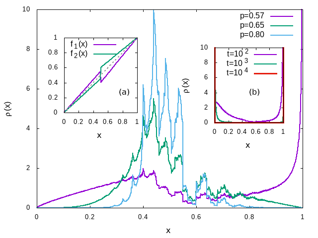
Figure 7: Steady states of the RDS (69) for different $p.$ The mapping functions are shown in (a). Clearly ACIM exists for $p>0.55$. (b) $\rho_{t}(x)$ for $p=\frac{1}{2}$ and $t=10^{2},10^{3},10^{4};$ clearly it approaches to $A\delta(x)+(1-A)\delta(x-1)$ as $t\to\infty$.

To this end, we consider an RDS with $K=2,$ with the mapping functions,

$$f_{1}(x)=\left\{\begin{array}[]{ll}(1+\alpha)x&~{}~{}~{}0\leq x\leq\frac{1}{2}\\ (1+\beta)x-\beta&~{}~{}~{}\frac{1}{2}<x\leq 1\end{array}\right.$$

and

$$f_{2}(x)=\left\{\begin{array}[]{ll}(1-\alpha)x&~{}~{}~{}0\leq x\leq\frac{1}{2}\\ (1-\beta)x+\beta&~{}~{}~{}\frac{1}{2}<x\leq 1\end{array}\right.,$$ (69)

which is plotted in the inset of Fig. 7 for $\alpha=0.1,\beta=0.2.$ Clearly $x=0,1$ are the common fixed points of both maps; both are unstable for $f_{1}(x)$ and stable for $f_{2}(x).$ For this random map,

$$\Pi(x)=\left\{\begin{array}[]{ll}\frac{p}{1+\alpha}+\frac{1-p}{1-\alpha}&~{}~{}~{}0\leq x\leq\frac{1}{2}\\ \frac{p}{1+\beta}+\frac{1-p}{1-\beta}&~{}~{}~{}\frac{1}{2}<x\leq 1\end{array}\right.$$ (70)

Thus Pelikan’s criterion suggests that the ACIM certainly exists when $p>p^{*}_{2}=\frac{1}{2}(1+\textrm{Max}\{\alpha,\beta\});$ for $\alpha=0.1,\beta=0.2,p^{*}_{2}=0.60.$ In Fig. 7 we have plotted $\rho(x)$ for different values of $p.$ It turns out that for $p<p^{*}=0.55,$ $\rho_{t}(x)$ develops substantial weight near the fixed points $x=0,1$ as $t\to\infty.$ This is shown in Fig. 7 (b) , for $p=0.5.$ Thus, for $p<p^{*}$ the steady state weight is not measurable, and it is given by,

$$\rho(x)=A\delta(x)+\left[1-A\right]\delta(1-x),$$ (71)

where the weight $A$ is yet to be determined.

IV.1 Fixed point conjecture: two CFPs

We believe that this is a very general result. Since both fixed points are attractive for some mapping function, starting from any initial value $x=x_{0}$ the random map has a nonzero probability to reach the fixed point, but it can always be pushed away by the other mapping function which is repulsive. Clearly when the repulsion is strong enough, i.e., when $p$ is large enough in Eq. (69), $x_{t}$ cannot stabilize at the fixed point and it spreads over the interval, giving rise to an unique invariant measure.

Now, the question is to determine $A.$ In fact $A(p),$ which is the weight of $\delta(x)$ can be interpreted as the total probability of reaching the fixed point $x=0,$ starting from any arbitrary initial value. This reminds us the hitting problem Feller of a simple random walk on a one dimensional lattice defined by sites $i=0,1,\dots,L;$ the probability that the walker, starting from $i=n,$ will reach the origin before hitting $L$ is $Q_{L}(n)=1-\frac{n}{L}.$

In dynamical systems, we have a continuous variable $x$ that evolves with discrete time. Thus an iterate can come arbitrarily close to the fixed point, but it will never hit it in any finite time. The question of reaching a fixed point, say $x=0$, is only a limiting procedure of $x_{t}$ becoming smaller than a predefined small number $\epsilon.$

For the random map given in Eq. (69), let us define $Q(w;p,\epsilon)$ as the probability that starting from an initial value $x_{0}=w\in(\epsilon,1-\epsilon),$ $x_{t}$ decreases below $\epsilon$ first time at $t=T$ without exceeding the value $1-\epsilon$ (i.e., $x_{T}<\epsilon$ and $x_{t}<1-\epsilon~{}~{}~{}~{}\forall~{}~{}1<t<T$). Then

$$A(p)=\lim_{\epsilon\to 0}\int_{\epsilon}^{1-\epsilon}dw~{}Q(w;p,\epsilon).$$ (72)

An interesting limiting case of the random map defined by Eq. (69) is when $\alpha=1=\beta;$ the evolution is given by

$$x_{t+1}=\left\{\begin{array}[]{ll}2x_{t}~{}{\rm mod}~{}1&{\rm prob.}\;p\\ \lfloor x_{t}\rceil&{\rm prob.}\;1-p\end{array}\right.,$$ (73)

where $\lfloor.\rceil$ is the nearest integer function. Thus, with probability $p$, the map evolves using the first function or otherwise hits the fixed points, $0$ (or $1$) if $x_{t}$ is less (greater) than $\frac{1}{2}.$

First let us consider the $p=1$ case. Then the evolution is deterministic, $x_{t+1}=2x_{t}$ mod $1.$ We now show that, in this case, $\rho_{t}(x)$ can be determined exactly if the starting density $\rho_{0}(x)$ is a piecewise constant in the interval defined as follows. Let us partition the domain $x\in(0,1)$ into infinitely many intervals labeled by $i=0,1,2,\dots,$ where the $i^{th}$ interval defined as $x\in(2^{-i-1},2^{i})$ has a width $w_{i}=2^{-i-1}.$ Clearly $\sum_{k=0}^{\infty}w_{i}=1.$ The corresponding infinite dimensional vector is represented by

$$\langle w|=\sum_{i=0}^{\infty}\frac{1}{2^{i+1}}\langle i|.$$ (74)

Let the initial distribution $\rho_{0}(x)$ be piecewise constant $c_{i}$ in interval $i$, represented by

$$|\rho_{0}\rangle=\sum_{i=0}^{\infty}c_{i}(0)|i\rangle~{}~{}{\rm and}~{}~{}\langle w|\rho_{0}\rangle=1,$$ (75)

where the last step ensures normalization, $\int_{0}^{1}dx\rho_{0}(x)=1=\sum_{i=0}^{\infty}\frac{c_{i}}{2^{i+1}}.$

Since the set of partitions is invariant under the action of the random map, the evolution of the density is a Markov process,

$$|\rho_{t}\rangle=\ M^{t}|\rho_{0}\rangle$$ (76)

where $M$ is the Markov matrix,

$$M=\frac{1}{2}\sum_{i=0}^{\infty}\left(|i\rangle\langle 0|+|i\rangle\langle i+1|\right)~{}~{}~{}~{}~{}~{}~{}$$ (77)

We may expand $|\rho_{t}\rangle$ as

$$|\rho_{t}\rangle=\sum_{i=0}^{\infty}c_{i}(t)|i\rangle~{}~{}{\rm where}~{}~{}c_{i}(t)=\langle i|M^{t}|\rho_{0}\rangle$$ (78)

and now the task is to find $c_{i}(t).$ It is easy to see from the structure of the matrix that

$$\langle i|M^{t}=\frac{1}{2^{t}}\langle i+t|+\sum_{n=0}^{t-1}\frac{1}{2^{n+1}}\langle n|$$ (79)

This equation necessarily ensures that the normalization $\langle w|M^{t}|\rho_{0}\rangle=1$ is preserved at all $t\geq 0.$ Thus,

$$c_{i}(t)=\langle i|M^{t}|\rho_{0}\rangle=\frac{c_{i+t}(0)}{2^{t}}+\sum_{n=0}^{t-1}\frac{c_{n}(0)}{2^{n+1}}.$$ (80)

This equation is crucial to us as it explicitly determines how the weights in each interval evolve with time, starting from the initial distribution $|\rho_{0}\rangle\equiv\{c_{i}(0)\}.$ When $\{c_{i}(0)=1\},$ which is normalized as $\langle w|\rho_{0}\rangle=1,$ then from (80) we get $\{c_{i}(t)=1\}$ for all $t\geq 0.$ Thus $\sum_{k=0}^{\infty}|k\rangle$ is an eigenstate of the Markov matrix $M$ with eigenvalue $1$, and it is the steady state of this random map. Note that Pelikan’s criterion predicts that for $p=1$, there is an invariant measure.

Let us consider another normalized initial density,

$$|\rho_{0}\rangle=\sum_{k=0}^{\infty}c_{i}(0)|i\rangle~{}{\rm where}~{}c_{i}(0)=(2-{\sqrt{2}})2^{i/2}$$ (81)

In this case, from Eq. (80) we get,

$$c_{i}(t)=1+2^{-t/2}\left(c_{i}(0)-1\right).$$ (82)

Thus, the random map evolves to its steady state $\sum_{k=0}^{\infty}|k\rangle$ as $t\to\infty.$

With all these information in hand, we now go to $p<1$ case. For any $p<1,$ Pelikan’s criterion fails. Now, the random map iterate either chooses with probability $p$ to evolve as $x_{t+1}=2x_{t}$ mod $1$ or with probability $1-p$, it reaches one of the fixed points - the integer which is nearest to $x_{t}$ and stays there. Thus, in the $t\to\infty$ limit, it will certainly reach one of these fixed points, resulting in

$$\rho_{\infty}(x)=A\delta(x)+\left(1-A\right)\delta(1-x).$$ (83)

How do we determine $A,$ the fraction of all evolving random maps that hit the fixed point $x=0$? Does it depend on the initial density $\rho_{0}(x)$?

The maps which survive the fixed point until $t$ have followed dynamics $x_{t+1}=2x_{t}$ mod $1$ discussed in the previous example. Since the survival probability at $t$ is $p^{t},$ for any initial density $|\rho_{0}\rangle=\sum_{k=0}^{\infty}c_{k}(0)|k\rangle$ which is piecewise constant, we have (from Eq. (80)) the survival weight

$$c_{i}(t)=p^{t}\left(\frac{c_{i+t}(0)}{2^{t}}+\sum_{n=0}^{t-1}\frac{c_{n}(0)}{2^{n+1}}\right).$$ (84)

The fraction of maps which hit the fixed point $x=1$ exactly at time $t$ is $(1-p)$ times the fraction of those that survive until $t,$ which is simply $\frac{1}{2}(1-p)c_{0}(t);$ here we set $i=0$, as the fixed point $x=1$ is reached from only the $0^{th}$ interval $(\frac{1}{2},1),$ and the factor $\frac{1}{2}$ is the width of $0^{th}$ interval. Thus, the total fraction of maps which are collected at $x=1$ is,

$$1-A = \frac{1-p}{2}\sum_{t=0}^{\infty}c_{0}(t)$$ (85)

$$= \frac{1-p}{2}\sum_{t=0}^{\infty}p^{t}\left[\frac{c_{t}(0)}{2^{t}}+\sum_{n=0}^{t-1}\frac{c_{n}(0)}{2^{n+1}}\right].$$ (86)

When the initial state is $|\rho_{0}\rangle=\sum_{i=0}^{\infty}|i\rangle,$ i.e, when $\{c_{i}(0)=1\},$ we get $A=\frac{1}{2}$ for all $p<1.$ On the other hand, when $|\rho_{0}\rangle$ is given by Eq. (81)(we refer to it as initial density -I) we get

$$A=1-\left(\frac{1}{\sqrt{2}}-\frac{1}{2}\right)\frac{2-p}{{\sqrt{2}}-p}.$$ (87)

Clearly, it appears that $A$ depends on the initial condition. Let us consider another example, initial density-II, where $|\rho_{0}\rangle=\sum_{i=0}^{\infty}c_{i}|i\rangle$ with

$$c_{0}=2-\frac{a}{3};~{}~{}c_{i}=\frac{a}{2^{i}}.$$ (88)

In this case, we get

$$A=\frac{p}{2}+a\left(\frac{2}{4-p}-\frac{1+p}{3}\right)$$ (89)

In Fig. 8 we have compared the variation of $A$ as a function of $p,$ obtained from numerical simulation of the RDS with different initial densities I and II, with corresponding exact results obtained in Eqs. (87) and (87). It is not surprising that the value of $A$ depends on the initial conditions; it is a natural consequence of the nonexistence of the ACIM.

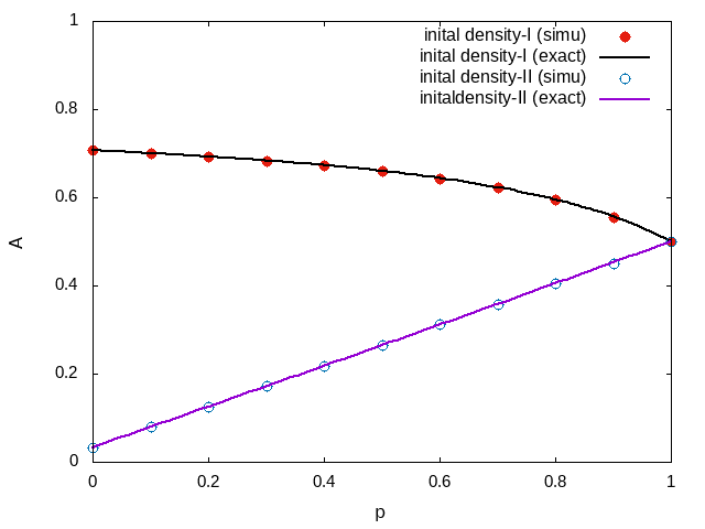
Figure 8: For the RDS (73) ACIM does not exist for any $0<p<1$ and the system hits the fixed points $x=0,1$ with probabilities $A,1-A$ respectively. The plot shows $A$ as a function of $p$ two initial densities I, and II (see text for details). Data from numerical simulations (symbols) are compared with respective exact results (87), (89). Here for initial density -II, in (88), we take $a=0.2.$

This method of calculating the weight $A$ is not possible when initial conditions are not piecewise constants in intervals which are consistent with the natural partitioning of the the random map in question. In the following we introduce another method.

IV.2 Mapping to hitting problems

When an RDS has two common fixed points, in absence of ACIM, the system gets attracted to one of them. This phenomenon is similar to the hitting problem in random walks. On a one dimensional lattice with two absorbing boundaries, the probability that the walker hits one of the boundaries before hitting the other is formally known as the hitting problem and is well studied. For a simple unbiased random walk, starting from $x=w$, the probability of hitting $x=0$ before hitting $x=L$ is $Q_{rw}(w)=1-w/L.$ A simple generalization, which will be useful here, follows.

Starting from $x_{l}<w<x_{r}$ the probability that the walker hits the left boundary $x_{l}$ before hitting the right one $x_{r}$ is $Q_{rw}(w)=1-(x-x_{l})/(x_{r}-x_{l}).$ The random walks on a lattice can be considered as a random dynamical system of two integer functions

$$f_{1}(x)=x+1~{}~{}{\rm and}~{}f_{2}(x)=x-1,$$ (90)

chosen with probability $p$ and $1-p$ respectively. The RDS are, however, different from simple random walks as the dynamical variable $x$ is real and during evolution $x_{t}$ cannot hit $0$ or $1$, although it can come infinitesimally close to the fixed points $x=0,1.$ Thus, hitting the fixed point in RDS can be mapped to hitting problem if we explicitly force the evolution to stop when $x$ goes below a predefined small parameter $\epsilon$ or when $x>1-\epsilon.$ And eventually, we take $\epsilon\to 0$ limit to get the probability of hitting one of the fixed points.

Without loss of generality, we take the fixed points to be $x=0,1$ and define $Q(w,\epsilon)$ as the probability that starting from $\epsilon<w<1-\epsilon$ at $t=0$ (i.e., $x_{0}=w$), $x_{t}$ for some $t$ goes below $\epsilon$ before crossing the value $1-\epsilon.$ Since starting from $x_{0}=w,$ the RDS evolves to $x_{1}=f_{k}(w)$ with probability $p_{k},$ we must have

$$Q(w,\epsilon)=\sum_{k=1}^{K}p_{k}Q(f_{k}(w),\epsilon);~{}~{}Q(w)\equiv\lim_{\epsilon\to 0}Q(w,\epsilon).$$ (91)

For $K=2$ RDS with $p_{1}=p=1-p_{2},$ we have

$$Q(w,\epsilon)=pQ(f_{1}(w),\epsilon)+(1-p)Q(f_{2}(w),\epsilon).$$ (92)

Interestingly, for any symmetric RDS defined by $f_{1,2}(x)=x\pm d(x)$ we immediately see that

$$Q(w,\epsilon)=1-\frac{w-\epsilon}{1-2\epsilon}$$ (93)

solves Eq. (92) for $p=1/2.$ Note that $Q(w,\epsilon)$ is the same as the probability that an unbiased walker starting from $x=wL,$ ends up at $\epsilon L$ without hitting $(1-\epsilon)L.$ For $p\neq\frac{1}{2},$ and for generic random maps which are not symmetric, calculating $Q(w,\epsilon)$ exactly may not be possible. However, Eq. (91) has an advantage that $Q(w,\epsilon)$ can be converted to a differential equation, when the parameters of the map are small. In absence of exact results like the one we have obtained in the previous section for RDS in Eq. (69), equation (91) is indeed very helpful which we demonstrate below.

Let us consider the RDS defined in Eq. (69) where we have calculated exactly that, in absence of ACIM, the system approaches the fixed point $x=0$ with probability $A.$ The value of $A$ depends on $p$ and the initial distribution $\rho_{0}(x).$ For $\alpha=1=\beta$ we have shown analytically that, for all $0<p<1$, the steady state density is $\rho(x)=(1-A)\delta(x)+A\delta(1-x)$ with $A=\frac{1}{2}$ when $\rho_{0}(x)$ is uniformly distributed in $(0,1);$ for some other $\rho_{0}(x),$ the value of $A$ has also been obtained in Eqs. (87) and (89). In fact $A$ is related to the hitting probability $Q(x,\epsilon)$ by the relation,

$$A=\lim_{\epsilon\to 0}\int_{\epsilon}^{1-\epsilon}dxQ(x,\epsilon)\rho_{0}(x)\equiv\int_{0}^{1}dxQ(x)\rho_{0}(x).$$ (94)

To calculate the value of $A,$ let us consider the RDS defined in Eq. (69); following Eq. (91) we get

$$Q(w,\epsilon)=\begin{cases}p~{}Q(\left(1+\alpha\right)w,\epsilon)+\bar{p}Q(\left(1-\alpha\right)w,\epsilon)&\text{if $x<\frac{1}{2}$}\\ p~{}Q(\left(1+\beta\right)w-\beta,\epsilon)&\\ ~{}~{}~{}~{}~{}+\bar{p}~{}Q(\left(1-\beta\right)w+\beta,\epsilon)&\text{else.}\end{cases}$$ (95)

Some specific cases are exactly solvable. For $p=\frac{1}{2},$ since the constituting functions of the RDS Eq. (69) are of the form $\{f_{1}(x)=x+d(x),f_{2}(x)=x-d(x)\}$ with

$$d(x)=\begin{cases}\alpha x&0\leq x\leq\frac{1}{2}\\ \beta(x-1)&else.\end{cases}$$ (96)

$Q(w,\epsilon)$ is given by Eq. (93) for all $\alpha,\beta.$

Another solvable case is $\alpha=\beta$ where $Q(w,\epsilon)+Q(1-w,\epsilon)=1$ for any $0<p<1.$ The proof follows.

For $\alpha=\beta,$ the mapping functions exhibit a special symmetry,

$$f_{k}(1-x)=1-f_{k}(x)~{}~{}{\rm for}~{}k=1,2$$ (97)

Let us consider the paths $u=\{w,x_{1},x_{2},\dots,x_{t},\dots,\epsilon\}$ that contribute to $Q(w,\epsilon),$ i.e, $x_{t}\neq 1-\epsilon\forall~{}t.$ We now show that the conjugate sequence $\bar{u}=\{1-w,1-x_{1},1-x_{2},\dots,1-x_{t},\dots,1-\epsilon\}$ is a valid path of the RDS. This is because, $x_{t}=f_{k}(x_{t-1})$ with $k$ being either $1$ or $2,$ and from Eq. (97) we have

$$1-x_{t}=1-f_{k}(x_{t-1})=f_{k}(1-x_{t-1}).$$ (98)

Thus every term in $\bar{u}$ is generated by acting $f_{k}(.)$ on the previous term and thus $\bar{u}$ is a valid path of the RDS that generated $u.$ Again, none of the terms $1-x_{t}$ equals $\epsilon.$ So, $\bar{u}$ is a path that starts with $1-w$ and hits $1-\epsilon$ before hitting $\epsilon;$ the corresponding probability is $\bar{Q}(1-w,\epsilon).$ Since for every path $u$ there exist a valid path $\bar{u}$ and vice versa, we have $Q(w,\epsilon)=\bar{Q}(1-w,\epsilon).$ Finally, since $\bar{Q}(w,\epsilon)=1-Q(w,\epsilon)$ we have $Q(w,\epsilon)+Q(1-w,\epsilon)=1.$ As a consequence, if the initial density is symmetrically distributed about $x=\frac{1}{2},$ i.e., $\rho_{0}(x)=\rho_{0}(1-x)$ we get, from Eq. (94), $A=\frac{1}{2}$ or equivalently, the steady state density $\rho(x)=\frac{1}{2}(\delta(x)+\delta(1-x)).$

When an exact solution is not possible, one can try for approximate solutions. Since $Q(w,\epsilon)$ is a differentiable function of $w$ and $0<(\alpha,\beta,w)<1$, we Taylor expand the right hand side about $\alpha w$ or $\beta w$ up to second order to get a differential equation,

$$\frac{\frac{d^{2}}{dw^{2}}Q(w,\epsilon)}{\frac{d}{dw}Q(w,\epsilon)}=\begin{cases}\frac{2(1-2p)}{\alpha~{}w}&w<\frac{1}{2}\\ \frac{2(2p-1)}{\beta~{}(1-w)}&\text{else.}\end{cases}$$ (99)

The equation can be solved by asking for continuity and differentiability of the solutions at $w=\frac{1}{2},$ and setting the boundary conditions $Q(\epsilon,\epsilon)=1=1-Q(1-\epsilon,\epsilon).$

$$Q(w,\epsilon)=\begin{cases}1-B_{0}\left(w^{a}-\epsilon^{a}\right)&\text{if $w<\frac{1}{2}$}\\ B_{1}\left((1-w)^{b}-\epsilon^{b}\right)&\text{else.}\end{cases}$$ (100)

Here, $a=1+\frac{2(1-2p)}{\alpha}$ and $b=1+\frac{2(1-2p)}{\beta}$ and $B_{0,1}$ are constants to be determined from the boundary conditions. Putting the boundary conditions, we get,

$$B_{1}=\frac{a}{b}2^{{b}-{a}}B_{0}$$ (101)

$$\frac{1}{B_{0}}=\frac{a}{b}\frac{1}{2^{a}}\left[1-(2\epsilon)^{b}\right]+\frac{1}{2^{a}}\left[1-(2\epsilon)^{a}\right].$$ (102)

Now for $p=1/2,$ $a=1=b$ and $B_{0}=\frac{1}{1-2\epsilon}=B_{1}$ and we get $Q(w,\epsilon)$ same as the exact result obtained earlier for symmetric RDS in Eq. (93). Again when $\alpha=\beta,$ we have $a=b,$ and if $\epsilon=0$, $B_{0}=B_{1}=2^{a-1}.$ Thus for $\epsilon\to 0$ it results in $Q(w)=1-B_{0}w^{a}$ when $w<\frac{1}{2},$ else $Q(w)=B_{0}(1-w)^{a},$ which satisfy the exact results obtained earlier: (a) $Q(w)+Q(1-w)=1$ and (b) $A=1/2$ when the initial density $\rho_{0}(x)=\rho_{0}(1-x).$ For other $\rho_{0}(x),$ say for Eq. (81),

$$A=\int_{0}^{1}\!Q(w)\;\rho_{0}(w)\;dw=\frac{1}{\sqrt{2}}+\frac{3-2\sqrt{2}}{\sqrt{2}2^{a}-1}\frac{B_{0}}{1+a}.$$ (103)

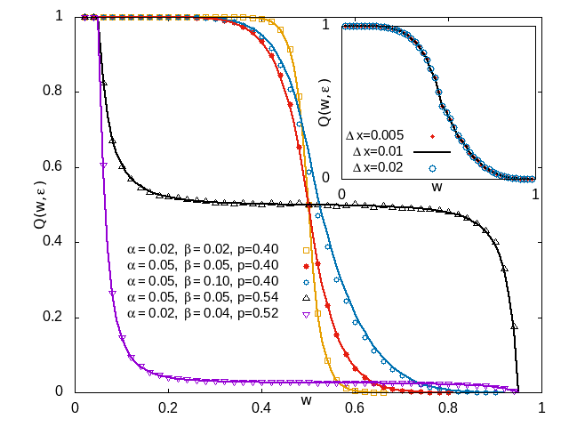
Figure 9: For RDS (69)$Q(w,\epsilon)$ obtained from numerical simulations (symbol) for different $\alpha,\beta$ are compared with the same obtained in (100) using perturbation theory (lines). To obtain $Q(w,\epsilon)$ from simulations, we consider the initial density distributed uniformly in $(w-\Delta x,w+\Delta x)$ with a small $\Delta x.$ The insest shows $Q(w,\epsilon)$ for different $\Delta x.$ Here $\epsilon=0.05.$

For general $\alpha\neq\beta$ we obtain $Q(w,\epsilon)$ from numerical simulations of the model for $\epsilon=0.05$ and compared it with the same obtained in Eq. (100) using a second order approximation. This is shown in Fig. 9; for small $\alpha,\beta,$ the data obtained from simulations (symbols) agree quite well with Eq. (100) (line). But for larger $\alpha,\beta,$ as seen in Fig. 10 , the data differs quite a bit from Eq. (100).

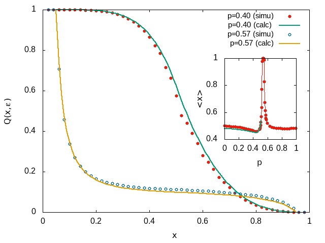
Figure 10: $Q(x,\epsilon)$ versus $x$ for RDS (69) with $\alpha=0.1,\beta=0.2,\epsilon=0.05,p=0.40,0.57,$ obtained from simulations (symbols), are compared with Eq. (100). The inset compares $\langle x\rangle$ versus $p$ in the region where ACIM does not exist -here $\langle x\rangle=1-A$ can be calculated from $Q(x,\epsilon).$ A slight mismatch of $\langle x\rangle,$ simulations (symbol) versus analytical calculations (line), due to the second order approximation that we used for calculating $Q(x,\epsilon).$

We must mention the following crucial point about the numerical simulation. The initial distribution cannot be taken as $\rho_{0}(x)=\delta(x-w)$ as it is not a measurable density. One must take $\rho_{0}(x)$ as a narrow distribution around $x=w,$ say $U(w-\Delta,w+\Delta),$ and calculate $Q(w,\epsilon)$ and then take $\Delta\to 0$ limit. In the inset of Fig. 9, we show $Q(w,\epsilon)$ for three different values of $\Delta=0.02,0.01,0.005;$ the curves are indistinguishable from each other and we consider the smallest $\Delta=0.005$ to obtain $Q(w,\epsilon)$ shown in Figs. 9 and 10.

Note, that $Q(w,\epsilon)$ gives us information about $\langle x\rangle=1-A,$ where $A$ is given in Eq. (94). We calculate $\langle x\rangle$ from simulations for $\alpha=0.1,\beta=0.2,\epsilon=0.05$ and plot it against $p$ (as symbols) in the inset of Fig. 10. The solid line is the value of $1-A$ calculated using Eqs. (94) and (100) which agree reasonably well with the data. This method of calculating $\langle x\rangle$ is valid only when ACIM does not exist and $\rho(x)=A\delta(x)+(1-A)\delta(x-1)$. This explains why $\langle x\rangle$ does not extended beyond $p^{*}$.

V Other Cases

In this section we discuss random maps with features which are not already discussed in the previous sections. In generic RDS, a unique measurable steady state density function does not exist and any definite statement is not feasible. We consider the following specific cases to demonstrate the necessity of a common fixed point and to show why at least one of the common fixed points has to be attractive.

Many common fixed points:

Let us assume that the RDS is bounded in the interval $(0,1)$ and it has $N>2$ common fixed points $\{a_{i}\},$ each one being attractive for at least one of the constituting maps. Without loss of generality we can assume $0\leq a_{1}<a_{2}<\dots<a_{N}\leq 1$. According to the fixed point conjecture, in absence of ACIM we expect $\rho(x)=\sum_{i=1}^{N}A_{i}\delta(x-a_{i})$ and $\sum_{i=1}^{N}A_{i}=1.$ Now we set a small positive parameter $\epsilon$ and force the evolution of the RDS to stop whenever $|x_{t}-a_{i}|<\epsilon$ for any $t.$ Let $Q_{i}(w,\epsilon)$ be the probability that starting from $x_{0}=w,$ the evolution stops near the fixed point $a_{i}.$ Clearly, $\sum_{i=1}^{N}Q_{i}(w,\epsilon)=1.$ Thus, for an initial distribution $\rho(x),$

$$A_{i}=\lim_{\epsilon\to 0}\int_{0}^{a_{i}-\epsilon}dwQ_{i}(w,\epsilon)\rho_{0}(w)+\int_{a_{1}+\epsilon}^{1}dwQ_{i}(w,\epsilon)\rho_{0}(w).$$ (104)

There is no particular difficulty in calculating $A_{i},$ exactly or perturbatively. We skip the details to avoid repetition.

One interesting situation is when the constituting maps are of the following type: for any starting position $a_{i}\leq x_{0}=w\leq a_{i+1},$ $x_{t}$ for any $t$ remains bounded in the interval $(a_{i},a_{i+1}).$ Then, along with the global density conservation (normalization), the density in each interval $(a_{i},a_{i+1})$ is also conserved. Thus, the RDS in this case is reducible to a set of RDSs, each one bounded in the interval $(a_{i},a_{i+1}).$ One can now utilize the methods developed in the previous section for $N=2$ to obtain the total hitting probabilities $C_{i}$ ( $\bar{C}_{i+1}$), the total probability that the RDS in the interval $(a_{i},a_{i+1}),$ starting from $(a_{i}<x<a_{i+1})$ with weight $\rho_{0}(x),$ hits the boundary $a_{i}$ ($a_{i+1}$) before hitting $a_{i+1}$ ($a_{i}$); they obey

$$C_{i}+\bar{C}_{i+1}=\int_{a_{i}}^{a_{i+1}}dx\rho_{0}(x);~{}~{}i=1,2,\dots,N-1$$ (105)

Finally, the weights of the $\delta$-functions $\{C_{i}\}$ are,

$$A_{1}=C_{1},A_{L}=C_{L}~{}{\rm and}~{}A_{i}=C_{i}+\bar{C}_{i}~{}{\rm for}~{}i=2,3,\dots,N-1$$

No common fixed points:

Are common fixed points really necessary? What happens, when the RDS has no fixed points or no common fixed points ? The best case scenario is an RDS, where one of the constituting maps has an attractive fixed point but it is not a common fixed point. In such cases, it is plausible to ask what happens to the steady state density in regions of the parameter space where we do no expect an invariant measure.

Let us consider an example, a RDS with $K=2$:

$$x_{t+1}=\begin{cases}f_{1}(x_{t})=1-|1-2x_{t}|&\text{prob}~{}p\\ f_{2}(x_{t})=1-\frac{3}{4}x_{t}&\text{prob}~{}1-p\end{cases}$$ (106)

Clearly $f_{1}(.)$ has an unstable fixed point at $x=\frac{2}{3}$ and $f_{2}(.)$ has a stable fixed point at $x=\frac{4}{7};$ the RDS has no common fixed point. The Pelikan condition says that the ACIM exists for $p>p^{*}=\frac{2}{5}$. Now we look at the proposition by Yu, Ott and Chen 19 . The Lyapunov exponents of $f_{1,2}(.)$ are $\Lambda=\ln(2)$, and $\ln(\frac{3}{4})$ respectively. Thus the average Lyapunov exponent near the fixed point $x=0$ is positive when $p>p_{\Lambda}=\ln(4/3)/\ln(8/3)\simeq 0.2933$ and we expect a well-defined normalizable density $\rho(x)$ for $p>p_{\Lambda},$ although it may not be measurable at some points. The region of interest is then $p<p_{\Lambda}.$ In this regime, since the average Lyapunov exponent is negative one would expect some localized density 19 . On the other hand, the fixed point conjecture that we propose leads to localized density functions only when there are CFPs. To understand this regime better, we simulate the RDS for $p=0.2,$ which is shown in Fig. 11.

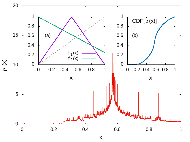
Figure 11: $\rho(x)$ for the RDS (106) which does not have any CFP. The constituting maps are shown in (a). (b) shows the steady state CDF. For $p=0.2,$ ACIM does not exist but the RDS is not attracted to $x=\frac{2}{3},$ an attractive fixed point of the tent-map.

As can be seen in the Fig. 11, the system does not seem to localize. The distribution is measured by taking a bin-size $2^{-16}$ and $10^{9}$ samples where the initial density is uniformly distributed in $(0,1).$ Countable number of $\delta$-like peaks are observed along with a background density which is stationary and finite. The $\delta$-like peaks originate from the fact that the system tries to aggregate at the stable fixed point $\frac{4}{7},$ but it can escape from this neighbourhood using $f_{1}(x)$ with probability $p,$ resulting in additional peaks at $f_{1}(\frac{4}{7}),f_{1}(f_{1}(\frac{4}{7})),f_{2}(f_{1}(4/7)),\dots$ etc. The cumulative density function (CDF) for $\rho(x)$ is shown in the right inset of Fig. 11. The CDF looks continuous, although it exhibits kinks where there are $\delta$-like peaks. This indicates that we have a measurable density $\rho(x)$ at $p=0.2<p_{\Lambda}<p^{*}.$ This highlights the necessity of a CFP for the localization transition. This example also indicates that the criteria by Pelikan Pelikan and by Ott and Chen 19 are only sufficient conditions.

We must mention another interesting example considered in boss , where the dynamics of a random walk in a bounded domain has been mapped to an RDS, consisting of four different functions in a simple set up. They considered a two dimensional random walk $(x,y)_{t+1}=(x,y)_{t}+(\sigma_{x},\sigma_{y})$ where $\sigma_{x,y}=\pm 1$ is a stochastic variable; when the walker crosses the boundary it comes back deterministically to a predefined base curve and starts walking again. In effect, one point on the base-curve is mapped to another point by a random map, which is a random path that crosses the boundary. The distribution of returning walkers on the base-curve was found to be not well-defined; the signature of this was found in corresponding CDF, which turned out to be a Devil’s staircase. In these maps, clearly the Pelikan condition is invalid and the RDS does not have any CFP.

VI Summary

In this article we have investigated the possible steady states that random dynamical systems (RDS) or random maps lead to. In contrast to stochastic maps, where a discrete time deterministic evolution is influenced by an additive noise, in random maps the mapping functions are chosen with certain probability from a given set of functions. Naturally, RDS makes the evolving variable $x_{t}$ a stochastic variable and brings in a possibility of having a stationary distribution $\rho(x)$ in the thermodynamic limit $t\to\infty.$ Surprisingly, generic random maps consisting of any arbitrary bounded functions do not always lead to a unique and measurable steady state density. A sufficient condition on constituting functions for having an absolutely continuous invariant measure (ACIM) was derived by Pelikan in 1984 Pelikan . We explored the region where Pelikan’s criterion breaks down and have obtained additional specifications which may help us infer the nature of the steady state.

The existence of ACIM usually refers to having a steady state with well-defined probability density $\rho(x)$. In regions where nothing can be inferred about the ACIM from the Pelikan condition, the steady state density, $\rho(x)$ may still exist and diverge at some $x$ but is still normalizable. This, we show through many examples of Markov maps. For Markov maps, where the RDS on a bounded domain $I$ can be mapped to a Markov process on some suitable sub-intervals $\{I_{i}\}$ of width $\{w_{i}\},$ this normalizability condition translates to $\sum_{i}c_{i}w_{i}=1$ where the steady state weights $\{c_{i}\}$ may diverge in some sub-interval(s). We have demonstrated this using exact steady state results for a specific RDS with three mapping functions. Ott and Chen 19 have proposed an interesting criterion based on the Lyapunov exponents of the constituting maps that captures both the regions, where ACIM exists and where $\rho(x)$ normalizable and the Pelikan criterion does not predict anything; the average Lyapunov exponent must be positive in these regions. Beyond these regions $\rho(x)$ may not be unique or well-defined. Here, the fixed point conjecture that we propose provide an insight about the steady states.

We conjecture that when the RDS has a set of $N$ common fixed points (CFPs) at $\{x=a_{i}\}$ each being stable for at least one of the constituting maps, then $\rho(x)=\sum_{i}C_{i}\delta(x-a_{i});$ the weights $A_{i}$ are not unique as they depend on the initial density $\rho_{0}(x).$ For $N=1,$ trivially $C_{1}=1.$ For $N=2,$ we show that weights $C_{1}$ and $C_{2}$ can be considered as the probability that a one-dimensional random walker hits one of the boundaries before hitting the other – of course the random walk is not a simple one-step walk on a lattice. This mapping helps us get the weights exactly for several maps. We also provide a perturbative approach to derive it when exact analytical solutions are not possible.

We believe that non-existence of a well-defined density function is the generic feature of random maps which have no CFPs. Both Pelikan’s criterionPelikan and the criteria by Ott and Chen 19 are only sufficient conditions for having a well-defined density function. When they fail, $\rho(x)$ is localized at the CFPs which are attractive for at least one of the constituting maps. In absence of CFPs, $\rho(x)$ may not exist at all, or it may exist along with a countable set of $\delta$ functions, like we see in Eq. (106).

Although random dynamical systems have been a subject of research interest in mathematics for for long, it has been finding applications recently in modelling climate 24 , synchronization sync , on-off intermittency inter , path coalescence 21 , and anomalous diffusion Sato2019 ; 20 . We sincerely hope that this article would bring in new and interesting directions of research and applications.

- (1) R. Kautz, Chaos: The Science of Predictable Random Motion, Oxford University Press, Oxford(2011).
- (2) L. Arnold, Random Dynamical Systems, Springer Monographs in Mathematics (Corrected 2nd Printing, 2003).
- (3) S. Pelikan, Trans. Amer. Math. Soc. 281, 813 (1984).
- (4) L. Yu, E. Ott, and Q. Chen, Phys. Rev. Lett. 65, 2935 (1990).
- (5) M. Majumdar and R. Bhattacharya, Random Dynamical Systems: Theory and Applications, Cambridge University Press, London (2007).
- (6) A. Boyarsky and P. Góra, Laws of chaos: invariant measures and dynamical systems in one dimension. (Springer Science & Business Media, 2012)
- (7) A. Lipowski, I. Bena, M. Droz and A.L. Ferreira, Physica A 339, 237 (2004).
- (8) T. Bódai, E. Altmann, and A. Endler, Phys. Rev. E. 87, 042902 (2013).
- (9) P. W. Hammer, N. Platt, S. M. Hammel, J. F. Heagy, and B. D. Lee, Phys. Rev. Lett. 73, 1095 (1994).
- (10) M. Chekroun, E. Simonnet, and M. Ghil, Physica D 240, 1685 (2011).
- (11) M. Ghil, V. Lucarini, Rev. Mod. Phys. 92, 35002 (2020).
- (12) Anatoliy Swishchuk, Shafiqul Islam, Random Dynamical Systems in Finance, CRC Press, Taylor & Francis Group, New York (2013).
- (13) Y. Sato and R. Klages, Phys. Rev. Lett. 122, 174101 (2019)
- (14) M. Wilkinson, B. Mehlig, K. Gustavsson, and E. Werner, Eur. Phys. J. B 85, 18 (2012).
- (15) M. Wilkinson and B. Mehlig, Phys. Rev. E 68, 040101(R) (2003).
- (16) P. Góra and A. Boyarsky, J. Math. Anal. Appl. 278, 225 (2003).
- (17) A. Boyarsky and Y. S. Lou, Dyn. and Stab. of Sys. 7, 233 (1992).
- (18) W. Bahsoun and P. Góra, Stud. Math. 166, 271 (2005).
- (19) M. Islam, P. Góra, and A. Boyarsky, J. Appl. Math. Stoch. Anal. 2, 133 (2005).
- (20) G. Froyland, Nonlinearity 12, 1029 (1999).
- (21) M. Islam, Int. J. Bif. Chaos. 23, 1350025 (2013).
- (22) T. Inoue, Stud. Math. 208, 11 (2012).
- (23) A. Lasota and J. Yorke,Trans. Am. Math. Soc. 186, 481 (1973).
- (24) R. Bowen, Commun. Math. Phys. 69, 1 (1979).
- (25) W. Feller, An Introduction to Probability Theory and Its Applications 3rd Ed., Wiley (1970).
- (26) M. Basu and P. K. Mohanty, EPL 90, 50005 (2010)