Sparsity-Aware SSAF Algorithm with Individual Weighting Factors for Acoustic Echo Cancellation

Abstract

In this paper, we propose and analyze the sparsity-aware sign subband adaptive filtering with individual weighting factors (S-IWF-SSAF) algorithm, and consider its application in acoustic echo cancellation (AEC). Furthermore, we design a joint optimization scheme of the step-size and the sparsity penalty parameter to enhance the S-IWF-SSAF performance in terms of convergence rate and steady-state error. A theoretical analysis shows that the S-IWF-SSAF algorithm outperforms the previous sign subband adaptive filtering with individual weighting factors (IWF-SSAF) algorithm in sparse scenarios. In particular, compared with the existing analysis on the IWF-SSAF algorithm, the proposed analysis does not require the assumptions of large number of subbands, long adaptive filter, and paraunitary analysis filter bank, and matches well the simulated results. Simulations in both system identification and AEC situations have demonstrated our theoretical analysis and the effectiveness of the proposed algorithms.

I Introduction

Adaptive filtering algorithms have been extensively developed in Gaussian noise environments [1, 2], and representative examples are the least mean square (LMS) and normalized LMS (NLMS) algorithms. However, impulsive noise is often encountered in realistic environments such as echo cancellation, underwater acoustics, audio processing, communications, and prediction of time-series [3, 4, 5, 6, 7, 8]. Although the impulsive noise appears randomly with a small probability or a short duration, its realizations have large amplitude. In this situation, the algorithms based on Gaussian noise suffer from a poor convergence or even divergence. Aiming at impulsive noise, Mathews et al. first proposed the sign algorithm which minimizes the absolute value of the error signal [9]. The maximum correntropy criterion was frequently studied to present efficient and robust LMS-like algorithms in impulsive noise [10, 11, 12], thanks mainly to the strong compression capability of the correntropy function on the error signals with large amplitude.

The problem of the aforementioned algorithms is the slow convergence when the input signal to the adaptive filter is highly correlated. To speed up the convergence, the subband adaptive filter (SAF) is one of the promising approaches [2]. In the SAF, the input signal is divided into multiple subband components through the analysis filters, and then the decimated subband input signals that have approximately uncorrelated samples are used for updating the filter’s weights. Among the SAF’s structures, its multiband structure updates the fullband-like filter’s weights is more promising due to avoiding the aliasing and band edge effects [2]. Based on the multiband structure, the normalized SAF (NSAF) algorithm in [13] converges faster than the NLMS algorithm for highly correlated inputs. The excess computational complexity of the NSAF over the NLMS is trivial, especially for long filter applications such as echo cancellation. By incorporating the sign algorithm into the SAF, the sign subband adaptive filter (SSAF) algorithm was proposed in [14], with good robustness against impulsive noise. By fully taking advantage of the decorrelation feature of SAF, the individual-weighting-factors based SSAF (IWF-SSAF) algorithm [15] provides faster convergence than the SSAF algorithm. Note that, when users choose the fixed step-size, both SSAF algorithms need to consider a trade-off between fast convergence and low steady-state error. To address this problem, several variable step-size (VSS) strategies were developed for both algorithms that drive fast convergence and low steady-state error simultaneously, to name a few, the VSS-SSAF [16] and band-dependent VSS SSAF (BDVSS-SSAF) [17] algorithms from the mean-square deviation (MSD) minimization, and the novel VSS SSAF [18] and band-dependent VSS IWF-SSAF (BDVSS-IWF-SSAF) [19] algorithms based on the $l_{1}$-norm minimization, and the robust VSS SSAF algorithm [20]. Among them, the VSS strategies in [18] and [19] do not require the a priori knowledge of the surrounding noise, e.g., the noise variance and the occurrence probability of impulsive noise. The performance analysis is always a vital research issue for adaptive filtering algorithms [1, 21, 22, 23, 24, 25]. It is beneficial to support the effectiveness of a specific adaptive filtering algorithm in theory and to give useful insights to further improve the adaptive filter’s performance. It is worth noting that one often pays attention to the performance analyses of adaptive filtering algorithms in Gaussian noise surroundings. For example, there have been different analysis models on the MSD behavior of the NSAF algorithm [26, 27, 28, 29]. Relatively speaking, it is more difficult to analyze the performance of robust adaptive filtering algorithms in impulsive noise. In [30], the steady-state MSD of the SSAF algorithm in impulsive noise was analyzed based on the energy conservation relation, and in [15] the same analysis pattern was also extended to the IWF-SSAF algorithm. However, this analysis approach relies on the assumptions of large number of subbands and long adaptive filter. By assuming the background noise to be Gaussian, the analytical expression in [31] shows better accuracy than the one in [30] for the steady-state MSD of the SSAF algorithm. Nevertheless, the advantage of the SSAF algorithm is working in impulsive noise, so in this case the analysis in [31] is not applicable.

On the other hand, the aforementioned algorithms have not exploited the underlying sparsity of the systems. Sparse systems are common in practice, with the property that its impulse response only has a few large non-zero coefficients (active coefficients) and the remaining coefficients are zero or approach zero (inactive coefficients), such as network/acoustic echo channels [32, 33], underwater acoustic channels [34], and digital TV transmission channels [35]. In order to favor such sparsity, the sparsity-aware technique is popular in adaptive filtering algorithms [36, 37, 38, 39] that adds the sparse constraint term in the original cost function. In the survey of robust SAF against impulsive noise, sparsity-aware approaches were only incorporated straightforwardly into the SSAF  [40] and normalized logarithmic SAF [41] algorithms, and have not been analyzed theoretically yet. Also, the resulting algorithms require properly choosing the sparsity penalty parameter in a trial and error way, thereby limiting their usefulness.

It is remarked that the acoustic echo cancellation (AEC) application involves the above-mentioned three characteristics: high correlation of speech input signals, double-talk that is one type of impulsive noise scenarios, and sparsity of acoustic echo channels. For the sake of these requirements, therefore, this paper will focus on studying the sparsity-aware IWF-SSAF (S-IWF-SSAF) algorithm. Our main contributions are as follows:

1) By incorporating the sparsity-aware technique, we propose the S-IWF-SSAF algorithm, and analyze its performance in-depth in impulsive noise. The analysis result reveals that S-IWF-SSAF can be superior to IWF-SSAF in sparse system environments, but it requires properly choosing the sparsity penalty parameter in a certain range.

2) The proposed analysis covers the behaviors of the IWF-SSAF algorithm in impulsive noise. Even though for the IWF-SSAF algorithm, the proposed analysis is significantly more accurate than the analysis in [15] and closely matches the simulations, because it obviates the assumptions of a large number of subbands, long adaptive filter, and paraunitary analysis filter bank.

3) We devise a joint optimization scheme to automatically choose the step-size and the sparsity penalty parameter, which further improves the convergence and steady-state performance of the S-IWF-SSAF algorithm.

4) In order to make the proposed algorithms suitable for AEC, we develop delayless implementation of the proposed algorithms and carry out a simulation study.

The notations used in this paper are listed in Table 1. This paper is organized as follows. In Section 2, we state the SAF problem of interest and briefly review the IWF-SSAF algorithm. Then, we propose the S-IWF-SSAF algorithm in Section 3 and analyze its performance in Section 4. In Section 5, the VSS mechanism and the variable sparsity penalty parameter for the S-IWF-SSAF algorithm are devised. In Section 6, simulation results in both system identification and AEC scenarios are presented. Finally, conclusions are given in Section 7.

TABLE I: Some Mathematical Symbols.

Notations	Description
$(\cdot)^{\text{T}}$	transpose of a vector or matrix
$||\cdot||_{2}$	$l_{2}$-norm of a vector
$\text{sgn}(\cdot)$	sign function
$\text{E}\{\cdot\}$	expectation of a random variable
$\text{Tr}(\cdot)$	trace of a matrix
$\text{vec}(\cdot)$	yielding an $L^{2}\times 1$ vector from an $L\times L$ matrix by successively stacking the columns of the matrix
$\text{vec}^{-1}(\cdot)$	the inverse operation of $\text{vec}(\cdot)$
$\otimes$	Kronecker product of two matrices

II Problem Statement and The IWF-SSAF Algorithm

Let us consider a system identification problem that identifies the impulse response of the unknown system, denoted as an $M$-length column vector. By feeding the input signal $u(n)$ into the unknown system, the desired signal $d(n)$ of the system at discrete time $n$ is formulated as

$$d(n)=\bm{u}^{\text{T}}(n)\bm{w}^{o}+v(n)$$ (1)

where $\bm{u}(n)=[u(n),u(n-1),...,u(n-M+1)]^{\text{T}}$ is the $M\times 1$ input vector, and $v(n)$ denotes the additive noise.

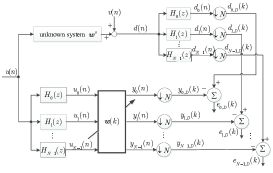
Figure 1: Multiband structure of SAF.

Fig. 1 shows the multiband structure of SAF with $N$ subbands [2]. The desired signal $d(n)$ and the input signal $u(n)$ are decomposed into multiple subband signals $d_{i}(n)$ and $u_{i}(n)$, respectively, through the analysis filter bank $\{H_{i}(z)\}_{i=0}^{N-1}$. Then, for each band $i$, the signal $u_{i}(n)$ is filtered by the common filter (whose weight vector is $\bm{w}(k)$) to get the output signal $y_{i}(n)$. By critically decimating sequences $d_{i}(n)$ and $y_{i}(n)$, respectively we obtain lower sampled-rate sequences $d_{i,D}(k)$ and $y_{i,D}(k)$, namely, $d_{i,D}(k)=d_{i}(kN)$ and $y_{i,D}(k)=\bm{u}^{\text{T}}_{i}(k)\bm{w}(k)$, where $\bm{u}_{i}(k)=[u_{i}(kN),u_{i}(kN),...,u_{i}(kN-M+1)]^{\text{T}}$. By subtracting $y_{i,D}(k)$ from $d_{i,D}(k)$ for $i=0,...,N-1$, the decimated subband error signals used for updating $\bm{w}(k)$ are obtained:

$$\begin{array}[]{rcl}\begin{aligned} e_{i,D}(k)=d_{i,D}(k)-\bm{u}^{\text{T}}_{i}(k)\bm{w}(k).\end{aligned}\end{array}$$ (2)

Since $\bm{w}(k)$ is an estimate of $\bm{w}^{o}$ in the decimated domain $k$, the main task of the adaptive filter is how to adjust $\bm{w}(k)$ by using the available signals $\{d_{i,D}(k),u_{i}(k),e_{i,D}(k)\}_{i=0}^{N-1}$ to reach quickly $\bm{w}(k)\rightarrow\bm{w}^{o}$ as $k$ increases.

To estimate $\bm{w}^{o}$ in impulsive noise, the cost function with the band-dependent weighting factor $\lambda_{i}$ is defined as

$$J(k)=\sum\limits_{i=0}^{N-1}\zeta_{i}|e_{i,D}(k)|.$$ (3)

By applying the instantaneous gradient descent (IGD) principle to minimize (3) with respect to $\bm{w}(k)$ and letting $\zeta_{i}=1/\|\bm{u}_{i}(k)\|_{2}$, the weight vector of the IWF-SSAF algorithm is recursively updated [15]:

$$\bm{w}(k+1)=\bm{w}(k)+\mu\sum\limits_{i=0}^{N-1}\frac{\text{sgn}(e_{i,D}(k))\bm{u}_{i}(k)}{\|\bm{u}_{i}(k)\|_{2}}$$ (4)

where $\mu>0$ is the step-size. Due to the sign function $\text{sgn}(\cdot)$, the IWF-SSAF algorithm is robust against impulsive noise.

III Proposed S-IWF-SSAF algorithm

Based on sparsity-aware techniques [36, 37, 38, 39, 42], we modify the cost function in (3) as

$$J_{s}(k)=\sum\limits_{i=0}^{N-1}\zeta_{i}|e_{i,D}(k)|+\rho H(\bm{w}),$$ (5)

where $H(\bm{w})$ is the penalty term for favoring the sparsity of $\bm{w}^{o}$, and $\rho>0$ is the sparsity penalty parameter associated with this term. By applying the IGD principle to reach a minimization of (5), the proposed S-IWF-SSAF algorithm for updating the weight vector is formulated as

$$\bm{w}(k+1)=\bm{w}(k)+\mu\sum\limits_{i=0}^{N-1}\frac{\text{sgn}(e_{i,D}(k))\bm{u}_{i}(k)}{\|\bm{u}_{i}(k)\|_{2}}-\rho H^{\prime}(\bm{w}(k)),$$ (6)

where $H^{\prime}(\bm{w})\triangleq\frac{\partial H(\bm{w})}{\partial\bm{w}}$ is the subgradient of $H^{\prime}(\bm{w})$ with respect to $\bm{w}$, and here the parameter $\rho$ has absorbed $\mu$. Furthermore, (6) can be implemented equivalently by two steps:

$$\bm{\varphi}(k+1) =\bm{w}(k)+\mu\sum\limits_{i=0}^{N-1}\frac{\text{sgn}(e_{i,D}(k))\bm{u}_{i}(k)}{\|\bm{u}_{i}(k)\|_{2}},$$ (7a)

$$\bm{w}(k+1) =\bm{\varphi}(k+1)-\rho H^{\prime}(\bm{\varphi}(k+1)).$$ (7b)

In equation (7), the first step plays the adaptive learning role of the IWF-SSAF algorithm, and the second step drives inactive coefficients in $\bm{\varphi}(k+1)$ to zero to further improve the estimation performance of $\bm{w}^{o}$. Note that, in (7b) we have also made a replacement of $H^{\prime}(\bm{w}(k))$ with $H^{\prime}(\bm{\varphi}(k+1))$. By doing so, we are able to relatively independently design the adaptive choices of $\mu$ and $\rho$ according to (7a) and (7b), respectively, which will be discussed in the sequel. Now, another issue is the choice of the penalty term $H(\bm{w})$. In the literature, several strategies on $H(\bm{w})$ have been reported to present different sparsity-aware adaptive filtering algorithms, see [42, 37, 38] and references therein. Here, we do not discuss the effect of these strategies, and choose the popular log-penalty:

$$H(\bm{\varphi}(k+1))=\sum_{m=1}^{M}\ln(1+|\varphi_{m}(k+1)|/\xi),$$ (8)

where $\varphi_{m}(k+1)$ denotes the $m$-th entry of $\bm{\varphi}(k+1)$, and $\xi>0$ denotes the shrinkage magnitude that distinguish active entries and inactive entries. Accordingly, $H^{\prime}(\bm{\varphi}(k+1))$ in (7b) is given by

$$H^{\prime}(\varphi_{m}(k+1))=\frac{\text{sgn}(\varphi_{m}(k+1))}{\xi+|\varphi_{m}(k+1)|},m=1,...,M.$$ (9)

We note that the proposed algorithms can also be considered in the context of detection problems [43, 44, 45, 46, 47, 48, 49, 50, 51, 52, 53, 54, 55, 56, 57, 58, 59, 60, 61, 62, 64, 65, 66, 63, 67] and might be further enhanced by exploitation of low-rank techniques [68, 69, 70, 71, 72, 73, 74, 75, 76, 77, 78, 79, 80, 81, 82, 83, 84, 85, 86, 87, 88, 89, 90, 91, 92, 93, 94, 95, 96, 97, 98, 99, 100, 101, stapcoprime, 102, 103, 104].

IV Performance Analysis

In this section, we study in detail the statistical performance of the S-IWF-SSAF algorithm in the presence of impulsive noise, and in theory illustrate its superiority over the IWF-SSAF algorithm when identifying sparse systems.

Assuming that $\bm{w}^{o}$ is time-invariant. Then, from (7a) and (7b) we obtain the following weights error vector recursions:

$$\widetilde{\bm{\varphi}}(k+1) =\widetilde{\bm{w}}(k)-\mu\sum\limits_{i=0}^{N-1}\frac{\text{sgn}(e_{i,D}(k))\bm{u}_{i}(k)}{\|\bm{u}_{i}(k)\|_{2}},$$ (10a)

$$\widetilde{\bm{w}}(k+1) =\widetilde{\bm{\varphi}}(k+1)+\rho H^{\prime}(\bm{\varphi}(k+1)),$$ (10b)

where $\widetilde{\bm{w}}(k)\triangleq\bm{w}^{o}-\bm{w}(k)$ and $\widetilde{\bm{\varphi}}(k)\triangleq\bm{w}^{o}-\bm{\varphi}(k)$.

Let $\{\bm{h}_{i}\}_{i=0}^{N-1}$ be the impulse response of the analysis filter bank $\{H_{i}(z)\}_{i=0}^{N-1}$, with the length of $L$, then the following relations hold:

$$\begin{array}[]{rcl}\begin{aligned} \bm{u}_{i}(k)&=[\bm{u}(kN),...,\bm{u}(kN-L+1)]\bm{h}_{i}\\ v_{i,D}(k)&=\bm{h}_{i}^{\text{T}}[v(kN),...,v(kN-L+1)]^{\text{T}}.\end{aligned}\end{array}$$ (11)

Therefore, (2) can be rearranged as

$$\begin{array}[]{rcl}\begin{aligned} e_{i,D}(k)=e_{i,a}(k)+v_{i,D}(k),\end{aligned}\end{array}$$ (12)

where $e_{i,a}(k)\triangleq\bm{u}^{\text{T}}_{i}(k)\widetilde{\bm{w}}(k)$ denotes the a priori subband error. Equations (10)-(12) will be the starting point to study the mean and mean-square behaviors of the algorithm in the sequel. Moreover, in order to help to analyze the algorithm mathematically, some widely used assumptions are made as follows:

Assumption 1: The input vector $\bm{u}(n)$ is random with zero-mean vector and positive definite autocorrelation matrix $\bm{R}_{u}=\text{E}\{\bm{u}(n)\bm{u}^{\text{T}}(n)\}$.

Assumption 2: The additive noise $v(n)$ is drawn from the contaminated-Gaussian (CG) process, i.e., $v(n)=v_{\text{g}}(n)+v_{\text{im}}(n)$. Specifically, the background noise $v_{\text{g}}(n)$ is white Gaussian with zero-mean and variance $\sigma_{\text{g}}^{2}$. The impulsive noise component $v_{\text{im}}(n)$ is described by the Bernoulli-Gaussian model $v_{\text{im}}(n)=b(n)\eta(n)$, where $b(n)$ obeys the Bernoulli distribution that the probability of occurring 1 is $P\{b(n)=1\}=p_{r}$, and $\eta(n)$ is also zero-mean white Gaussian but with variance $\sigma_{\eta}^{2}=\hbar\sigma_{\text{g}}^{2}$, $\hbar\gg 1$. Thus, it is seen that $v(n)$ is non-Gaussian for any $p_{r}$ excluding two special cases $p_{r}=0$ and 1 [105]

Assumption 3: $\widetilde{\bm{w}}(k)$ is independent of $\bm{u}_{i}(k)$ for $i=0,...,N-1$.

Note that, with the relation (11), assumption 1 shows that the $i$-th subband’s input vector $\bm{u}_{i}(k)$ is also zero-mean and has a positive definite autocorrelation matrix $\bm{R}_{i}=\text{E}\{\bm{u}_{i}(k)\bm{u}_{i}^{\text{T}}(k)\}$. Assumption 2 is a popular model for analyzing the performance of adaptive filtering algorithms in impulsive noise [42, 105]. Assumption 3 is the well-known independence assumption for the performance analysis of adaptive filtering algorithms [1, 106].

IV-A Mean behavior

By imposing the expectations on both sides of (10a) and (10b), we have

$$\text{E}\{\widetilde{\bm{\varphi}}(k+1)\} =\left(\bm{I}_{M}-\mu\sum\limits_{i=0}^{N-1}\Omega_{i}(k)\text{E}\{\bm{A}_{i}(k)\}\right)\text{E}\{\widetilde{\bm{w}}(k)\},$$ (13a)

$$\text{E}\{\widetilde{\bm{w}}(k+1)\} =\text{E}\{\widetilde{\bm{\varphi}}(k+1)\}+\rho\text{E}\{H^{\prime}(\bm{\varphi}(k+1))\},$$ (13b)

where

$$\Omega_{i}(k)=\sqrt{\frac{2}{\pi}}\left[\frac{p_{r}}{\sqrt{\text{E}\{e_{i,D,1}^{2}(k)\}}}+\frac{1-p_{r}}{\sqrt{\text{E}\{e_{i,D,2}^{2}(k)\}}}\right]\neq 0,$$ (14)

$$\text{E}\{e_{i,D,1}^{2}(k)\}=\text{E}\{e_{i,a}^{2}(k)\}+||\bm{h}_{i}||_{2}^{2}(\hbar+1)\sigma_{\text{g}}^{2},$$ (15)

and

$$\text{E}\{e_{i,D,2}^{2}(k)\}=\text{E}\{e_{i,a}^{2}(k)\}+||\bm{h}_{i}||_{2}^{2}\sigma_{\text{g}}^{2}.$$ (16)

Note that, the detailed process of (13a) is shown in Appendix A. Supposing that the algorithm converges, it holds that $\text{E}\{\widetilde{\bm{w}}(k+1)\}=\text{E}\{\widetilde{\bm{w}}(k)\}$ as $k\rightarrow\infty$. Hence, from (13a) and (13a) we can deduce the following theorem.

Theorem 1.

When $k\rightarrow\infty$, it is established that

$$\text{E}\{\widetilde{\bm{w}}(\infty)\} =\frac{\rho}{\mu}\left(\sum\limits_{i=0}^{N-1}\Omega_{i}(\infty)\text{E}\{\bm{A}_{i}(\infty)\}\right)^{-1}\text{E}\{H^{\prime}(\bm{w}(\infty))\},$$ (17)

which points out that the S-IWF-SSAF algorithm is biased for estimating a sparse vector $\bm{w}^{o}$.

Remark 1: For a special case of $\rho=0$, (17) leads to

$$\text{E}\{\widetilde{\bm{w}}(\infty)\}=\bm{0},$$ (18)

that is, the IWF-SSAF algorithm is unbiased for estimating $\bm{w}^{o}$ in the presence of impulsive noise.

It is worth noting that the mean transient behavior of both IWF-SSAF and S-IWF-SSAF algorithms relies on its mean-square behavior as we shall discuss below.

IV-B Mean-square behavior

Let us define the autocorrelation matrices of the weight error vectors $\widetilde{\bm{w}}(k)$ and $\widetilde{\bm{\varphi}}(k)$, as follows, $\widetilde{\bm{W}}(k)\triangleq\text{E}\{\widetilde{\bm{w}}(k)\widetilde{\bm{w}}^{\text{T}}(k)\}$ and $\widetilde{\bm{\varPhi}}(k)\triangleq\text{E}\{\widetilde{\bm{\varphi}}(k)\widetilde{\bm{\varphi}}^{\text{T}}(k)\}$. Thus, by equating the autocorrelation matrices for both sides of (10a) and (10b) respectively, we have the following recursions:

$$\begin{array}[]{rcl}\begin{aligned} \widetilde{\bm{\varPhi}}(k+1)=&\widetilde{\bm{W}}(k)+\mu^{2}\sum\limits_{i=0}^{N-1}\text{E}\{\check{\bm{A}}_{i}(k)\}-\\ &\mu\widetilde{\bm{W}}(k)\sum\limits_{i=0}^{N-1}\Omega_{i}(k)\text{E}\{\bm{A}_{i}(k)\}-\\ &\mu\sum\limits_{i=0}^{N-1}\Omega_{i}(k)\text{E}\{\bm{A}_{i}(k)\}\widetilde{\bm{W}}(k),\end{aligned}\end{array}$$ (19a)

$$\begin{array}[]{rcl}\begin{aligned} \widetilde{\bm{W}}(k+1)=&\widetilde{\bm{\varPhi}}(k+1)+\rho\bm{\varTheta}(k+1)+\\ &\rho\bm{\varTheta}^{\text{T}}(k+1)+\rho^{2}\bm{\varXi}(k+1),\end{aligned}\end{array}$$ (19b)

where $\bm{\varTheta}(k+1)\triangleq\text{E}\{H^{\prime}(\bm{\varphi}(k+1))\widetilde{\bm{\varphi}}^{\text{T}}(k+1)\}$ and $\bm{\varXi}(k+1)\triangleq\text{E}\{H^{\prime}(\bm{\varphi}(k+1)){H^{\prime}}^{\text{T}}(\bm{\varphi}(k+1))\}$. Note that, the derivation of (19a) is given in Appendix B. Obviously, the mean model in (13b) and the mean-square model in (19b) require computing $\text{E}\{H^{\prime}(\bm{\varphi}(k+1))\}$, $\bm{\varTheta}(k+1)$, and $\bm{\varXi}(k+1)$ beforehand in a component-wise way, as shown in Appendix C. Furthermore, to implement the recursion in (19a) conveniently, $\Omega_{i}(k)$ given by (14) is rewritten as

$$\Omega_{i}(k)= \sqrt{\frac{2}{\pi}}\left[\frac{p_{r}}{\sqrt{\text{Tr}\{\widetilde{\bm{W}}(k)\bm{R}_{i}\}+||\bm{h}_{i}||_{2}^{2}(\hbar+1)\sigma_{\text{g}}^{2}}}+\right.$$ (20)

$$\left.\frac{1-p_{r}}{\sqrt{\text{Tr}\{\widetilde{\bm{W}}(k)\bm{R}_{i}\}+||\bm{h}_{i}||_{2}^{2}\sigma_{\text{g}}^{2}}}\right].$$

The MSD is defined as $\text{MSD}(k)\triangleq\text{E}\{||\widetilde{\bm{w}}(k)||_{2}^{2}\}=\text{Tr}\{\widetilde{\bm{W}}(k)\}$ [1]. Consequently, the model in (19) describes the transient MSD behavior of the S-IWF-SSAF algorithm in impulsive noise.

To continue the steady-state analysis, we impose the vectorization operation on both sides of (19a) and use the Kronecker property that $\text{vec}(\bm{X}\bm{\Sigma}\bm{Y})=(\bm{Y}^{\text{T}}\otimes\bm{X})\text{vec}(\bm{\Sigma})$ for matrices $\bm{X}$, $\bm{Y}$, and $\bm{\Sigma}$ of compatible sizes[107], the following recursion is established:

$$\text{vec}(\widetilde{\bm{\varPhi}}(k+1))=\bm{F}_{k}\text{vec}(\widetilde{\bm{W}}(k))+\mu^{2}\text{vec}\left(\sum\limits_{i=0}^{N-1}\text{E}\{\check{\bm{A}}_{i}(k)\}\right),$$ (21)

where

$$\bm{F}_{k}= \bm{I}_{M^{2}}-\mu\left(\sum\limits_{i=0}^{N-1}\Omega_{i}(k)\text{E}\{\bm{A}_{i}(k)\}\otimes\bm{I}_{M}\right)-$$ (22)

$$\mu\left(\bm{I}_{M}\otimes\sum\limits_{i=0}^{N-1}\Omega_{i}(k)\text{E}\{\bm{A}_{i}(k)\}\right).$$

At the steady-state, it holds that ${\widetilde{\bm{W}}(k+1)}=\widetilde{\bm{W}}(k)$, $k\rightarrow\infty$. Therefore, by assuming the existence of $(\bm{I}_{M^{2}}-\bm{F}_{\infty})^{-1}$ and applying the operators $\text{vec}(\cdot)^{-1}$ and $\text{Tr}(\bm{X}\bm{Y})=\text{vec}^{\text{T}}(\bm{X}^{\text{T}})\text{vec}(\bm{Y})$, the steady-state MSD of the S-IWF-SSAF algorithm can be derived from (19b) and (21) that

$$\begin{array}[]{rcl}\begin{aligned} &\text{MSD}_{s}(\infty)=\text{MSD}(\infty)+\Delta_{s}(\infty),\end{aligned}\end{array}$$ (23)

where

$$\begin{array}[]{rcl}\begin{aligned} &\text{MSD}(\infty)=\\ &\;\mu^{2}\text{vec}^{\text{T}}(\bm{I}_{M})(\bm{I}_{M^{2}}-\bm{F}_{\infty})^{-1}\text{vec}\left(\sum\limits_{i=0}^{N-1}\text{E}\{\check{\bm{A}}_{i}(k)\}\right)\end{aligned}\end{array}$$ (24)

is the result of the IWF-SSAF update (7a) and

$$\begin{array}[]{rcl}\begin{aligned} \Delta_{s}(\infty)=&\text{vec}^{\text{T}}(\bm{I}_{M})(\bm{I}_{M^{2}}-\bm{F}_{\infty})^{-1}\times\\ &\text{vec}\left(\rho\bm{\varTheta}(\infty)+\rho\bm{\varTheta}^{\text{T}}(\infty)+\rho^{2}\bm{\varXi}(\infty)\right)\end{aligned}\end{array}$$ (25)

is the result of the sparsity-aware step (7b).

It is stressed that (23) is not a closed-form, as it is self-contained through $\Omega_{i}(\infty)$. Thus, in terms of $\text{MSD}_{s}(\infty)$, we may take advantage of some numerical approaches to solve (23) or take the MSD value by running (19) to the steady-state. From (23), the following theorem can be obtained.

Theorem 2.

In sparse system scenarios, the steady-state performance of the S-IWF-SSAF algorithm would be superior to that of the IWF-SSAF algorithm, if and only if $\Delta_{s}(\infty)<0$. Interestingly, the possibility of $\Delta_{s}(\infty)<0$ is true by choosing $\rho$ in a range $0<\rho<\rho_{\text{up}}$.

Proof.

See Appendix D. ∎

Remark 2 (on the special IWF-SSAF algorithm): For evaluating the steady-state of the IWF-SSAF algorithm using a small step-size, i.e., (24), it can be assumed that $\text{Tr}(\widetilde{\bm{W}}(\infty)\bm{R}_{i})\ll||\bm{h}_{i}||_{2}^{2}\sigma_{\text{g}}^{2}$. As such, we can make the following approximation for $\Omega_{i}(\infty)$:

$$\Omega_{i}(\infty)\approx\sqrt{\frac{2}{\pi}}\left[\frac{p_{r}}{\sqrt{||\bm{h}_{i}||_{2}^{2}(\hbar+1)\sigma_{\text{g}}^{2}}}+\frac{1-p_{r}}{\sqrt{||\bm{h}_{i}||_{2}^{2}\sigma_{\text{g}}^{2}}}\right],$$ (26)

which contributes a closed-form of $\text{MSD}(\infty)$. On the other hand, when the number of subbands is large enough, the decimated input signal at each subband can be approximately white [2]. Also, the length of the adaptive filter is required to be long. In this case, it is known from [15] that $\text{E}\{\bm{A}_{i}(k)\}\approx\frac{\sigma_{u,i}}{\sqrt{M}}\bm{I}_{M}$ and $\text{E}\{\check{\bm{A}}_{i}(k)\}\approx\frac{1}{M}\bm{I}_{M}$, where $\sigma_{u,i}^{2}$ is the power of the decimated input signal of the $i$-th subband. Plugging them into (24) produces

$$\text{MSD}_{\text{white}}(\infty)=\frac{\mu N\sqrt{M}}{2\sum\limits_{i=0}^{N-1}\Omega_{i}(\infty)\sigma_{u,i}}.$$ (27)

It is seen from (27) that the steady-state MSD of the IWF-SSAF algorithm depends on the step size $\mu$, the number of subbands $N$, the filter’s length $M$, the background noise variance $\sigma_{\text{g}}^{2}$, and the subband input power $\sigma_{u,i}^{2}$. Specifically, the steady-state MSD becomes large as $\mu$ and $N$ increase. Conversely, increasing $\mu$ and $N$ brings also fast convergence of the algorithm. Hence, this would motivate the improvements of the algorithm in performance by optimizing $\mu$ and/or $N$.

IV-C Stability condition

Since the elements of $\text{E}\{H^{\prime}(\bm{\varphi}(k+1))\}$, $\bm{\varTheta}(k+1)$, and $\bm{\varXi}(k+1)$ are bounded, the stability condition of the S-IWF-SSAF algorithm is the same as that of the IWF-SSAF algorithm. As a result, we study the stability condition according to (19a), and then take the traces of all the terms to yield

$$\text{MSD}(k+1)= \text{MSD}(k)-\Delta(k)$$ (28)

where

$$\Delta(k)= \mu\sum\limits_{i=0}^{N-1}\Omega_{i}(k)\text{Tr}\left(\widetilde{\bm{W}}(k)\text{E}\{\bm{A}_{i}(k)\}\right)$$ (29)

$$+\mu\sum\limits_{i=0}^{N-1}\Omega_{i}(k)\text{Tr}\left(\text{E}\{\bm{A}_{i}(k)\}\widetilde{\bm{W}}(k)\right)$$

$$-\mu^{2}N.$$

Recalling large $M$ and $N$ assumptions so that $\text{E}\{\bm{A}_{i}(k)\}\approx\frac{\sigma_{u,i}}{\sqrt{M}}\bm{I}_{M}$ and $\bm{R}_{i}\approx\sigma_{u,i}^{2}\bm{I}_{M}$, thereby $\Delta(k)$ becomes

$$\Delta(k)=2\mu\sum\limits_{i=0}^{N-1}\Omega_{i}(k)\frac{\sigma_{u,i}}{\sqrt{M}}\text{MSD}(k)-\mu^{2}N,$$ (30)

where

$$\Omega_{i}(k)= \sqrt{\frac{2}{\pi}}\left[\frac{p_{r}}{\sqrt{\sigma_{u,i}^{2}\text{MSD}(k)+||\bm{h}_{i}||_{2}^{2}(\hbar+1)\sigma_{\text{g}}^{2}}}+\right.$$ (31)

$$\left.\frac{1-p_{r}}{\sqrt{\sigma_{u,i}^{2}\text{MSD}(k)+||\bm{h}_{i}||_{2}^{2}\sigma_{\text{g}}^{2}}}\right].$$

Equation (28) illustrates that the algorithm converges in the mean-square sense, if and only if $\Delta(k)>0$, which further leads to

$$0<\mu<\frac{2}{N}\sum\limits_{i=0}^{N-1}\Omega_{i}(k)\frac{\sigma_{u,i}}{\sqrt{M}}\text{MSD}(k),$$ (32)

It is known from (31) that $\Omega_{i}(k)$ gradually increases during the convergence of the algorithm, that is, its value is the minimum value at the initial iteration $k=0$. Accordingly, as $k$ increases, the upper bound of (32) increases. The convergence condition of the algorithm is developed:

$$0<\mu<\frac{2}{N}\sum\limits_{i=0}^{N-1}\Omega_{i,\min}\frac{\sigma_{u,i}}{\sqrt{M}}||\bm{w}^{o}||_{2}^{2},$$ (33)

where

$$\Omega_{i,\min}\triangleq \Omega_{i}(0)$$ (34)

$$= \sqrt{\frac{2}{\pi}}\left[\frac{p_{r}}{\sqrt{\sigma_{u,i}^{2}||\bm{w}^{o}||_{2}^{2}+||\bm{h}_{i}||_{2}^{2}(\hbar+1)\sigma_{\text{g}}^{2}}}+\right.$$

$$\left.\frac{1-p_{r}}{\sqrt{\sigma_{u,i}^{2}||\bm{w}^{o}||_{2}^{2}+||\bm{h}_{i}||_{2}^{2}\sigma_{\text{g}}^{2}}}\right]$$

due to $\bm{w}(0)=\bm{0}$. Because $p_{r}\ll 1$ and $\hbar\gg 1$ in most cases, the first term at the right side of (34) is negligible as compared to the second one. Moreover, the roles of $||\bm{w}^{o}||_{2}^{2}$ are opposite roughly in (33) and $\Omega_{i,\min}$ so that the effect of $||\bm{w}^{o}||_{2}^{2}$ on the upper bound of (33) is small when $||\bm{w}^{o}||_{2}^{2}$ is not far away 1, which can be seen in Fig. 2. Based on the above reasons, we can obtain an effective range of values for choosing $\mu$ in the algorithm:

$$0<\mu<\frac{2}{N}\sum\limits_{i=0}^{N-1}\Omega_{i,\min}\frac{\sigma_{u,i}}{\sqrt{M}},$$ (35)

where

$$\Omega_{i,\min} \stackrel{{\scriptstyle(a)}}{{\approx}}\sqrt{\frac{2}{\pi}}\frac{1-p_{r}}{\sqrt{\sigma_{u,i}^{2}+||\bm{h}_{i}||_{2}^{2}\sigma_{\text{g}}^{2}}}$$ (36)

$$\stackrel{{\scriptstyle(b)}}{{\approx}}\sqrt{\frac{2}{\pi}}\frac{1}{\sqrt{\sigma_{u,i}^{2}+||\bm{h}_{i}||_{2}^{2}\sigma_{\text{g}}^{2}}}.$$

The approximation $(b)$ in (36) corresponds the case of no impulsive noise. Although the approximation $(a)$ is more accurate than the approximation $(b)$, the latter is more practical on guiding the choice of the step size as it does not require a priori information of $p_{r}$ when $p_{r}\ll 1$.

c

V Variable parameters improvements for the S-IWF-SSAF algorithm

As stated in theorem 2 and remark 2, the S-IWF-SSAF algorithm can be further improved by jointly developing VSS mechanism and adaptation of $\rho$. In this section, we will arrive at this goal.

V-A VSS mechanism

By using time-varying and band-dependent step-sizes $\mu_{i}(k)$, $i=0,...,N-1$ to replace $\mu$ in (10a), it yields

$$\begin{array}[]{rcl}\begin{aligned} \widetilde{\bm{\varphi}}(k+1)=\widetilde{\bm{w}}(k)-\sum\limits_{i=0}^{N-1}\mu_{i}(k)\frac{\text{sgn}(e_{i,D}(k))\bm{u}_{i}(k)}{\|\bm{u}_{i}(k)\|_{2}}.\end{aligned}\end{array}$$ (37)

By defining the $i$-th subband intermediate a posteriori error,

$$\begin{array}[]{rcl}\begin{aligned} e_{p,i}(k)=d_{i,D}(k)-\bm{u}_{i}^{T}(k)\widetilde{\bm{\varphi}}(k+1),\end{aligned}\end{array}$$ (38)

and then from (37) we are capable of obtaining

$$\begin{array}[]{rcl}\begin{aligned} e_{p,i}(k)=e_{i,D}(k)-\mu_{i}(k)||\bm{u}_{i}(k)||_{2}\text{sgn}(e_{i,D}(k)).\end{aligned}\end{array}$$ (39)

Then, the VSS $\mu_{i}(k)$ for $i=0,...,N-1$ can be derived from the following minimization:

$$\begin{array}[]{rcl}\begin{aligned} \min\limits_{\mu_{i}(k)}||e_{p,i}(k)||_{2}^{2},\end{aligned}\end{array}$$ (40)

namely, we have

$$\begin{array}[]{rcl}\begin{aligned} \mu_{i}(k)=\frac{|e_{i,D}(k)|}{||\bm{u}_{i}(k)||_{2}}.\end{aligned}\end{array}$$ (41)

In the light of the algorithm’s stability, values of $\mu_{i}(k)$ must be bounded as follows:

$$\mu_{i}(k)=\left\{\begin{aligned} &\mu_{\text{max}},\text{ if }\mu_{i}(k)>\mu_{\text{max}}\\ &\mu_{\text{min}},\text{ if }\mu_{i}(k)<\mu_{\text{max}}\\ &\mu_{i}(k),\text{otherwise},\end{aligned}\right.$$ (42)

where $\mu_{\text{min}}$ and $\mu_{\text{max}}$ denote the lower and upper bounds for $\mu_{i}(k)$, respectively. It is worth noting that $\mu_{\text{max}}$ can be chosen by $\mu_{\text{max}}=\sqrt{\sigma_{d}^{2}/(M\sigma_{u}^{2})}$ to guarantee the stability of the algorithm, where $\sigma_{d}^{2}$ and $\sigma_{u}^{2}$ denote the powers of $d(n)$ and $u(n)$, respectively, and $\mu_{\text{min}}$ is selected to be close to zero (e.g., $10^{-5}$).

Furthermore, during the convergence of the algorithm, when the impulsive noise appears, $\mu_{i}(k)$ will increase immediately to $\mu_{\text{max}}$, and finally degrading the convergence performance. To avoid this shortcoming, the proposed VSS is revised based on an exponential window strategy as

$$\begin{array}[]{rcl}\begin{aligned} \mu_{o,i}(k)=\beta\mu_{o,i}(k-1)+(1-\beta)\min\{\mu_{i}(k),\;\mu_{o,i}(k-1)\},\end{aligned}\end{array}$$ (43)

where the exponential window factor $\beta$ is in general chosen by $\beta=1-N/(\tau M)$ with $\tau\geq 1$, and the initial step-size $\mu_{o,i}(0)$ equals to $\mu_{\text{max}}$.

V-B Adaptation of $\rho$

To derive the adaptation of $\rho$, we use $\rho(k)$ to rewrite (10b) as

$$\begin{array}[]{rcl}\begin{aligned} \widetilde{\bm{w}}(k+1)=\widetilde{\bm{\varphi}}(k+1)+\rho(k)H^{\prime}(\bm{\varphi}(k+1)).\end{aligned}\end{array}$$ (44)

Taking the squared $l_{2}$-norm for both sides of (44), we arrive at the following equation

$$\begin{array}[]{rcl}\begin{aligned} ||\widetilde{\bm{w}}(k+1)||_{2}^{2}=&||\widetilde{\bm{\varphi}}(k+1)||_{2}^{2}+\\ &\rho(k)\widetilde{\bm{\varphi}}^{\text{T}}(k+1)H^{\prime}(\bm{\varphi}(k+1))+\\ &\rho^{2}(k)||H^{\prime}(\bm{\varphi}(k+1))||_{2}^{2}.\end{aligned}\end{array}$$ (45)

Letting $||\widetilde{\bm{w}}(k+1)||_{2}^{2}$ be minimum with respect to $\rho(k)$, the optimal $\rho(k)$ is formulated as

$$\begin{array}[]{rcl}\begin{aligned} \rho_{o}(k)=-\frac{\widetilde{\bm{\varphi}}^{\text{T}}(k+1)H^{\prime}(\bm{\varphi}(k+1))}{||H^{\prime}(\bm{\varphi}(k+1))||_{2}^{2}}.\\ \end{aligned}\end{array}$$ (46)

Applying (68) at any iteration $k$ into (46), we get

$$\begin{array}[]{rcl}\begin{aligned} \rho_{o}(k)\geq\frac{H(\bm{\varphi}(k+1))-H(\bm{w}^{o})}{||H^{\prime}(\bm{\varphi}(k+1))||_{2}^{2}}.\\ \end{aligned}\end{array}$$ (47)

Equation (47) is not practical owing mainly to requiring the a priori sparsity $H(\bm{w}^{o})$. To estimate this sparsity, our previous work [39] is employed to yield an estimate of $\bm{w}^{o}$:

$$\begin{array}[]{rcl}\begin{aligned} &\text{if}\;k==0\\ &\;\;\;\;\hat{\bm{w}}=\bm{\varphi}(k+1)\\ &\text{else}\\ &\;\;\;\;\hat{\bm{w}}=0.5\hat{\bm{w}}+0.5\bm{\varphi}(k+1)\\ &\text{end}.\end{aligned}\end{array}$$ (48)

Note that, using $\hat{\bm{w}}$ would lead to $H(\bm{\varphi}(k+1))-H(\hat{\bm{w}})<0$ so that $\rho_{o}(k)<0$. As such, based on this consideration, from (47) we propose the following rule for adjusting $\rho_{o}(k)$:

$$\begin{array}[]{rcl}\begin{aligned} \rho_{o}(k)=\chi\frac{\max[H(\bm{\varphi}(k+1))-H(\hat{\bm{w}}),\;0]}{||H^{\prime}(\bm{\varphi}(k+1))||_{2}^{2}},\\ \end{aligned}\end{array}$$ (49)

where the parameter $\chi$ results from the inequality sign in (47) and based on extensive simulation results, we found out that $1\leq\chi\leq 2$ works well.

As a result, by equipping the S-IWF-SSAF algorithm with $\mu_{o,i}(k)$ and $\rho_{o}(k)$, we refer to it as the variable parameters S-IWF-SSAF (VP-S-IWF-SSAF) algorithm and summarize in Table II.

TABLE II: Proposed VP-S-IWF-SSAF algorithm.

Initializations: $\bm{w}(k)=\bm{0}$, $\mu_{o,i}(0)=\mu_{\text{max}}$;

Parameters: $1\leq\chi\leq 2$;

$\mu_{\text{max}}=\sqrt{\sigma_{d}^{2}/(M\sigma_{u}^{2})}$, large step size;

$\mu_{\min}>0$, very small step size, e.g., $10^{-5}$;

$\delta>0$, very small number to avoid the division by zero;

$\beta=1-N/(\tau M)$, exponential weighted factor, with $\tau\geq 1$;

$\xi>0$, small constant to distinguish active and inactive entries;

for each iteration k do

$e_{i,D}(k)=d_{i,D}(k)-\bm{u}^{\text{T}}_{i}(k)\bm{w}(k)$, $i=0,...,N-1$

VSS mechanism:

$\mu_{i}(k)=\frac{|e_{i,D}(k)|}{\|\bm{u}_{i}(k)\|_{2}+10^{-5}}$,  $i=0,...,N-1$

$\mu_{i}(k)=\left\{\begin{aligned} &\mu_{\text{max}},\text{ if }\mu_{i}(k)>\mu_{\text{max}}\\ &\mu_{\text{min}},\text{ if }\mu_{i}(k)<\mu_{\text{max}}\\ &\mu_{i}(k),\text{otherwise}\end{aligned}\right.$

$\mu_{o,i}(k)=\beta\mu_{o,i}(k-1)+(1-\beta)\min\{\mu_{i}(k),\;\mu_{o,i}(k-1)\}$

$\bm{\varphi}(k+1)=\bm{w}(k)+\sum\limits_{i=0}^{N-1}\mu_{o,i}(k)\frac{\text{sgn}(e_{i,D}(k))\bm{u}_{i}(k)}{\sqrt{\|\bm{u}_{i}(k)\|_{2}^{2}+\delta}}$

Adaptation of $\rho$:

$H(\bm{\varphi}(k+1))=\sum_{m=1}^{M}\ln(1+|\varphi_{m}(k+1)|/\xi)$

$H^{\prime}(\varphi_{m}(k+1))=\frac{\text{sgn}(\varphi_{m}(k+1))}{\xi+|\varphi_{m}(k+1)|},m=1,...,M$

$\begin{aligned} &\text{if}\;k==0\\ &\;\;\;\;\rho_{o}(k)=0\\ &\text{else}\\ &\;\;\;\;\rho_{o}(k)=\chi\frac{\max[H(\bm{\varphi}(k+1))-H(\hat{\bm{w}}),\;0]}{||H^{\prime}(\bm{\varphi}(k+1))||_{2}^{2}}\\ &\text{end}\end{aligned}$

$\bm{w}(k+1)=\bm{\varphi}(k+1)-\rho_{o}(k)H^{\prime}(\bm{\varphi}(k+1))$

$\begin{aligned} &\text{if}\;k==0\\ &\;\;\;\;\hat{\bm{w}}=\bm{\varphi}(k+1)\\ &\text{else}\\ &\;\;\;\;\hat{\bm{w}}=0.5\hat{\bm{w}}+0.5\bm{\varphi}(k+1)\\ &\text{end}\end{aligned}$

$H(\hat{\bm{w}})=\sum_{m=1}^{M}\ln(1+|\hat{w}_{m}|/\xi)$

end

V-C Discussions

Remark 3-link to some existing algorithms: the proposed S-IWF-SSAF algorithm is obtained by the two-steps implementation given by (7a) and (7b), which differs from the traditional sparsity-aware framework [36, 37, 38, 39]. This framework makes for the development of the VP-S-IWF-SSAF algorithm in Section 5. Note that, the S-IWF-SSAF algorithm becomes the original IWF-SSAF algorithm when the sparsity penalty parameter $\rho=0$ in (7b). In the VP-S-IWF-SSAF algorithm, the VSS mechanism is inspired by the idea to derive the BDVSS-IWF-SSAF algorithm in [19], as it does not require a priori knowledge of the background noise variance. Moreover, the proposed VSS removes redundant terms like the one in [19]. Roughly speaking, the proposed VP-S-IWF-SSAF algorithm is a sparsity-aware modification of the BDVSS-IWF-SSAF algorithm. Importantly, the VP-S-IWF-SSAF algorithm employs an adaptive rule to choose the sparsity penalty parameter $\rho$.

Remark 4: In the context of system identification, Table III compares the computational complexity of the NSAF, IWF-SSAF, BDVSS-SSAF and BDVSS-IWF-SSAF algorithms with that of the S-IWF-SSAF and VP-S-IWF-SSAF algorithms, in terms of the total number of additions, multiplications, divisions, and square-roots per iteration $k$. Note that, $P^{+}=2(L-1)N$ and $P^{*}=2LN$ are the inherent additions and multiplications required by the SAF algorithms, for partitioning the input signal $u(n)$ and the desired signal $d(n)$. To exploit the sparsity of the unknown systems, the proposed S-IWF-SSAF algorithm requires extra $3M$ additions and $M$ divisions per iteration to calculate (7a) and (9) than the original IWF-SSAF algorithm. Likewise, in contrast to the existing BDVSS-IWF-SSAF algorithm, the proposed VP-S-IWF-SSAF algorithm requires not only the calculation of (7a) and (9) but also the adaptation of $\rho_{o}(k)$ in Section 5.2, that is, leading to extra $11M$ additions, $3M$ multiplications, $M+1-N$ divisions, and $2M$ logarithms per iteration, to improve the filter’s performance in sparse systems as we shall see in simulations.

TABLE III: Number of of Arithmetical Operations per iteration $k$.

Algorithms	Additions	Multiplications	Divisions	Square-roots	Logarithms
NSAF	$(2M+2)N+P^{+}$	$(2M+3)N+P^{*}$	$N$	-	-
IWF-SSAF	$(2M+3)N+P^{+}$	$(2M+2)N+P^{*}$	$N$	$N$	-
BDVSS-IWF-SSAF	$(2M+9)N+P^{+}$	$(2M+4)N+P^{*}$	$3N$	$N$	-
S-IWF-SSAF	$(2M+3)N+3M+P^{+}$	$(2M+2)N+P^{*}$	$N+M$	$N$	-
VP-S-IWF-SSAF	$(2M+9)N+11M+P^{+}$	$(2M+4)N+3M+P^{*}$	$2N+M+1$	$N$	$2M$

VI Simulation Results

In this section, extensive simulations are presented to verify our theoretical analysis and proposed algorithms. It is assumed that the length of the adaptive filter matches that of the unknown system. We use the cosine modulated analysis filter banks with $N$ subbands in the SAF structure. All of the results are the ensemble average of 200 independent trials, unless otherwise specified.

VI-A Theoretical verifications

In the system identification, the elements in $\bm{w}^{o}$ to be estimated are randomly generated according to the uniform distribution $[-0.5,0.5]$. The used input signal $u(n)$ originates from a first-order autoregressive (AR) system, $u(n)=0.9u(n-1)+\epsilon(n)$, where $\epsilon(n)$ is a zero-mean white Gaussian signal with variance $\sigma_{\epsilon}^{2}=1$ except in Fig. 2(d). Such AR input has a high correlation relative to the white input with $u(n)=\epsilon(n)$. The additive noise $v(n)$ at the unknown system’s output follows a CG random process, described in assumption 2. In the CG, the background noise component $v_{\text{g}}(n)$ with variance $\sigma_{\text{g}}^{2}$ gives rise to a signal-to-noise ratio (SNR) defined as $10\log_{10}(\sigma_{\bar{d}}^{2}/\sigma_{\text{g}}^{2})$, where $\sigma_{\bar{d}}^{2}=\text{E}\{(\bm{u}^{\text{T}}(n)\bm{w}^{o})^{2}\}$ is the output signal power of the unknown system in noise-free environments. The parameter $\hbar$ for the impulsive noise component $v_{\text{im}}(n)$ is set to $\hbar=300000$, which determines the impulsive characteristic for its realizations. The expectations $\text{E}\{\bm{A}_{i}(k)\},\text{E}\{\check{\bm{A}}_{i}(k)\},\bm{R}_{i}$, and $\sigma_{u,i}^{2}$ in the theoretical models are obtained by the available ensemble average.

Figs. 2 and 3 show the steady-state MSDs as a function of $\mu$ from 0.01 to 0.35, where the steady-state MSDs are obtained by averaging 500 instantaneous MSD values in the steady-state. The theoretical stability upper bound is computed according to (35) with the relation $(b)$ in (36). In Fig. 2, we investigate the effect of $p_{r}$, $N$, SNR, and $\sigma_{\epsilon}^{2}$, respectively, by varying one of them, on the stability condition for the IWF-SSAF algorithm. In Fig. 2, to investigate the effect of $M$ on the algorithm’s stability, we normalize $\bm{w}^{o}$ as $||\bm{w}^{o}||_{2}=1$. As can be seen from Figs. 2 and 3, under the impulsive noise environment with small occurrence probability $p_{r}$, the theoretical stability range is valid for guiding the choice of $\mu$. Moreover, large $p_{r}$ and small SNR make the stability upper bound shrink. Interestingly, the input power $\sigma_{\epsilon}^{2}$ and $N$ do not seem to affect the stability bound of the algorithm.

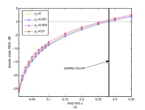
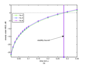
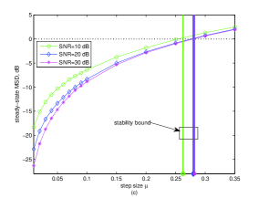
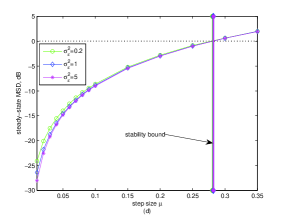
Figure 2: Steady-state MSDs versus step size $\mu$. (a) $N=4$, $\sigma_{\epsilon}^{2}=1$, SNR=30 dB; (b) $p_{r}=0.001$, $\sigma_{\epsilon}^{2}=1$, SNR=30 dB; (c) $N=4$, $\sigma_{\epsilon}^{2}=1$, $p_{r}=0.001$; (d) $N=4$, $p_{r}=0.001$, SNR=30 dB. [$M=32$].

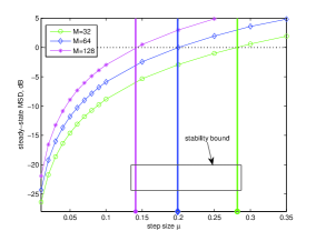
Figure 3: Steady-state MSDs versus step size $\mu$. [$p_{r}=0.001$, $N=4$, $\sigma_{\epsilon}^{2}=1$, SNR=30 dB].

Figs. 4 to 6 check the proposed transient model (19) (where $\rho=0$) for the IWF-SSAF algorithm and compares with the transient model in [15]. As can be seen, the proposed model matches better the simulation than the existing model. This is due mainly to the fact that the existing model relies on the long adaptive filter assumption and the whitening assumption on the decimated subband input vectors, while the proposed model does not require them. For instance, in Fig. 4, the steady-state results for the existing model are closer to the simulations as $M$ increases. It is seen from Fig. 5 that the fixed step-size $\mu$ can not make the IWF-SSAF algorithm reach fast convergence and low steady-state MSD simultaneously. By increasing the number of subbands $N$, the IWF-SSAF algorithm can speed up the convergence, see Fig. 6. Moreover, Figs. 5 and 6 reveal that the theory expression (24) with (26) on the steady-state MSD of the IWF-SSAF algorithm is valid only when the step-size is small.

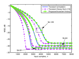
Figure 4: MSD curves of the IWF-SSAF algorithm for different $M$. [$p_{r}=0.001$, $\mu=0.004$, $N=4$, SNR=30 dB].

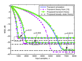
Figure 5: MSD curves of the IWF-SSAF algorithm using different step sizes. [$p_{r}=0.001$, $N=4$, $M=32$, SNR=30 dB].

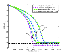
Figure 6: MSD curves of the IWF-SSAF algorithm for different $N$. [$p_{r}=0.001$, $\mu=0.002$, $M=32$, SNR=30 dB].

In Figs. 7 and 8, we check the theoretical insights given in Section IV. B on the S-IWF-SSAF algorithm in sparse scenarios. The sparse vector $\bm{w}^{o}$ of interest has $M=64$ entries, where its NZ entries are Gaussian variables with zero mean and variance of $1/\sqrt{|\text{NZ}|}$ and their positions are randomly selected from the binomial distribution. As one can see in Fig. 7, in terms of the transient MSD of the S-IWF-SSAF algorithm, the theoretical curves obtained from (19) have good fit with the simulated curves. In order to show the better performance of the S-IWF-SSAF algorithm when the parameter vector of interest is sparse (where $|\text{NZ}|=4$) as compared to the IWF-SSAF algorithm, we choose $\rho=4\times 10^{-5}$ in Fig. 7(a) and $\rho=7\times 10^{-5}$ in Fig. 7(b), respectively. Figs. 8 investigates the effect of $\rho$ on the S-IWF-SSAF performance in the steady-state. As declared in theorem 2 or (66), in sparse systems there is a range of values for choosing $\rho$ so that the S-IWF-SSAF algorithm outperforms the IWF-SSAF algorithm. Moreover, this range will gradually die out as $\bm{w}^{o}$ becomes non-sparse (i.e., NZ entries become more).

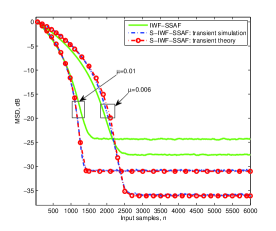
Figure 7: MSD curves of the IWF-SSAF and S-IWF-SSAF algorithms for identifying sparse $\bm{w}^{o}$. [$\xi=0.05$, $p_{r}=0.001$, $N=4$, SNR=30 dB].

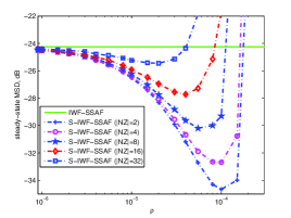
Figure 8: Steady-state MSDs versus $\rho$. [$\xi=0.05$, $p_{r}=0.001$, $\mu=0.01$, $N=4$, SNR=30 dB].

VI-B Comparison of algorithms

In this subsection, we compare the performance of the proposed S-IWF-SSAF and VP-S-IWF-SSAF algorithms with that of the NSAF, BDVSS-SSAF [17], IWF-SSAF, and BDVSS-IWF-SSAF [19] algorithms under the AEC environment. In the hands-free telephone system, the echo is frequently encountered, that is, the talker hears his own time-delayed voice [108]. Concretely, $\bm{w}^{o}$ denotes the acoustic echo channel between loudspeaker and microphone at the near-end. The far-end speech $u(n)$ is played at the loudspeaker, and after passing through $\bm{w}^{o}$ to yield the echo signal $y(n)=\bm{u}^{T}(n)\bm{w}^{o}$; at the same time, the echo signal $y(n)$ is picked up by the microphone and sent to the far-end talker, which impair the quality of the speech. In adaptive AEC, by feeding the same input signal $u(n)$, the output of the adaptive filter $\bm{w}(n)$ will be the replica of the echo, i.e., $\hat{y}(n)=\bm{u}^{T}(n)\bm{w}(n)$, thus by performing $e(n)=d(n)-\hat{y}(n)$ (where the microphone signal $d(n)$ consists of the echo, the background noise $v_{g}(n)$, and the possible near-end speech or impulsive noise $v_{\text{im}}(n)$), we can cancel the echo as $\bm{w}(n)\rightarrow\bm{w}^{o}$. That is to say, the adaptive AEC is a typical adaptive system identification problem that identifies the acoustic echo channel, even if we eventually need the signal $e(n)$. To address the delay issue from the original SAF structure depicted in Fig. 1 for an AEC application, however, Fig. 9 shows its delayless structure [109]. In comparison, the only difference in the delayless structure is that $e(n)$ is calculated in the original sequences through an auxiliary loop by copying $\bm{w}(k)$ to $\bm{w}(n)$ once for every $N$ input samples (i.e., when $n=kN$). Here, the sparse acoustic echo channel is shown in Fig. 10 with $M=512$ taps. We set the number of subbands to $N=8$ for all the SAF algorithms.

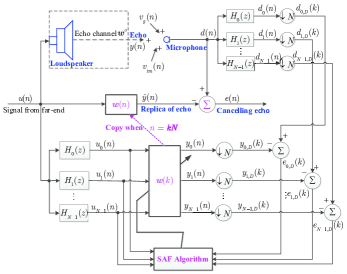
Figure 9: Delayless multiband structure of SAF applied into AEC.

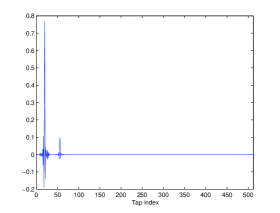
Figure 10: Sparse acoustic echo channel.

In the first example, we consider the (symmetric) $\alpha$-stable process to describe the additive noise $v(n)$ with impulsive samples [3, 5, 34], which is more realistic than the CG process usually used in the analysis. The $\alpha$-stable noise is expressed by $\phi(t)=\exp(-\gamma|t|^{\alpha})$, where the characteristic exponent $0<\alpha\leq 2$ determines the noise’s impulsiveness (whose role behaves like the impulsive noise probability), and $\gamma>0$ indicates the dispersion level of the noise. Note that, when $\alpha=2$, it is the Gaussian noise. In view of acoustic scenarios, we set $\alpha=1.5$ and $\gamma=1/30$ [5]. The normalized MSD, i.e., $\text{NMSD}(n)=10\log 10(\text{MSD}(n)/||\bm{w}^{o}||_{2}^{2})$ is used for measuring the algorithms’ performance. Fig. 11 depicts the NMSD performance of the algorithms for the AR input. In this figure, to compare the tracking capability of these algorithms, $\bm{w}^{o}$ undergoes a sudden change by shifting its 12 taps to the right at the 80001-th input sample. As expected, all the SSAF-type algorithms show stable convergence in the $\alpha$-stable noise, while the NSAF algorithm has severe shaking. Since the IWF-SSAF algorithm employs the band-dependent weighting factors rather than the common one in the SSAF algorithm, the BVDSS-IWF-SSAF algorithm has better convergence than the BDVSS-SSAF algorithm. Due to the sparsity-aware step (7b), the proposed S-IWF-SSAF algorithm significantly enhance the IWF-SSAF’s steady-state performance when identifying sparse channels. Moreover, by proposing the adaptation of $\rho$, the S-IWF-SSAF with $\rho_{o}(k)$ algorithm overcomes the selection problem of $\rho$ in the S-IWF-SSAF algorithm. Benefited from the adaptively adjusting parameters ($\mu$ and $\rho$), the proposed VP-S-IWF-SSAF algorithm is superior to the other algorithms in terms of convergence and steady-state behaviors. It is noticed that like the BDVSS-SSAF and BDVSS-IWF-SSAF algorithms, the VP-S-IWF-SSAF algorithm also cannot track the sudden change of $\bm{w}^{o}$, but this issue can be addressed by applying the reset algorithm (RA) presented in [17]. By using the speech signal as the input, similar results can be obtained in Fig. 12 except the tracking performance.

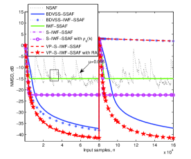
Figure 11: NMSD curves of various SAF algorithms for the AR input. We set the fixed step-size $\mu=0.2$ for the NSAF algorithm and $\mu=0.01$ for the IWF-SSAF, S-IWF-SSAF, and S-IWF-SSAF with $\rho_{o}(k)$ algorithms. The parameter $\rho$ for the S-IWF-SSAF algorithm is chosen as $5\times 10^{-6}$ in a trial and error way. For the proposed sparsity-aware algorithms, we choose $\xi=0.01$, $\chi=2$ for the S-IWF-SSAF with $\rho_{o}(k)$ and $\chi=1$ for the VP-S-IWF-SSAF. Other parameters of algorithms are set as follows: $V_{T}=M$, $\kappa=1$ for the BDVSS-SSAF; $\mu_{U}=0.06$, $\mu_{L}=10^{-5}$, $\kappa=1$ for the BDVSS-IWF-SSAF; $\tau=1$, $\mu_{\min}=10^{-5}$ for the VP-S-IWF-SSAF.

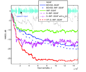
Figure 12: NMSD curves of various SAF algorithms for the speech input (single run). Since the speech signal exists the silent period (zero values), to avoid the division by zero in the algorithms’ update, we add a regularization parameter $\delta$, i.e., $\delta=20\sigma_{u}^{2}/N$ (NSAF and proposed algorithms), $\delta=20\sigma_{u}^{2}$ (BDVSS-SSAF and BDVSS-IWF-SSAF). Some algorithms’ parameters are retuned as $\kappa=2$ (BDVSS-SSAF), $\kappa=3$ (BDVSS-IWF-SSAF), and $\tau=2$ (VP-S-IWF-SSAF).

In the second example, we consider the double-talk case that the near-end speech also appears. In this case, we choose $\alpha=1.8$ for the $\alpha$-stable noise. The NMSD results of the algorithms are shown in Fig. 12. As opposed to the NSAF algorithm, the SSAF-type algorithms (especially for the VSS versions) are insensitive to the double-talk. The VP-S-IWF-SSAF algorithm is still the best choice among these algorithms, because it optimizes the selections of the step-size and the sparsity penalty parameter.

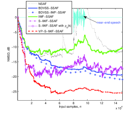
Figure 13: NMSD curves of various SAF algorithms in the double-talk scenario (single run). Parameters setting is the same as in Fig. 12.

VII Conclusion

In this work, the S-IWF-SSAF algorithm was proposed to take advantage of the underlying sparsity of the systems. The theoretical analysis of the S-IWF-SSAF algorithm has been performed that it has significant improvement in the steady-state performance as compared to the IWF-SSAF counterpart when works in sparse system environments. Even for the IWF-SSAF algorithm, the proposed analysis does not require special assumptions, so it matches more accurate with the simulated results than the existing analysis. Moreover, we have developed joint time-varying schemes of both the step-size and the sparsity penalty parameter for the S-IWF-SSAF algorithm, i.e., VP-S-IWF-SSAF, to further improve the convergence and steady-state performance. Simulations in both system identification and AEC situations have been conducted to verify our theoretical analysis and the effectiveness of the proposed algorithms.

It is worth pointing out that, for the proposed VP-S-IWF-SSAF algorithm we simply choose the log-penalty given in (8) from several sparsity-aware strategies as a paradigm. Therefore, in the future, it is also necessary to study the effect of different sparsity-aware strategies with respect to the effectiveness of joint variable parameters in this algorithm.

Appendix  A Derivation of (13a)

Taking the expectation for both sides of (10a), we have

$$\text{E}\{\widetilde{\bm{\varphi}}(k+1)\}=\text{E}\{\widetilde{\bm{w}}(k)\}-\mu\sum\limits_{i=0}^{N-1}\text{E}\left\{\frac{\text{sgn}(e_{i,D}(k))\bm{u}_{i}(k)}{\|\bm{u}_{i}(k)\|_{2}}\right\}.$$ (50)

To compute the last expectation in (50), we introduce the conditional expectation:

$$\text{E}\left\{\frac{\text{sgn}(e_{i,D}(k))\bm{u}_{i}(k)}{\|\bm{u}_{i}(k)\|_{2}}\right\}=$$ (51)

$$\;\;\;\;\;\;\;\;\;\;\;\;\;\;\;\;\;\;\text{E}\left\{\text{E}\left\{\frac{\text{sgn}(e_{i,D}(k))\bm{u}_{i}(k)}{\|\bm{u}_{i}(k)\|_{2}}\left|\widetilde{\bm{w}}(k)\right.\right\}\right\}.$$

Since $\bm{h}_{i}$ is deterministic, it follows (11) and assumption 2 that $v_{i,D}(k)$ can also be referred to as a CG process, i.e., $v_{i,D}(k)=v_{\text{g},i,D}(k)+b_{i}(k)\eta_{i,D}(k)$, where $v_{\text{g},i,D}(k)$ and $\eta_{i,D}(k)$ are zero-mean white Gaussian with variances $\sigma_{\text{g},i}^{2}=||\bm{h}_{i}||_{2}^{2}\sigma_{\text{g}}^{2}$ and $\sigma_{\eta,i}^{2}=||\bm{h}_{i}||_{2}^{2}\sigma_{\eta}^{2}$ respectively, and $b_{i}(k)$ obeys the Bernoulli distribution with $P\{b_{i}(k)=1\}=p_{r}$ being the probability of occurring 1. It should be stressed that if the analysis filter bank for partitioning the input signal $u(n)$ and the desired signal $d(n)$ is assumed to be identical and paraunitary, as done in references [26] for analyzing the NSAF algorithm, then $||\bm{h}_{i}||_{2}^{2}=1/N$ will be further given.

Hence, applying the CG noise model and the law of total probability, the following relation is established:

$$\text{E}\left\{\frac{\text{sgn}(e_{i,D}(k))\bm{u}_{i}(k)}{\|\bm{u}_{i}(k)\|_{2}}\left|\widetilde{\bm{w}}(k)\right.\right\}=$$ (52)

$$P\{b(k)=1\}\text{E}\left\{\frac{\text{sgn}(e_{i,D,1}(k))\bm{u}_{i}(k)}{\|\bm{u}_{i}(k)\|_{2}}\left|\widetilde{\bm{w}}(k)\right.\right\}+$$

$$P\{b(k)=0\}\text{E}\left\{\frac{\text{sgn}(e_{i,D,2}(k))\bm{u}_{i}(k)}{\|\bm{u}_{i}(k)\|_{2}}\left|\widetilde{\bm{w}}(k)\right.\right\}=$$

$$\;\;\;\;\;\;\;\;\;\;\;\;\;\;p_{r}\text{E}\left\{\frac{\text{sgn}(e_{i,D,1}(k))\bm{u}_{i}(k)}{\|\bm{u}_{i}(k)\|_{2}}\left|\widetilde{\bm{w}}(k)\right.\right\}+$$

$$\;\;\;\;\;\;\;\;\;\;\;\;\;\;(1-p_{r})\text{E}\left\{\frac{\text{sgn}(e_{i,D,2}(k))\bm{u}_{i}(k)}{\|\bm{u}_{i}(k)\|_{2}}\left|\widetilde{\bm{w}}(k)\right.\right\},$$

where $e_{i,D,1}(k)=e_{i,a}(k)+v_{\text{g},i,D}(k)+\eta_{i,D}(k)$ and $e_{i,D,2}(k)=e_{i,a}(k)+v_{\text{g},i,D}(k)$.

Both $v_{\text{g},i,D}(k)$ and $\eta_{i,D}(k)$ are Gaussian random variables, thus we can assume $e_{i,D,1}(k)$ and $e_{i,D,2}(k)$ to be zero mean Gaussian variables when $M$ is large [110]. Accordingly, based on Price’s theorem and assumption 3, we have

$$\text{E}\left\{\frac{\text{sgn}(e_{i,D,1}(k))\bm{u}_{i}(k)}{\|\bm{u}_{i}(k)\|_{2}}\left|\widetilde{\bm{w}}(k)\right.\right\}=$$ (53)

$$\;\;\;\;\;\;\;\;\;\;\;\sqrt{\frac{2}{\pi}}\frac{1}{\sqrt{\text{E}\{e_{i,D,1}^{2}(k)\}}}\text{E}\{\bm{A}_{i}(k)\}\widetilde{\bm{w}}(k),$$

and

$$\text{E}\left\{\frac{\text{sgn}(e_{i,D,2}(k))\bm{u}_{i}(k)}{\|\bm{u}_{i}(k)\|_{2}}\left|\widetilde{\bm{w}}(k)\right.\right\}=$$ (54)

$$\;\;\;\;\;\;\;\;\;\;\;\sqrt{\frac{2}{\pi}}\frac{1}{\sqrt{\text{E}\{e_{i,D,2}^{2}(k)\}}}\text{E}\{\bm{A}_{i}(k)\}\widetilde{\bm{w}}(k),$$

where $\bm{A}_{i}(k)=\frac{\bm{u}_{i}(k)\bm{u}_{i}^{\text{T}}(k)}{\|\bm{u}_{i}(k)\|_{2}}$.

By substituting (51)-(54) into (50), we will obtain  (13a).

Appendix  B Derivation of (19a)

Both sides of (10a) are multiplied by their transposes, then we take the expectations of all the terms to yield

$$\widetilde{\bm{\varPhi}} (k+1)=\widetilde{\bm{W}}(k)-$$ (55)

$$\mu\sum\limits_{i=0}^{N-1}\underbrace{\text{E}\left\{\frac{\widetilde{\bm{w}}(k)\text{sgn}(e_{i,D}(k))\bm{u}_{i}^{\text{T}}(k)}{\|\bm{u}_{i}(k)\|_{2}}\right\}}\limits_{\text{I}}-$$

$$\mu\sum\limits_{i=0}^{N-1}\underbrace{\text{E}\left\{\frac{\bm{u}_{i}(k)\text{sgn}(e_{i,D}(k))\widetilde{\bm{w}}^{\text{T}}(k)}{\|\bm{u}_{i}(k)\|_{2}}\right\}}\limits_{\text{II}}+$$

$$\mu^{2}\underbrace{\text{E}\left\{\sum\limits_{i=0}^{N-1}\frac{\bm{u}_{i}(k)\text{sgn}(e_{i,D}(k))}{\|\bm{u}_{i}(k)\|_{2}}\sum\limits_{j=0}^{N-1}\frac{\bm{u}_{j}^{\text{T}}(k)\text{sgn}(e_{j,D}(k))}{\|\bm{u}_{j}(k)\|_{2}}\right\}}\limits_{\text{III}},$$

By performing similar procedures to those in (51)-(54), the term I in (55) can be calculated by

$$\text{E}\left\{\frac{\widetilde{\bm{w}}(k)\text{sgn}(e_{i,D}(k))\bm{u}_{i}^{\text{T}}(k)}{\|\bm{u}_{i}(k)\|_{2}}\right\}=\widetilde{\bm{W}}(k)\Omega_{i}(k)\text{E}\{\bm{A}_{i}(k)\},$$ (56)

but we omit this derivation for brevity. The term II in (55) is the transpose of (56), i.e.,

$$\text{E}\left\{\frac{\bm{u}_{i}(k)\text{sgn}(e_{i,D}(k))\widetilde{\bm{w}}^{\text{T}}(k)}{\|\bm{u}_{i}(k)\|_{2}}\right\}=\Omega_{i}(k)\text{E}\{\bm{A}_{i}(k)\}\widetilde{\bm{W}}(k).$$ (57)

The term III in (55) can be approximated as $\sum\limits_{i=0}^{N-1}\text{E}\{\check{\bm{A}}_{i}(k)\}$, where $\check{\bm{A}}_{i}(k)=\frac{\bm{u}_{i}(k)\bm{u}_{i}^{\text{T}}(k)}{\|\bm{u}_{i}(k)\|_{2}^{2}}$, because different subband vectors $\bm{u}_{i}(k)$ and $\bm{u}_{j}(k)$ are weakly correlated [2, 26]. With these relations, it is easy to derive (19a) from (55).

Appendix  C

For ease of evaluating $\text{E}\{H^{\prime}(\bm{\varphi}(k))\}$, $\bm{\varTheta}(k)$, and $\bm{\varXi}(k)$, we need another two assumptions. They have been frequently called up for simplifying the analyses of sparsity-aware adaptive filtering algorithms [36, 39, 112].

Assumption 4: The $m$-th component of the intermediate weights error vector $\widetilde{\bm{\varphi}}(k)$ for every $k$, has a Gaussian distribution, namely, $\widetilde{\varphi}_{m}(k)\sim\aleph(z_{m}(k),\sigma_{m}^{2}(k))$, where the mean $z_{m}(k)$ is the $m$-th component of $\text{E}\{\widetilde{\bm{\varphi}}(k)\}$ from (13a) and the variance $\sigma_{m}^{2}(k)$ is computed from (19a) by $\sigma_{m}^{2}(k)=\widetilde{\bm{\varPhi}}_{m,m}(k)-z_{m}^{2}(k)$. As such, $\varphi_{m}(k)$ follows the distribution $\aleph(\bar{\varphi}_{m},\sigma_{\varphi,m}^{2})$ with $\bar{\varphi}_{m}=w_{m}^{o}-z_{m}(k)$ and $\sigma_{\varphi,m}^{2}=\sigma_{m}^{2}(k)$ where $w_{m}^{o}$ is the $m$-th component of $\bm{w}^{o}$.

Assumption 5: When $m\neq l$, it can be assumed that $\text{E}\{H^{\prime}(\varphi_{m}(k))\varphi_{l}(k)\}\approx\text{E}\{H^{\prime}(\varphi_{m}(k))\}\text{E}\{\varphi_{l}(k)\}$ and $\text{E}\{H^{\prime}(\varphi_{m}(k))H^{\prime}(\varphi_{l}(k))\}\approx\text{E}\{H^{\prime}(\varphi_{m}(k))\}\text{E}\{H^{\prime}(\varphi_{l}(k))\}$.

Based on assumption 4, we compute the $m$-th component of $\text{E}\{H^{\prime}(\bm{\varphi}(k)\}$ by

$$\text{E}\{H^{\prime}(\varphi_{m}(k))\}\approx\frac{\text{E}\{\text{sgn}(\varphi_{m}(k))\}}{\xi+\text{E}\{|\varphi_{m}(k)|\}},$$ (58)

where this approximation also because $\xi$ is relatively small, and

$$\begin{array}[]{rcl}\begin{aligned} \text{E}\{|\varphi|\}=&\frac{1}{\sqrt{2\pi}\sigma_{\varphi}}\int_{-\infty}^{\infty}|\varphi|\exp^{-\left(\frac{\varphi-\bar{\varphi}}{\sqrt{2}\sigma_{\varphi}}\right)^{2}}d\varphi\\ =&\sqrt{\frac{2}{\pi}}\sigma_{\varphi}\exp^{-\frac{\bar{\varphi}^{2}}{2\sigma_{\varphi}^{2}}}+\bar{\varphi}\text{erf}\left(\frac{\bar{\varphi}}{\sqrt{2}\sigma_{\varphi}}\right),\end{aligned}\end{array}$$ (59)

and

$$\begin{array}[]{rcl}\begin{aligned} \text{E}\{\text{sgn}(\varphi)\}=&\frac{1}{\sqrt{2\pi}\sigma_{\varphi}}\int_{-\infty}^{\infty}\text{sgn}(\varphi)\exp^{-\left(\frac{\varphi-\bar{\varphi}}{\sqrt{2}\sigma_{\varphi}}\right)^{2}}d\varphi\\ =&\text{erf}\left(\frac{\bar{\varphi}}{\sqrt{2}\sigma_{\varphi}}\right)\end{aligned}\end{array}$$ (60)

with $\text{erf}(\varphi)\triangleq\frac{2}{\sqrt{\pi}}\int_{0}^{\varphi}\exp^{-t^{2}}dt$. It has been given that $\bm{\varTheta}_{m,l}(k)\triangleq\text{E}\{H^{\prime}(\varphi_{m}(k))\}{w_{l}^{o}}-\text{E}\{H^{\prime}(\varphi_{m}(k))\varphi_{l}(k)\}$ and $\bm{\varXi}_{m,l}(k)\triangleq\text{E}\{H^{\prime}(\varphi_{m}(k))H^{\prime}(\varphi_{l}(k))\}$ for any $m,l$. Specifically, when $m=l$, we have

$$\text{E}\{H^{\prime}(\varphi_{m}(k))\varphi_{m}(k)\}\approx\frac{\text{E}\{|\varphi_{m}(k)|\}}{\xi+\text{E}\{|\varphi_{m}(k)|\}}$$ (61)

and

$$\text{E}\{H^{\prime}(\varphi_{m}(k))^{2}\}\approx\frac{1}{\xi^{2}+2\xi\text{E}\{|\varphi_{m}(k)|\}+\text{E}\{\varphi_{m}^{2}(k)\}}.$$ (62)

When $m\neq l$, according to assumption 5 we can obtain

$$\text{E}\{H^{\prime}(\varphi_{m}(k))\varphi_{l}(k)\}\approx\frac{\text{E}\{\text{sgn}(\varphi_{m}(k))\}}{\xi+\text{E}\{|\varphi_{m}(k)|\}}\text{E}\{\varphi_{l}(k)\}$$ (63)

and

$$\text{E}\{H^{\prime}(\varphi_{m}(k))H^{\prime}(\varphi_{l}(k))\}\approx\frac{\text{E}\{\text{sgn}(\varphi_{m}(k))\}}{\xi+\text{E}\{|\varphi_{m}(k)|\}}\frac{\text{E}\{\text{sgn}(\varphi_{l}(k))\}}{\xi+\text{E}\{|\varphi_{l}(k)|\}}.$$ (64)

Appendix  D Possibility of $\Delta_{s}(\infty)<0$

The matrix $(\bm{I}_{M^{2}}-\bm{F}_{\infty})$ is positive definite due to the convergence of the algorithm. As such, it can be approximated by $(\bm{I}_{M^{2}}-\bm{F}_{\infty})\approx t\cdot\bm{I}_{M^{2}}$ [113], where $t>0$ is finite. In this case, we are able to simplify $\Delta_{s}(\infty)$ given in (25) as

$$\begin{array}[]{rcl}\begin{aligned} \Delta_{s}&(\infty)\approx\frac{1}{t}\text{vec}^{\text{T}}(\bm{I}_{M})\text{vec}\left(\rho\bm{\varTheta}(\infty)+\rho\bm{\varTheta}^{\text{T}}(\infty)+\rho^{2}\bm{\varXi}(\infty)\right)\\ =&\frac{1}{t}\left[2\rho\text{E}\{\widetilde{\bm{\varphi}}^{\text{T}}(\infty)H^{\prime}(\bm{\varphi}(\infty))\}+\rho^{2}\text{E}\{||H^{\prime}(\bm{\varphi}(\infty))||_{2}^{2}\}\right],\\ =&\frac{\rho}{t}\text{E}\{||H^{\prime}(\bm{\varphi}(\infty))||_{2}^{2}\}\left[\rho+\frac{2\text{E}\{\widetilde{\bm{\varphi}}^{\text{T}}(\infty)H^{\prime}(\bm{\varphi}(\infty))\}}{\text{E}\{||H^{\prime}(\bm{\varphi}(\infty))||_{2}^{2}\}}\right].\end{aligned}\end{array}$$ (65)

Obviously, $\Delta_{s}(\infty)<0$ is true if and only if

$$\begin{array}[]{rcl}\begin{aligned} 0<\rho<-\frac{2\text{E}\{\widetilde{\bm{\varphi}}^{\text{T}}(\infty)H^{\prime}(\bm{\varphi}(\infty))\}}{\text{E}\{||H^{\prime}(\bm{\varphi}(\infty))||_{2}^{2}\}}\triangleq\rho_{\text{up}}\end{aligned}\end{array}$$ (66)

and

$$\begin{array}[]{rcl}\begin{aligned} \text{E}\{\widetilde{\bm{\varphi}}^{\text{T}}(\infty)H^{\prime}(\bm{\varphi}(\infty))\}<0.\end{aligned}\end{array}$$ (67)

The above relations shows that $\text{E}\{\widetilde{\bm{\varphi}}^{\text{T}}(\infty)H^{\prime}(\bm{\varphi}(\infty))\}<0$ is a necessary condition to $\Delta_{s}(\infty)<0$ in the scenario that the vector $\bm{w}^{o}$ to be estimated is sparse. In particular, the number of zero elements (Z set) in $\bm{w}^{o}$ are much more than that of non-zero elements (NZ set).

Since $H(\cdot)$ is a real-valued convex function, from the definition of the sub-gradient [39, 114], the following inequality will hold:

$$\begin{array}[]{rcl}\begin{aligned} \widetilde{\bm{\varphi}}^{\text{T}}(\infty)H^{\prime}(\bm{\varphi}(\infty))&=(\bm{w}^{o}-\bm{\varphi}(\infty))^{\text{T}}H^{\prime}(\bm{\varphi}(\infty))\\ &\leq H(\bm{w}^{o})-H(\bm{\varphi}(\infty)).\end{aligned}\end{array}$$ (68)

Since the penalty function $H(\bm{w})$ in (8) measures the sparsity of the vector $\bm{w}$ and undoubtedly, the true vector $\bm{w}^{o}$ is more sparse than its estimate $\bm{\varphi}(\infty)$ obtaining from the gradient update (7a), it is expected that

$$\begin{array}[]{rcl}\begin{aligned} H(\bm{w}^{o})-H(\bm{\varphi}(\infty))&\approx-\sum_{m\in\text{Z set}}^{M}\ln(1+|\varphi_{m}(\infty)|/\xi)\\ &<0.\end{aligned}\end{array}$$ (69)

Consequently, by appropriately choosing the sparse penalty parameter $\rho$, the condition $\Delta_{s}(\infty)<0$ is likely to be true. Conversely, when $\bm{w}^{o}$ is not sparse, (69) would not hold so that $\Delta_{s}(\infty)<0$ is impossible regardless of $\rho$.

References

- [1] A. H. Sayed, Fundamentals of adaptive filtering. John Wiley & Sons, 2003.
- [2] K.-A. Lee, W.-S. Gan, and S. M. Kuo, Subband adaptive filtering: theory and implementation. John Wiley & Sons, 2009.
- [3] C. L. Nikias and M. Shao, Signal processing with alpha-stable distributions and applications. Wiley-Interscience, 1995.
- [4] M. Zimmermann and K. Dostert, “Analysis and modeling of impulsive noise in broad-band powerline communications,” IEEE Transactions on Electromagnetic Compatibility, vol. 44, no. 1, pp. 249–258, 2002.
- [5] P. G. Georgiou, P. Tsakalides, and C. Kyriakakis, “Alpha-stable modeling of noise and robust time-delay estimation in the presence of impulsive noise,” IEEE Transactions on Multimedia, vol. 1, no. 3, pp. 291–301, 1999.
- [6] L. R. Vega, H. Rey, J. Benesty, and S. Tressens, “A new robust variable step-size NLMS algorithm,” IEEE Transactions on Signal Processing, vol. 56, no. 5, pp. 1878–1893, 2008.
- [7] Y. Yu, L. Lu, Z. Zheng, W. Wang, Y. Zakharov, and R. C. de Lamare, “DCD-based recursive adaptive algorithms robust against impulsive noise,” IEEE Transactions on Circuits and Systems II: Express Briefs, vol. 67, no. 7, pp. 1359–1363, 2020.
- [8] L. Dang, B. Chen, S. Wang, Y. Gu, and J. C. Príncipe, “Kernel kalman filtering with conditional embedding and maximum correntropy criterion,” IEEE Transactions on Circuits and Systems I: Regular Papers, vol. 66, no. 11, pp. 4265–4277, 2019.
- [9] V. Mathews and S. Cho, “Improved convergence analysis of stochastic gradient adaptive filters using the sign algorithm,” IEEE Transactions on Acoustics, Speech, and Signal Processing, vol. 35, no. 4, pp. 450–454, 1987.
- [10] B. Chen, L. Xing, H. Zhao, N. Zheng, and J. C. Príncipe, “Generalized correntropy for robust adaptive filtering,” IEEE Transactions on Signal Processing, vol. 64, no. 13, pp. 3376–3387, 2016.
- [11] B. Chen, L. Xing, B. Xu, H. Zhao, N. Zheng, and J. C. Príncipe, “Kernel risk-sensitive loss: definition, properties and application to robust adaptive filtering,” IEEE Transactions on Signal Processing, vol. 65, no. 11, pp. 2888–2901, 2017.
- [12] B. Chen, L. Xing, J. Liang, N. Zheng, and J. C. Principe, “Steady-state mean-square error analysis for adaptive filtering under the maximum correntropy criterion,” IEEE Signal Processing Letters, vol. 21, no. 7, pp. 880–884, 2014.
- [13] K.-A. Lee and W.-S. Gan, “Improving convergence of the NLMS algorithm using constrained subband updates,” IEEE Signal Processing Letters, vol. 11, no. 9, pp. 736–739, 2004.
- [14] J. Ni and F. Li, “Variable regularisation parameter sign subband adaptive filter,” Electronics Letters, vol. 46, no. 24, pp. 1605–1607, 2010.
- [15] Y. Yu and H. Zhao, “Novel sign subband adaptive filter algorithms with individual weighting factors,” Signal Processing, vol. 122, pp. 14–23, 2016.
- [16] J. Shin, J. Yoo, and P. Park, “Variable step-size sign subband adaptive filter,” IEEE Signal Processing Letters, vol. 20, no. 2, pp. 173–176, 2013.
- [17] J. Yoo, J. Shin, and P. Park, “A band-dependent variable step-size sign subband adaptive filter,” Signal Processing, vol. 104, pp. 407–411, 2014.
- [18] J. Kim, J.-H. Chang, and S. W. Nam, “Sign subband adaptive filter with -norm minimisation-based variable step-size,” Electronics Letters, vol. 49, no. 21, pp. 1325–1326, 2013.
- [19] J.-H. Kim, J. Kim, J. H. Jeon, and S. W. Nam, “Delayless individual-weighting-factors sign subband adaptive filter with band-dependent variable step-sizes,” IEEE/ACM Transactions on Audio, Speech, and Language Processing, vol. 25, no. 7, pp. 1526–1534, 2017.
- [20] P. Wen and J. Zhang, “Robust variable step-size sign subband adaptive filter algorithm against impulsive noise,” Signal Processing, vol. 139, pp. 110–115, 2017.
- [21] T. K. Paul and T. Ogunfunmi, “On the convergence behavior of the affine projection algorithm for adaptive filters,” IEEE Transactions on Circuits and Systems I: Regular Papers, vol. 58, no. 8, pp. 1813–1826, 2011.
- [22] Z. Zheng, Z. Liu, and Y. Dong, “Steady-state and tracking analyses of the improved proportionate affine projection algorithm,” IEEE Transactions on Circuits and Systems II: Express Briefs, vol. 65, no. 11, pp. 1793–1797, 2017.
- [23] S. J. de Almeida, J. C. M. Bermudez, N. J. Bershad, and M. H. Costa, “A statistical analysis of the affine projection algorithm for unity step size and autoregressive inputs,” IEEE Transactions on Circuits and Systems I: Regular Papers, vol. 52, no. 7, pp. 1394–1405, 2005.
- [24] Z. Zheng and Z. Liu, “Steady-state mean-square performance analysis of the affine projection sign algorithm,” IEEE Transactions on Circuits and Systems II: Express Briefs, 2019. doi:10.1109/TCSII.2019.2946782.
- [25] Z. Zheng, Z. Liu, H. Zhao, Y. Yu, and L. Lu, “Robust set-membership normalized subband adaptive filtering algorithms and their application to acoustic echo cancellation,” IEEE Transactions on Circuits and Systems I: Regular Papers, vol. 64, no. 8, pp. 2098–2111, 2017.
- [26] W. Yin and A. S. Mehr, “Stochastic analysis of the normalized subband adaptive filter algorithm,” IEEE Transactions on Circuits and Systems I: Regular Papers, vol. 58, no. 5, pp. 1020–1033, 2011.
- [27] J. Shin, J. Yoo, and P. Park, “Adaptive regularisation for normalised subband adaptive filter: mean-square performance analysis approach,” IET Signal Processing, vol. 12, no. 9, pp. 1146–1153, 2018.
- [28] J. J. Jeong, S. H. Kim, G. Koo, and S. W. Kim, “Mean-square deviation analysis of multiband-structured subband adaptive filter algorithm,” IEEE Transactions on Signal Processing, vol. 64, no. 4, pp. 985–994, 2016.
- [29] S. Zhang and W. X. Zheng, “Mean-square analysis of multi-sampled multiband-structured subband filtering algorithm,” IEEE Transactions on Circuits and Systems I: Regular Papers, vol. 66, no. 3, pp. 1051–1062, 2019.
- [30] Y. Yu, H. Zhao, and B. Chen, “Steady-state mean-square-deviation analysis of the sign subband adaptive filter algorithm,” Signal Processing, vol. 120, pp. 36–42, 2016.
- [31] J. Shin, J. Yoo, and P. Park, “Steady-state mean-square deviation analysis of the sign subband adaptive filter,” Electronics Letters, vol. 53, no. 12, pp. 793–795, 2017.
- [32] J. Radecki, Z. Zilic, and K. Radecka, “Echo cancellation in IP networks,” in The 2002 45th Midwest Symposium on Circuits and Systems, 2002. MWSCAS-2002., vol. 2, 2002, pp. II–II.
- [33] E. Hänsler and G. Schmidt, Topics in acoustic echo and noise control. Springer-Verlag, 2006.
- [34] K. Pelekanakis and M. Chitre, “Adaptive sparse channel estimation under symmetric alpha-stable noise,” IEEE Transactions on wireless communications, vol. 13, no. 6, pp. 3183–3195, 2014.
- [35] W. F. Schreiber, “Advanced television systems for terrestrial broadcasting: Some problems and some proposed solutions,” Proceedings of the IEEE, vol. 83, no. 6, pp. 958–981, 1995.
- [36] D. B. Haddad and M. R. Petraglia, “Transient and steady-state MSE analysis of the IMPNLMS algorithm,” Digital Signal Processing, vol. 33, pp. 50–59, 2014.
- [37] Y. Gu, J. Jin, and S. Mei, “-norm constraint LMS algorithm for sparse system identification,” IEEE Signal Processing Letters, vol. 16, no. 9, pp. 774–777, 2009.
- [38] R. C. de Lamare and R. Sampaio-Neto, “Sparsity-aware adaptive algorithms based on alternating optimization and shrinkage,” IEEE Signal Processing Letters, vol. 21, no. 2, pp. 225–229, 2014.
- [39] Y. Yu, H. Zhao, R. C. de Lamare, and L. Lu, “Sparsity-aware subband adaptive algorithms with adjustable penalties,” Digital Signal Processing, vol. 84, pp. 93–106, 2019.
- [40] Y.-S. Choi, “A new subband adaptive filtering algorithm for sparse system identification with impulsive noise,” Journal of Applied Mathematics, vol. 2014, 2014.
- [41] Z. Shen, T. Huang, and K. Zhou, “-norm constraint normalized logarithmic subband adaptive filter algorithm,” Signal, Image and Video Processing, vol. 12, no. 5, pp. 861–868, 2018.
- [42] Y. Yu, H. He, T. Yang, X. Wang, and R. C. de Lamare, “Diffusion normalized least mean M-estimate algorithms: design and performance analysis,” IEEE Transactions on Signal Processing, vol. 68, pp. 2199–2214, 2020.
- [43] R. C. De Lamare and R. Sampaio-Neto, “Minimum mean-squared error iterative successive parallel arbitrated decision feedback detectors for ds-cdma systems,” IEEE Transactions on Communications, vol. 56, no. 5, pp. 778–789, May 2008.
- [44] P. Li, R. C. de Lamare, and R. Fa, “Multiple feedback successive interference cancellation detection for multiuser mimo systems,” IEEE Transactions on Wireless Communications, vol. 10, no. 8, pp. 2434–2439, August 2011.
- [45] K. Zu, R. C. de Lamare, and M. Haardt, “Generalized design of low-complexity block diagonalization type precoding algorithms for multiuser mimo systems,” IEEE Transactions on Communications, vol. 61, no. 10, pp. 4232–4242, October 2013.
- [46] P. Clarke and R. C. de Lamare, “Transmit diversity and relay selection algorithms for multirelay cooperative mimo systems,” IEEE Transactions on Vehicular Technology, vol. 61, no. 3, pp. 1084–1098, March 2012.
- [47] R. C. de Lamare, “Adaptive and iterative multi-branch mmse decision feedback detection algorithms for multi-antenna systems,” IEEE Transactions on Wireless Communications, vol. 12, no. 10, pp. 5294–5308, October 2013.
- [48] ——, “Massive mimo systems: Signal processing challenges and future trends,” URSI Radio Science Bulletin, vol. 2013, no. 347, pp. 8–20, Dec 2013.
- [49] W. Zhang, H. Ren, C. Pan, M. Chen, R. C. de Lamare, B. Du, and J. Dai, “Large-scale antenna systems with ul/dl hardware mismatch: Achievable rates analysis and calibration,” IEEE Transactions on Communications, vol. 63, no. 4, pp. 1216–1229, April 2015.
- [50] T. Peng, R. C. de Lamare, and A. Schmeink, “Adaptive distributed space-time coding based on adjustable code matrices for cooperative mimo relaying systems,” IEEE Transactions on Communications, vol. 61, no. 7, pp. 2692–2703, July 2013.
- [51] Y. Cai, R. C. d. Lamare, and R. Fa, “Switched interleaving techniques with limited feedback for interference mitigation in ds-cdma systems,” IEEE Transactions on Communications, vol. 59, no. 7, pp. 1946–1956, July 2011.
- [52] P. Li and R. C. de Lamare, “Distributed iterative detection with reduced message passing for networked mimo cellular systems,” IEEE Transactions on Vehicular Technology, vol. 63, no. 6, pp. 2947–2954, July 2014.
- [53] K. Zu and R. C. d. Lamare, “Low-complexity lattice reduction-aided regularized block diagonalization for mu-mimo systems,” IEEE Communications Letters, vol. 16, no. 6, pp. 925–928, June 2012.
- [54] K. Zu, R. C. de Lamare, and M. Haardt, “Generalized design of low-complexity block diagonalization type precoding algorithms for multiuser mimo systems,” IEEE Transactions on Communications, vol. 61, no. 10, pp. 4232–4242, October 2013.
- [55] W. Zhang, R. C. de Lamare, C. Pan, M. Chen, J. Dai, B. Wu, and X. Bao, “Widely linear precoding for large-scale mimo with iqi: Algorithms and performance analysis,” IEEE Transactions on Wireless Communications, vol. 16, no. 5, pp. 3298–3312, May 2017.
- [56] L. T. N. Landau and R. C. de Lamare, “Branch-and-bound precoding for multiuser mimo systems with 1-bit quantization,” IEEE Wireless Communications Letters, vol. 6, no. 6, pp. 770–773, Dec 2017.
- [57] K. Zu, R. C. de Lamare, and M. Haardt, “Multi-branch tomlinson-harashima precoding design for mu-mimo systems: Theory and algorithms,” IEEE Transactions on Communications, vol. 62, no. 3, pp. 939–951, March 2014.
- [58] L. Zhang, Y. Cai, R. C. de Lamare, and M. Zhao, “Robust multibranch tomlinson-harashima precoding design in amplify-and-forward mimo relay systems,” IEEE Transactions on Communications, vol. 62, no. 10, pp. 3476–3490, Oct 2014.
- [59] T. Peng and R. C. de Lamare, “Adaptive buffer-aided distributed space-time coding for cooperative wireless networks,” IEEE Transactions on Communications, vol. 64, no. 5, pp. 1888–1900, May 2016.
- [60] A. G. D. Uchoa, C. T. Healy, and R. C. de Lamare, “Iterative detection and decoding algorithms for mimo systems in block-fading channels using ldpc codes,” IEEE Transactions on Vehicular Technology, vol. 65, no. 4, pp. 2735–2741, April 2016.
- [61] Z. Shao, R. C. de Lamare, and L. T. N. Landau, “Iterative detection and decoding for large-scale multiple-antenna systems with 1-bit adcs,” IEEE Wireless Communications Letters, vol. 7, no. 3, pp. 476–479, June 2018.
- [62] Z. Shao, L. T. N. Landau, and R. C. De Lamare, “Channel estimation for large-scale multiple-antenna systems using 1-bit adcs and oversampling,” IEEE Access, vol. 8, pp. 85 243–85 256, 2020.
- [63] R. B. Di Renna and R. C. de Lamare, “Adaptive activity-aware iterative detection for massive machine-type communications,” IEEE Wireless Communications Letters, pp. 1–1, 2019.
- [64] J. Gu, R. C. de Lamare, and M. Huemer, “Buffer-aided physical-layer network coding with optimal linear code designs for cooperative networks,” IEEE Transactions on Communications, vol. 66, no. 6, pp. 2560–2575, June 2018.
- [65] Y. Jiang, Y. Zou, H. Guo, T. A. Tsiftsis, M. R. Bhatnagar, R. C. de Lamare, and Y. Yao, “Joint power and bandwidth allocation for energy-efficient heterogeneous cellular networks,” IEEE Transactions on Communications, vol. 67, no. 9, pp. 6168–6178, Sep. 2019.
- [66] F. L. Duarte and R. C. de Lamare, “Cloud-driven multi-way multiple-antenna relay systems: Joint detection, best-user-link selection and analysis,” IEEE Transactions on Communications, vol. 68, no. 6, pp. 3342–3354, 2020.
- [67] R. B. D. Renna and R. C. D. Lamare, “Iterative list detection and decoding for massive machine-type communications,” IEEE Transactions on Communications, pp. 1–1, 2020.
- [68] R. C. de Lamare and R. Sampaio-Neto, “Adaptive reduced-rank mmse filtering with interpolated fir filters and adaptive interpolators,” IEEE Signal Processing Letters, vol. 12, no. 3, pp. 177–180, March 2005.
- [69] ——, “Adaptive interference suppression for ds-cdma systems based on interpolated fir filters with adaptive interpolators in multipath channels,” IEEE Transactions on Vehicular Technology, vol. 56, no. 5, pp. 2457–2474, Sep. 2007.
- [70] ——, “Reduced-rank adaptive filtering based on joint iterative optimization of adaptive filters,” IEEE Signal Processing Letters, vol. 14, no. 12, pp. 980–983, Dec 2007.
- [71] R. C. de Lamare, M. Haardt, and R. Sampaio-Neto, “Blind adaptive constrained reduced-rank parameter estimation based on constant modulus design for cdma interference suppression,” IEEE Transactions on Signal Processing, vol. 56, no. 6, pp. 2470–2482, June 2008.
- [72] N. Song, R. C. de Lamare, M. Haardt, and M. Wolf, “Adaptive widely linear reduced-rank interference suppression based on the multistage wiener filter,” IEEE Transactions on Signal Processing, vol. 60, no. 8, pp. 4003–4016, Aug 2012.
- [73] R. C. de Lamare and R. Sampaio-Neto, “Adaptive reduced-rank processing based on joint and iterative interpolation, decimation, and filtering,” IEEE Transactions on Signal Processing, vol. 57, no. 7, pp. 2503–2514, July 2009.
- [74] M. Yukawa, R. C. de Lamare, and R. Sampaio-Neto, “Efficient acoustic echo cancellation with reduced-rank adaptive filtering based on selective decimation and adaptive interpolation,” IEEE Transactions on Audio, Speech, and Language Processing, vol. 16, no. 4, pp. 696–710, May 2008.
- [75] R. C. de Lamare, R. Sampaio-Neto, and M. Haardt, “Blind adaptive constrained constant-modulus reduced-rank interference suppression algorithms based on interpolation and switched decimation,” IEEE Transactions on Signal Processing, vol. 59, no. 2, pp. 681–695, Feb 2011.
- [76] R. C. de Lamare and R. Sampaio-Neto, “Reduced-rank space-time adaptive interference suppression with joint iterative least squares algorithms for spread-spectrum systems,” IEEE Transactions on Vehicular Technology, vol. 59, no. 3, pp. 1217–1228, March 2010.
- [77] ——, “Adaptive reduced-rank equalization algorithms based on alternating optimization design techniques for mimo systems,” IEEE Transactions on Vehicular Technology, vol. 60, no. 6, pp. 2482–2494, July 2011.
- [78] R. Fa and R. C. De Lamare, “Reduced-rank stap algorithms using joint iterative optimization of filters,” IEEE Transactions on Aerospace and Electronic Systems, vol. 47, no. 3, pp. 1668–1684, July 2011.
- [79] R. Fa, R. C. de Lamare, and L. Wang, “Reduced-rank stap schemes for airborne radar based on switched joint interpolation, decimation and filtering algorithm,” IEEE Transactions on Signal Processing, vol. 58, no. 8, pp. 4182–4194, Aug 2010.
- [80] Z. Yang, R. C. de Lamare, and X. Li, “-regularized stap algorithms with a generalized sidelobe canceler architecture for airborne radar,” IEEE Transactions on Signal Processing, vol. 60, no. 2, pp. 674–686, Feb 2012.
- [81] S. Li, R. C. de Lamare, and R. Fa, “Reduced-rank linear interference suppression for ds-uwb systems based on switched approximations of adaptive basis functions,” IEEE Transactions on Vehicular Technology, vol. 60, no. 2, pp. 485–497, Feb 2011.
- [82] L. Wang, R. C. de Lamare, and M. Yukawa, “Adaptive reduced-rank constrained constant modulus algorithms based on joint iterative optimization of filters for beamforming,” IEEE Transactions on Signal Processing, vol. 58, no. 6, pp. 2983–2997, June 2010.
- [83] L. Landau, R. C. de Lamare, and M. Haardt, “Robust adaptive beamforming algorithms using the constrained constant modulus criterion,” IET Signal Processing, vol. 8, no. 5, pp. 447–457, July 2014.
- [84] N. Song, W. U. Alokozai, R. C. de Lamare, and M. Haardt, “Adaptive widely linear reduced-rank beamforming based on joint iterative optimization,” IEEE Signal Processing Letters, vol. 21, no. 3, pp. 265–269, March 2014.
- [85] H. Ruan and R. C. de Lamare, “Low-complexity robust adaptive beamforming algorithms exploiting shrinkage for mismatch estimation,” IET Signal Processing, vol. 10, no. 5, pp. 429–438, 2016.
- [86] L. Wang, R. C. de Lamare, and M. Haardt, “Direction finding algorithms based on joint iterative subspace optimization,” IEEE Transactions on Aerospace and Electronic Systems, vol. 50, no. 4, pp. 2541–2553, October 2014.
- [87] Y. Cai, R. C. de Lamare, B. Champagne, B. Qin, and M. Zhao, “Adaptive reduced-rank receive processing based on minimum symbol-error-rate criterion for large-scale multiple-antenna systems,” IEEE Transactions on Communications, vol. 63, no. 11, pp. 4185–4201, Nov 2015.
- [88] S. D. Somasundaram, N. H. Parsons, P. Li, and R. C. de Lamare, “Reduced-dimension robust capon beamforming using krylov-subspace techniques,” IEEE Transactions on Aerospace and Electronic Systems, vol. 51, no. 1, pp. 270–289, January 2015.
- [89] R. C. de Lamare and R. Sampaio-Neto, “Sparsity-aware adaptive algorithms based on alternating optimization and shrinkage,” IEEE Signal Processing Letters, vol. 21, no. 2, pp. 225–229, Feb 2014.
- [90] S. Xu, R. C. de Lamare, and H. V. Poor, “Distributed compressed estimation based on compressive sensing,” IEEE Signal Processing Letters, vol. 22, no. 9, pp. 1311–1315, Sep. 2015.
- [91] T. G. Miller, S. Xu, R. C. de Lamare, and H. V. Poor, “Distributed spectrum estimation based on alternating mixed discrete-continuous adaptation,” IEEE Signal Processing Letters, vol. 23, no. 4, pp. 551–555, April 2016.
- [92] H. Ruan and R. C. de Lamare, “Robust adaptive beamforming using a low-complexity shrinkage-based mismatch estimation algorithm,” IEEE Signal Processing Letters, vol. 21, no. 1, pp. 60–64, Jan 2014.
- [93] C. T. Healy and R. C. de Lamare, “Design of ldpc codes based on multipath emd strategies for progressive edge growth,” IEEE Transactions on Communications, vol. 64, no. 8, pp. 3208–3219, Aug 2016.
- [94] H. Ruan and R. C. de Lamare, “Robust adaptive beamforming based on low-rank and cross-correlation techniques,” IEEE Transactions on Signal Processing, vol. 64, no. 15, pp. 3919–3932, Aug 2016.
- [95] ——, “Distributed robust beamforming based on low-rank and cross-correlation techniques: Design and analysis,” IEEE Transactions on Signal Processing, vol. 67, no. 24, pp. 6411–6423, 2019.
- [96] L. Qiu, Y. Cai, R. C. de Lamare, and M. Zhao, “Reduced-rank doa estimation algorithms based on alternating low-rank decomposition,” IEEE Signal Processing Letters, vol. 23, no. 5, pp. 565–569, May 2016.
- [97] S. F. B. Pinto and R. C. de Lamare, “Multistep knowledge-aided iterative esprit: Design and analysis,” IEEE Transactions on Aerospace and Electronic Systems, vol. 54, no. 5, pp. 2189–2201, Oct 2018.
- [98] F. G. Almeida Neto, R. C. De Lamare, V. H. Nascimento, and Y. V. Zakharov, “Adaptive reweighting homotopy algorithms applied to beamforming,” IEEE Transactions on Aerospace and Electronic Systems, vol. 51, no. 3, pp. 1902–1915, July 2015.
- [99] M. F. Kaloorazi and R. C. de Lamare, “Subspace-orbit randomized decomposition for low-rank matrix approximations,” IEEE Transactions on Signal Processing, vol. 66, no. 16, pp. 4409–4424, Aug 2018.
- [100] ——, “Compressed randomized utv decompositions for low-rank matrix approximations,” IEEE Journal of Selected Topics in Signal Processing, vol. 12, no. 6, pp. 1155–1169, Dec 2018.
- [101] Y. Zhaocheng, R. C. de Lamare, and W. Liu, “Sparsity-based stap using alternating direction method with gain/phase errors,” IEEE Transactions on Aerospace and Electronic Systems, vol. 53, no. 6, pp. 2756–2768, Dec 2017.
- [102] X. Wu, Y. Cai, M. Zhao, R. C. de Lamare, and B. Champagne, “Adaptive widely linear constrained constant modulus reduced-rank beamforming,” IEEE Transactions on Aerospace and Electronic Systems, vol. 53, no. 1, pp. 477–492, Feb 2017.
- [103] Y. V. Zakharov, V. H. Nascimento, R. C. De Lamare, and F. G. De Almeida Neto, “Low-complexity dcd-based sparse recovery algorithms,” IEEE Access, vol. 5, pp. 12 737–12 750, 2017.
- [104] Q. Jiang, S. Li, Z. Zhu, H. Bai, X. He, and R. C. de Lamare, “Design of compressed sensing system with probability-based prior information,” IEEE Transactions on Multimedia, pp. 1–1, 2019.
- [105] N. J. Bershad, “On error saturation nonlinearities for LMS adaptation in impulsive noise,” IEEE Transactions on Signal Processing, vol. 56, no. 9, pp. 4526–4530, 2008.
- [106] F. Yang and J. Yang, “Convergence analysis of deficient-length frequency-domain adaptive filters,” IEEE Transactions on Circuits and Systems I: Regular Papers, vol. 66, no. 11, pp. 4242–4255, 2019.
- [107] A. Graham, Kronecker products and matrix calculus with applications. Courier Dover Publications, 2018.
- [108] E. Hänsler and G. Schmidt, Acoustic echo and noise control: a practical approach. John Wiley & Sons, 2005.
- [109] K.-A. Lee and W.-S. Gan, “On delayless architecture for the normalized subband adaptive filter,” in IEEE International Conference on Multimedia and Expo, 2007, pp. 1595–1598.
- [110] T. Y. Al-Naffouri and A. H. Sayed, “Transient analysis of data-normalized adaptive filters,” IEEE Transactions on Signal Processing, vol. 51, no. 3, pp. 639–652, 2003.
- [111] R. Price, “A useful theorem for nonlinear devices having gaussian inputs,” IRE Transactions on Information Theory, vol. 4, no. 2, pp. 69–72, 1958.
- [112] G. Su, J. Jin, Y. Gu, and J. Wang, “Performance analysis of -norm constraint least mean square algorithm,” IEEE Transactions on Signal Processing, vol. 60, no. 5, pp. 2223–2235, 2012.
- [113] G. H. Golub and C. F. Van Loan, Matrix computations. JHU press, 2012, vol. 3.
- [114] P. Di Lorenzo and A. H. Sayed, “Sparse distributed learning based on diffusion adaptation,” IEEE Transactions on Signal Processing, vol. 61, no. 6, pp. 1419–1433, 2013.