Sequential changepoint detection in classification data under label shift

Abstract

Classifier predictions often rely on the assumption that new observations come from the same distribution as training data. When the underlying distribution changes, so does the optimal classification rule, and performance may degrade. We consider the problem of detecting such a change in distribution in sequentially-observed, unlabeled classification data. We focus on label shift changes to the distribution, where the class priors shift but the class conditional distributions remain unchanged. We reduce this problem to the problem of detecting a change in the one-dimensional classifier scores, leading to simple nonparametric sequential changepoint detection procedures. Our procedures leverage classifier training data to estimate the detection statistic, and converge to their parametric counterparts in the size of the training data. In simulations, we show that our method outperforms other detection procedures in this label shift setting.

1 Introduction

We consider the problem of rapid, online detection of a change in the distribution of classification data, without access to the true classification labels of those data points. This problem is of importance both because such a change impacts the performance of classification algorithms, and because it often reflects an interesting change in the underlying generating process. The non-sequential problem of classification under a changed generating distribution has been extensively studied, as has the general problem of sequential changepoint detection; see Section 2.3. However, the intersection of these topics is relatively unexplored, and yields interesting structure and methodological improvements. In this paper, we restrict ourselves to the particular case of a label shift change in the distribution (Lipton et al.,, 2018), where the distribution of classification labels changes without changing the conditional distribution of the covariates; we illustrate this setting in the following motivating example.

1.1 Motivation: dengue outbreaks

Dengue, a viral infection transmitted by mosquitoes, is found in tropical and sub-tropical regions around the world, and affects up to 400 million people a year (WHO,, 2020). Early treatment of dengue is important for improving prognosis, and so it is key to correctly diagnose patients with the disease. However, dengue cases are commonly mis-diagnosed (WHO,, 2020); while gold-standard diagnostic tests and rapid antigen tests exist, these may not always be available to healthcare providers. To assist healthcare workers in diagnosis and early detection of dengue, Tuan et al., (2015) developed a classifier based on simple diagnostic and laboratory measurements, such as temperature, vomiting, and white blood cell count. The authors recommend deploying the classifier to help diagnose dengue in patients, which entails sequentially applying the classifier to make a prediction for each new patient.

However, the prevalence of dengue in a community may change quickly, due to both seasonal trends and outbreaks (Wiwanitkit,, 2006; Garg et al.,, 2011; Hsu et al.,, 2017). When a sudden change in dengue prevalence occurs, it is vital to raise an alarm, for two reasons: because a change in community prevalence shifts the posterior probabilities underlying the classifier and requires we update our classifier predictions, and also as a matter of public health. As noted by Hsu et al., (2017), “strategies are needed to respond quickly to unexpected incidents.”

Consider the case of a dengue outbreak: the proportion of patients with dengue will increase, but we expect the symptoms used by Tuan et al., (2015) for classification to remain the same. Denote by $X\in\mathbb{R}^{d}$ the set of covariates for classification (such as body temperature, vomiting, white blood cell count, etc.), and by $Y\in\{0,1\}$ a patient’s true disease status. An outbreak implies that $P(Y=1)$ changes, but the distributions of $X|Y=0$ and $X|Y=1$ do not. This example—introduced by Lipton et al., (2018)—constitutes a label shift in the distribution.

1.2 Contributions

In this paper, we focus on nonparametric methods for detecting label shift in sequential classification data. The major contributions are as follows:

1. We construct a nonparametric procedure for detecting label shift changepoints in the data distribution, and prove that it is asymptotically optimal under assumptions on the performance of the underlying classifier. We also demonstrate in simulations that the procedure performs well under mild violations of both the classifier assumptions and the label shift assumpton.

2. We provide new, more general theoretical results about the performance of any nonparametric changepoint detection procedures that are based on likelihood ratio estimates. Our results guarantee asymptotic optimality for changepoint detection when the likelihood ratio estimate converges in total variation distance to the true likelihood ratio. These results are applicable beyond the label shift setting considered in our paper.

3. We demonstrate significantly improved performance of the proposed procedures over the current state-of-the-art in both simulation and real data. For the latter, we apply our procedure to detect changes in dengue prevalence using real data from Tuan et al., (2015).

In Section 2, we formally develop the problem and provide relevant background on sequential detection and label shift. In Section 2.2, we describe a simple nonparametric detection statistic based on underlying classifier scores. Intuitively, performance of the proposed procedure will depend on performance of the classifier. In Section 3, we make this relationship clear by developing new theoretical results on the performance of a broader class of nonparametric detection procedures. We demonstrate the efficiency of the proposed procedure in both simulation and in an application to real dengue data in Sections 4 and 5, in comparison to other nonparametric detection procedures.

2 Problem and method

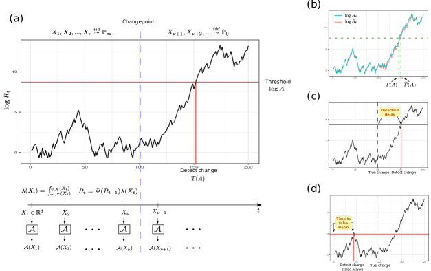
Figure 1: Overview of sequential changepoint detection in the classifier setting. (a) Data $X_{1},X_{2},...$ is observed from the pre-change distribution $\mathbb{P}_{\infty}$ and the post-change distribution $\mathbb{P}_{0}$. At each time $t$, a prediction $\mathcal{A}(X_{t})$ is made. If $f_{0,X}$ and $f_{\infty,X}$ are known, then a detection statistic $R_{t}$ can be calculated using the likelihood ratio $\lambda(X_{t})$. A change is detected when $R_{t}\geq A$ (or equivalently $\log R_{t}\geq\log A$). (b) When the true likelihood ratio $\lambda$ is unknown, we can use an estimate $\widehat{\lambda}$ instead; $\widetilde{R}_{t}=\Psi(\widetilde{R}_{t-1})\widehat{\lambda}(X_{t})$ is the resulting detection statistic. When $\widehat{\lambda}$ is close to $\lambda$, the stopping times $\widetilde{T}(A)$ and $T(A)$ are also expected to be close. (c) When a change is detected after the true changepoint $\nu$, then $T(A)-\nu$ is the detection delay. (d) When $T(A)<\nu$, then we have a false alarm, and $T(A)$ is the time to false alarm.

2.1 Problem statement and notation

We consider a sequential classification setting with unobserved labels, where feature vectors $X_{1},X_{2},X_{3},...\in\mathbb{R}^{d}$ arrive sequentially, but the associated labels $Y_{i}\in\{0,1\}$ are unobserved. In our dengue example, $X_{i}$ represents diagnostic measurements like temperature and white blood cell count, while $Y_{i}$ represents true dengue status. We assume that a classifier, $\mathcal{A}(\cdot)$, has been trained on a separate set of training observations $(X_{1}^{\prime},Y_{1}^{\prime}),...,(X_{m}^{\prime},Y_{m}^{\prime})$ and is used to predict the unobserved labels $Y_{i}$.

At some time $\nu\geq 0$ in this sequence, called the changepoint, the distribution of $(X_{i},Y_{i})$ changes. We notate the pre-change distribution as $\mathbb{P}_{\infty}$ and the post-change distribution as $\mathbb{P}_{0}$, such that $(X_{1}^{\prime},Y_{1}^{\prime})$,…,$(X_{m}^{\prime},Y_{m}^{\prime})$, $(X_{1},Y_{1})$,…,$(X_{\nu},Y_{\nu})\overset{iid}{\sim}\mathbb{P}_{\infty}$ and $(X_{\nu+1},Y_{\nu+1}),(X_{\nu+2},Y_{\nu+2}),...\overset{iid}{\sim}\mathbb{P}_{0}$. Our aim is to detect the change in the distribution of $(X_{i},Y_{i})$ as quickly as possible, using the observed sequence $X_{i}$.

Remark 1.

Throughout the paper we use the subscripts $\infty$ and 0 for pre- and post-change quantities respectively, to be consistent with the sequential changepoint detection literature. The motivation is that $\nu=\infty$ indicates the change never occurs, so data is from the pre-change distribution, while $\nu=0$ indicates the change occurs before we observe any data, so data is from the post-change distribution. When context is clear we will let $\mathbb{P}_{\infty}$ and $\mathbb{P}_{0}$ denote general pre- and post-change distributions, so for example $(X_{i},Y_{i})\sim\mathbb{P}_{\infty}$ and $X_{i}\sim\mathbb{P}_{\infty}$ both indicate data drawn before a change occurs.

The general problem of classification under a changed distribution has been studied extensively in the literature. Because arbitrary changes to high-dimensional classification data may be impossible to correct or detect, it is standard to make additional assumptions on the nature of the change. Because it frequently arises in practice, we will focus on the label shift setting (Saerens et al.,, 2002; Storkey,, 2009), which has received recent attention in the machine learning literature (Ackerman et al.,, 2020; Azizzadenesheli et al.,, 2019; Lipton et al.,, 2018; Rabanser et al.,, 2019). Label shift assumes that the marginal distribution of $Y_{i}$ changes, but the conditional distribution of $X_{i}|Y_{i}$ does not:

Definition 1 (Label shift).

Let $f_{\infty,X,Y}$, $f_{\infty,Y}$, and $f_{\infty,X|Y=y}$ denote the densities/mass functions of $(X,Y)$, $Y$, and $X|Y=y$ respectively, under $\mathbb{P}_{\infty}$. Similarly define $f_{0,X,Y}$, $f_{0,Y}$, and $f_{0,X|Y=y}$. The label shift assumption is that $f_{0,X|Y=y}\equiv f_{\infty,X|Y=y}$ for all $y$, so

$$f_{0,X,Y}(x,y)=f_{0,Y}(y)f_{0,X|Y=y}(x)=f_{0,Y}(y)f_{\infty,X|Y=y}(x)\hskip 28.45274pt\forall x,y.$$ (1)

Label shift is simply a change in the mixing proportion for the class distributions $X|Y=0$ and $X|Y=1$. Since the conditional distribution of $X|Y=y$ remains the same, the conditional distribution of the classifier predictions, $\mathcal{A}(X)|Y=y$, does as well. As we show in the following sections, the classifier predictions $\mathcal{A}(X_{i})$ can be further leveraged to improve changepoint detection in the label shift setting.

2.2 Proposed method

Let $(X_{1}^{\prime},Y_{1}^{\prime}),...,(X_{m}^{\prime},Y_{m}^{\prime})\overset{iid}{\sim}\mathbb{P}_{\infty}$ denote our labeled training set, used to train the classifier $\mathcal{A}(\cdot)$. Classifiers typically predict either the probability of a positive case $\mathbb{P}(Y_{i}=1|X_{i})$ or the label $Y_{i}$, and so we assume $\mathcal{A}(X_{i})\in[0,1]$ is a predicted probability, or $\mathcal{A}(X_{i})\in\{0,1\}$ is a predicted label.

To detect a change in the unlabeled sequence $X_{1},X_{2},...$, many changepoint detection procedures use a recursive detection statistic $R_{t}^{x}=\Psi(R_{t-1})\lambda(X_{t})$, where $\lambda(X_{t})=f_{0,X}(X_{t})/f_{\infty,X}(X_{t})$ is the likelihood ratio at time $t$, $\Psi$ is an update function, and the initial value is $R_{0}^{x}=x$ (Figure 1(a)). For example, the classical CUSUM procedure has $\Psi(r)=\max\{1,r\}$ and $x=1$, while the Shiryaev-Roberts procedure has $\Psi(r)=1+r$ and $x=0$ (Polunchenko and Tartakovsky,, 2012). A change is detected when $R_{t}^{x}$ crosses a pre-specified threshold $A>R_{0}^{x}$, with stopping time $T^{x}(A)=\inf\{t\geq 1:R_{t}^{x}\geq A\}$.

In most applications, $\lambda=f_{0,X}/f_{\infty,X}$ is unknown. However, under the label shift assumption, we can rewrite the likelihood ratio as

$$\frac{f_{0,X}(X_{i})}{f_{\infty,X}(X_{i})}=\left(\frac{\pi_{0}}{\pi_{\infty}}-\frac{1-\pi_{0}}{1-\pi_{\infty}}\right)\mathbb{P}_{\infty}(Y_{i}=1|X_{i})+\frac{1-\pi_{0}}{1-\pi_{\infty}},$$ (2)

with pre- and post-change proportions $\pi_{\infty}=\mathbb{P}_{\infty}(Y=1)$ and $\pi_{0}=\mathbb{P}_{0}(Y=1)$. Noting that $\mathbb{P}_{\infty}(Y=1|X=x)$ is a typical estimand in classification, we define the estimated likelihood ratio $\widehat{\lambda}_{\mathcal{A},m}$ by

$$\widehat{\lambda}_{\mathcal{A},m}(x)=\left(\frac{\pi_{0}}{\pi_{\infty}}-\frac{1-\pi_{0}}{1-\pi_{\infty}}\right)\mathcal{A}(x)+\frac{1-\pi_{0}}{1-\pi_{\infty}},$$ (3)

where the subscripts $\mathcal{A}$ and $m$ denote dependence on the classifier and the size of the training set. Our method detects label shift with the nonparametric detection statistic $\widetilde{R}_{t}^{x}$ and resulting stopping time $\widetilde{T}^{x}(A)$, where $\widetilde{R}_{0}^{x}=x$ and $\widetilde{R}_{t}^{x}=\Psi(\widetilde{R}_{t-1}^{x})\widehat{\lambda}_{\mathcal{A},m}(X_{t})$, and $\widetilde{T}^{x}(A)=\inf\{t\geq 1:\widetilde{R}_{t}^{x}\geq A\}$ (Figure 1(b)). When the pre- and post-change proportions $\pi_{\infty}$ and $\pi_{0}$ are known, performance of our label shift detection method depends on performance of the classifier $\mathcal{A}$, which we formalize in Section 3 and illustrate with simulations in Section 4. When $\pi_{0}$ is unknown, we use a mixing procedure that integrates (3) over possible values of $\pi_{0}$ (as we have access to labeled pre-change training data, the assumption that $\pi_{\infty}$ is known is reasonable). We discuss this mixing procedure in the following section.

Remark 2.

Using classifier predictions to estimate the likelihood ratio is natural in the label shift setting, as a classifier is already constructed and being applied to make predictions for new data. However, an advantage of the label shift setting is that it supports a variety of other approaches to likelihood ratio estimation. For example, approaches like kernel mean matching (Gretton et al.,, 2009) and uLSIF (Kanamori et al.,, 2009) rely on both pre- and post-change data; under the label shift assumption, a post-change sample can be generated by re-sampling or re-weighting the training data $(X_{1}^{\prime},Y_{1}^{\prime}),...,(X_{m}^{\prime},Y_{m}^{\prime})$ when $\pi_{0}$ is known. We compare this approach to our classifier-based likelihood ratio estimate in Section 4.

2.2.1 Changepoint detection with unknown $\pi_{0}$

As part of training our classifier $\mathcal{A}$, we have access to labeled pre-change training data
$(X_{1}^{\prime},Y_{1}^{\prime}),...,(X_{m}^{\prime},Y_{m}^{\prime})$, but it is less common to have a sample of post-change data, and so the post-change parameter $\pi_{0}$ is often unknown. To overcome an unknown $\pi_{0}$, we mix over a set $\Pi_{0}\subset[0,1]$ of potential values for the post-change parameter, with a weight distribution $w$. Here we are inspired by the work of Lai, (1998), which deals with the computational complexity involved in the integration by considering a window-limited approach that uses only a fixed number of the most recent observations. Let $\Pi_{0}$ be the set of possible values for $\pi_{0}$, and let $w(\pi_{0})$ be a density on $\Pi_{0}$. Each potential $\pi_{0}$ results in a different likelihood ratio function $\lambda_{\pi_{0}}$. Lai defines a CUSUM-type mixture stopping rule with detection statistic $R_{t,w}$ and stopping time $T_{w}(A)$ (Lai,, 1998):

$$R_{t,w}=\max\limits_{t-m_{\alpha}\leq k\leq t}\int\limits_{\Pi_{0}}\prod\limits_{i=k}^{t}\lambda_{\pi_{0}}(X_{i})w(\pi_{0})d\pi_{0}\hskip 28.45274ptT_{w}(A)=\inf\{t\geq 1:R_{t,w}\geq A\},$$ (4)

where $m_{\alpha}$ is the window size. In our label shift setting, we have

$$\lambda_{\pi_{0}}(x)=\frac{\pi_{0}f_{\infty,X|Y=1}(x)+(1-\pi_{0})f_{\infty,X|Y=0}(x)}{\pi_{\infty}f_{\infty,X|Y=1}(x)+(1-\pi_{\infty})f_{\infty,X|Y=0}(x)}.$$ (5)

For each $\pi_{0}$, we replace $\lambda_{\pi_{0}}$ with its estimate $\widehat{\lambda}_{\pi_{0},\mathcal{A},m}$ from (3), yielding the detection statistic $\widetilde{R}_{t,w}$ and stopping time $\widetilde{T}_{w}(A)$:

$$\widetilde{R}_{t,w}=\max\limits_{t-m_{\alpha}\leq k\leq t}\int\limits_{\Pi_{0}}\prod\limits_{i=k}^{t}\widehat{\lambda}_{\pi_{0},\mathcal{A},m}(X_{i})w(\pi_{0})d\pi_{0}\hskip 28.45274pt\widetilde{T}_{w}(A)=\inf\{t\geq 1:\widetilde{R}_{t,w}\geq A\}.$$ (6)

When $\mathcal{A}(X_{i})$ is a good estimate of $\mathbb{P}_{\infty}(Y_{i}=1|X_{i})$, we expect $\widetilde{T}_{w}(A)$ (6) to be close to $T_{w}(A)$ (4). We formalize this statement in Section 3.3, and we show that our estimated mixing procedure performs well on real dengue data in Section 5.

An alternative to mixing over $\Pi_{0}$ is to maximize over possible values of $\pi_{0}$ at each time step. This is the generalized likelihood ratio (GLR) approach, and has also been studied in previous research (see, e.g., Siegmund and Venkatraman, (1995)). For exponential families, some optimality properties of the GLR have been shown, but it is typically harder to control the average run length to false alarm (Tartakovsky et al.,, 2014). Another option is to perform detection with a worst-case $\pi_{0}^{*}\in\Pi_{0}$ (Unnikrishnan et al.,, 2011), which provides a worst-case bound on detection delay.

2.3 Background and related literature

2.3.1 Label shift testing

Non-sequential two-stample tests between training and test data have been proposed for detecting label shift between batches of data. Saerens et al., (2002) propose a likelihood ratio test, based on expectation-maximization. In Lipton et al., (2018), the authors note that label shift implies a change in the distribution of classifier predictions, and therefore use a two-sample test directly on the training and test set predictions to detecting the change. This is expanded by Rabanser et al., (2019), who recommend tests for label shift as a general method for detecting distributional changes, even if the label shift assumption is not met. For sequential detection of label shift, Ackerman et al., (2020) implement the nonparametric detection procedure in Ross and Adams, (2012) based on repeated Cramer–von-Mises tests for a change in distribution, using the cpm package (Ross,, 2015) in R. Like Ackerman et al., (2020), we consider the problem of detecting label shift in a sequential setting, rather than a batch setting. In the sequential setting, label shift detection is an example of the classic problem of sequential changepoint detection, and we apply nonparametric sequential detection tools to the label shift problem. In contrast to Ackerman et al., (2020), we use classifier predictions and the label shift assumption to directly approximate the likelihood ratio for sequential detection, which allows us to construct asymptotically optimal nonparametric label shift detection procedures.

2.3.2 Nonparametric detection procedures

Because the pre- and post-change data distributions are rarely known in practice, a variety of nonparametric detection procedures have been proposed. For example, several authors have adapted nonparametric hypothesis tests to the changepoint detection problem, such as Kolmogorov-Smirnov tests (Madrid Padilla et al.,, 2019), Cramer-von-Mises tests (Ross and Adams,, 2012), and graph-based nearest-neighbors tests (Chen,, 2019; Chu and Chen,, 2018). Another common approach is to replace the likelihood ratio $\lambda$ with an estimate $\widehat{\lambda}$. Often, this estimate $\widehat{\lambda}$ is constructed to detect specific types of expected changes, such as shifts in the mean or variance (Brodsky and Darkhovsky,, 1993, 2000; Tartakovsky et al., 2012b, ; Tartakovsky et al., 2006a, ; Tartakovsky et al., 2006b, ), or a change to a stochastically larger/smaller distribution (Bell et al.,, 1994; Gordon and Pollak,, 1994, 1995; McDonald,, 1990).

Other authors employ nonparametric density ratio estimates that utilize samples from both the pre- and post-change distributions $\mathbb{P}_{\infty}$ and $\mathbb{P}_{0}$. For example, Baron, (2000) estimates the post-change distribution sequentially with a histogram density estimator, while another approach is to choose the ratio that maximizes an estimate of the divergence between the pre- and post-change distributions (Nguyen et al.,, 2010; Kanamori et al.,, 2009; Kawahara and Sugiyama,, 2009; Sugiyama et al.,, 2008; Liu et al.,, 2013). Similarly, the kernel mean matching approach (Gretton et al.,, 2009; Yu and Szepesvári,, 2012) estimates the ratio by matching moments after mapping into a reproducing kernel Hilbert space (RKHS), while Bickel et al., (2009) propose training a classifier to predict whether data comes from the pre- or post-change distribution.

In the label shift case, the difficulty of having samples from the post-change distribution is reduced to knowing the post-change parameter $\pi_{0}$ (see (1)). In the following section, we propose a simple estimate of the likelihood ratio as a linear function of the classifier scores $\mathcal{A}(X_{i})$. An advantage of this method is that the existing classifier can be used without additional estimation, and performance of the detection procedure is directly related to performance of the classifier. In addition, when $\pi_{0}$ is unknown it is easy to calculate the likelihood ratio over a range of potential values $\Pi_{0}$, without having to re-estimate the ratio each time (see Section 2.2.1).

2.3.3 Operating characteristics

The performance of sequential detection procedures, with stopping time $T^{x}(A)$ at threshold $A$, is typically assessed by two operating characteristics, the average time to false alarm $\mathbb{E}_{\infty}(T^{x}(A))$ (also called the average run length, or ARL), and the average detection delay $\mathbb{E}_{0}(T^{x}(A))$, which are expected stopping times under the pre- and post-change distributions respectively (Figure 1(c) and 1(d)). The goal is to minimize the average detection delay, subject to a lower bound on the average time to false alarm, and the CUSUM and Shiryaev-Roberts procedures are known to be optimal or approximately optimal for this problem (Lorden,, 1971; Moustakides,, 1986; Tartakovsky et al., 2012a, ). We therefore compare average detection delay and average time to false alarm as a way to assess procedures in this manuscript.

3 Operating characteristics of nonparametric detection procedures

In Section 2.2, we introduced a nonparametric method for detecting label shift in sequential data. Our method relies on the classifier predictions $\mathcal{A}(X_{i})$, which can be used to directly estimate the likelihood ratio under the label shift assumption (see (3) and (6)). Our nonparametric procedure defines a stopping time $\widetilde{T}^{x}(A)$ (when the post-change proportion $\pi_{0}$ is known) or $\widetilde{T}_{w}(A)$ (when $\pi_{0}$ is unknown). Our stopping time is an approximation of the optimal stopping time $T^{x}(A)$ (or $T_{w}(A)$) which depends on the true likelihood ratio $\lambda=f_{0,X}/f_{\infty,X}$.

Naturally, we expect that the better $\mathcal{A}(x)$ estimates $\mathbb{P}_{\infty}(Y=1|X=x)$, the closer $\widetilde{T}^{x}(A)$ and $\widetilde{T}_{w}(A)$ are to $T^{x}(A)$ and $T_{w}(A)$. The purpose of this section is to formalize how detection performance depends on the classifier $\mathcal{A}$, which provides insight on the performance of our method and on selecting a classifier for changepoint detection. In Section 3.1, we define our measures of detection performance, based on convergence of expected stopping times. In Section 3.2, we provide conditions under which this convergence holds, and in Theorem 1 we give an upper bound on the rate of convergence which depends directly on the likelihood ratio estimate $\widehat{\lambda}$. Theorem 1 applies beyond the label shift setting to any estimate of the likelihood ratio, so we state it in generality and discuss our results in the context of label shift. For the special case of label shift, Theorem 1 requires $\pi_{0}$ to be known, and so we generalize our results to an unknown $\pi_{0}$ in Section 3.3. Finally, Theorem 1 assumes that $\mathcal{A}(X)$ is continuous, which occurs when $\mathcal{A}(x)\in[0,1]$ estimates $\mathbb{P}_{\infty}(Y=1|X=x)$. In Section 3.4, we describe conditions under which similar convergence results hold for binary classifiers $\mathcal{A}(X)\in\{0,1\}$. Examples illustrating our results are provided in Section 3.5.

3.1 Assessing performance of a nonparametric detection procedure

As discussed in Section 2.3, it is common to assess detection performance with the expected stopping times $\mathbb{E}_{\infty}(T)$ and $\mathbb{E}_{0}(T)$ under the pre- and post-change distributions. Previous results on the performance of nonparametric detection procedures have typically focused on the relative efficiency of estimated procedures compared to optimal performance (see, e.g., Bell et al., (1994); Unnikrishnan et al., (2011)), by examining the limiting behavior of the ratio $\mathbb{E}_{0}(\widetilde{T}^{x}(\widetilde{A}))/\mathbb{E}_{0}(T^{x}(A))$ as $\widetilde{A},A\to\infty$, where $\widetilde{A}$ is chosen so that $\mathbb{E}_{\infty}(\widetilde{T}^{x}(\widetilde{A}))=\mathbb{E}_{\infty}(T^{x}(A))$.

While relative efficiency is useful for comparing detection procedures, and it is natural to compare detection delay at the same average time to false alarm, formal results are typically asymptotic in the thresholds $A$ and $\widetilde{A}$. As an alternative, we consider a single fixed threshold $A$ and the differences $|\mathbb{E}_{i}(\widetilde{T}^{x}(A))-\mathbb{E}_{i}(T^{x}(A))|$, $i\in\{0,\infty\}$. To emphasize the dependence of $\mathbb{E}_{i}(\widetilde{T}^{x}(A))$ on $\widehat{\lambda}$, we will write $\mathbb{E}_{i}(\widetilde{T}^{x}(A)|\widehat{\lambda}_{m})$, where the subscript $m$ is used to show the dependence of $\widehat{\lambda}_{m}$ on the size of the training set. Ideally, $\mathbb{E}_{i}(\widetilde{T}^{x}(A)|\widehat{\lambda}_{m})\overset{p}{\to}\mathbb{E}_{i}(T^{x}(A))$ as $m\to\infty$. In the following sections, we provide conditions under which this convergence in probability holds, and we provide upper bounds on the rate of convergence.

3.2 Convergence for continuous likelihood ratios

We first consider the case when $\lambda(X)$ and $\widehat{\lambda}_{m}(X)$ are continuous, which is a common assumption in the changepoint detection literature. Under assumption (A1) - (A5) below, the convergence of $|\mathbb{E}_{i}(\widetilde{T}^{x}(A)|\widehat{\lambda}_{m})-\mathbb{E}_{i}(T^{x}(A))|$ depends on the total variation distance between the distributions of $\lambda(X)$ and $\widehat{\lambda}_{m}(X)$. Our main result is Theorem 1, which is not restricted to the label shift setting; let $\widehat{\lambda}_{m}$ be any likelihood ratio estimate from a training sample of size $m$ (not just (3)).

1. The detection procedure is defined by a detection statistic $R_{t}^{x}$ and a stopping time $T^{x}(A)=\inf\{t\geq 1:R_{t}^{x}\geq A\}$, with $R_{t}^{x}=\Psi(R_{t-1}^{x})\lambda(X_{t})$ and $R_{0}^{x}=x$. Likewise, the estimated detection procedure is defined by $\widetilde{T}^{x}(A)=\inf\{t\geq 1:\widetilde{R}_{t}^{x}(A)\geq A\}$, with $\widetilde{R}_{t}^{x}=\Psi(\widetilde{R}_{t-1}^{x})\widehat{\lambda}_{m}(X_{t})$ and $\widetilde{R}_{0}^{x}=x$.

2. The distributions of $\lambda(X)$ and $\widehat{\lambda}_{m}(X)$ are continuous, with $X\sim\mathbb{P}_{i}$.

3. The densities $f^{i}_{\lambda}$ and $f^{i}_{\widehat{\lambda}_{m}}$ of $\lambda(X)$ and $\widehat{\lambda}_{m}(X)$ under $\mathbb{P}_{i}$ satisfy the following assumptions:

   1. $\int\limits_{0}^{A}(f^{i}_{\lambda}(s))^{2}ds\ <\infty$ and $\int\limits_{0}^{A}(f^{i}_{\widehat{\lambda}_{m}}(s))^{2}ds\ <\infty$,

   2. $\lim\limits_{\varepsilon\to 0}\sup\limits_{x,z\in[0,A];|x-z|<\varepsilon}\int\limits_{0}^{A}|f^{i}_{\lambda}\left(\frac{y}{\Psi(x)}\right)-f^{i}_{\lambda}\left(\frac{y}{\Psi(z)}\right)|dy\ =0$ (and likewise for $f^{i}_{\widehat{\lambda}_{m}}$).

4. The functions $\Psi(r)$ and $1/\Psi(r)$ are Lipschitz continuous on $[0,A]$, and $\Psi(r)\geq 1$ for all $r$.

5. The total variation distance $TV(f^{i}_{\lambda},f^{i}_{\widehat{\lambda}_{m}})=\int|f^{i}_{\lambda}(s)-f^{i}_{\widehat{\lambda}_{m}}(s)|ds\ \overset{p}{\to}0$ as $m\to\infty$.

Assumption (A1) holds for standard detection procedures like CUSUM, Shiryaev-Roberts, and variants. Note that the assumption that $\lambda(X)$ is continuous is common in the changepoint detection literature, and is relied on by many approaches to calculating or approximating the expected stopping time of a detection procedure. In general we are interested in $|\mathbb{E}_{i}(\widetilde{T}^{x}(A)|\widehat{\lambda}_{m})-\mathbb{E}_{i}(T^{x}(A))|$ for both $i=0$ and $i=\infty$, which means (A2) requires $X$ is continuous and has the same support under $\mathbb{P}_{\infty}$ and $\mathbb{P}_{0}$, such as the ratio for two normal distributions (see Example 1 below). Assumption (A4) holds for common $\Psi$, such as $\Psi(r)=\max\{1,r\}$ (CUSUM) and $\Psi(r)=1+r$ (Shiryaev-Roberts). Assumption (A3) can be thought of as a requirement that the distributions of $\lambda(X)$ and $\widehat{\lambda}_{m}(X)$ are not close to having any point masses. A sufficient condition for (A3) is that the densities $f^{i}_{\lambda}$ and $f^{i}_{\widehat{\lambda}_{m}}$ are Lipschitz continuous.

Theorem 1.

Suppose that assumptions (A1) - (A5) hold. Then

$$|\mathbb{E}_{i}(\widetilde{T}^{x}(A)|\widehat{\lambda}_{m})-\mathbb{E}_{i}(T^{x}(A))|\leq O_{P}(TV(f^{i}_{\lambda},f^{i}_{\widehat{\lambda}_{m}})).$$ (7)

If, in addition, $f_{\lambda}^{i}$ is bounded, then

$$|\mathbb{E}_{i}(\widetilde{T}^{x}(A)|\widehat{\lambda}_{m})-\mathbb{E}_{i}(T^{x}(A))|\leq O_{P}(\mathbb{E}_{i}(|\widehat{\lambda}_{m}(X)-\lambda(X)|)+O_{P}(||F^{i}_{\widehat{\lambda}_{m}}-F^{i}_{\lambda}||_{\infty}).$$ (8)

Proof.

See the Supplementary Materials, Section A.2. ∎

3.2.1 Application to label shift

The estimate $\widehat{\lambda}_{\mathcal{A},m}$ from (3) can be reasonably assumed continuous when $\mathcal{A}(X)\in[0,1]$ is a predicted probability. The bound in Theorem 1 depends on the distribution of the likelihood ratio, which is intuitive as our detection procedure includes a random draw from this distribution at each step (see (A1)). As we can see from (8), when $f_{\lambda}^{i}$ is bounded, convergence depends directly on the $L_{1}$ rate of convergence of the likelihood ratio estimate $\widehat{\lambda}_{m}$. In the classifier setting, this is equivalent to the $L_{1}$ convergence of the classifier scores $\mathcal{A}(X)$ to the true probabilities $\mathbb{P}_{\infty}(Y=1|X)$, illustrating that performance of the changepoint detection procedure depends on performance of the classifier. If parametric assumptions are made, then we can expect parametric rates of convergence for the operating characteristics, as discussed in Example 1 and Example 2 below. Note that without parametric assumptions, the optimal $L_{1}$ rate of convergence is $m^{-p/(2p+d)}$ if $\lambda$ is a $p$-times differentiable function (Stone,, 1982), though not all classifiers will converge. In general, results for nonparametric regression are more common for $L_{2}$ convergence rather than $L_{1}$ convergence, and the same is true for other methods of density ratio estimation – for example, Nguyen et al., (2010) provide conditions under which a density ratio estimate from divergence maximization converges in Hellinger distance. Finally, note that convergence in (8) requires $\pi_{0}$ to be known for the estimate $\widehat{\lambda}_{\mathcal{A},m}$ from (3). In the next section, we focus specifically on the label shift setting and consider the situation where $\pi_{0}$ is unknown, to generalize convergence results to our mixture procedure in (6).

Remark 3.

Consider the classifier label shift setting, with unlabeled data, where the true likelihood ratio $\lambda(x)=f_{0,X}(x)/f_{\infty,X}(x)$ is given by (2). Suppose that $\lambda(X)$ is continuous, but we use a binary classifier with $\mathcal{A}(X)\in\{0,1\}$ (for example, by thresholding predicted probabilities), and estimate $\lambda$ with $\widehat{\lambda}_{\mathcal{A},m}$ as in (3). Because the binary predictions $\mathcal{A}(X)$ will never converge to the true probabilities $\mathbb{P}_{\infty}(Y=1|X)$, then $\mathbb{E}_{i}(\widetilde{T}^{x}(A)|\widehat{\lambda}_{\mathcal{A},m})$ won’t converge to $\mathbb{E}_{i}(T^{x}(A))$. Therefore, if $\mathbb{P}_{\infty}(Y=1|X)$ is expected to be a continuous function of $X$, it is better to use predicted probabilities, rather than binary predictions, for changepoint detection. Binary predictions are only suitable when the classes $X|Y=0$ and $X|Y=1$ are separable, as we discuss below in Section 3.4.

3.3 Convergence of label shift detection with unknown $\pi_{0}$

In the label shift setting, Theorem 1 applies when $\lambda(X)$ and $\widehat{\lambda}_{\mathcal{A},m}(X)$ are continuous, and $\pi_{0}$ is known or can be consistently estimated. However, as discussed in Section 2.2.1, we typically expect $\pi_{0}$ to be unknown in practice. Here we explicitly consider the classifier label shift setting, with likelihood ratio estimate $\widehat{\lambda}_{\pi_{0},\mathcal{A},m}$ for each potential $\pi_{0}$ given by (3). Note that an advantage of this likelihood ratio estimate is that mixing over $\Pi_{0}$ is simple: we need only change $\pi_{0}$ in (3). In contrast, two-sample ratio estimation procedures like those discussed in Gretton et al., (2009), Nguyen et al., (2010), and Kanamori et al., (2009) would require a new post-change sample and a new likelihood ratio estimate to be calculated for each $\pi_{0}$.

Since $\pi_{0}$ is unknown, we apply the CUSUM-type mixture stopping rule (6) discussed in Section 2.2.1. As $\widetilde{R}_{t,w}$ cannot be written recursively, the proof techniques of Theorem 1 do not apply, but it is still possible to show that $\mathbb{E}_{i}(\widetilde{T}_{w}(A)|\mathcal{A})$ is consistent for $\mathbb{E}_{i}(T_{w}(A))$ as $m\to\infty$, though we lose the ability to provide a rate of convergence:

Theorem 2.

Let $\Pi_{0}=[a,b]$ where $0<a\leq b<1$, and suppose there exist sets $\mathcal{S}_{c}$ indexed by $c>0$, such that $\mathcal{S}_{c_{1}}\subseteq\mathcal{S}_{c_{2}}$ when $c_{1}>c_{2}$, $\lim\limits_{c\to 0}\mathbb{P}_{i}(X\in\mathcal{S}_{c})=1$, and such that $\sup\limits_{\begin{subarray}{c}x\in\mathcal{S}_{c}\\ \pi_{0}\in\Pi_{0}\end{subarray}}|\widehat{\lambda}_{\pi_{0},\mathcal{A},m}(x)-\lambda_{\pi_{0}}(x)|\overset{p}{\to}0$ for all $c$. Furthermore, assume that $\mathbb{E}_{i}(T_{w}(A))$ is a continuous function of $A$. Then for all $A>0$, $\mathbb{E}_{i}(\widetilde{T}_{w}(A)|\mathcal{A})\overset{p}{\to}\mathbb{E}_{i}(T_{w}(A))$.

Proof.

See the Supplementary Materials, Section A.4. ∎

In practice, the mixture procedure in (6) often performs quite close to the procedure with estimated likelihood ratio (3), and performance improves when $\Pi_{0}$ can be narrowed. We will see in Section 5 that the mixture procedure outperforms other nonparametric detection procedures which don’t require knowledge of $\pi_{0}$ for detecting a change in dengue prevalence.

3.4 Label shift detection with binary predictions: separable class distributions

As discussed above, if $\lambda(X)$ is continuous then it makes sense to use predicted probabilities $\mathcal{A}(X)\in[0,1]$ to construct the likelihood ratio estimate $\widehat{\lambda}_{\mathcal{A},m}(X)$. However, it is common to use binary classifiers with $\mathcal{A}(X)\in\{0,1\}$. In this section, we provide a convergence result for label shift detection based on binary predictions, which depends on separable class distributions.

If $X|Y=0$ and $X|Y=1$ are separable, then optimal changepoint detection with the unlabeled data $X_{1},X_{2},X_{3},...$ is equivalent to optimal changepoint detection with the labeled data $(X_{1},Y_{1}),(X_{2},Y_{2}),(X_{3},Y_{3}),...$, with likelihood ratio

$$\frac{f_{0,X,Y}(X_{i},Y_{i})}{f_{\infty,X,Y}(X_{i},Y_{i})}=\left(\frac{\pi_{0}}{\pi_{\infty}}-\frac{1-\pi_{0}}{1-\pi_{\infty}}\right)Y_{i}+\frac{1-\pi_{0}}{1-\pi_{\infty}}.$$ (9)

Assuming the classifier $\mathcal{A}$ can separate the two classes given enough training data, then the nonparametric detection procedure is asymptotically optimal, and convergence of $|\mathbb{E}_{i}(\widetilde{T}^{x}(A)|\widehat{\lambda}_{m})-\mathbb{E}_{i}(T^{x}(A))|$ depends on the sensitivity and specificity of $\mathcal{A}$:

Corollary 1.

Suppose that $\pi_{\infty}$ and $\pi_{0}$ are known, and furthermore that $\log(\pi_{0}/\pi_{\infty})$ and $\log((1-\pi_{0})/(1-\pi_{\infty}))$ are rational. The optimal detection procedure observes $(X_{1},Y_{1}),(X_{2},Y_{2}),...$, with likelihood ratio $\lambda(X_{i},Y_{i})$ given by (9), and detection statistic $R_{t}^{x}=\max\{1,R_{t-1}^{x}\}\lambda(X_{t},Y_{t})$. When the labels $Y_{i}$ are unobserved, the nonparametric detection procedure uses a binary classifier $\mathcal{A}$, with $\mathcal{A}(X)\in\{0,1\}$; the likelihood ratio $\widehat{\lambda}_{\mathcal{A},m}$ is given by (3), and the detection statistic is $\widetilde{R}_{t}^{x}=\max\{1,\widetilde{R}_{t-1}^{x}\}\widehat{\lambda}_{\mathcal{A},m}(X_{t})$. Then, if $\mathbb{P}_{i}(\mathcal{A}(X)=1|Y=1,\mathcal{A})\overset{p}{\to}1$ and $\mathbb{P}_{i}(\mathcal{A}(X)=0|Y=0,\mathcal{A})\overset{p}{\to}1$ as $m\to\infty$,

$$|\mathbb{E}_{i}(\widetilde{T}^{x}(A)|\widehat{\lambda}_{m})-\mathbb{E}_{i}(T^{x}(A))|\leq O_{P}(\mathbb{P}_{i}(\mathcal{A}(X)=0|Y=1,\mathcal{A})+\mathbb{P}_{i}(\mathcal{A}(X)=1|Y=0,\mathcal{A})).$$ (10)

Proof.

See the Supplementary Materials, Section A.3. ∎

The detection procedure in Corollary 1 is simply a Bernoulli CUSUM procedure, and the right hand side of (10) depends on the convergence of the specificity and sensitivity of the classifier $\mathcal{A}$, which requires that the two distributions $X|Y=0$ and $X|Y=1$ can be separated. This is a stronger requirement than in Theorem 1: consistently estimating probabilities $\mathbb{P}_{i}(Y=1|X)$ can be possible even when consistently estimating labels is impossible. In practice, $X|Y=0$ and $X|Y=1$ are rarely perfectly separable, but Corollary 1 is still helpful for seeing the relationship between classifier performance and changepoint performance.

The assumption that $\log(\pi_{0}/\pi_{\infty})$ and $\log((1-\pi_{0})/(1-\pi_{\infty}))$ are rational is needed to ensure that $R_{t}^{x}$ and $\widetilde{R}_{t}^{x}$ are Markov processes on the same state space, as is the restriction of $\Psi$ to the CUSUM $\Psi(x)=\max\{1,x\}$. In practice, Reynolds Jr and Stoumbos, (1999) show that the expected stopping time is close when $\log\lambda(X)$ is not rational but a rational approximation is used.

3.5 Examples

To help illustrate our theoretical results, we consider several specific change detection scenarios, which provide concrete examples of our results in action. First, we consider a simple univariate parametric setting. When we have a parametric model, we hope that the rate of convergence for our detection procedure is the same as the rate of convergence for the parameter estimates. In this example, we consider a shift in the mean of a normal distribution, which also demonstrates that our results extend beyond the label shift setting.

Example 1 (Gaussian mean shift).

Suppose it is known that under $\mathbb{P}_{\infty}$, $X\sim N(0,1)$, and under $\mathbb{P}_{0}$, $X\sim N(\mu,1)$, with $\mu>0$. Then, the likelihood ratio $\lambda$ is given by $\lambda(x)=\exp\{\mu x-\mu^{2}/2\}$. Furthermore, we have a training sample $X_{1}^{\prime},...,X_{m}^{\prime}\overset{iid}{\sim}N(\mu,1)$, with which we estimate $\mu$ by $\widehat{\mu}_{m}=\frac{1}{m}\sum\limits_{i=1}^{m}X_{i}^{\prime}$; the likelihood ratio estimate is then $\widehat{\lambda}_{m}(x)=\exp\{\widehat{\mu}_{m}x-\widehat{\mu}_{m}^{2}/2\}$ (this is similar to the procedures proposed in Tartakovsky et al., 2012b ). Then, the conditions for Theorem 1 hold with $TV(f^{i}_{\lambda},f^{i}_{\widehat{\lambda}_{m}})\leq O_{P}(|\widehat{\mu}_{m}-\mu|)$. Therefore, an upper bound on the rate of convergence for the estimated detection procedure is $|\mathbb{E}_{i}(\widetilde{T}^{x}(A)|\widehat{\lambda}_{m})-\mathbb{E}_{i}(T^{x}(A))|\leq O_{P}(|\widehat{\mu}_{m}-\mu|)=O_{P}(1/\sqrt{m})$. Full details and calculations can be found in the Supplementary Materials (A.5).

We now examine the case where we detect label shift with classifier predictions. To make the example clear, we consider a linear discriminant analysis (LDA) classifier, for which the classifier scores and their distribution have a closed form.

Example 2 (LDA).

Suppose that under $\mathbb{P}_{\infty}$, $X\sim\pi_{\infty}N(\bm{\mu}_{1},\bm{\Sigma})+(1-\pi_{\infty})N(\bm{\mu}_{0},\bm{\Sigma})$, while under $\mathbb{P}_{0}$, $X\sim\pi_{0}N(\bm{\mu}_{1},\bm{\Sigma})+(1-\pi_{0})N(\bm{\mu}_{0},\bm{\Sigma})$. Suppose that $\pi_{\infty}$ and $\pi_{0}$ are known, and we have a training sample $X_{1}^{\prime},...,X_{m}^{\prime}\overset{iid}{\sim}\mathbb{P}_{\infty}$ with which we construct estimates $\widehat{\bm{\mu}}_{1},\widehat{\bm{\mu}}_{0},\widehat{\bm{\Sigma}}$. Our likelihood ratio estimate $\widehat{\lambda}_{\mathcal{A},m}$ is given by (3), where $\mathcal{A}$ is given by

$$\mathcal{A}(X_{i})=\frac{\pi_{\infty}\mathrm{MVN}(X_{i};\widehat{\bm{\mu_{1}}},\widehat{\bm{\Sigma}})}{\pi_{\infty}\mathrm{MVN}(X_{i};\widehat{\bm{\mu_{1}}},\widehat{\bm{\Sigma}})+(1-\pi_{\infty})\mathrm{MVN}(X_{i};\widehat{\bm{\mu_{0}}},\widehat{\bm{\Sigma}})},$$ (11)

where $\mathrm{MVN}(\cdot;\bm{\mu},\bm{\Sigma})$ denotes the multivariate normal density with mean $\bm{\mu}$ and covariance matrix $\bm{\Sigma}$. The true likelihood ratio is similar, just replacing $\widehat{\bm{\mu}}_{1},\widehat{\bm{\mu}}_{0},\widehat{\bm{\Sigma}}$ with the true parameters. (A3) follows because $f^{i}_{\lambda}$ and $f^{i}_{\widehat{\lambda}}$ can be shown to be Lipschitz, while (A5) follows from the strong consistency of $\widehat{\bm{\mu}}_{i}$ and $\widehat{\bm{\Sigma}}$. The rate of convergence in Theorem 1 depends on the rate of convergence for $||\widehat{\bm{\Sigma}}^{-1}-\bm{\Sigma}^{-1}||_{F}$, where $||\cdot||_{F}$ denotes Frobenius norm. Details are provided in the Supplementary Materials (A.6).

While the formal results in Theorem 1 and Corollary 1 depend on convergence of $\widehat{\lambda}(X)$ to $\lambda(X)$, detection performance will depend on classifier performance even if $\widehat{\lambda}(X)$ does not converge. Here we demonstrate that the relationship between detection delay and classifier performance still holds for mis-specified classifiers, and that the expected $L_{1}$ distance from Theorem 1, $\mathbb{E}_{i}(|\widehat{\lambda}(X)-\lambda(X)|)$, is a useful summary of classifier performance.

Example 3 (LDA vs. QDA).

Suppose we observe training data $(X_{1}^{\prime},Y_{1}^{\prime}),...,(X_{m}^{\prime},Y_{m}^{\prime})\in\mathbb{R}^{150}$, with $X|Y=0\sim N(\bm{\mu_{0}},\bm{\Sigma_{0}})$ and $X|Y=1\sim N(\bm{\mu_{1}},\bm{\Sigma_{1}})$, with $\bm{\Sigma_{0}}\neq\bm{\Sigma_{1}}$. Construct linear discriminant analysis (LDA) and quadratic discriminant analysis (QDA) classifiers $\mathcal{A}_{L}$ and $\mathcal{A}_{Q}$. Using (3), perform CUSUM changepoint detection with each classifier. Figure 2 shows $\mathbb{E}_{0}(|\widehat{\lambda}(X)-\lambda(X)|)$ and $\mathbb{E}_{0}(\widetilde{T}(A))$ for the resulting LDA and QDA detection procedures; for each classifier, the threshold $A$ is chosen so that $\mathbb{E}_{\infty}(\widetilde{T}(A))\approx 180$. For large $m$, $\mathcal{A}_{Q}$ outperforms $\mathcal{A}_{L}$ because the QDA assumptions are met whereas the LDA assumptions are violated, but for small $m$ we see that $\mathcal{A}_{L}$ does better due to the bias-variance trade-off. As shown in Figure 2, the LDA detection procedure does better than the QDA detection procedure exactly when $\mathcal{A}_{L}$ outperforms $\mathcal{A}_{Q}$.

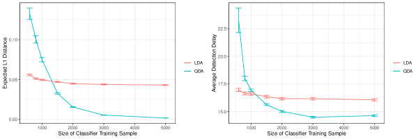
Figure 2: Comparison between changepoint detection with LDA and QDA classifier scores, when LDA assumptions are violated but QDA assumptions are satisfied. Left: Average L1 distance of the likelihood ratio estimate, as a function of the size of the classifier training sample. Right: Each LDA and QDA classifier is used for changepoint detection with the classifier scores. This plot shows the average detection delay when the average ARL is approximately 180 (averaged across classifiers) as a function of the size of the classifier training sample.

In Example 2, we used an LDA classifier to detect label shift in a mixture of normals with a common covariance matrix. Here we consider a similar procedure which uses nonparametric density estimation rather than an assumption of Gaussianity (see, e.g. Cipolli and Hanson, (2017, 2019)).

Example 4 (Density Estimation Classifier).

Suppose that $\pi_{\infty}$ and $\pi_{0}$ are known, and we have a training sample $X_{1}^{\prime},...,X_{m}^{\prime}\overset{iid}{\sim}\mathbb{P}_{\infty}$ with which we construct density estimates $\widehat{f}_{\infty,X|Y=0}$ and $\widehat{f}_{\infty,X|Y=1}$. Our classifier $\mathcal{A}$ is given by

$$\mathcal{A}(x)=\frac{\pi_{\infty}\widehat{f}_{\infty,X|Y=1}(x)}{\pi_{\infty}\widehat{f}_{\infty,X|Y=1}(x)+(1-\pi_{\infty})\widehat{f}_{\infty,X|Y=0}(x)},$$ (12)

and our likelihood ratio estimate is given by (3). For $c>0$, let $\mathcal{S}_{c}=\{x:f_{\infty,X}(x)>c\}$. Clearly, $\lim\limits_{c\to 0}\mathbb{P}_{i}(X\in\mathcal{S}_{c})=1$. Furthermore, with appropriate choice of kernel and bandwidth, $||\widehat{f}_{\infty,X|Y=1}-f_{\infty,X|Y=1}||_{\infty},||\widehat{f}_{\infty,X|Y=0}-f_{\infty,X|Y=0}||_{\infty}\overset{p}{\to}0$ (see, e.g., Giné and Guillou, (2002)). Thus for each $c$, $\sup\limits_{\begin{subarray}{c}x\in\mathcal{S}_{c}\\ \pi_{0}\in\Pi_{0}\end{subarray}}|\widehat{\lambda}_{\pi_{0},\mathcal{A},m}(x)-\lambda_{\pi_{0}}(x)|\overset{p}{\to}0$.

4 Simulation studies

We investigate the empirical performance of the classifier-based label shift detection procedure described in Section 2.2, with the likelihood ratio estimate in (3). Our likelihood ratio estimate depends on a classifier, and for simplicity we will use an LDA classifier, since it is easy to control whether the LDA assumptions are satisfied, as in Example 3. For comparison, we consider several other detection procedures, which represent different approaches to changepoint detection. These procedures are summarized below and in Table 1. Because the proposed procedure from Section 2.2 is designed specifically for the classifier label shift setting, it leverages more information than the other nonparametric detection procedures. In particular, as summarized in Table 1, estimating the likelihood ratio with (3) assumes that the label shift assumption holds, and the classifier $\mathcal{A}(\cdot)$ performs well. Through simulations, we show that detection with (3) outperforms the other nonparametric procedures when these assumptions are met, and can still perform well when the assumptions are violated. While we use a simple setting for simulations, in Section 5 we apply the same methods to detect a change in dengue prevalence using the data and classifier from Tuan et al., (2015), with similar results to our simulations in this section.

We compare the following methods:

Classifier-based CUSUM

This is the nonparametric method proposed in Section 2.2, with likelihood ratio estimate (3). For the purposes of simulations, $\mathcal{A}$ in (3) is an LDA classifier. Here we use a CUSUM procedure, so $\Psi(r)=\max\{1,r\}$.

Optimal CUSUM

The optimal CUSUM procedure (Page,, 1954) uses the true likelihood ratio, and can be implemented when the true likelihood ratio is known.

uLSIF CUSUM

uLSIF (Kanamori et al.,, 2009) is a nonparametric method for estimating the likelihood ratio, by maximizing an empirical divergence. As described in Section 2.2, uLSIF can be used with training data under the label shift assumption by re-weighting or re-sampling training points, but it does not exploit the label shift structure of the likelihood ratio. A variety of similar density ratio estimation approaches exist, including KLIEP and kernel mean matching (Sugiyama et al.,, 2008; Gretton et al.,, 2009; Kanamori et al.,, 2012), and we take uLSIF as a representative. Here we used the densratio package (Makiyama,, 2019) to implement uLSIF, and employ the resulting estimate in a CUSUM procedure.

CPM

Ackerman et al., (2020) perform nonparametric label shift detection using the CPM framework described in Ross et al., (2011) and Ross, (2015). The CPM framework detects changes in a sequence of univariate data using repeated nonparametric tests; Ackerman et al., (2020) applied repeated Cramer–von-Mises tests to a sequence of cosine divergences calculated between new data and training data. We evaluate CPM applied to both the classifier predictions and the cosine divergences used by Ackerman et al., (2020). CPM stopping times are calculated with the cpm package (Ross,, 2015).

kNN

Chen, (2019) and Chu and Chen, (2018) propose a sequential graph-based $k$-nearest neighbors (kNN) detection procedure, based on repeated nearest-neighbor two-sample tests in a sliding window. Note that while the kNN approach uses training data, only a fixed window of data is considered. Similar to some parameters in Chu and Chen, (2018), we set the window size to 200 and the number of nearest neighbors to $k=5$. Stopping times are calculated with the gStream package (Chen and Chu,, 2019).

Table 1: Comparison of the information used by each changepoint detection procedure considered in simulations. CPM and kNN are more general than the classifier CUSUM procedure from Section 2.2, but as a result they leverage less information. If the label shift assumption holds and the classifier performs well, we expect the classifier-based CUSUM method to outperform these more general procedures.

Information leveraged	Classifier CUSUM	Optimal CUSUM	uLSIF CUSUM	CPM (classifier)	CPM (divergence)	kNN
True labels		$\checkmark$
Label shift	$\checkmark$		$\checkmark$
Good classifier	$\checkmark$			$\checkmark$
Training data	$\checkmark$		$\checkmark$	$\checkmark$	$\checkmark$	$\checkmark$

4.1 Metrics

Performance of each detection procedure is measured by detection delay, calculated as $\mathbb{E}_{0}[T]$ (for CUSUM procedures, this corresponds to Lorden’s (Lorden,, 1971) detection delay). As is standard, we compare detection delays with each method calibrated to have the same average run length $\mathbb{E}_{\infty}[T]$. Here we use $\mathbb{E}_{\infty}[T]=500$, which is a common value in the sequential detection literature. Expected stopping times are estimated via Monte Carlo simulation.

4.2 Scenarios

Under the label shift assumption, the classifier-based CUSUM procedure uses classifier predictions $\mathcal{A}(X_{i})$ to estimate the likelihood ratio. To compare performance of the different detection procedures, we use two different simulation scenarios. In the first scenario, we change the training sample size and the performance of the classifier (by changing the distribution of the data $X_{i}$ and violating LDA assumptions). In the second scenario, we change the performance of the classifier and the suitability of the label shift assumption.

Scenario 1:

Pre-change data is generated as $X\sim\pi_{\infty}N(\bm{\mu_{1}},\bm{\Sigma_{1}})+(1-\pi_{\infty})N(\bm{\mu_{0}},\bm{\Sigma_{0}})$, and post-change data is generated as $X\sim\pi_{0}N(\bm{\mu_{1}},\bm{\Sigma_{1}})+(1-\pi_{0})N(\bm{\mu_{0}},\bm{\Sigma_{0}})$. In all simulations, $\pi_{\infty}=0.4$, $\pi_{0}=0.7$, $\bm{\mu_{0}}=[0,0]$, $\bm{\mu_{1}}=[1.5,1.5]$, and $\bm{\Sigma_{0}}=\bm{I}$. Training data $(X_{1}^{\prime},Y_{1}^{\prime}),...,(X_{m}^{\prime},Y_{m}^{\prime})$ is simulated from the pre-change distribution, and used to train the LDA classifier, estimate the uLSIF likelihood ratio, and startup the CPM and kNN detection statistics. We consider $m\in\{200,1000,5000\}$, and $\bm{\Sigma_{1}}\in\left\{\bm{I},\begin{bmatrix}2&0.1\\ 0.1&2\end{bmatrix},\begin{bmatrix}4&0.5\\ 0.5&4\end{bmatrix}\right\}$.

Scenario 2:

Pre-change data is generated as $X\sim\pi_{\infty}N(\bm{\mu_{\infty,1}},\bm{\Sigma_{1}})+(1-\pi_{\infty})N(\bm{\mu_{\infty,0}},\bm{\Sigma_{0}})$, and post-change data is generated as $X\sim\pi_{0}N(\bm{\mu_{0,1}},\bm{\Sigma_{1}})+(1-\pi_{0})N(\bm{\mu_{0,0}},\bm{\Sigma_{0}})$. In all simulations, $\pi_{\infty}=0.4$, $\pi_{0}=0.7$, $\bm{\mu_{\infty,0}}=[0,0]$, $\bm{\mu_{\infty,1}}=[1.5,1.5]$, and $\bm{\Sigma_{0}}=\bm{I}$. Training data $(X_{1}^{\prime},Y_{1}^{\prime}),...,(X_{1000}^{\prime},Y_{1000}^{\prime})$ is simulated from the pre-change distribution, and used to train the LDA classifier, estimate the uLSIF likelihood ratio, and startup the CPM and kNN detection statistics. We consider $\bm{\Sigma_{1}}\in\left\{\bm{I},\begin{bmatrix}2&0.1\\ 0.1&2\end{bmatrix},\begin{bmatrix}4&0.5\\ 0.5&4\end{bmatrix}\right\}$ and the following pairs for $\bm{\mu_{0,0}}$ and $\bm{\mu_{0,1}}$: $\bm{\mu_{0,0}}=[0.5,0.5]$ and $\bm{\mu_{0,1}}=[1,1]$; $\bm{\mu_{0,0}}=[0.75,0.75]$ and $\bm{\mu_{0,1}}=[0.75,0.75]$; and $\bm{\mu_{0,0}}=[1,1]$ and $\bm{\mu_{0,1}}=[0.5,0.5]$.

4.3 Results

Table 2 shows the results for Scenario 1, when the label shift assumption holds. We can see that when the LDA assumptions are met (specifically $\bm{\Sigma_{1}}=\bm{\Sigma_{0}}=\bm{I}$), LDA performs very close to the optimal CUSUM procedure, as we would predict from Example 2. Performance of the LDA detection procedure relative to the optimal CUSUM procedure declines as the assumption that $\bm{\Sigma_{1}}=\bm{\Sigma_{0}}$ is violated, but is still better than the other nonparametric methods. This suggests that if the label shift assumption holds, the likelihood ratio estimate in (3) is a good choice for detecting the change. Detection with the uLSIF procedure improves with training sample size $m$, as it becomes easier to estimate the likelihood ratio function and variability in the likelihood ratio estimate decreases. CPM also performs better as the sample size increases, as training data is used to construct the detection statistic. While the kNN method makes no assumptions about the change or the distribution of data, the cost of this flexibility is a decrease in detection performance.

Table 2: Simulation results for Scenario 1. Performance of each procedure is measured by detection delay, calculated as $\mathbb{E}_{0}[T]$. The estimated detection delay from Monte Carlo simulation is reported, with the standard error in parentheses. For the kNN procedure, a window of size 200 is used, so only 200 training points are considered. In the case of kNN, if a change is not detected within the sliding window, windows after time point 200 will consist of only post-change observations, so for computational purposes a fixed number of post-change observations is simulated and we report a lower bound on the detection delay.

$\bm{\Sigma_{1}}$	$m$	Detection delay when $\mathbb{E}_{\infty}[T]\approx 500$
		Classifier CUSUM	Optimal CUSUM	uLSIF CUSUM	CPM (classifier)	CPM (divergence)	kNN
$\begin{bmatrix}1&0\\ 0&1\end{bmatrix}$	200	28.8 (0.59)	29.0 (0.23)	33.8 (5.62)	46.9 (1.45)	51.5 (1.72)	$\geq 155$ (3.46)
	1000	28.8 (0.26)		33.4 (1.51)	35.0 (0.81)	37.0 (0.85)
	5000	28.8 (0.10)		31.5 (1.11)	32.6 (0.76)	33.7 (0.81)
$\begin{bmatrix}2&0.1\\ 0.1&2\end{bmatrix}$	200	34.3 (0.96)	33.1 (0.28)	49.0 (11.4)	61.2 (2.24)	69.5 (2.67)	$\geq 168$ (3.58)
	1000	34.0 (0.40)		43.3 (2.39)	42.4 (1.07)	46.6 (1.18)
	5000	34.0 (0.16)		38.8 (2.44)	38.1 (0.94)	41.7 (1.03)
$\begin{bmatrix}4&0.5\\ 0.5&4\end{bmatrix}$	200	41.9 (1.44)	33.4 (0.29)	164 (47.3)	74.6 (2.82)	94.8 (3.56)	$\geq 176$ (3.59)
	1000	41.8 (0.60)		73.3 (7.05)	52.1 (1.46)	62.4 (1.74)
	5000	41.9 (0.25)		54.2 (5.19)	51.2 (1.36)	58.5 (1.55)

Table 3 shows the results for Scenario 2, when the label shift assumption is violated. When the label shift assumption is approximately true ($\bm{\mu_{0,0}}=[0.5,0.5]$ and $\bm{\mu_{0,1}}=[1,1]$), we can see that LDA detection is comparable to uLSIF and CPM. However, the LDA procedure is more sensitive to large departures from the label shift assumption, for which methods with fewer assumptions perform better. Overall, CPM with classifier predictions performs well, as the classifier predictions are a useful summary of the data even when label shift doesn’t hold.

Table 3: Simulation results for Scenario 2. Performance of each procedure is measured by detection delay, calculated as $\mathbb{E}_{0}[T]$. The estimated detection delay from Monte Carlo simulation is reported, with the standard error in parentheses. For the kNN procedure, a window of size $200$ is used, so only 200 training points are considered. In the case of kNN, if a change is not detected within the sliding window, windows after time point 200 will consist of only post-change observations, so for computational purposes a fixed number of post-change observations is simulated and we report a lower bound on the detection delay.

$\bm{\Sigma_{1}}$	Post-change distribution	Detection delay when $\mathbb{E}_{\infty}[T]\approx 500$
		Classifier CUSUM	Optimal CUSUM	uLSIF CUSUM	CPM (classifier)	CPM (divergence)	kNN
$\begin{bmatrix}1&0\\ 0&1\end{bmatrix}$	$\!\begin{aligned} \bm{\mu_{0,0}}&=[0.5,0.5]\\ \bm{\mu_{0,1}}&=[1,1]\end{aligned}$	70.2 (1.68)	24.1 (0.17)	55.8 (4.49)	64.4 (1.27)	66.4 (1.40)	$\geq 130$ (3.22)
	$\!\begin{aligned} \bm{\mu_{0,0}}&=[0.75,0.75]\\ \bm{\mu_{0,1}}&=[0.75,0.75]\end{aligned}$	184 (7.49)	22.9 (0.16)	117 (14.6)	92.1 (1.64)	96.0 (1.78)	$\geq 131$ (3.30)
	$\!\begin{aligned} \bm{\mu_{0,0}}&=[1,1]\\ \bm{\mu_{0,1}}&=[0.5,0.5]\end{aligned}$	541 (17.4)	28.9 (0.21)	282 (3.23)	177 (3.18)	193 (3.55)	$\geq 161$ (3.57)
$\begin{bmatrix}2&0.1\\ 0.1&2\end{bmatrix}$	$\!\begin{aligned} \bm{\mu_{0,0}}&=[0.5,0.5]\\ \bm{\mu_{0,1}}&=[1,1]\end{aligned}$	70.9 (1.66)	34.3 (0.27)	67.9 (6.17)	74.6 (1.78)	79.4 (1.92)	$\geq 173$ (3.60)
	$\!\begin{aligned} \bm{\mu_{0,0}}&=[0.75,0.75]\\ \bm{\mu_{0,1}}&=[0.75,0.75]\end{aligned}$	123 (3.82)	31.4 (0.26)	101 (11.5)	109 (2.69)	120 (3.03)	$\geq 177$ (3.59)
	$\!\begin{aligned} \bm{\mu_{0,0}}&=[1,1]\\ \bm{\mu_{0,1}}&=[0.5,0.5]\end{aligned}$	225 (8.56)	30.0 (0.24)	166 (20.4)	196 (5.42)	217 (6.15)	$\geq 177$ (3.60)
$\begin{bmatrix}4&0.5\\ 0.5&4\end{bmatrix}$	$\!\begin{aligned} \bm{\mu_{0,0}}&=[0.5,0.5]\\ \bm{\mu_{0,1}}&=[1,1]\end{aligned}$	73.8 (1.67)	29.8 (0.24)	87.6 (10.1)	77.0 (1.98)	88.7 (2.49)	$\geq 170$ (3.57)
	$\!\begin{aligned} \bm{\mu_{0,0}}&=[0.75,0.75]\\ \bm{\mu_{0,1}}&=[0.75,0.75]\end{aligned}$	103 (2.78)	22.9 (0.19)	101 (11.9)	88.9 (2.55)	101 (3.08)	$\geq 152$ (3.50)
	$\!\begin{aligned} \bm{\mu_{0,0}}&=[1,1]\\ \bm{\mu_{0,1}}&=[0.5,0.5]\end{aligned}$	146 (4.58)	18.1 (0.15)	120 (15.3)	107 (3.12)	122 (3.75)	$\geq 120$ (3.20)

5 Detecting a change in dengue prevalence

We apply our changepoint detection procedure to the problem of detecting a change in the prevalence of dengue, using data and classifier predictions from the work of Tuan et al., (2015). As the prevalence of dengue changes, but the symptoms are expected to stay the same, the label shift assumption is appropriate for this change.

5.1 Data

Data comes from Tuan et al., (2015), who collected information on 5720 febrile patients aged 15 or younger in three Vietnamese hospitals. Of these patients, 30% had dengue. The authors recorded their true dengue status (using a gold-standard test), the results of an NS1 rapid antigen test, and a variety of physical measurements for classification with a logistic regression classifier.

5.2 Classifier

We use 1000 patients as training data for the classifier, and save the rest for evaluating our classifier and estimating changepoint detection performance. With the training set, we construct a logistic GAM classifier to predict true dengue status with the following covariates: vomiting (yes/no), skin bleeding (yes/no), BMI, age, temperature, white blood cell count, hematocrit, and platelet count. As in Tuan et al., (2015), the ROC curve has an AUC of approximately 0.8.

5.3 Scenarios

To assess change detection, we simulate a change in the prevalence of dengue by resampling the 4720 patients not used for training. As the group of patients in the study aims to represent the population of patients who would be tested for dengue, we take the sample proportion of 30% as our baseline dengue prevalence among patients who would be tested. The degree of change in this prevalence, when an outbreak occurs, depends on the magnitude of the outbreak and the baseline prevalence in the population. Magnitude of change varies; for example, Hanoi, Vietnam saw roughly a five-fold increase in 2009 and 2015 (Cuong et al.,, 2011; Cheng et al.,, 2020), while Kaohsiung City, Taiwan saw a 15-fold increase in 2014 (Hsu et al.,, 2017). Baseline prevalence in the full population varies depending on location – for example, Wiwanitkit, (2006) shows approximately 1 in 1 million for certain areas of Thailand, whereas Hsu et al., (2017) show roughly 1 in 10000 on average in Taiwan. For Vietnam, Cuong et al., (2011) report roughly 1 in 10000 to 1 in 1000 in Hanoi, with a peak of 384 per 100000 in 2009. For our purposes, we consider two label shift changes in prevalence:

Abrupt change:

We simulate an abrupt 5-fold increase, and take the baseline prevalence in the population to be roughly 1 in 10000. Applying Bayes rule, this gives a post-change prevalence of about 68% in our study population, and so we simulate a change from 30% to 68% and assess our ability to detect this shift.

Gradual change:

When the change occurs, prevalence increases gradually, rather than abruptly. Here, prevalence in the study population changes smoothly from 30% to 68% over the course of 100 observations.

5.4 Methods for comparison in dengue setting

We compare the methods from Section 4 to detect the change in dengue prevalence. The classifier CUSUM detection procedure is implemented using (3) with $\mathcal{A}(X)$ the predicted probabilities from the dengue classifier described above. We also compare CUSUM with binarized predictions, using both a threshold of 0.5 and the threshold, 0.33, which maximizes sensitivity + specificity. The optimal CUSUM procedure uses the true dengue status, which is observable if gold-standard tests are available, and we also include CUSUM with binary predictions from the NS1 rapid antigen tests, which again may not be available. The rapid test has a specificity of approximately 99% and a sensitivity of 70% (Tuan et al.,, 2015), compared with a specificity and sensitivity of 82% and 70% for the binarized classifier at threshold 0.33. As in Section 4, we also compare CPM using the classifier predicted probabilities, and CPM with divergences. uLSIF was considered but failed to consistently estimate the likelihood ratio, while kNN was not considered because it performed worse than the other methods in Section 4. Finally, as the post-change parameter is typically unknown, we include the mixing procedure described in (6). We use $\Pi_{0}=[0.6,0.8]$, which corresponds to a 3.5-fold to 9-fold increase in prevalence.

For the abrupt change scenario, all methods are compared. For the gradual change, we compare the mixture CUSUM procedure to CPM with classifier predictions, as these two methods perform well at detecting an abrupt change and do not require knowledge of the post-change parameter, and we include optimal CUSUM for reference.

Table 4: Comparison of method performance for detecting an abrupt change in dengue prevalence. Performance of each procedure is assessed by average detection delay ($\mathbb{E}_{0}[T]$), calculated at three different values of average run length ($\mathbb{E}_{\infty}[T]$). The estimated detection delay from Monte Carlo simulation is reported, with the standard error in parentheses.

Method	Detection delay for three values of $\mathbb{E}_{\infty}[T]$
	$\mathbb{E}_{\infty}[T]=500$	$\mathbb{E}_{\infty}[T]=700$	$\mathbb{E}_{\infty}[T]=1000$
Optimal CUSUM	11.73 (0.06)	12.56 (0.06)	13.62 (0.07)
Rapid test CUSUM	19.46 (0.15)	23.21 (0.20)	24.66 (0.20)
Mixture CUSUM	25.56 (0.68)	27.52 (0.70)	30.04 (0.75)
Classifier CUSUM (predicted probability)	26.28 (0.16)	29.06 (0.17)	31.67 (0.18)
Classifier CUSM (binary, threshold = 0.33)	30.54 (0.22)	33.58 (0.23)	37.54 (0.26)
CPM (classifier)	36.2 (0.28)	40.4 (0.30)	44.6 (0.32)
Classifier CUSUM (binary, threshold = 0.5)	41.22 (0.37)	49.72 (0.45)	56.04 (0.51)
CPM (divergence)	63.0 (0.54)	72.3 (0.60)	81.7 (0.67)
uLSIF CUSUM	1295 (88)	1745 (111)	2305 (141)

5.5 Results for dengue example

5.5.1 Abrupt change

Figure 3 and Table 4 show the relationship between $\mathbb{E}_{\infty}[T]$ (average time to false alarm) and $\mathbb{E}_{0}[T]$ (average detection delay) for each method (uLSIF is not shown in Figure 3 because the detection delays are too large). As expected from Corollary 1, the true dengue status and the rapid antigen test give the best detection performance. The predicted probabilities outperform the binarized predictions, as binarization throws away information on the likelihood ratio. The two binarized predictions are close, but the optimal threshold – which maximizes sensitivity + specificity – performs better, as predicted by Corollary 1. Mixture CUSUM and CUSUM with the predicted probabilities perform equally well, likely because all $\pi_{0}\in\Pi_{0}=[0.6,0.8]$ provide similar results. While CPM performs worse than CUSUM with predicted probabilities, it still provides a competitive alternative that requires no assumptions on the post-change prevalence. uLSIF has difficulty estimating the likelihood ratio, and performs substantially worse than the other methods.

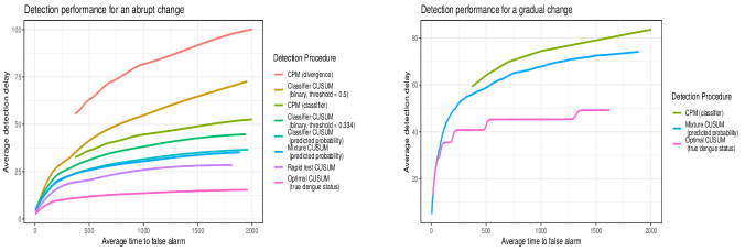
Figure 3: Left: Comparison of detection performance for CUSUM procedures using different detection procedures, for a change in dengue prevalence from $\pi_{\infty}=0.3$ to $\pi_{0}=0.68$. For ease, the method labels for the plot are displayed in descending order of detection delay. Right: Comparison of detection performance when $\pi_{0}$ changes gradually from $0.3$ to $0.68$.

5.5.2 Gradual change

Figure 3 shows the relationship between $\mathbb{E}_{\infty}[T]$ and $\mathbb{E}_{0}[T]$ for each method. Detection delays are longer for all methods under gradual change than abrupt change, because the magnitude of change is initially smaller. However, each method can raise an alarm reasonably quickly. This is valuable because real changes in prevalence are expected to be continuous, rather than an abrupt switch from one prevalence to another. While the classic CUSUM procedure, and the nonparametric methods discussed in this paper, are designed to detect an abrupt change, Figure 3 demonstrates that these methods are sensitive to other changes too.

6 Discussion

When a classifier is applied sequentially over time, it is important to detect any change in the distribution of classification data. First, distributional shifts can affect the validity of classifier predictions, and second, a change in distribution may suggest a problem like a disease outbreak. In this paper, we consider procedures for detecting label shift, which can occur when the prevalence of a disease changes over time, but the symptoms of the disease remain the same.

As we focus on detecting changes in classification data, it is natural to use the classifier predictions in our detection procedure. Here we propose a simple, nonparametric sequential changepoint detection method that uses the classifier predictions to approximate the true likelihood ratio (3). Our procedure requires no additional estimation or training, assuming only that a reasonable value of the post-change prevalence $\pi_{0}$ can be specified. Furthermore, when this post-change parameter is unknown, we combine our nonparametric procedure with Lai’s mixture CUSUM approach (Lai,, 1998), and mix over the unknown prevalence.

Performance of the detection procedure then depends directly on classifier performance. To demonstrate this, in Section 3 we introduce new convergence results for nonparametric sequential detection procedures with likelihood ratio estimates. Through simulations in Section 4, we illustrate that our proposed detection procedure outperforms other nonparametric methods when the label shift assumption holds, and still achieves comparable performance when the the label shift assumption is violated. The same holds true when these methods are applied to real dengue classification data in Section 5, in which we apply the classifier described in Tuan et al., (2015) to detect a simulated dengue outbreak. First, we see that improved classifier performance results in improved detection performance – if the gold standard dengue test is unavailable, only the NS1 rapid antigen test (which has better specificity than the classifier from Tuan et al., (2015)) outperforms our proposed procedure. Second, other nonparametric procedures respond more slowly to the outbreak, because they leverage less information about a change in prevalence.

While the label shift assumption might not hold exactly in real data, Rabanser et al., (2019) found that testing for label shift is still a useful way for finding more general changes in distribution. This is supported by our simulation results, in which our label shift detection procedure still performs well under mild violations of the label shift assumption.

Appendix A Supplementary Materials

A.1 Data and code

Full code for the data analysis and simulations presented in this paper is available at https://github.com/ciaran-evans/label-shift-detection. The data used in the dengue case study was made publicly available by Tuan et al., (2015), and a copy is provided in the repository with the code.

A.2 Proof of Theorem 1

Proof.

Following Tartakovsky et al., (2009), we can express the desired expectations as solutions to Fredholm integral equations of the second kind. In particular, let $v_{1}(x)=\mathbb{E}_{i}(T^{x}(A))$, and $v_{2}(x)=\mathbb{E}_{i}(\widetilde{T}^{x}(A)|\widehat{\lambda}_{m})$. Then,

$$v_{1}(x) =1+\int\limits_{0}^{A}v_{1}(y)k(x,y)dy$$ (13)

$$v_{2}(x) =1+\int\limits_{0}^{A}v_{2}(y)\widetilde{k}(x,y)dy,$$ (14)

where $k(x,y)=\frac{\partial}{\partial y}\mathbb{P}_{i}\left(\lambda(X)\leq\frac{y}{\Psi(x)}\right)$ (Tartakovsky et al.,, 2009), and $\widetilde{k}(x,y)=\frac{\partial}{\partial y}\mathbb{P}_{i}\left(\widehat{\lambda}_{m}(X)\leq\frac{y}{\Psi(x)}|\widehat{\lambda}_{m}\right)$. Using this representation, we show that $||v_{1}-v_{2}||_{\infty}$ is small.

First, let $K$ and $\widetilde{K}$ be the integral operators defined by the kernels $k(x,y)$ and $\widetilde{k}(x,y)$. Then under assumption (A3), we have $K,\widetilde{K}:C([0,A])\to C([0,A])$ are compact (Han and Atkinson,, 2009). Furthermore, $v_{1}=(I-K)\bm{1}$ and $v_{2}=(I-\widetilde{K})\bm{1}$, where $\bm{1}(x)\equiv 1$.

Next we show that $Kv=v$ and $\widetilde{K}v=v$ have only the trivial solution $v=0$. Considering $K,\widetilde{K}$ on $L^{2}(0,A)$, we have $K,\widetilde{K}:L^{2}(0,A)\to L^{2}(0,A)$ because $k,\widetilde{k}$ are Hilbert-Schmidt kernel functions under (A3). Then consider the adjoint operators $K^{*}$ and $\widetilde{K}^{*}$. Moustakides et al., (2011) demonstrate that the maximal eigenvalue of $K^{*}$ is strictly less than 1 when $\lambda(X)$ is continuous, and therefore the same holds for $K$. So, $Kv=v$ has only the trivial solution $v=0$, with the same result for $\widetilde{K}$.

Then by the Fredholm alternative theorem, $(I-K)^{-1},(I-\widetilde{K})^{-1}:C([0,A])\to C([0,A])$ are bijective and bounded (Han and Atkinson,, 2009). Furthermore,

$$||K-\widetilde{K}||_{\infty}\leq\sup\limits_{x\in[0,A]}\int\limits_{0}^{A}|k(x,y)-\widetilde{k}(x,y)|dy\leq\int\limits_{0}^{\infty}|f^{i}_{\lambda}(s)-f^{i}_{\widehat{\lambda}_{m}}(s)|ds=2TV(f^{i}_{\lambda},f^{i}_{\widehat{\lambda}_{m}}).$$ (15)

By (A5), $TV(f^{i}_{\lambda},f^{i}_{\widehat{\lambda}_{m}})\overset{p}{\to}0$, and so by Theorem 2.3.5 in Han and Atkinson, (2009), we have that

$$|\mathbb{E}_{i}(\widetilde{T}^{x}(A)|\widehat{\lambda}_{m})-\mathbb{E}_{i}(T^{x}(A))|\leq||v_{2}-v_{1}||_{\infty}\leq||\widetilde{K}^{-1}||_{\infty}||(K-\widetilde{K})v_{1}||_{\infty}\leq O_{P}(TV(f^{i}_{\lambda},f^{i}_{\widehat{\lambda}_{m}})).$$ (16)

Finally, we can improve the bound in the case when $f^{i}_{\lambda}$ is bounded. Note that

$$\begin{split}\left\lvert\int\limits_{0}^{A}(k(x,y)-\widetilde{k}(x,y))v_{1}(y)dy\right\rvert&\leq\left\lvert\int\limits_{0}^{\infty}f_{\Psi(x)\lambda}(y)\overline{v}_{1}(y)dy-\int\limits_{0}^{\infty}f_{\Psi(x)\widehat{\lambda}_{m}}(y)\overline{v}_{1}(y)dy\right\rvert\\ &\hskip 14.22636pt+v_{1}(A)\left\lvert\int\limits_{A}^{\infty}(f_{\Psi(x)\lambda}(y)-f_{\Psi(x)\widehat{\lambda}_{m}}(y))dy\right\rvert,\end{split}$$ (17)

where $\overline{v}_{1}(y)=v_{1}(y)$ for $y\leq A$, and $\overline{v}_{1}(y)=v_{1}(A)$ for $y\geq A$. If $f^{i}_{\lambda}$ is bounded, then $v_{1}$ is Lipschitz, and

$$\left\lvert\int\limits_{0}^{\infty}f_{\Psi(x)\lambda}(y)\overline{v}_{1}(y)dy-\int\limits_{0}^{\infty}f_{\Psi(x)\widehat{\lambda}_{m}}(y)\overline{v}_{1}(y)dy\right\rvert \leq C\sup\limits_{||h||_{L}\leq 1}\left\lvert\int\limits_{0}^{\infty}f_{\Psi(x)\lambda}(y)h(y)dy-\int\limits_{0}^{\infty}f_{\Psi(x)\widehat{\lambda}_{m}}(y)h(y)dy\right\rvert$$ (18)

$$\leq C\Psi(A)\mathbb{E}_{i}[|\widehat{\lambda}_{m}(X)-\lambda(X)|],$$ (19)

by Kantorovich-Rubinstein duality. Since $\left\lvert\int\limits_{A}^{\infty}(f_{\Psi(x)\lambda}(y)-f_{\Psi(x)\widehat{\lambda}_{m}}(y))dy\right\rvert\leq||F^{i}_{\lambda}-F^{i}_{\widehat{\lambda}_{m}}||_{\infty}$, this concludes the proof. ∎

A.3 Proof of Corollary 1

Proof.

The proof of Corollary 1 is similar to the proof of Theorem 1, but in a finite-dimensional space. Since $\pi_{0}$ and $\pi_{\infty}$ are known, and $\log(\pi_{0}/\pi_{\infty})$ and $\log((1-\pi_{0})/(1-\pi_{\infty}))$ are both rational, then $R_{t}^{x}$ and $\widetilde{R}_{t}^{x}$ are Markov chains on the same finite state space, where $x$ and the states are linear combinations of $\log(\pi_{0}/\pi_{\infty})$ and $\log((1-\pi_{0})/(1-\pi_{\infty}))$. Let $v_{1}$ denote the vector of expected stopping times when starting the optimal detection procedure in each state, and $v_{2}$ the corresponding vector for the estimated detection procedure. Then, $(I-K)v_{1}=\bm{1}$ and $(I-\widetilde{K})v_{2}=\bm{1}$, where $\bm{1}$ is the vector of all 1’s, and $K$ and $\widetilde{K}$ are transition probability matrices for the Markov chain.

In particular, all elements of $K$ are either 0, $\mathbb{P}(Y_{i}=0)$, or $\mathbb{P}(Y_{i}=1)$. The corresponding elements of $\widetilde{K}$ are

$$\widetilde{K}_{ij}=\begin{cases}0&K_{ij}=0\\ \mathbb{P}(\mathcal{A}(X)=0|\mathcal{A})&K_{ij}=\mathbb{P}(Y_{i}=0)\\ \mathbb{P}(\mathcal{A}(X)=1|\mathcal{A})&K_{ij}=\mathbb{P}(Y_{i}=1).\end{cases}$$ (20)

Therefore, $|\widetilde{K}_{ij}-K_{ij}|\leq O_{P}(\mathbb{P}_{i}(\mathcal{A}(X)=0|Y=1,\mathcal{A})+\mathbb{P}_{i}(\mathcal{A}(X)=1|Y=0,\mathcal{A}))$, and as in Theorem 1 the proof follows again by applying Theorem 2.3.5 from Han and Atkinson, (2009). ∎

A.4 Proof of Theorem 2

Proof.

For ease of notation, we drop the subscript $i\in\{0,\infty\}$ and the dependence on the classifier $\mathcal{A}$ from the expectations; our goal is to show $|\mathbb{E}(\widetilde{T}_{w}(A))-\mathbb{E}(T_{w}(A))|\overset{p}{\to}0$. Let $U_{t}(A)=\min\{T_{w}(A),t\}$ and $\widetilde{U}_{t}(A)=\min\{\widetilde{T}_{w}(A),t\}$. Then for any $t_{0}>0$,

$$\begin{split}|\mathbb{E}(\widetilde{T}_{w}(A))-\mathbb{E}(T_{w}(A))|&\leq|\mathbb{E}(\widetilde{T}_{w}(A))-\mathbb{E}(\widetilde{U}_{t_{0}}(A))|+|\mathbb{E}(\widetilde{U}_{t_{0}}(A))-\mathbb{E}(U_{t_{0}}(A))|+\\ &\hskip 14.22636pt|\mathbb{E}(U_{t_{0}}(A))-\mathbb{E}(T_{w}(A))|.\end{split}$$ (21)

For $\varepsilon>0$, let $\mathcal{C}_{t_{0},\varepsilon}=\left\{X_{1},...,X_{t_{0}}:\sup\limits_{t\leq t_{0}}|\widetilde{R}_{t,w}-R_{t,w}|<\varepsilon|\mathcal{A}\right\}$. Then

$$|\mathbb{E}(\widetilde{U}_{t_{0}}(A))-\mathbb{E}(U_{t_{0}}(A))|\leq|\mathbb{E}(\widetilde{U}_{t_{0}}(A))-\mathbb{E}(\widetilde{U}_{t_{0}}(A)|\mathcal{C}_{t_{0},\varepsilon})|+|\mathbb{E}(\widetilde{U}_{t_{0}}(A)|\mathcal{C}_{t_{0},\varepsilon})-\mathbb{E}(U_{t_{0}}(A))|,$$ (22)

and $|\mathbb{E}(\widetilde{U}_{t_{0}}(A))-\mathbb{E}(\widetilde{U}_{t_{0}}(A)|\mathcal{C}_{t_{0},\varepsilon})|\leq 2t_{0}(1-\mathbb{P}(\mathcal{C}_{t_{0},\varepsilon}))$. Also, if $X_{1},...,X_{t_{0}}\in\mathcal{C}_{t_{0},\varepsilon}$ then $U_{t_{0}}(A-\varepsilon)\leq\widetilde{U}_{t_{0}}(A)\leq U_{t_{0}}(A+\varepsilon)$, and so

$$\begin{split}|\mathbb{E}(\widetilde{U}_{t_{0}}(A)|\mathcal{C}_{t_{0},\varepsilon})-\mathbb{E}(U_{t_{0}}(A))|&\leq|\mathbb{E}(U_{t_{0}}(A+\varepsilon))-\mathbb{E}(T_{w}(A+\varepsilon))|+|\mathbb{E}(T_{w}(A+\varepsilon))-\mathbb{E}(T_{w}(A-\varepsilon))|+\\ &\hskip 14.22636pt|\mathbb{E}(T_{w}(A-\varepsilon))-\mathbb{E}(U_{t_{0}}(A-\varepsilon))|.\end{split}$$ (23)

Now let $\eta>0$. By continuity of $\mathbb{E}(T_{w}(A))$, there exists $\varepsilon>0$ such that $|\mathbb{E}(T_{w}(A+\varepsilon))-\mathbb{E}(T_{w}(A-\varepsilon))|<\eta/6$. Next, let $c_{1}>0$ and $0<\delta_{1}<\min\{\frac{a}{\pi_{\infty}},\frac{1-b}{1-\pi_{\infty}}\}$. For $\pi_{0}\in\Pi_{0}$, define $\lambda_{\pi_{0}}^{\min}$ by

$$\lambda_{\pi_{0}}^{\min}(x)=\begin{cases}\lambda_{\pi_{0}}(x)-\delta_{1}&x\in\mathcal{S}_{c_{1}}\\ \min\{\frac{a}{\pi_{\infty}},\frac{1-b}{1-\pi_{\infty}}\}&x\not\in\mathcal{S}_{c_{1}},\end{cases}$$ (24)

and define $T_{w}^{\min}$ by replacing $\lambda_{\pi_{0}}$ with $\lambda_{\pi_{0}}^{\min}$ in (6), and where we choose $\delta_{1}$ and $c_{1}$ sufficiently small that $\mathbb{E}(T_{w}^{\min})$ is finite. Therefore, if $\sup\limits_{\begin{subarray}{c}x\in\mathcal{S}_{c_{1}}\\ \pi_{0}\in\Pi_{0}\end{subarray}}|\widehat{\lambda}_{\pi_{0},\mathcal{A},m}(x)-\lambda_{\pi_{0}}(x)|<\delta_{1}$, then $|\mathbb{E}(\widetilde{T}_{w}(A))-\mathbb{E}(\widetilde{U}_{t_{0}}(A))|\leq|\mathbb{E}(T_{w}^{\min}(A))-\mathbb{E}(U_{t_{0}}^{\min}(A))|$.

Now choose $t_{0}$ sufficiently large that

$$\begin{split}|\mathbb{E}(T_{w}^{\min}(A))-\mathbb{E}(U_{t_{0}}^{\min}(A))|&<\eta/6\\ |\mathbb{E}(U_{t_{0}}(A+\varepsilon))-\mathbb{E}(T_{w}(A+\varepsilon))|&<\eta/6\\ |\mathbb{E}(U_{t_{0}}(A-\varepsilon))-\mathbb{E}(T_{w}(A-\varepsilon))|&<\eta/6\\ |\mathbb{E}(U_{t_{0}}(A))-\mathbb{E}(T_{w}(A))|&<\eta/6.\end{split}$$ (25)

Finally, we just have to control $2t_{0}(1-\mathbb{P}(\mathcal{C}_{t_{0},\varepsilon}))$. If $\sup\limits_{\begin{subarray}{c}x\in\mathcal{S}_{c}\\ \pi_{0}\in\Pi_{0}\end{subarray}}|\widehat{\lambda}_{\pi_{0},\mathcal{A},m}(x)-\lambda_{\pi_{0}}(x)|<\delta$ and $X_{1},...,X_{t_{0}}\in\mathcal{S}_{c}$, then

$$\begin{split}\sup\limits_{t\leq t_{0}}|\widetilde{R}_{t,w}-R_{t,w}|&=\sup\limits_{t\leq t_{0}}\left\lvert\max\limits_{t-m_{\alpha}\leq k\leq t}\int\limits_{\Pi_{0}}\prod\limits_{i=k}^{t}\widehat{\lambda}_{\pi_{0},\mathcal{A},m}(X_{i})w(\pi_{0})d\pi_{0}-\max\limits_{t-m_{\alpha}\leq k\leq t}\int\limits_{\Pi_{0}}\prod\limits_{i=k}^{t}\lambda_{\pi_{0}}(X_{i})w(\pi_{0})d\pi_{0}\right\rvert\\ \\ &\leq\sup\limits_{t\leq t_{0}}\max\limits_{t-m_{\alpha}\leq k\leq t}\left\lvert\int\limits_{\Pi_{0}}\prod\limits_{i=k}^{t}\widehat{\lambda}_{\pi_{0},\mathcal{A},m}(X_{i})w(\pi_{0})d\pi_{0}-\int\limits_{\Pi_{0}}\prod\limits_{i=k}^{t}\lambda_{\pi_{0}}(X_{i})w(\pi_{0})d\pi_{0}\right\rvert\\ &\leq\sup\limits_{t\leq t_{0}}\int\limits_{\Pi_{0}}\left(\max\limits_{t-m_{\alpha}\leq k\leq t}\left\lvert\prod\limits_{i=k}^{t}\widehat{\lambda}_{\pi_{0},\mathcal{A},m}(X_{i})-\prod\limits_{i=k}^{t}\lambda_{\pi_{0}}(X_{i})\right\rvert\right)w(\pi_{0})d\pi_{0}\\ &\leq\max\left\{(M+\delta)^{m_{\alpha}}-M^{m_{\alpha}},\ M^{m_{\alpha}}-(M-\delta)^{m_{\alpha}}\right\}.\end{split}$$ (26)

where $M=\max\left\{\frac{1}{\pi_{\infty}}\ ,\ \frac{1}{1-\pi_{\infty}}\right\}$. Choose $\delta_{2}<\delta_{1}$ such that the right hand side is at most $\varepsilon$, and $c_{2}<c_{1}$ such that $2t_{0}(1-\mathbb{P}(X_{i}\in\mathcal{S}_{c_{2}})^{t_{0}})<\eta/6$. Then, $\sup\limits_{\begin{subarray}{c}x\in\mathcal{S}_{c_{2}}\\ \pi_{0}\in\Pi_{0}\end{subarray}}|\widehat{\lambda}_{\pi_{0},\mathcal{A},m}(x)-\lambda_{\pi_{0}}(x)|<\delta_{2}$ implies that $|\mathbb{E}(\widetilde{T}_{w}(A))-\mathbb{E}(T_{w}(A))|<\eta$, and so

$$\mathbb{P}\left(|\mathbb{E}(\widetilde{T}_{w}(A))-\mathbb{E}(T_{w}(A))|<\eta\right)\geq\mathbb{P}\left(\sup\limits_{\begin{subarray}{c}x\in\mathcal{S}_{c_{2}}\\ \pi_{0}\in\Pi_{0}\end{subarray}}|\widehat{\lambda}_{\pi_{0},\mathcal{A},m}(x)-\lambda_{\pi_{0}}(x)|<\delta_{2}\right)\to 1.$$ (27)

As this works for all $\eta>0$, then we conclude that $|\mathbb{E}(\widetilde{T}_{w}(A))-\mathbb{E}(T_{w}(A))|\overset{p}{\to}0$ as desired. ∎

A.5 Details for Example 1

Under $\mathbb{P}_{\infty}$, $X\sim N(0,1)$ and under $\mathbb{P}_{0}$, $X\sim N(\mu,1)$. Therefore,

$$\lambda(x)=\frac{\exp\{-0.5(x-\mu)^{2}\}}{\exp\{-0.5x^{2}\}}=\exp\left\{\mu x-\frac{\mu^{2}}{2}\right\}.$$ (28)

Let $\widehat{\mu}$ be an estimate of $\mu$, then $\widehat{\lambda}(x)=\exp\left\{\widehat{\mu}x-\frac{\widehat{\mu}^{2}}{2}\right\}$.

Next, we need $f_{\lambda}^{i}$ and $f_{\widehat{\lambda}}^{i}$. Since $P(\widehat{\lambda}(X)\leq s)=P(X\leq\log(s)/\mu+\mu/2)$, then $f_{\lambda}^{i}(s)=f_{X}^{i}(\log(s)/\mu+\mu/2)/(\mu s)$. Likewise, $f_{\widehat{\lambda}}^{i}(s)=f_{X}^{i}(\log(s)/\widehat{\mu}+\widehat{\mu}/2)/(\widehat{\mu}s)$. Since the pre- and post-change distributions are normal, then

$$f_{\lambda}^{\infty}(s)\propto\frac{1}{\mu s}\exp\left\{-\frac{1}{2}\left(\frac{\log s}{\mu}+\frac{\mu}{2}\right)^{2}\right\}\hskip 14.22636ptf_{\widehat{\lambda}}^{\infty}(s)\propto\frac{1}{\widehat{\mu}s}\exp\left\{-\frac{1}{2}\left(\frac{\log s}{\widehat{\mu}}+\frac{\widehat{\mu}}{2}\right)^{2}\right\}$$ (29)

$$f_{\lambda}^{0}(s)\propto\frac{1}{\mu s}\exp\left\{-\frac{1}{2}\left(\frac{\log s}{\mu}-\frac{\mu}{2}\right)^{2}\right\}\hskip 14.22636ptf_{\widehat{\lambda}}^{\infty}(s)\propto\frac{1}{\widehat{\mu}s}\exp\left\{-\frac{1}{2}\left(\frac{\log s}{\widehat{\mu}}+\frac{\widehat{\mu}}{2}-\mu\right)^{2}\right\}.$$ (30)

Clearly, (A2) is satisfied. To show that (A3) is satisfied, we prove that $f_{\lambda}^{i}$ and $f_{\widehat{\lambda}}^{i}$ are Lipschitz. We have

$$\frac{d}{ds}f_{\lambda}^{\infty}(s) =\frac{1}{(\mu s)^{2}}\exp\left\{-\frac{1}{2}\left(\frac{\log s}{\mu}+\frac{\mu}{2}\right)^{2}\right\}\left(-\frac{\log s}{\mu}-\frac{3\mu}{2}\right)$$ (31)

$$\frac{d}{ds}f_{\lambda}^{0}(s) =\frac{1}{(\mu s)^{2}}\exp\left\{-\frac{1}{2}\left(\frac{\log s}{\mu}-\frac{\mu}{2}\right)^{2}\right\}\left(-\frac{\log s}{\mu}-\frac{\mu}{2}\right).$$ (32)

Since both derivatives are bounded, $f_{\lambda}^{\infty}$ and $f_{\lambda}^{0}$ are Lipschitz. Similarly, $f_{\widehat{\lambda}}^{\infty}$ and $f_{\widehat{\lambda}}^{0}$ are Lipschitz.

Finally, to show that (A5) is bounded, and provide the upper bound in Theorem 1, we need to show that $TV(f_{\widehat{\lambda}}^{i},f_{\lambda}^{i})\overset{p}{\to}0$. We have

$$|f_{\widehat{\lambda}}^{\infty}(s)-f_{\lambda}^{\infty}(s)| \leq\left|\frac{1}{\widehat{\mu}}-\frac{1}{\mu}\right|\left|\frac{1}{s}\exp\left\{-\frac{1}{2}\left(\frac{\log s}{\widehat{\mu}}+\frac{\widehat{\mu}}{2}\right)\right\}\right|$$ (33)

$$+\frac{1}{\mu}\left|\frac{1}{s}\exp\left\{-\frac{1}{2}\left(\frac{\log s}{\widehat{\mu}}+\frac{\widehat{\mu}}{2}\right)^{2}\right\}-\frac{1}{s}\exp\left\{-\frac{1}{2}\left(\frac{\log s}{\mu}+\frac{\mu}{2}\right)^{2}\right\}\right|.$$ (34)

First,

$$\int\limits_{0}^{\infty}\left|\frac{1}{\widehat{\mu}}-\frac{1}{\mu}\right|\left|\frac{1}{s}\exp\left\{-\frac{1}{2}\left(\frac{\log s}{\widehat{\mu}}+\frac{\widehat{\mu}}{2}\right)\right\}\right|ds=O_{P}\left(\left|\frac{1}{\widehat{\mu}}-\frac{1}{\mu}\right|\right)=O_{P}(|\widehat{\mu}-\mu|).$$ (35)

Next,

$$\begin{split}\left|\frac{1}{s}\exp\left\{-\frac{1}{2}\left(\frac{\log s}{\widehat{\mu}}+\frac{\widehat{\mu}}{2}\right)^{2}\right\}-\frac{1}{s}\exp\left\{-\frac{1}{2}\left(\frac{\log s}{\mu}+\frac{\mu}{2}\right)^{2}\right\}\right|&=|\widehat{\mu}-\mu|\left|\frac{1}{\mu^{3}s}e^{-0.125(\mu^{2}+2\log s)^{2}/\mu^{2}}(\log^{2}(s)-0.25\mu^{4})\right|\\ &+O_{P}(|\widehat{\mu}-\mu|^{2}),\end{split}$$ (36)

and

$$\int\limits_{0}^{\infty}|\widehat{\mu}-\mu|\left|\frac{1}{\mu^{3}s}e^{-0.125(\mu^{2}+2\log s)^{2}/\mu^{2}}(\log^{2}(s)-0.25\mu^{4})\right|ds=O_{P}(|\widehat{\mu}-\mu|).$$ (37)

Therefore,

$$TV(f_{\widehat{\lambda}}^{i},f_{\lambda}^{i})=\int\limits_{0}^{\infty}|f_{\widehat{\lambda}}^{\infty}(s)-f_{\lambda}^{\infty}(s)|ds\leq O_{P}(|\widehat{\mu}-\mu|).$$ (38)

A.6 Details for Example 2

Under both pre- and post-change distributions, $X|Y=y\sim N(\bm{\mu_{y}},\bm{\Sigma})$. Let $p(x)=\mathbb{P}_{\infty}(Y=1|X=x)$, and let $\mathcal{A}$ be the LDA classifier with predicted probabilities $\mathcal{A}(x)=\widehat{\mathbb{P}}_{\infty}(Y=1|X=x)$, given by (11). Then, $\lambda(X)$ and $\widehat{\lambda}(X)$ are linear transformations of $p(X)$ and $\mathcal{A}(X)$ respectively, by (2) and (3). Therefore, to check the assumptions it is sufficient to consider $f_{p|Y=y}$ and $f_{\mathcal{A}|Y=y}$, the conditional densities of $p(X)|Y=y$ and $\mathcal{A}(X)|Y=y$.

First, we have

$$\begin{split}f_{p|Y=y}(s)&=\frac{1}{s-s^{2}}\phi\left(\frac{\log\left(\frac{s(1-\pi_{\infty})}{(1-s)\pi_{\infty}}\right)+\frac{1}{2}\left(\bm{\mu_{1}}^{T}\bm{\Sigma}^{-1}\bm{\mu_{1}}-\bm{\mu_{0}}^{T}\bm{\Sigma}^{-1}\bm{\mu_{0}}\right)-\bm{\mu_{y}}^{T}\bm{\Sigma}^{-1}(\bm{\mu_{1}}-\bm{\mu_{0}})}{\sqrt{(\bm{\mu_{1}}-\bm{\mu_{0}})^{T}\bm{\Sigma}^{-1}(\bm{\mu_{1}}-\bm{\mu_{0}})}}\right)\\ f_{\mathcal{A}|Y=y}(s)&=\frac{1}{s-s^{2}}\phi\left(\frac{\log\left(\frac{s(1-\pi_{\infty})}{(1-s)\pi_{\infty}}\right)+\frac{1}{2}\left(\widehat{\bm{\mu_{1}}}^{T}\widehat{\bm{\Sigma}}^{-1}\widehat{\bm{\mu_{1}}}-\widehat{\bm{\mu_{0}}}^{T}\widehat{\bm{\Sigma}}^{-1}\widehat{\bm{\mu_{0}}}\right)-\bm{\mu_{y}}^{T}\widehat{\bm{\Sigma}}^{-1}(\widehat{\bm{\mu_{1}}}-\widehat{\bm{\mu_{0}}})}{\sqrt{(\widehat{\bm{\mu_{1}}}-\widehat{\bm{\mu_{0}}})^{T}\widehat{\bm{\Sigma}}^{-1}\bm{\Sigma}\widehat{\bm{\Sigma}}^{-1}(\widehat{\bm{\mu_{1}}}-\widehat{\bm{\mu_{0}}})}}\right),\end{split}$$ (39)

where $\phi$ is the standard normal density. For simplicity, we write this as

$$\begin{split}f_{p|Y=y}(s)&=\frac{1}{s-s^{2}}\phi\left(\frac{\log\left(\frac{s(1-\pi_{\infty})}{(1-s)\pi_{\infty}}\right)+a}{b}\right)\\ f_{\mathcal{A}|Y=y}(s)&=\frac{1}{s-s^{2}}\phi\left(\frac{\log\left(\frac{s(1-\pi_{\infty})}{(1-s)\pi_{\infty}}\right)+\widehat{a}}{\widehat{b}}\right).\end{split}$$ (40)

Now, we show that these densities are Lipschitz. For $p(X)|Y=y$, we have

$$\frac{d}{ds}f_{p|Y=y}=\frac{\left(-a+b^{2}(2s-1)-\log\left(\frac{s(1-\pi_{\infty})}{(1-s)\pi_{\infty}}\right)\right)}{b^{2}(1-s^{2})s^{2}},$$ (41)

which is bounded. Similarly, $\frac{d}{ds}f_{\mathcal{A}|Y=y}$ is bounded. Therefore, $f_{p|Y=y}$ and $f_{\mathcal{A}|Y=y}$ are Lipschitz, so $f_{\lambda}^{i}$ and $f_{\widehat{\lambda}}^{i}$ are all Lipschitz, which satisfies (A3).

Next, we want to show convergence in total variation distance. Note that $|f_{\lambda}^{i}-f_{\widehat{\lambda}}^{i}|=O_{P}(|f_{p|Y=1}-f_{\mathcal{A}|Y=1}|)+O_{P}(|f_{p|Y=0}-f_{\mathcal{A}|Y=0}|)$, so it suffices to show that $TV(f_{p|Y=y},f_{\mathcal{A}|Y=y})$ converges. Using $a,\widehat{a},b,\widehat{b}$ from above, we get

$$TV(f_{p|Y=y},f_{\mathcal{A}|Y=y})=\int|f_{\mathcal{A}|Y=y}(s)-f_{p|Y=y}(s)|ds=O_{P}(|\widehat{a}-a|)+O_{P}(|\widehat{b}-b|).$$ (42)

The right hand side converges by strong consistency of $\widehat{\bm{\mu_{y}}}$, $y\in\{0,1\}$, and $\widehat{\bm{\Sigma}}^{-1}$, satisfying (A5).

References

- Ackerman et al., (2020) Ackerman, S., Dube, P., and Farchi, E. (2020). Sequential drift detection in deep learning classifiers. arXiv preprint arXiv:2007.16109.
- Azizzadenesheli et al., (2019) Azizzadenesheli, K., Liu, A., Yang, F., and Anandkumar, A. (2019). Regularized learning for domain adaptation under label shifts. arXiv preprint arXiv:1903.09734.
- Baron, (2000) Baron, M. I. (2000). Nonparametric adaptive change point estimation and on line detection. Sequential Analysis, 19(1-2):1–23.
- Bell et al., (1994) Bell, C., Gordon, L., and Pollak, M. (1994). An efficient nonparametric detection scheme and its application to surveillance of a bernoulli process with unknown baseline. Lecture Notes-Monograph Series, pages 7–27.
- Bickel et al., (2009) Bickel, S., Brückner, M., and Scheffer, T. (2009). Discriminative learning under covariate shift. Journal of Machine Learning Research, 10(9).
- Brodsky and Darkhovsky, (1993) Brodsky, E. and Darkhovsky, B. S. (1993). Nonparametric methods in change point problems, volume 243. Springer Science & Business Media.
- Brodsky and Darkhovsky, (2000) Brodsky, E. and Darkhovsky, B. S. (2000). Non-parametric statistical diagnosis: problems and methods, volume 509. Springer Science & Business Media.
- Chen, (2019) Chen, H. (2019). Sequential change-point detection based on nearest neighbors. The Annals of Statistics, 47(3):1381–1407.
- Chen and Chu, (2019) Chen, H. and Chu, L. (2019). gStream: Graph-Based Sequential Change-Point Detection for Streaming Data. R package version 0.2.0.
- Cheng et al., (2020) Cheng, J., Bambrick, H., Yakob, L., Devine, G., Frentiu, F. D., Thai, P. Q., Xu, Z., Hu, W., et al. (2020). Heatwaves and dengue outbreaks in hanoi, vietnam: New evidence on early warning. PLoS neglected tropical diseases, 14(1):e0007997.
- Chu and Chen, (2018) Chu, L. and Chen, H. (2018). Sequential change-point detection for high-dimensional and non-euclidean data. arXiv preprint arXiv:1810.05973.
- Cipolli and Hanson, (2017) Cipolli, W. and Hanson, T. (2017). Computationally tractable approximate and smoothed polya trees. Statistics and Computing, 27(1):39–51.
- Cipolli and Hanson, (2019) Cipolli, W. and Hanson, T. (2019). Supervised learning via smoothed polya trees. Advances in Data Analysis and Classification, 13(4):877–904.
- Cuong et al., (2011) Cuong, H. Q., Hien, N. T., Duong, T. N., Phong, T. V., Cam, N. N., Farrar, J., Nam, V. S., Thai, K. T., and Horby, P. (2011). Quantifying the emergence of dengue in hanoi, vietnam: 1998–2009. PLoS Negl Trop Dis, 5(9):e1322.
- Garg et al., (2011) Garg, A., Garg, J., Rao, Y., Upadhyay, G., and Sakhuja, S. (2011). Prevalence of dengue among clinically suspected febrile episodes at a teaching hospital in north india. Journal of Infectious Diseases and Immunity, 3(5):85–89.
- Giné and Guillou, (2002) Giné, E. and Guillou, A. (2002). Rates of strong uniform consistency for multivariate kernel density estimators. In Annales de l’Institut Henri Poincare (B) Probability and Statistics, volume 38, pages 907–921. Elsevier.
- Gordon and Pollak, (1994) Gordon, L. and Pollak, M. (1994). An efficient sequential nonparametric scheme for detecting a change of distribution. The Annals of Statistics, pages 763–804.
- Gordon and Pollak, (1995) Gordon, L. and Pollak, M. (1995). A robust surveillance scheme for stochastically ordered alternatives. The Annals of Statistics, pages 1350–1375.
- Gretton et al., (2009) Gretton, A., Smola, A., Huang, J., Schmittfull, M., Borgwardt, K., and Schölkopf, B. (2009). Covariate shift by kernel mean matching. Dataset shift in machine learning, 3(4):5.
- Han and Atkinson, (2009) Han, W. and Atkinson, K. E. (2009). Theoretical Numerical Analysis: A Functional Analysis Framework. Springer.
- Hsu et al., (2017) Hsu, J. C., Hsieh, C.-L., and Lu, C. Y. (2017). Trend and geographic analysis of the prevalence of dengue in taiwan, 2010–2015. International Journal of Infectious Diseases, 54:43–49.
- Kanamori et al., (2009) Kanamori, T., Hido, S., and Sugiyama, M. (2009). A least-squares approach to direct importance estimation. Journal of Machine Learning Research, 10(Jul):1391–1445.
- Kanamori et al., (2012) Kanamori, T., Suzuki, T., and Sugiyama, M. (2012). Statistical analysis of kernel-based least-squares density-ratio estimation. Machine Learning, 86(3):335–367.
- Kawahara and Sugiyama, (2009) Kawahara, Y. and Sugiyama, M. (2009). Change-point detection in time-series data by direct density-ratio estimation. In Proceedings of the 2009 SIAM International Conference on Data Mining, pages 389–400. SIAM.
- Lai, (1998) Lai, T. L. (1998). Information bounds and quick detection of parameter changes in stochastic systems. IEEE Transactions on Information Theory, 44(7):2917–2929.
- Lipton et al., (2018) Lipton, Z. C., Wang, Y.-X., and Smola, A. (2018). Detecting and correcting for label shift with black box predictors. arXiv preprint arXiv:1802.03916.
- Liu et al., (2013) Liu, S., Yamada, M., Collier, N., and Sugiyama, M. (2013). Change-point detection in time-series data by relative density-ratio estimation. Neural Networks, 43:72–83.
- Lorden, (1971) Lorden, G. (1971). Procedures for reacting to a change in distribution. The Annals of Mathematical Statistics, 42(6):1897–1908.
- Madrid Padilla et al., (2019) Madrid Padilla, O. H., Athey, A., Reinhart, A., and Scott, J. G. (2019). Sequential nonparametric tests for a change in distribution: an application to detecting radiological anomalies. Journal of the American Statistical Association, 114(526):514–528.
- Makiyama, (2019) Makiyama, K. (2019). densratio: Density Ratio Estimation. R package version 0.2.1.
- McDonald, (1990) McDonald, D. (1990). A CUSUM procedure based on sequential ranks. Naval Research Logistics, 37(5):627–646.
- Moustakides, (1986) Moustakides, G. V. (1986). Optimal stopping times for detecting changes in distributions. The Annals of Statistics, 14(4):1379–1387.
- Moustakides et al., (2011) Moustakides, G. V., Polunchenko, A. S., and Tartakovsky, A. G. (2011). A numerical approach to performance analysis of quickest change-point detection procedures. Statistica Sinica, pages 571–596.
- Nguyen et al., (2010) Nguyen, X., Wainwright, M. J., and Jordan, M. I. (2010). Estimating divergence functionals and the likelihood ratio by convex risk minimization. IEEE Transactions on Information Theory, 56(11):5847–5861.
- Page, (1954) Page, E. S. (1954). Continuous inspection schemes. Biometrika, 41(1/2):100–115.
- Polunchenko and Tartakovsky, (2012) Polunchenko, A. S. and Tartakovsky, A. G. (2012). State-of-the-art in sequential change-point detection. Methodology and computing in applied probability, 14(3):649–684.
- Rabanser et al., (2019) Rabanser, S., Günnemann, S., and Lipton, Z. (2019). Failing loudly: An empirical study of methods for detecting dataset shift. Advances in Neural Information Processing Systems 32.
- Reynolds Jr and Stoumbos, (1999) Reynolds Jr, M. R. and Stoumbos, Z. G. (1999). A cusum chart for monitoring a proportion when inspecting continuously. Journal of quality technology, 31(1):87–108.
- Ross, (2015) Ross, G. J. (2015). Parametric and nonparametric sequential change detection in R: The cpm package. Journal of Statistical Software, 66(3):1–20.
- Ross and Adams, (2012) Ross, G. J. and Adams, N. M. (2012). Two nonparametric control charts for detecting arbitrary distribution changes. Journal of Quality Technology, 44(2):102–116.
- Ross et al., (2011) Ross, G. J., Tasoulis, D. K., and Adams, N. M. (2011). Nonparametric monitoring of data streams for changes in location and scale. Technometrics, 53(4):379–389.
- Saerens et al., (2002) Saerens, M., Latinne, P., and Decaestecker, C. (2002). Adjusting the outputs of a classifier to new a priori probabilities: a simple procedure. Neural computation, 14(1):21–41.
- Siegmund and Venkatraman, (1995) Siegmund, D. and Venkatraman, E. (1995). Using the generalized likelihood ratio statistic for sequential detection of a change-point. The Annals of Statistics, pages 255–271.
- Stone, (1982) Stone, C. J. (1982). Optimal global rates of convergence for nonparametric regression. The annals of statistics, pages 1040–1053.
- Storkey, (2009) Storkey, A. (2009). When training and test sets are different: characterizing learning transfer. Dataset shift in machine learning, pages 3–28.
- Sugiyama et al., (2008) Sugiyama, M., Suzuki, T., Nakajima, S., Kashima, H., von Bünau, P., and Kawanabe, M. (2008). Direct importance estimation for covariate shift adaptation. Annals of the Institute of Statistical Mathematics, 60(4):699–746.
- Tartakovsky et al., (2014) Tartakovsky, A., Nikiforov, I., and Basseville, M. (2014). Sequential analysis: Hypothesis testing and changepoint detection. Chapman and Hall/CRC.
- (48) Tartakovsky, A. G., Pollak, M., and Polunchenko, A. S. (2012a). Third-order asymptotic optimality of the generalized shiryaev–roberts changepoint detection procedures. Theory of Probability & Its Applications, 56(3):457–484.
- Tartakovsky et al., (2009) Tartakovsky, A. G., Polunchenko, A. S., and Moustakides, G. V. (2009). Design and comparison of shiryaev–roberts-and cusum-type change-point detection procedures. In Proceedings of the 2nd International Workshop in Sequential Methodologies.
- (50) Tartakovsky, A. G., Polunchenko, A. S., and Sokolov, G. (2012b). Efficient computer network anomaly detection by changepoint detection methods. IEEE Journal of Selected Topics in Signal Processing, 7(1):4–11.
- (51) Tartakovsky, A. G., Rozovskii, B. L., Blažek, R. B., and Kim, H. (2006a). Detection of intrusions in information systems by sequential change-point methods. Statistical methodology, 3(3):252–293.
- (52) Tartakovsky, A. G., Rozovskii, B. L., Blazek, R. B., and Kim, H. (2006b). A novel approach to detection of intrusions in computer networks via adaptive sequential and batch-sequential change-point detection methods. IEEE transactions on signal processing, 54(9):3372–3382.
- Tuan et al., (2015) Tuan, N. M., Nhan, H. T., Chau, N. V. V., Hung, N. T., Tuan, H. M., Van Tram, T., Le Da Ha, N., Loi, P., Quang, H. K., Kien, D. T. H., et al. (2015). Sensitivity and specificity of a novel classifier for the early diagnosis of dengue. PLoS Negl Trop Dis, 9(4):e0003638.
- Unnikrishnan et al., (2011) Unnikrishnan, J., Veeravalli, V. V., and Meyn, S. P. (2011). Minimax robust quickest change detection. IEEE Transactions on Information Theory, 57(3):1604–1614.
- WHO, (2020) WHO (2020). Dengue and severe dengue.
- Wiwanitkit, (2006) Wiwanitkit, V. (2006). An observation on correlation between rainfall and the prevalence of clinical cases of dengue in thailand. Journal of vector borne diseases, 43(2):73.
- Yu and Szepesvári, (2012) Yu, Y. and Szepesvári, C. (2012). Analysis of kernel mean matching under covariate shift. arXiv preprint arXiv:1206.4650.