The spatially resolved broad line region of IRAS 09149$-$6206

We present new near-infrared VLTI/GRAVITY interferometric spectra that spatially resolve the broad Br$\gamma$ emission line in the nucleus of the active galaxy IRAS 09149$-$6206. We use these data to measure the size of the broad line region (BLR) and estimate the mass of the central black hole. Using an improved phase calibration method that reduces the differential phase uncertainty to 0.05^∘ per baseline across the spectrum, we detect a differential phase signal that reaches a maximum of $\sim 0.5{\mbox{${}^{\circ}$}}$ between the line and continuum. This represents an offset of $\sim 120\,\mu$as (0.14 pc) between the BLR and the centroid of the hot dust distribution traced by the 2.3 $\mu$m continuum. The offset is well within the dust sublimation region, which matches the measured $\sim 0.6$ mas (0.7 pc) diameter of the continuum. A clear velocity gradient, almost perpendicular to the offset, is traced by the reconstructed photocentres of the spectral channels of the Br$\gamma$ line. We infer the radius of the BLR to be $\sim 65\,\mu$as (0.075 pc), which is consistent with the radius–luminosity relation of nearby active galactic nuclei derived based on the time lag of the H$\beta$ line from reverberation mapping campaigns. Our dynamical modelling indicates the black hole mass is $\sim 1\times 10^{8}\,M_{\odot}$, which is a little below, but consistent with, the standard $M_{\rm BH}$–$\sigma_{*}$ relation.

1 Introduction

Massive black holes in the centres of galaxies are a key component of galaxy evolution, because of the role that accreting black holes have in the feedback that regulates star formation and galaxy growth (Booth & Schaye, 2009; Fabian, 2012; Somerville & Davé, 2015; Dubois et al., 2016). Knowing their masses is central to our understanding of this co-evolution (Hopkins et al., 2008; Somerville et al., 2008; Kormendy & Ho, 2013; Heckman & Best, 2014), but measuring their masses robustly is challenging because it requires resolving spatial scales where the black hole dominates the gravitational potential (Ferrarese & Ford, 2005). For inactive galaxies, it can be done using spatially resolved stellar (e.g. Thomas et al., 2004; Onken et al., 2014; Saglia et al., 2016) or gas kinematics (Hicks & Malkan, 2008; Davis, 2014; Onishi et al., 2017; Boizelle et al., 2019). These methods can be difficult to apply to active galaxies displaying broad emission lines because the active galactic nucleus (AGN) itself is so bright, although it has been possible for a few objects (Davies et al., 2006). Instead, the most precise method for measuring black hole masses in AGNs is through megamaser kinematics using VLBI (Greene et al., 2010; Kuo et al., 2011). However, this requires the megamasers to be orbiting in a Keplerian disk restricted to near-edge-on view, which is very rare (Zhu et al., 2011; van den Bosch et al., 2016). Reverberation mapping (RM) exploits the variability of the black hole accretion to shed light on the size of the broad line region (BLR) and hence leads to a measurement of the black hole mass (Blandford & McKee, 1982; Peterson, 1993; Peterson et al., 2004). Despite potential biases (Shankar et al., 2019) and caveats in terms of the virial factor $f$ that reflects the unknown geometry and kinematics of the BLR (Onken et al., 2004; Woo et al., 2010; Ho & Kim, 2014), it has been used successfully for many years.

Spatially resolving the very small size of the BLR, $10^{3}-10^{5}$ gravitational radii (Netzer & Laor, 1993; Peterson, 1993; Netzer, 2015), has been a long-standing goal of spectroastrometry (Petrov et al., 2001; Marconi et al., 2003), that has recently become possible with long baseline near-infrared interferometry. GRAVITY, a second-generation VLTI instrument, has greatly improved both the sensitivity of earlier efforts, as well as combining all four of the 8-m Unit Telescope (UT) beams to yield six simultaneous baselines (Gravity Collaboration et al., 2017). In Gravity Collaboration et al. (2018, hereafter, GC18) we reported the first robust measurements of BLR size and kinematics for 3C 273 by combining differential phase spectra with the Pa$\alpha$ emission line profile to model the BLR as a thick rotating disk under the gravitational influence of a black hole of $\sim 3\times 10^{8}\,\rm{M}_{\sun}$. This value is fully consistent with the result of a subsequent study using 10-year RM data (Zhang et al., 2019). We have now embarked on a programme to make independent estimates of the black hole masses in a sample of AGN. The aim is not just to verify the masses derived through reverberation mapping, but to understand better the structure of the BLR, which has implications for inflow (accretion) and outflow processes on small scales.

The classical picture of the BLR is a virialized distribution of clouds, with good evidence that many are rotating systems. This comes from a variety of observations including variations in the polarisation properties across the broad line profile (Smith et al., 2004, 2005). In addition, a significant minority, $\sim 3\%$, of BLRs in both radio quiet and radio loud AGN show broad double-peaked profiles that are well fitted by disk emission (Eracleous & Halpern 1994, 2003; Strateva et al. 2003; Storchi-Bergmann et al. 2017). That rather few objects show such characteristics may be explained by the apparent relation between line width and shape, measured as FWHM/$\sigma$, reported by Kollatschny & Zetzl (2011). This suggests that rapidly rotating BLRs are flattened systems, while slower rotating BLRs have a more spherical structure due to turbulence. The turbulent velocities of 300–700 km s^-1 for H$\beta$ and 2000–4000 km s^-1 for C iv may be indicative of outflowing gas. Disk winds are theoretically appealing and apply in many different situations including AGN (Emmering et al., 1992; Murray et al., 1995; Dehghanian et al., 2020); and an outflow at a characteristic elevation of 30^∘ above the mid-plane is the basis of the concept proposed by Elvis (2000), a geometry that can explain a variety of observations including the broad absorption and broad emission lines. Rotating disk winds have been developed on a more physical basis by Everett (2005) and Keating et al. (2012); and PG 1700$+$518 is one example of a rotating outflow that has been observed (Young et al., 2007). It therefore seems likely that the dynamics of the BLR may be a combination of rotation and outflow in a way that depends on the properties of individual objects.

Recently, thanks to high signal-to-noise ratio (SNR) spectra, the non-parametric velocity-resolved RM analyses of tens of bright AGNs have begun to reveal this structure, through qualitative evidence for both inflow and outflow in addition to virial motion (e.g. Denney et al., 2009; Bentz et al., 2010; Peterson, 2014; Du et al., 2016a; De Rosa et al., 2018; Du et al., 2018a; Horne et al., 2020). Furthermore, temporal variation of the BLR geometry and dynamics has been reported for some AGNs (Pei et al., 2017; Pancoast et al., 2018; Xiao et al., 2018), implying that the virial factor of the same source may evolve with time.

Parametric models of the BLR geometry and dynamics have been successfully applied to less than two dozen AGNs that have both high SNR spectra and high cadence monitoring (Pancoast et al., 2014b; Grier et al., 2017a; Williams et al., 2018; Li & Wang, 2018). These enable one to fit for radial (inflow or outflow) motion of the clouds in addition to rotation, and hence also to derive the virial factors for individual objects. While the number of objects is too small for robust statistics, more than half of the BLRs are dominated by radial motion, with inflow and outflow being equally common. Remarkably, the black hole masses inferred from such dynamical modelling are usually consistent with those measured with the classical RM method, even when the BLR is dominated by outflow (Williams et al., 2018). However, there are degeneracies in the models (Grier et al., 2017a); and the impact of systematic uncertainties, such as the assumption that the ionisation source is point-like and that the BLR structure does not change significantly during the monitoring campaign, are challenging to assess (Pancoast et al., 2014a; Grier et al., 2017a). In particular, assumptions about the geometry of different BLR components may significantly bias the inferred physical interpretation (Mangham et al., 2019). As such, an independent method to constrain the BLR structure is much needed.

This role is fulfilled by optical/near-infrared long baseline interferometry combined with spectroastrometry. In this paper we present an analysis of new GRAVITY observations for IRAS 09149$-$6206 ($\alpha=09$:16:09.39, $\delta=-62$:19:29.9). Perez et al. (1989) serendipitously discovered IRAS 09149$-$6206 as an AGN in the IRAS Point Source Catalogue during a search for planetary nebulae after optical spectra showed characteristic broad Balmer lines. IRAS 09149$-$6206 is at a redshift of 0.0573 (Perez et al., 1989), which means that the broad Br$\gamma$ line can still be observed in the $K$-band and thus GRAVITY. Unfortunately, very little archival data exist for IRAS 09149$-$6206. It is detected in early radio continuum surveys, but not resolved (Murphy et al., 2007; Panessa et al., 2015). Existing optical/NIR images (e.g., Veron-Cetty & Woltjer 1990; Márquez et al. 1999) cannot constrain the morphological type of the host galaxy, and mid-infrared interferometric observations only barely resolve it (Kishimoto et al., 2011; Burtscher et al., 2013; López-Gonzaga et al., 2016). Section 2 describes the observations and data reduction including changes which significantly improve the precision of our differential phase spectra. In Section 3, we show that the model-independent photocentre positions reveal the detection of a spatial offset between the hot dust continuum and Br$\gamma$, and a velocity gradient across the emission line. Building on this, in Section 4 we adopt a kinematic cloud model to fit the phase data in order to constrain the BLR size and kinematics. In Section 5, we discuss the implications of our measured $M_{\rm BH}$ and place IRAS 09149$-$6206 on the BLR radius–luminosity relation. The possible interpretations of the offset between the BLR and the continuum is discussed in Section 6.

This work adopts the following parameters for a $\Lambda$CDM cosmology: $\Omega_{m}=0.308$, $\Omega_{\Lambda}=0.692$, and $H_{0}=67.8$ km s^-1 Mpc^-1 (Planck Collaboration et al., 2016). Using this cosmology, 1 pc subtends 0.87 mas on sky and 1 $\mu$as corresponds to 1.37 light day at the redshift of IRAS 09149$-$6206.

2 Observations and Data Reduction

Date	On-source	Seeing	Coherence
	time (min)	(″)	time (ms)
2018 Nov 20∗	55	0.65 $-$ 0.97	3.3$-$	4.2
2019 Feb 16†	75	0.53 $-$ 0.95	6.0$-$	9.1
2019 Nov 07∗	85	0.36 $-$ 0.71	6.5$-$	10.7
2019 Nov 09∗	30	0.42 $-$ 0.58	2.4$-$	4.2
2019 Dec 09∗	45	0.50 $-$ 0.71	1.8$-$	3.9
2020 Feb 09	55	0.47 $-$ 0.69	13.2$-$	15.4
2020 Feb 10†	75	0.51 $-$ 0.99	7.7$-$	13.2
2020 Mar 08†	45	0.49 $-$ 0.80	7.1$-$	9.9

Table 1: Exposure time and weather conditions for the observations. The reported data only include exposures for which we were able to track the fringe for $>80\%$ of the exposure time. The seeing and coherence time are based on measurements from the Differential Image Motion Monitor and Multi-aperture Scintillation Sensor on Paranal.
^∗ K stars are observed as calibrators.
^† B stars are observed as calibrators.

We observed IRAS 09149$-$6206 with GRAVITY (Gravity Collaboration et al., 2017) using all four UTs, on eight occasions between November 2018 and March 2020, primarily as part of a Large Programme to spatially resolve the BLR and measure black hole masses in a sample of AGN. Targets were selected as the brightest type 1 AGNs visible from the VLTI and above the GRAVITY sensitivity limit ($K<11$). IRAS 09149$-$6206, in particular, has more than 70% of its total $K$ band flux originating in the nucleus and is also bright and compact in the optical ($R\approx 11.5$). These properties make it an ideal GRAVITY target for observations where the source is phase referenced to itself as well as used for adaptive optics. We adopted the single-field on-axis mode for all of the observations with combined polarisation. The scientific spectra (1.95–2.45 $\mu$m) were taken in medium-resolution mode ($\lambda/\Delta\lambda\approx 500$), with 90 independent spectral elements, extracted and resampled into 210 channels.

All observations followed a similar sequence. After the telescope had pointed to the target and the adaptive optics (MACAO; Arsenault et al. 2003) had closed the loop, the telescope beams were coarsely aligned on the VLTI laboratory camera IRIS (Gitton et al., 2004). The light was then fed to GRAVITY and the internal beam tracking of GRAVITY aligned the fringe-tracking (FT) and science channel (SC) fibres on the target. After the fringe tracker had searched for and found the fringe, the scientific exposures were started. Each set of scientific exposures consisted of ten frames of 30-s integration (NDIT=10 and DIT=30 s). Fringe tracking is difficult for faint targets and leads to large phase noise ($\gtrsim 0.5{\mbox{${}^{\circ}$}}$). We therefore integrated deeply on-source, with only occasional sky exposures. In order to account for the observatory transfer function (e.g. coherence loss due to vibrations, uncorrected atmosphere, birefringence, etc.), we observed a calibrator star close to the science target. The calibrator data are used to calibrate the complex visibility and closure phase of the FT data, as well as the flux spectrum of the AGN. A calibrator was observed for all runs except 2020 Feb 09. The date, exposure time, and weather conditions for all observations are summarised in Table 1.

GRAVITY measures the complex visibilities of six baselines (telescope pairs). The visibility amplitudes measure the angular extent of a structure, whereas the phases provide its position and spatial distribution on the sky (e.g., Buscher & Longair 2015). The GRAVITY synthesis beam (about 3 mas) is usually much larger than the BLR of an AGN at cosmological distance and can only marginally resolve the continuum emission from the hot dust (Gravity Collaboration et al., 2018, 2020a). Therefore, the differential phase and differential visibility amplitude are the most important interferometric observables for the BLR. Spectro-astrometry (Bailey, 1998) enables us to spatially resolve the BLR, using the continuum as a reference. The differential phase measures the shift in the photocentre on sky at different wavelength channels of the broad line emission with respect to the continuum (see Appendix B). The differential visibility amplitude measures the relative size difference between the broad line emission and the continuum emission (see Section 4.4).

2.1 Pipeline data reduction

We used the latest version of the GRAVITY pipeline to reduce the data (Gravity Collaboration et al., 2017; Lapeyrere et al., 2014). This includes the recent improvements to lower the imprint of the internal source of the calibration unit (Blind et al., 2014), and a better filtering of hot pixels due to cosmic rays. For the FT continuum visibility data, we used the default pipeline settings. However, the low SNR of the FT data and loss of coherence during scientific exposures often caused the pipeline to flag most of the DITs in one scientific exposure. In analysing these data, we found a substantial improvement in residual phase noise (rms scatter) by retaining all data independent of FT SNR or the estimated visibility loss (GC18; Gravity Collaboration et al. 2020a, hereafter GC20a).

The pipeline reduces the data using a pixel-to-visibility matrix (Lapeyrere et al., 2014; Lacour et al., 2019). This matrix, encoding the relative throughput, coherence, phase shift, and cross-talk for each pixel, was measured during the day with the GRAVITY calibration unit after every night that GRAVITY observations were performed. Applying the matrix to the detector frames yields the instrument-calibrated complex visibilities. The pipeline then fits the phase of the science channel in each frame with a 3rd-order polynomial to derive the phase reference, which is then subtracted from the phase. This yields the self-referenced complex visibility for every frame. Before averaging the complex visibilities of an individual exposure, we applied the algorithm developed for VLTI/AMBER (Millour et al., 2008) to calculate and remove the average phase using all of the other wavelength channels for each channel. This method produces consistent results and improves our phase errors, typically by about 10%–20%. Initial uncertainties for the combined visibilities are estimated by bootstrapping the different frames in the pipeline. However, this underestimates the uncertainty, so we adopt a different method to estimate the phase uncertainty after the pipeline data reduction.

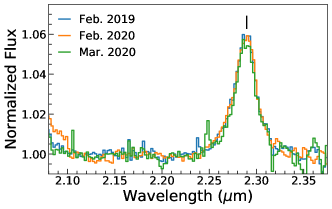
Figure 1: AGN flux spectra of IRAS 09149$-$6206 normalised to the continuum. The black vertical bar at 2.2896 $\mu$m marks the wavelength of Br$\gamma$ given a redshift $z=0.0573$ (Perez et al., 1989). We discard the wavelength ranges ($\lesssim 2.10\,{\mbox{$\mu$m}}$ and $\gtrsim 2.35\,{\mbox{$\mu$m}}$) that are significantly affected by the atmospheric absorption.

2.2 Normalised profile of the broad Br$\gamma$ line

The emission line profile, normalised to the continuum, is necessary to derive the velocity gradient and model the dynamics of the BLR. However, it is challenging to derive the Br$\gamma$ line profile for IRAS 09149$-$6206, because the line is red-shifted to $\sim$2.2896 $\mu$m where atmospheric water absorption severely affects the red wing. Because late-type stars are usually selected as interferometric calibrators to correct for these telluric features, stellar absorption lines around 2.3 $\mu$m complicate the correction despite the use of stellar templates. To address this, we observed B star calibrators for three nights (different stars in different nights; Table 1); and by using the flux spectra from only these nights we were able to accurately recover the Br$\gamma$ line profile. Fig. 1 shows that the line profiles from the three nights with early-type calibrators are consistent with each other. We averaged these line profiles, weighted by their statistical uncertainties, to derive the final line profile. The averaged line profile is displayed in both Fig. 3 and Fig. 4 to guide the eye, as both the differential phase and differential visibility amplitude scale with the normalised line profile. We do not observe a distinct narrow emission line component because it is weak and its width (Perez et al., 1989) is comparable to our 0.002 $\mu$m channel resolution.

The standard deviation of the three spectra around the line region is about 0.002 (normalised units), corresponding to $\sim$5% (i.e., 0.002/0.04) of the line core region. This is consistent with the GRAVITY flux uncertainty we measured for 3C 273 (GC18). It is larger than the statistical uncertainties propagated from the uncertainty of each individual exposure spectrum, which is the result of stacking many exposures together in each night. The systematic uncertainty mainly arises from the variation of the sky absorption and the calibrator data. Therefore, we quadrature summed the systematic uncertainty (the RMS) and the statistical uncertainty of the normalised spectral flux in each wavelength channel with a minimum systematic uncertainty of 0.002. The resulting total flux uncertainty is largely uniform across the whole line region. We note that our results are not significantly different if we adopt a slightly different threshold (e.g., 0.0015–0.0025).

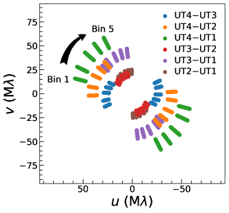
Figure 2: $uv$ coordinates of the binned data. Each coloured stripe spans the averaged $uv$ coverage of a given baseline over the spectral range. From bin 1 to bin 5, the $uv$ coverage of the 6 baselines rotates clockwise.

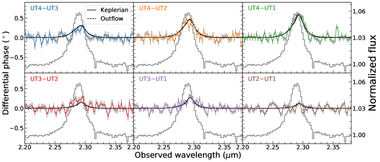
Figure 3: Averaged differential phase spectra (coloured) and the normalised Br$\gamma$ spectrum (grey histogram) for IRAS 09149$-$6206. Solid and dashed black curves show the differential phase spectra of the best-fit BLR models (see Sec. 4). For the purpose of presentation, we average all of the data in each baseline. BLR modelling, however, was done on the five bins based on $uv$ coverage as shown in Fig. 2. The same Br$\gamma$ spectrum is displayed in all of the panels.

2.3 The averaged differential phase

The phase of the pipeline reduced visibility shows significant ($\gtrsim 1{\mbox{${}^{\circ}$}}$) instrumental features across the spectral band, which also varies between exposures. As discussed in Appendix A, we find that the instrumental features primarily consist of two components. A variable component is introduced by the dispersion of the air in the non-vacuum delay line of the VLTI, while a stable component is likely generated inside the cryostat of GRAVITY. Crucially, the variable component has a stable profile as a function of wavelength and only the total amplitude changes with each exposure. We remove these systematic features by fitting and subtracting a simple instrumental phase model – a stable component plus a fixed phase profile with a variable amplitude. Using calibrator star data, we demonstrate that the systematic uncertainty of our flattening method reaches $\lesssim 0.05$^∘ across most of the wavelength coverage (2.05–2.40 $\mu$m) of GRAVITY.

When we remove the residual instrumental features described above, we also mask out the wavelength range (2.25–2.35 $\mu$m) where the broad Br$\gamma$ line in IRAS 09149$-$6206 dominates. The mask does not affect the flattening (see Appendix A). Similarly, the uncertainty of the differential phase is estimated from the RMS of the flattened phase at 2.05–2.40 $\mu$m, masking the wavelength range of the broad Br$\gamma$. In addition, we also fit a 2nd order polynomial function locally around the Br$\gamma$ line, avoiding the line core (2.20–2.27 $\mu$m and 2.31–2.38 $\mu$m), to further flatten the phase around the line. This is necessary because IRAS 09149$-$6206 shows a slight positive phase gradient across the broad emission lines, including Br$\gamma$ (2.2896 $\mu$m), Br$\delta$ (2.0551 $\mu$m), and Pa$\alpha$ (1.9821 $\mu$m). Without this step, the pipeline would create a phase dip around the blue wing of the Br$\gamma$ line because it derives the phase reference without considering the scientific signal. Using the calibrator data, we find that the additional flattening procedure does not increase the noise with respect to the systematic uncertainty ($\sim 0.05{\mbox{${}^{\circ}$}}$; Appendix A). Finally, as shown in Fig. 2, we split the data collected across the three years into 5 angular $uv$ bins in order to minimise smearing of the phase signal. We then averaged the differential phase in each spectral bin, weighted by the uncertainty, resulting in total integration times for each bin between 1.3 and 1.8 hours. The full set of binned differential phase spectra can be seen in Appendix D while in Fig. 3 we show the averaged differential phase spectra for each baseline. The six baselines have different orientations and $uv$ distances (Fig. 2). The longer baselines are more sensitive to the small scale signal. Therefore, the signals measured by different baselines behave differently.

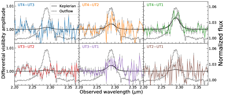
Figure 4: Averaged differential visibility amplitude spectra (coloured) and the normalised Br$\gamma$ spectrum (grey histogram) for IRAS 09149$-$6206. There is a clear positive differential visibility amplitude signal in the UT4$-$UT1 spectrum, which follows well the line profile. Solid and dashed black curves show the differential visibility amplitude of the best-fit BLR models (see Sec. 4.4). Several channels with large scatter at $>2.3\,{\mbox{$\mu$m}}$ are masked for clarity. The same Br$\gamma$ spectrum is displayed in all of the panels.

2.4 The differential visibility amplitude

To produce the differential visibility amplitude, we fit and divide out a 2nd order polynomial from the pipeline reduced SC visibility amplitude while masking the Br$\gamma$ line region. The uncertainty is estimated from the RMS of the resulting normalised continuum channels. We then average the differential amplitudes from each exposure together, weighted by their inverse variance, and the final uncertainty is calculated by propagating the individual exposure uncertainties. Instead of $uv$ binning, we simply average all exposures for a single baseline together, since the signal in the differential visibility amplitude is much weaker than the differential phase. As shown in Fig. 4, the differential visibility amplitude of UT4$-$UT1 is well above 1 and follows the profile of the emission line. The small dip in the differential visibility amplitude signal around the central wavelength of the line may be due to the narrow Br$\gamma$ component; but it does not affect our analysis because it is barely significant compared to the noise level.

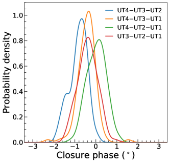
Figure 5: Kernel density estimates for the closure phase distribution from the FT data of IRAS 09149$-$6206. The closure phase distributions for the four triangles are consistent with 0^∘.

2.5 Continuum visibility from the fringe tracker

The fringe tracker kept a record of fringe measurements at 300 Hz throughout the exposures. There are six spectral channels across $K$ band. The visibility amplitude and closure phases are important to constrain the continuum emission. In Fig. 5, we plot the closure phase distribution for the four triangles. All distributions are consistent with an average closure phase between $-1{\mbox{${}^{\circ}$}}$ and 0^∘.

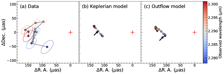
Figure 6: Best-fit centroids to the differential phases of (a) observed data of IRAS 09149$-$6206, (b) the best-fit Keplerian model described in Sec. 4.2, and (c) the best-fit outflow model described in Sec. 4.3. The colour code represent the wavelength of the channels around the centre of the Br$\gamma$ line. The coloured ellipses around each centroid in panel (a) represents the 68% (1 $\sigma$) credible intervals of the uncertainty. The red plus sign at the origin represents the photocentre of the continuum. The black arrows in panel (b) and (c) indicate the origin of the BLR according to the inferred offset of the models.

3 Locating the Broad Line Region

The differential visibility amplitude spectra provide direct evidence that the BLR has been unambiguously detected. The signal is especially clear in the UT4$-$UT1 baseline shown in Fig. 4, where the differential visibility amplitude significantly increases across the BLR line profile. The channels dominated by broad Br$\gamma$ emission display higher visibility amplitude, hence smaller size, than those dominated by the continuum (see Sec. 4.4). Consistent with GC20a, this indicates that the BLR is more compact than the near-infrared continuum, which traces the hot dust distribution around the AGN. IRAS 09149$-$6206 also shows a strong differential phase signal primarily in the UT4$-$UT2 and UT4$-$UT1 baselines. Remarkably, as is apparent in Fig. 3, the signal is also entirely positive and peaks near the line centre, which is different from the ‘S-shape’ seen in 3C 273 (GC18) that crosses zero at the line centre.

A differential phase following the shape of the line profile is expected for a constant phase difference between the hot dust continuum and the Br$\gamma$ emission. Both sources are marginally resolved, which is strongly supported by the $\sim 0{\mbox{${}^{\circ}$}}$ closure phase in Fig. 5. This means that to first order a phase difference measures an offset in photocentre position. The phase signal caused by this offset, we hereafter refer to as the ‘continuum phase’. By construction, the differential phase data are referenced to the photocentre position of the hot dust continuum. Hence, we have the differential phase, $\Delta\phi_{\lambda}=-2\pi\,[f_{\lambda}/(1+f_{\lambda})]\,\@vec{u}\cdot\@vec{x}_{\mathrm{BLR},\lambda}$, where $f_{\lambda}$ is the line flux at wavelength $\lambda$ relative to a continuum level of unity, $\@vec{u}$ is the $uv$ coordinate of the baseline, and $\@vec{x}_{\mathrm{BLR},\lambda}$ is the coordinate of the photocentre w.r.t. the centroid of the continuum (see Appendix B for details). Fitting the photocentre coordinate of each channel to the differential phase data of 30 baselines (6 baselines $\times$ 5 angular bins), we can reconstruct the photocentres of the IRAS 09149$-$6206 Br$\gamma$ line emission.

The result in Fig. 6 (a) shows a systematic offset of the BLR photocentres from the origin by $\sim 120\,\mu$as to the east. Moreover, there is clear evidence for a velocity gradient that is nearly perpendicular to the offset: the blueshifted channels lie predominantly to the south of the red-shifted channels. While the separation between individual channels is only moderate given the uncertainties, the general gradient from North to South appears robust. Following GC18, we estimate the significance of the offset between the blue and red channels with an F-test, comparing the null hypothesis that the phase signal is produced by a single position of the unresolved BLR with the hypothesis that the blue and red channels are at two distinct positions. Using the same channels as shown in Fig. 6 (a) (6 blue channels $<2.2896\,{\mbox{$\mu$m}}$ and 5 red channels $>2.2896\,{\mbox{$\mu$m}}$), we find the red-blue photocentre offset is at $>8\,\sigma$ significance. If we use only alternate channels, in order to avoid the impact of possible data correlation, the same method still yields a significance $>5\,\sigma$. According to this simple model, the average photocentre displacement on sky is $33\pm 8\,\mu$as, which can be considered as the lower limit of the separation of the photocentres.

This red-blue photocentre displacement, while model independent, is only a lower limit to the true physical BLR size. To measure the physical size and constrain the BLR kinematics, a model is required. We adopt a flexible model, with a full differential phase (see also Appendix B),

$$\Delta\phi_{\lambda}=[f_{\lambda}/(1+f_{\lambda})]\,(\phi_{\mathrm{BLR},\lambda}-2\pi\,\@vec{u}\cdot\@vec{x}_{\mathrm{o}}),$$ (1)

where $\@vec{x}_{\mathrm{o}}$ is the coordinate of the origin of the BLR with respect to the centroid of the continuum. This velocity-independent photocentre offset could for example result from asymmetric structure in the continuum, or a physical offset between the BLR and hot dust continuum. The kinematic model described in the next section provides the velocity-dependent phase $\phi_{\mathrm{BLR},\lambda}$ of the BLR itself.

4 Rotation versus Outflow in the Broad Line Region

The GRAVITY measurements of the line and phase profile for 3C 273 were modelled with a simple model consisting of a symmetric distribution of clouds in circular orbits, which fitted those data very well GC20a. In that particular case, the model is supported by the symmetric profile of the broad Pa$\alpha$ emission line, as well as the fact that the orientation of the radio jet is almost perfectly perpendicular to the gradient of the photocentres. With more limited knowledge available for IRAS 09149$-$6206, it is not clear a priori whether the velocity gradient we observe reflects rotational or radial motion of the BLR. As such, we adopt a flexible BLR model with a generalised prescription of the BLR dynamics (Pancoast et al., 2014a). The specific code we use here was developed by Stock (2018) and already adopted in the analysis of 3C 273 (GC18).

Following a general description of the model and its various parameters in Sec. 4.1, we compare the fits for two different implementations, allowing in both cases for an offset between the continuum and the BLR as discussed above. For the first case, in Sec. 4.2, we reduce the model to circular orbits as was applied in the case of 3C 273. For the second case, in Sec. 4.3, we apply the full model, allowing for radial motions. Sec. 4.4 then checks the consistency of both models with the observed differential visibility amplitudes. Finally, a comparison of the fits in Sec. 4.5 shows that the goodness of fit does not indicate a preference based on the data alone, and it is instead the astrophysical implication that leads to a preference of one model.

$R_{\rm BLR}$	Mean radius of the BLR	$\mathrm{LogUniform(10^{-4},10\,pc)}$
$F$	Minimum radius of the BLR in units of $R_{\rm BLR}$	$\mathrm{Uniform(0,1)}$
$\beta$	Unit standard deviation of BLR radial profile	$\mathrm{Uniform(0,2)}$
$\theta_{\mathrm{o}}$	Angular thickness measured from the mid-plane	$\mathrm{Uniform(0,\pi/2)}$
$i$	Inclination angle	$\mathrm{Uniform}(\cos{i(0,\pi/3)})$
$PA$	Position angle of the line of nodes on sky (east of north)	$\mathrm{Uniform(0,2\pi)}$
$\kappa$	Anisotropy of the cloud emission	$\mathrm{Uniform(-0.5,0.5)}$
$\gamma$	Clustering of the clouds at the edge of the disk	$\mathrm{Uniform(1,5)}$
$\xi$	Mid-plane transparency	$\mathrm{Uniform(0,1)}$
$M_{\mathrm{BH}}$	Black hole mass	$\mathrm{LogUniform}(10^{5},10^{10}\,M_{\odot})$
$f_{\mathrm{ellip}}$	Fraction of clouds in bound elliptical orbits	$\mathrm{Uniform(0,1)}$
$f_{\mathrm{flow}}$	Flag for specifying inflowing or outflowing orbits	$\mathrm{Uniform(0,1)}$
$\theta_{\mathrm{e}}$	Angular location for radial orbit distribution	$\mathrm{Uniform(0,\pi/2)}$
$\sigma_{\rho,\mathrm{circ}}$	Radial standard deviation for circular orbit distribution	$\mathrm{LogUniform(0.001,0.1)}$
$\sigma_{\Theta,\mathrm{circ}}$	Angular standard deviation for circular orbit distribution	$\mathrm{LogUniform(0.001,1)}$
$\sigma_{\rho,\mathrm{radial}}$	Radial standard deviation for radial orbit distribution	$\mathrm{LogUniform(0.001,0.1)}$
$\sigma_{\Theta,\mathrm{radial}}$	Angular standard deviation for radial orbit distribution	$\mathrm{LogUniform(0.001,1)}$
$\sigma_{\mathrm{turb}}$	Normalized standard deviation of turbulent velocities	$\mathrm{LogUniform(0.001,0.1)}$
$\lambda_{\mathrm{emit}}$	Central wavelength of the emission line	$\mathrm{Norm(2.2896,0.002\,{\mbox{$\mu$m}})}$
$f_{\mathrm{peak}}$	Peak flux of the normalized line profile	$\mathrm{Uniform(0.05,0.065)}$
$(x_{\mathrm{o}},y_{\mathrm{o}})$	Offset of the origin of the BLR	$\mathrm{Uniform(-1,1\,\mathrm{mas})}$

Table 2: Parameters of the BLR model with definitions, priors, and units where appropriate (all angles are in radians). The priors for most parameters are specified here in one of two ways. Uniform(min,max) denotes uniform sampling over the range specified. LogUniform(min,max) indicates that the logarithm of the parameter is sampled uniformly over the logarithm of the range. The prior for the inclination angle ($i$) is set between 0 and $\pi/2$ so that $\cos{i}$ is uniformly sampled between 0 and 1. The prior for the central wavelength of the emission line ($\lambda_{\mathrm{emit}}$) follows a Gaussian distribution centered at 2.2896 $\mu$m and with a standard deviation 0.002 $\mu$m.

4.1 The generalised BLR model

The generalised BLR model was developed by Pancoast et al. (2014a, P14), with the original purpose to model the spectra and light curves from RM campaigns. The P14 model describes the BLR as a large number of non-interacting clouds and includes a large number of parameters, summarised in Table 2, that define the position and motion of each of those clouds. Below, we briefly describe how these affect the geometry and dynamics of the model.

The first set of parameters defines the locations of the clouds. Their distances from the black hole are given as

$$r=R_{\mathrm{S}}+F\,R_{\mathrm{BLR}}+g\,(1-F)\,\beta^{2}\,R_{\mathrm{BLR}},$$ (2)

where $R_{\mathrm{S}}=2G{\mbox{$M_{\mathrm{BH}}$}}/c^{2}$ is the Schwarzschild radius, $R_{\mathrm{BLR}}$ is the mean radius, $F=R_{\mathrm{min}}/R_{\mathrm{BLR}}$ is the fractional inner radius, $\beta$ is the shape parameter, and $g=p(x|1/\beta^{2},1)$ is drawn randomly from a Gamma distribution

$$p(x|a,b)=\frac{x^{a-1}e^{-x/b}}{\Gamma(a)\,b^{a}},$$ (3)

where $\Gamma(a)$ is the gamma function. Using a shape parameter in this way provides enough flexibility to reproduce several qualitatively different radial distributions, namely a Gaussian ($0<\beta<1$), exponential ($\beta=1$), or heavy-tailed ($1<\beta<2$) profile. The angular distribution of the clouds is given by

$$\theta=\arccos{(\cos{{\mbox{$\theta_{\mathrm{o}}$}}}+(1-\cos{{\mbox{$\theta_{\mathrm{o}}$}}})\times U^{\gamma})},$$ (4)

where $\theta_{\mathrm{o}}$ is the angular thickness of the distribution (defined as the angle between the mid-plane and the upper edge of the distribution) and $U$ is a random number drawn uniformly between 0 and 1. Setting $\gamma>1$ concentrates more clouds closer to the maximum angular height $\theta_{\mathrm{o}}$. The structure is viewed at an inclination angle $i$ (where $i=0^{\circ}$ is defined to be face-on) and rotated in the plane of the sky so that the line of nodes is at position angle $PA$ (measured east of north). A weight is assigned to each cloud to represent the relative strength of its emission, and is defined as

$$w=0.5+\kappa\cos\phi,$$ (5)

where $\kappa$ is a parameter in the range ($-0.5$, 0.5) reflecting any anisotropy of the emission, and $\phi$ is the angle between the line of sight from the cloud to the observer and to the central ionising source. The mid-plane transparency is modelled using the parameter $\xi$ which controls the fraction of clouds located behind the equatorial plane. If $\xi=1$ then the clouds are evenly distributed on either side of the equatorial plane, while $\xi=0$ means that all the clouds are in front of it.

The remainder of the parameters define the kinematics of the clouds, under the assumption that their motions are governed entirely by the gravitational potential of the black hole. A fraction, $f_{\mathrm{ellip}}$, of the clouds are put on bound elliptical orbits. The rest are placed on much more elongated orbits, which are dominated by radial motion. A single parameter, $f_{\mathrm{flow}}$, is used as a binary switch to control whether the radial motion is inflow ($0<f_{\mathrm{flow}}<0.5$) or outflow ($0.5<f_{\mathrm{flow}}<1$).

For the bound elliptical orbits, radial and tangential velocities, $v_{\mathrm{r}}$ and $v_{\phi}$, are drawn randomly from a distribution centred on the point $\{0,{\mbox{$v_{\mathrm{circ}}$}}\}$ in the $v_{\mathrm{r}}$–$v_{\phi}$ plane (see Fig. 2 in Pancoast et al. 2014a), where ${\mbox{$v_{\mathrm{circ}}$}}=\sqrt{G{\mbox{$M_{\mathrm{BH}}$}}/r}$ is the circular velocity. The distribution itself follows an ellipse in the $v_{\mathrm{r}}$–$v_{\phi}$ plane that is defined as

$$\frac{v_{\mathrm{r}}^{2}}{2v_{\mathrm{circ}}^{2}}+\frac{v_{\phi}^{2}}{v_{\mathrm{circ}}^{2}}=1,$$ (6)

and is defined to be a Gaussian with standard deviation $\sigma_{\Theta,\mathrm{circ}}$ along the ellipse and $\sigma_{\rho,\mathrm{circ}}$ perpendicular to it.

Because the ellipse naturally connects points around $\{0,{\mbox{$v_{\mathrm{circ}}$}}\}$ corresponding to circular orbits, with points around $\{\pm\sqrt{2}{\mbox{$v_{\mathrm{circ}}$}},0\}$ corresponding to highly elongated orbits, the orbits dominated by radial motion can be defined in a similar way. In this case, there is an additional parameter $\theta_{\mathrm{e}}=\arctan{(|v_{\phi}/v_{\mathrm{r}}|)}$ that defines the angular location around the ellipse where the distribution is centred. If $\theta_{\mathrm{e}}$ is close to $\pi/2$, the orbit distribution is centred around $\{0,{\mbox{$v_{\mathrm{circ}}$}}\}$ exactly as for the bound elliptical orbits and there is very little inflow or outflow. As $\theta_{\mathrm{e}}$ approaches 0, the centre of the distribution shifts to $\{\pm\sqrt{2}{\mbox{$v_{\mathrm{circ}}$}},0\}$ where orbits are dominated by radial motion at the escape velocity. The distribution is defined around the point on the ellipse corresponding to $\theta_{\mathrm{e}}$ as a Gaussian with standard deviation $\sigma_{\Theta,\mathrm{radial}}$ along the ellipse and $\sigma_{\rho,\mathrm{radial}}$ perpendicular to it. The units of $\sigma_{\rho,\mathrm{circ}}$ and $\sigma_{\rho,\mathrm{radial}}$ are given in terms the circular velocity of the clouds, while $\sigma_{\Theta,\mathrm{circ}}$ and $\sigma_{\Theta,\mathrm{radial}}$ are given as a fraction of $\pi$. The last velocity component is a random velocity $v_{\mathrm{turb}}$ describing the macroturbulence. This is randomly sampled from a Gaussian distribution with standard deviation $\sigma_{\mathrm{turb}}v_{\rm circ}$, and added to the line-of-sight velocity of each cloud.

The full relativistic Doppler effect and gravitational redshift are also taken into account in generating the spectrum and differential phases. For each cloud, the intrinsic line width is assumed to be negligible. The wavelength of the line is shifted from $\lambda_{\mathrm{emit}}$ to $\lambda_{\mathrm{obs}}$ (both in the observed frame) by

$$\lambda_{\mathrm{obs}}=\lambda_{\mathrm{emit}}\frac{1-\frac{v_{\mathrm{los}}}{c}}{\sqrt{1-\frac{v^{2}}{c^{2}}}}\frac{1}{\sqrt{1-\frac{R_{\mathrm{s}}}{r}}},$$ (7)

where $v_{\mathrm{los}}$ is the total line-of-sight velocity and $v$ is the total velocity. Finally, we bin the clouds in the spectral channels according to their $\lambda_{\mathrm{obs}}$ and sum their weights to derive the normalised line profile. The profile is then scaled by $f_{\mathrm{peak}}$, so that it has the same normalisation as the continuum. The projected coordinates perpendicular to the line of sight are averaged in each bin according to the cloud weights to derive the photocentre of each spectral channel. The differential phase is then calculated with Equation (1) with,

$$\phi_{\mathrm{BLR},\lambda}=-2\pi\,\frac{f_{\lambda}}{1+f_{\lambda}}\@vec{u}\cdot\left(\frac{\sum_{i}w_{i}\@vec{x}_{i}}{\sum_{i}w_{i}}\right),$$ (8)

where $w_{i}$ and $\@vec{x}_{i}$ are the weight and coordinate of the $i$th cloud of the BLR with $\lambda_{\mathrm{obs}}$ within the wavelength channel $\lambda$.

Our prior assumptions on all these parameters, as given in Table 2, generally follow the choices of Pancoast et al. (2014a). The main exception is the inclination angle, which we require to be below 50^∘, because the BLR of a type 1 AGN is expected to be relatively face-on. For the prior on $\lambda_{\mathrm{emit}}$, we adopt a Gaussian distribution centred at 2.2896 $\mu$m based on the redshift measured by Perez et al. (1989). The standard deviation of the Gaussian distribution is 0.002 $\mu$m, which is the width of the spectral channel and the equivalent $\sigma$ of the line spread function for the GRAVITY science spectrograph. Three additional parameters that we include are the peak flux $f_{\rm peak}$ of the emission line normalised to the continuum, and the offset $\{x_{\rm o},y_{\rm o}\}$ for the origin of the BLR. The prior range adopted for $f_{\mathrm{peak}}$ is 0.05–0.065. The offset of the BLR, $\{x_{\mathrm{o}},y_{\mathrm{o}}\}$, is allowed to vary by up to $-1$ to 1 mas in both directions.

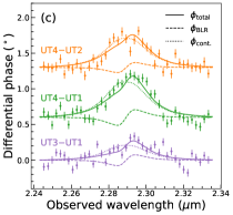
Figure 7: (a) The cloud distribution of the best-fit Keplerian model. Each circle represents one cloud, colour-coded by the line-of-sight velocity. The zero velocity is defined at the best-fit $\lambda_{\mathrm{emit}}$. The red plus sign at the origin represents the photocentre of the continuum. The orientation of the model is consistent with the observed photocentre gradient. (b) The observed averaged differential phase from UT4$-$UT2, UT4$-$UT1, and UT3$-$UT1 after removing the ‘continuum phase’ signal (blue) compared to the averaged differential phase from the best-fit BLR model (red). These baselines were chosen since they contain the strongest ‘S-shape’ signal. Above, the observed line profile (black) is compared with the model line profile (red). The residual of the spectrum subtracting the model line profile is displayed in the lower panel. The left $y$ axis corresponds to the averaged differential phase, while the right $y$ axis corresponds to the line profile. (c) The differential phase data and the best-fit models (solid lines) of the three baselines that show the strongest signal of the BLR component (dashed lines). The phase in panel (b) is calculated by averaging the phases of these three baselines after subtracting the best-fit continuum phases (dotted lines).

4.2 Model with Circular Keplerian Rotation

The P14 model described above can easily be reduced to circular Keplerian rotation. Setting $\kappa=0$ and $\xi=1$ ensures that the clouds are equally weighted (i.e. emitting isotropically) and are distributed uniformly above and below the equatorial plane. Instead of using Equation (4) to determine the initial angular distribution of the clouds, the circular Keplerian model distributes them uniformly between 0 and $\theta_{\mathrm{o}}$ (GC18). To produce bound circular orbits, we set $f_{\mathrm{ellip}}=1$, $\sigma_{\rho,\mathrm{circ}}=0$, and $\sigma_{\Theta,\mathrm{circ}}=0$. Finally, setting $\sigma_{\mathrm{turb}}=0$ ensures that there is no additional turbulence. We refer to this model as the “Keplerian model”, hereafter, for simplicity.

The flux and differential phase spectra of IRAS 09149$-$6206 are fit reasonably well by the Keplerian model, as shown in Fig. 3 for the averaged bins (see also Fig. 17 for the individual bins). The most prominent phase signals in the UT4$-$UT2, UT4$-$UT1, and UT3$-$UT1 baselines are primarily due to the continuum phase produced by the offset between the BLR and the centre of the continuum emission. For this model, the BLR is $\sim 120\,\mu$as east of the continuum centre. The cloud distribution of the model is shown in Fig. 7 (a), and the corresponding photocentres in Fig. 6 (b) are qualitatively consistent with those reconstructed from the data. The best fitting parameters summarised in Table 3 indicate that a rather face-on disk with $i\approx 21{\mbox{${}^{\circ}$}}$ is favoured by the data, which is consistent with the inclination found from an upcoming dust reverberation study (S. Hönig et al. in preparation). A low inclination is consistent with the Seyfert 1 classification and, as one would expect, low inclinations are generally inferred when fitting RM data of other objects. The disk is also very thick, with ${\mbox{$\theta_{\mathrm{o}}$}}\approx 71{\mbox{${}^{\circ}$}}$. Grier et al. (2017a) have suggested that, when fitting RM data, the thickness $\theta_{\mathrm{o}}$ is always similar to the inclination angle $i$, due to degeneracy between the two quantities. Interferometry breaks this degeneracy. Our derived values for these parameters are significantly different, and the posterior distributions in Fig. 18 show no particular coupling. The mean radius of $R_{\mathrm{BLR}}=65\,\mu$as corresponds to 0.075 pc. The posterior distributions in Fig. 18 indicate that there is some degeneracy between BLR radius, black hole mass, and the inclination angle, which is consistent with previous studies (Rakshit et al. 2015; GC18). Although the inferred line centre $\lambda_{\mathrm{emit}}=2.2892\,{\mbox{$\mu$m}}$ corresponds to a velocity offset of $\Delta v_{\mathrm{BLR}}=-56\,\mathrm{km\,s^{-1}}$ with respect to the systemic velocity from the [O III] rotation curve (Perez et al., 1989), the uncertainty of $\Delta v_{\mathrm{BLR}}$ is large enough that the modelled line centre is fully consistent with it.

In order to display the phase signal specific to the BLR, we subtract the best-fit continuum phase from the data in the three longest baselines (UT4$-$UT2, UT4$-$UT1, and UT3$-$UT1) as shown in Fig. 7 (c), and then average them. The residual BLR signal, shown in Fig. 7 (b), exhibits the expected ‘S-shape’ profile for a rotating structure. Based on the analysis in Appendix A, and taking into account that several baselines were combined, the uncertainty of this phase is expected to be below 0.03^∘ per spectral channel. As such, even though the $\sim 0.1{\mbox{${}^{\circ}$}}$ BLR signal is several times weaker than the continuum phase signal, it remains a significant detection. We note that the ‘S-shape’ profile is due to specifically fitting with the Keplerian model. The significance of the BLR phase signal is constrained model-independently with the reconstructed photocentres (Sec. 3). Finally, we also need to consider the fit to the spectral line profile. The Keplerian model is only able to generate a symmetric line profile, which also means that $\lambda_{\mathrm{emit}}$ is close to the wavelength of the peak of the line profile. However, the observed line profile of IRAS 09149$-$6206 is slightly asymmetric. As such, although the line profile is reasonably well matched by the model, a difference between the model and data, especially in the blue wing (e.g., 2.24–2.29 $\mu$m), is apparent in Fig. 7 (b). This issue is addressed in the next Section.

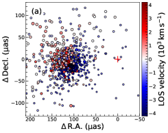
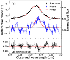
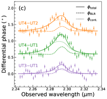
Figure 8: (a) The cloud distribution of the best-fit outflow model. The symbols and lines are the same as for Fig. 7, except that in panel (a) the sizes of the circles scale with the weight of the cloud.

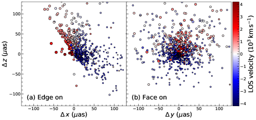
Figure 9: The (a) edge-on and (b) face-on view of the best-fit outflow model, except that the PA is adjusted to 180^∘ and the BLR is moved back to the origin of the plot for clarity. In both panels, the colour coding represents the line-of-sight velocity for each cloud. Following Pancoast et al. (2014a, b), $\Delta x$ is along the line of sight, $\Delta y$ is the direction of the right ascension, and $\Delta z$ is the direction of declination.

4.3 Model including Radial Motion

Parameters	Circular Keplerian model	Outflow model
$R_{\mathrm{BLR}}\,(\mu\mathrm{as})$	$65_{-39}^{+30}$	$50_{-11}^{+38}$
$R_{\mathrm{min}}\,(\mu\mathrm{as})$	$8.3_{-7.4}^{+13.1}$	$6.8_{-5.0}^{+7.5}$
$\beta$	$1.17_{-0.33}^{+0.30}$	$1.27_{-0.32}^{+0.17}$
$\theta_{\mathrm{o}}\,(^{\circ})$	$71_{-27}^{+16}$	$61_{-20}^{+20}$
$i\,(^{\circ})$	$21_{-8}^{+20}$	$35_{-10}^{+13}$
PA (∘ E of N)	$130_{-34}^{+29}$	$219_{-37}^{+27}$
$\kappa$	…	$-0.32_{-0.17}^{+0.44}$
$\gamma$	…	$1.27_{-0.20}^{+2.40}$
$\xi$	…	$0.05_{-0.04}^{+0.30}$
Offset ($\mu$as)	$\left(121.6_{-9.7}^{+6.5},4.5_{-8.6}^{+8.4}\right)$	$\left(109.2_{-21.8}^{+11.5},-13.9_{-17.4}^{+12.3}\right)$
$\log\,({\mbox{$M_{\mathrm{BH}}$}}/M_{\odot})$	$8.06_{-0.57}^{+0.41}$	$7.70_{-0.18}^{+0.41}$
$f_{\mathrm{ellip}}$	1	$0.19_{-0.17}^{+0.35}$
$f_{\mathrm{flow}}$	…	$0.71_{-0.20}^{+0.26}$
$\theta_{\mathrm{e}}$	…	$5.0_{-4.3}^{+22.9}$
$\log\,\sigma_{\mathrm{turb}}$	0	$-1.87_{-1.04}^{+0.80}$
$\Delta v_{\mathrm{BLR}}\,(\mathrm{km\,s^{-1}})$	$-56_{-67}^{+78}$	$380_{-356}^{+208}$
$\chi_{\mathrm{r}}^{2}$	1.39	1.38
$\ln\,K$	0	$7.1\pm 0.2$
$\Delta$ AIC	0	-12.6
$\Delta$ BIC	0	44.0

Table 3: The inferred maximum a posteriori value and central 95% credible interval for the modelling of the spectrum and differential phase of IRAS 09149$-$6206. $\Delta v_{\mathrm{BLR}}$ is the difference between the velocity derived from the best-fit $\lambda_{\mathrm{emit}}$ and the systemic velocity based on the [O III] line (Perez et al., 1989). $\chi_{\mathrm{r}}^{2}$ is the reduced $\chi^{2}$ of the models with the best-fit parameters. The Bayes’ factor, AIC, and BIC are relative to the Keplerian model.

To be able to fit the asymmetries in the emission line profile, we apply the full P14 model. The best fitting parameters of the P14 model (Table 3) include $f_{\mathrm{ellip}}\approx 0.2$ indicating that the majority of the clouds are on orbits with a dominant radial component, $\theta_{\rm e}\approx 5{\mbox{${}^{\circ}$}}$ indicating that the orbits are sufficiently elongated that the radial motion is very close to the escape velocity, and $f_{\mathrm{flow}}>0.5$ indicating that this radial motion is outward. Together, these indicate that, although it is not required a priori, the configuration of the model preferred by the data is very much dominated by outflow. As such, hereafter we call this the ‘outflow model’.

As before, the phase signals shown in Fig. 3 (see also Fig. 19 for the individual bins) are dominated by the continuum phase. The BLR offset of $\sim 110\,\mu$as, which can be seen in Fig. 8 (a), is statistically consistent with that of the Keplerian model. The modest difference is due to the different BLR phase signals (Fig. 8(b)). The orientation and gradient of the photocentres in Fig. 6 (c), are also consistent with the data. The outflow model indeed better fits the line profile compared to the Keplerian model. No systematic residual is seen in Fig. 8(b), especially in the blue wing. Because the two models fit the differential phase data equally well, as shown in Fig. 3, the total goodness of fit for the two models are nearly indistinguishable (Sec. 4.5).

The mean radius of $R_{\mathrm{BLR}}=50\,\mu$as is slightly smaller than, but statistically consistent with, that of the Keplerian model. The cloud radial distribution given by $\beta=1.27$ prefers to be exponential or heavy-tailed, with a small inner radius of $R_{\mathrm{min}}=6.8\,\mu$as. The model has $\mathrm{PA}\approx 219{\mbox{${}^{\circ}$}}$, which is 90^∘ different from Keplerian model. The reason is simply that the BLR kinematics, and hence the orientation of the velocity gradient, are now dominated by radial motion rather than rotation. This model also prefers anisotropic emission from the clouds, with $\kappa=-0.32$ indicating that line emission is stronger from the inner illuminated side of the clouds and hence the far side of the distribution, similar to many of the results inferred from RM data. The parameter $\sigma_{\mathrm{turb}}=0.013$ implies that additional macroscopic turbulence is not significant. As for the Keplerian model, $\theta_{0}\sim 61$^∘ indicates that the cloud trajectories are distributed over a wide range of angles from the mid-plane. We also note, similarly to the Keplerian model, that the thickness and inclination have somewhat different values, and there is no evidence for degeneracy between them in the posterior distributions shown in Fig. 20. Indeed, except for the greater thickness of the BLR in IRAS 09149$-$6206, the configuration is rather similar to that inferred from RM data for Arp 151 (Pancoast et al., 2014b), Zw 229$-$015 (Williams et al., 2018), or Mrk 142 (Li et al., 2018). Finally, the best fit line centre is $\lambda_{\mathrm{emit}}=2.2923\,{\mbox{$\mu$m}}$ which corresponds to an offset $\Delta v_{\mathrm{BLR}}=380\,\mathrm{km\,s^{-1}}$ from the systemic velocity. A discussion of whether this is physically plausible is deferred to Sec. 4.5.

One of the most important aspects of this model is that the differential phase of the BLR component is very different to the ‘S-shape’ seen in the Keplerian model. It is clear from Fig. 8 (b) that the continuum subtracted phase data fitted by the BLR model is dominated by a positive signal on the red-shifted side of the line profile. Fig. 8 (c) illustrates the decomposition of the BLR phase and continuum phase components. The asymmetric BLR phase signal is produced by two main effects: (i) The BLR kinematics are dominated by outflow (as discussed above) and (ii) $\xi\approx 0$ means that the mid-plane is opaque. The impact of this second effect is discussed below in the context of the distribution and motions of the clouds.

The edge-on and face-on views of the cloud distribution presented in Fig. 9 can shed more light on the role of the mid-plane obscuration in generating the positive phase signal. The edge-on view clearly shows that the cloud distribution extends far above the mid-plane because ${\mbox{$\theta_{\mathrm{o}}$}}\approx 60{\mbox{${}^{\circ}$}}$; while $\xi\approx 0$ means that the mid-plane obscuration is so strong that there are few clouds below it. As discussed above, our model is significantly dominated by outflowing clouds. The blue-shifted clouds are on the near side towards the observer, while the red-shifted clouds are on the far side. In addition, the anisotropy parameter $\kappa\approx-0.3$ means that the weighting applied to clouds on the far side is much larger than for the near side. This effect is indicated in the figure by the size of the circles representing the clouds: on the side nearer the observer, the circles are much smaller than those on the far side. The mid-plane obscuration and inclination angle together mean that, as is apparent in Fig. 8 (a), the blue-shifted clouds are distributed fairly symmetrically around the centre of the BLR. This means that their photocentre is close to the BLR centre and the corresponding differential phases are close to 0^∘. In contrast, the red-shifted clouds are primarily located to the northeast of the BLR centre, so the corresponding red-shifted channels show significant differential phase signal. As a result, as shown in Fig. 6, the origin of the BLR coincides with the blue-shifted channels instead of with the channel associated with the line peak.

4.4 Model prediction of the differential visibility amplitude

The measured differential visibility amplitude is useful to provide an independent check of the BLR model fits. The differential visibility amplitude ($V_{\rm diff}$) is derived by normalising the total visibility amplitude with the visibility amplitude of the continuum $V_{c}$. In each spectral channel $\lambda$, this is

$$V_{\mathrm{diff}}(\lambda)=\frac{1+f_{\lambda}V_{\mathrm{BLR}}(\lambda)/V_{c}(\lambda)}{1+f_{\lambda}},$$ (9)

where $V_{\mathrm{BLR}}$ is the visibility amplitude of the line emission of the BLR. At the wavelength of the line emission, one will find $V_{\mathrm{diff}}>1$ if $V_{\mathrm{BLR}}/V_{c}>1$, this is if the BLR emission is more compact than the continuum emission. This can be seen in Fig. 4, in particular for the UT4$-$UT1 baseline. Similar results have been reported for 3C 273 (GC18) and PDS 456 (GC20a).

The visibility amplitude of the continuum emission of IRAS 09149$-$6206 has already been studied in GC20a. Using the visibility amplitude from the fringe tracker channel and the differential visibility from the science channel, we derived consistent FWHM sizes $0.54\pm 0.05$ mas and $0.64\pm 0.06$ mas, respectively, for a circular Gaussian profile. This indicates that the continuum emission is only marginally resolved. For consistency, we adopt a Gaussian profile with $\mathrm{FWHM}=0.6\,\mathrm{mas}$ to calculate

$$V_{c}(\lambda)=\exp{\left(-\frac{(\pi\,\mathrm{FWHM})^{2}(u^{2}+v^{2})}{4\ln 2}\right)}.$$ (10)

Following Waisberg et al. (2017), we calculate $V_{\mathrm{BLR}}$ from the Keplerian and outflow models from the second moment of the source emission,

$$V_{\mathrm{BLR}}(\lambda)\approx 1-\frac{2\pi^{2}}{\mu_{00,\lambda}}\left(u^{2}\tilde{\mu}_{20,\lambda}+v^{2}\tilde{\mu}_{02,\lambda}+2uv\tilde{\mu}_{11,\lambda}\right),$$ (11)

where $\mu_{00,\lambda}=\sum_{\lambda}\,w_{i}$ is the total intensity of the BLR line emission (zero-order moment), and summing up the weight ($w_{i}$ for the $i$th cloud) of all of the clouds that belong to each spectral channel $\lambda$. In addition $\tilde{\mu}_{pq,\lambda}=\sum_{\lambda}\,w_{i}(l_{i}-l_{c,\lambda})^{p}(m_{i}-m_{c,\lambda})^{q}$ is the relative moment of the line emission with respect to the photocentre of the spectral channel

$$(l_{c,\lambda},m_{c,\lambda})=\left(\frac{\sum_{\lambda}w_{i}l_{i}}{\mu_{00}},\frac{\sum_{\lambda}w_{i}m_{i}}{\mu_{00}}\right).$$ (12)

The marginally resolved approximation here is the same one used in calculating the BLR differential phase. It is valid when the BLR is not more than marginally resolved ($2\pi\,\@vec{u}\cdot\@vec{x}\ll 1$ or $R_{\rm BLR}\ll 1$ mas). We calculated the differential visibility amplitude for both models, and plot them over the data in Fig. 4 taking into account the instrumental line spread function. The predicted differential visibility amplitudes for the two models are almost indistinguishable, because the derived BLR size $R_{\rm BLR}$ is almost the same at $\sim 60\,\mu$as in both cases. The clear signal in the UT4$-$UT1 baseline is consistent with the compact BLR size inferred from the differential phase data. We note that although this is sensitive to the adopted size of the continuum emission, it produces qualitatively similar results for continuum FWHM in the range 0.54–0.64 mas. Additional details are discussed in Appendix E.

4.5 Comparing the models

In the preceding sections, we have discussed the Keplerian and outflow models individually from a phenomenological perspective. The offset and the orientation of the velocity gradient of the models are qualitatively consistent with those derived directly from the observed data of IRAS 09149$-$6206. We have also shown that the size of the BLR in both cases is consistent with the differential visibility amplitudes, which provide a direct comparison to the measured size of the continuum. Here we try to compare them, both in terms of a statistical perspective and with reference to the literature.

We calculate the reduced $\chi^{2}$ ($\chi_{\mathrm{r}}^{2}$), Bayes factor ($K$), Akaike information criterion (AIC) and Bayesian information criterion (BIC), in order to compare the goodness of fits for the two models. These quantities are described in more detail in Appendix C, and their values are given in Table 3 (in terms of the difference of the outflow model with respective to the Keplerian model) together with the relevant set of best fitting parameters. The $\chi_{\mathrm{r}}^{2}$ is almost exactly the same for both models. In contrast, the other quantities do indicate a preference. A high Bayes factor and negative $\Delta$AIC favours the outflow model. However, a negative $\Delta$BIC favours the Keplerian model. This difference reflects the different approaches that the criteria adopt, in penalising the free parameters versus the prior information. Using mock data generated from the inferred parameters with the Keplerian and outflow models (see Appendix E), we confirm that the Bayes factor seems to provide a more reliable model selection for this case.

Unfortunately, the literature provides no useful information about the spatially resolved radio emission nor the gas kinematics that might be able to shed light on the interpretation of the BLR kinematics. In addition, the early interferometric measurements (Kishimoto et al., 2011; Burtscher et al., 2013; López-Gonzaga et al., 2016) barely resolve the mid-infrared continuum emission.

Nevertheless, we can compare the models from the point of view of the physical interpretation. The key parameter that generates the asymmetric line profile for the outflow model is the mid-plane transparency, with $\xi\sim 0$ indicating that it is opaque. In contrast, the mid-plane of the Keplerian model is, by our definition, fully transparent. It is not immediately clear what might physically cause an opaque mid-plane. Absorption by gas is not possible because any given cloud could only absorb a narrow range of velocities; and so it would have to be due to extinction by dust. But to obscure Br$\gamma$ emission requires an optical depth $\tau\sim 1$ at 2.2 $\mu$m. For a standard gas-to-dust ratio, this would require a column of $N_{\rm H}>10^{22}$ cm^-2 of dusty gas that is nominally located inside the dust sublimation radius. This might be possible for the BLR concept proposed by Baskin & Laor (2018) in which, because the emission from the accretion disk is anisotropic, large ($\gtrsim 0.3$ $\mu$m) graphite grains can survive close to the disk plane at radial scales associated with the BLR. Indeed, the model requires this, since it purports that the BLR may be a failed dusty wind — failed because while dust opacity allows a wind to be launched, the dust sublimates once clouds move upwards. In the context here, the key point is that it does imply a possible physical source for the mid-plane opacity without affecting the optical/UV emitting inner accretion disk. However, this model would also imply that much of the hot dust should exist on the same spatial scales as the BLR, while our interferometric data (especially Fig. 4), indicate that the hot dust is much more extended. As such, we would argue that it is difficult for this model to explain such a high mid-plane opacity in a way that is consistent with the data.

An alternative possibility arises because, for a BLR dominated by clouds on radial outflowing trajectories, it is not entirely clear whether the parameters, such as the inclination angle and the disk thickness, should still retain their original physical interpretation. The best-fit outflow model tends rather to mimic a polar outflow, although intrinsically limited by its disk-like construct. However, a truly polar outflow would be inconsistent with the broad concept described by Elvis (2000) in which, because the outflow originates in a disk, it has a major rotational component (as observed in PG 1700$+$518 by Young et al. 2007) and is directed at an angle significantly offset from the polar direction. Consistency with physically motivated rotating wind models (Everett, 2005; Keating et al., 2012; Mangham et al., 2017) is difficult to achieve for the outflow model here, which is strongly polar. On the other hand, the Keplerian model is plausibly consistent with a disk wind, because of the wide angle $\theta_{\mathrm{o}}$ above and below the mid-plane over which its cloud trajectories are distributed.

Another impact of the opacity of the mid-plane in the outflow model is to reduce the number of red-shifted clouds, which means that the resulting line emission is dominated by the blue-shifted clouds. The model, therefore, prefers a large $\lambda_{\mathrm{emit}}\approx 2.2923\,{\mbox{$\mu$m}}$. This moves the line profile from the model back so that it matches the wavelength of the observed line profile. The best fitting $\lambda_{\mathrm{emit}}$ corresponds to a $\sim 380\,\mathrm{km\,s^{-1}}$ shift with respect to the systemic velocity, which is slightly below the 2-$\sigma$ lower boundary of the probability distribution (see Table 3 and Fig. 20). This deviation is moderately significant given our spectral resolution. The main issue is that the systemic velocity has been derived from the symmetry of the rotation curve of the [O III] line that includes significant regions at radii $\gtrsim 3$ kpc, where its shape is flat (Perez et al., 1989) and is a reliable method. The outflow model therefore requires that the black hole is offset by $\sim 380\,\mathrm{km\,s^{-1}}$ from the expected velocity. While black hole recoil in merging systems has been discussed extensively in the literature and a significant minority are expected to have recoil speeds exceeding 500 km s^-1 (Schnittman & Buonanno, 2007), there have been few convincing cases for such candidates (Komossa et al., 2008; Eracleous et al., 2012; Komossa, 2012). Moreover, this particular case would require a remarkable coincidence that the black hole recoil velocity exactly matches the outflow velocity of the BLR clouds. This is another argument against the outflow model.

We can try to avert this problem by fixing $\lambda_{\mathrm{emit}}=2.2896$ $\mu$m so it exactly matches the systemic velocity. Doing this results in a similar configuration to that in Fig. 9, except that the weighting of the blue clouds in the near side is pushed to its lower limit at $\kappa\approx-0.5$. And although the profile of the line wing is still matched reasonably well, the line core can no longer be fit as well as in Fig 8 (b). Thus, although the flexibility of the P14 model means it is still able to fit the interferometric data well, the original rationale for trying the outflow model, with its increased number of parameters, is lost. A similar situation occurred when we fixed $\xi=1$ so that we avoid the mid-plane transparency problem. The line profile then becomes completely symmetric just as in the Keplerian model and again the rationale for using the outflow model is lost.

Taking all these arguments together, we strongly favour the results of the Keplerian model as the most likely for IRAS 09149$-$6206, and caution against over-interpreting the best-fit parameters of the outflow model. Nevertheless, we emphasise that the main results — the photocentre offset and gradient, the BLR radius, and the black hole mass — inferred from the Keplerian model and the outflow model are statistically consistent. Despite these similarities in the key parameters, the two models are expected to show different characteristic features in velocity-resolved RM data (Peterson, 2014), and it would certainly be interesting to compare our results with dynamical modelling of high quality RM data for IRAS 09149$-$6206.

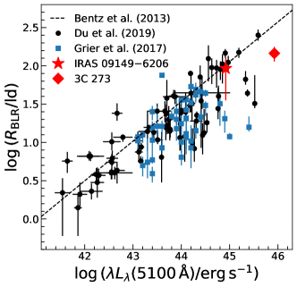
Figure 10: Comparison of the BLR radii for IRAS 09149$-$6206 and 3C 273 measured with GRAVITY to those based on the reverberation mapping time lag. The black circles are the RM measurements collected from the literature by Du & Wang (2019), which mainly include data from Bentz et al. (2013) and the SEAMBH campaign (see text for details). The blue squares are based on H$\beta$ time lags from the SDSS-RM project Grier et al. (2017b). The dashed line is the best-fit radius–luminosity relation from Bentz et al. (2013).

5 Black hole mass and the radius-luminosity relation

One of the parameters in the BLR model is the black hole mass. For the Keplerian model, Table 3 shows that the best fitting value is $1.1\times 10^{8}$ M_⊙. The posterior probability distributions in Fig. 18 show that it is correlated with the mean radius $R_{\rm BLR}$ and the inclination angle $i$, and this is likely what drives the large formal uncertainty of +0.3/$-$0.4 dex. Interestingly, Fig. 20 shows that the correlation is weaker for the outflow model, and that the black hole mass derived is rather similar at $0.5\times 10^{8}$ M_⊙. This is likely because the outflow velocities are linked to the local Keplerian speed in the P14 model. As a result, as noted previously, one should be cautious when interpreting the black hole mass derived from the outflow model.

The only other report of the black hole mass is by Koss et al. (2017) for single-epoch estimates (which can have large uncertainties) based on the broad Balmer lines . Using the method of Trakhtenbrot & Netzer (2012) with the H$\beta$ line, these authors estimate a mass of $3.8\times 10^{8}\,M_{\odot}$. Similarly, using the method of Greene & Ho (2005) for the H$\alpha$ line they find a mass of $2.4\times 10^{8}\,M_{\odot}$. Although slightly less than these, our new value is fully consistent within the uncertainties of the methods used. There is no reported measurement of the stellar velocity dispersion in the literature, making it difficult to place this object on the $M_{\rm BH}$–$\sigma_{*}$ relation. However, as has been commonly done, we can use the width of the [O III] line. From the numbers reported by Perez et al. (1989), we can estimate the dispersion as 250 km s^-1. This puts IRAS 09149$-$6206 only a factor 2–3 below the relation as defined by Gültekin et al. (2009), which is within the scatter. Although the object is a factor 5 below the full relation of McConnell & Ma (2013), this offset is reduced when one considers the relation they find for late-type galaxies. Good agreement is also found if we adopt the correlations for the late-type galaxy sample from Greene et al. (2019). This object therefore does not appear to be unusual in terms of its black hole mass.

We calculated the virial factor, $f_{\mathrm{FWHM}}\equiv GM_{\mathrm{BH}}/(R_{\mathrm{BLR}}v_{\mathrm{FWHM}}^{2})$, by randomly drawing the BLR model parameters from the posterior parameter space sampled from our fitting procedure. The FWHM of the model line profile was used to calculate the velocity, $v_{\mathrm{FWHM}}$. From the Keplerian model, $f_{\mathrm{FWHM}}=0.59^{+0.67}_{-0.26}$, while $f_{\mathrm{FWHM}}=0.31^{+0.25}_{-0.09}$ from the outflow model, again statistically consistent with each other. The typical $f_{\mathrm{FHWM}}$, based on calibration against the $M_{\rm BH}$–$\sigma_{*}$ relation, is $\sim 1.3$ (e.g., Onken et al. 2004; Woo et al. 2010; Ho & Kim 2014). The difference in the virial factor explains most of the difference between our BH mass and those from the single-epoch estimate. Remarkably, Ho & Kim (2014) found $f_{\mathrm{FHWM}}\approx 0.5$ for AGNs with pseudobulges. Unfortunately, high resolution imaging is not available to reveal the bulge properties of IRAS 09149$-$6206. Although the average $f_{\mathrm{FHWM}}$ from BLRs with dynamical modelling is about 1 (Williams et al., 2018), the inferred value of $f_{\mathrm{FHWM}}$ for individual AGNs shows a wide distribution. In particular, the AGNs with similar BLR structure from RM dynamical modelling, Arp 151 (Pancoast et al., 2014b) and Mrk 142 (Li et al., 2018), also show a comparably low $f_{\mathrm{FHWM}}$.

The BLR size of IRAS 09149$-$6206 is robustly measured from our data. In Fig. 10, we compare the BLR radius of IRAS 09149$-$6206 and 3C 273 measured with GRAVITY to the radius–luminosity (R–L) relation of the RM results. Du & Wang (2019) provide the most recent collection of 75 H$\beta$ time lags from various reverberation campaigns during the past two decades. The collection primarily includes 41 AGNs from Bentz et al. (2013) and 25 AGNs with high accretion rate from the SEAMBH campaign (Du et al., 2014, 2015, 2016b, 2018b). We also compare with 44 H$\beta$ time lags from the SDSS-RM campaign (Grier et al., 2017b), which is based on a homogeneously selected quasar sample (Shen et al., 2015). The BLR radius and 5100 Å continuum luminosity of IRAS 09149$-$6206 are 89 light days and $8.32\times 10^{44}\,\mathrm{erg\,s^{-1}}$ (Koss et al., 2017), respectively. Those of 3C 273 are 146 light days (GC18) and $8.43\times 10^{45}\,\mathrm{erg\,s^{-1}}$ (Zhang et al., 2019), respectively. Both IRAS 09149$-$6206 and 3C 273 show good consistency with the RM results. Moreover, IRAS 09149$-$6206 is very close to the best-fit relation from Bentz et al. (2013).

Towards the high luminosity end of the R–L relation, the RM results also show large scatter and tend to drop below the best-fit relation from Bentz et al. (2013), which we refer to as the ‘standard’ R–L relation. A study of high accretion rate AGNs finds a deviation from this relation that is primarily driven by accretion rate (Du et al., 2015; Du & Wang, 2019). These authors proposed that the size of the BLR is reduced at high accretion rate due to the anisotropic emission of the ‘slim’ accretion disk (Abramowicz et al., 1988). Interestingly, the BLR radii measured from the SDSS-RM campaign also lie mostly below the R–L relation, although the accretion rates of these AGNs are not high by the standard of the SEAMBH AGNs (Grier et al., 2017b; Fonseca Alvarez et al., 2019). With the bolometric luminosity $\sim 2\times 10^{45}\,\mathrm{erg\,s^{-1}}$ (GC20a), the Eddington ratio of IRAS 09149$-$6206 is $\sim 0.2$. Following Equation (2) of Du et al. (2015) and adopting $i\approx 21{\mbox{${}^{\circ}$}}$ from our best-fit Keplerian model, the dimensionless accretion rate of IRAS 09149$-$6206 is $\dot{\mathcal{M}}\approx 4.1$. This is about the limit beyond which AGN start to deviate from the R–L relation. With $i\approx 12{\mbox{${}^{\circ}$}}$ (GC18), the dimensionless accretion rate of 3C 273 is $\sim 23.8$. The accretion rate estimates are quantitatively consistent with IRAS 09149$-$6206 being close to the R–L relation, while 3C 273 slightly deviates from it.

In closing, we note that different emission lines may trace regions at different radii of the BLR (e.g., Gaskell & Sparke 1986; Clavel et al. 1991; Peterson et al. 1991; Kaspi et al. 2000; Bentz et al. 2010; Grier et al. 2017b). For example, the H$\alpha$ lag is expected to be larger than the H$\beta$ lag due to radial stratification and optical depth effects (e.g., Rees et al. 1989; Korista & Goad 2000, 2004; Bottorff et al. 2002; Netzer 2020). Zhang et al. (2019) found the H$\beta$ time lag of 3C 273 is fully consistent with the BLR radius measured by GRAVITY from the Pa$\alpha$ emission, after de-trending the contamination from the jet emission (Li et al., 2019). Considering that H$\beta$ and Pa$\alpha$ both come from the $n=4$ level of hydrogen, Wang et al. (2020) argued that the two lines are likely to originate from similar regions of the BLR. They also estimated the possible size difference ($\sim 13\%$) of the H$\beta$ and Pa$\alpha$ emission regions based on the difference of their FWHM. The size difference of H$\beta$ and Br$\gamma$ for IRAS 09149$-$6206 is less clear than that of 3C 273, as the two lines come from different upper levels. However, we find the FWHM of Br$\gamma$ is $\sim 3350\,\mathrm{km\,s^{-1}}$, which is very close to the H$\beta$ FWHM $\sim 3500\,\mathrm{km\,s^{-1}}$ (Perez et al., 1989). Following Wang et al. (2020), we estimate a size difference between the H$\beta$ and Br$\gamma$ emitting regions of $\lesssim 10\%$.

6 Origin of the spatial offset between BLR and continuum photocentre

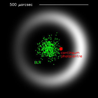
Figure 11: Cartoon illustrating a possible cause for the observed offset between the near-infrared continuum photocentre and the BLR. Dust continuum is assumed to follow a ring that is centred on the BLR and with radius based on the size measurement of GC20a. Brightness variation along this ring causes the offset between BLR and continuum photocentre. Variation in brightness of the hot dust distribution along a ring is supported by the resolved observations of NGC 1068 reported by Gravity Collaboration et al. (2020b).

Our models (Table 3) place the continuum photocentre outside the bulk of the BLR cloud distribution, at a physical scale $\sim 0.14$ pc. While there could be many possible explanations for such an offset, we argue that it is consistent with the simplest explanation: both BLR and dust are centred on the black hole but there is a modest level of asymmetry in the $K$-band emission which is arising from hot dust on scales larger than the BLR, near the sublimation radius. An asymmetry might arise from differential brightness between the near and far sides, from clumpiness or irregularities in the emitting dust structure, or possibly also if the edge of a foreground dust lane crosses the line of sight to the nucleus. The first of these is illustrated in the cartoon of Fig. 11, where, inspired by the asymmetric ring-like dust emission of NGC 1068 (Gravity Collaboration et al., 2020b) we assume a dust ring with radius based on the $K$-band size measurement for IRAS 09149$-$6206 by GC20a. A linear brightness gradient is imposed to reproduce the shift between geometric centre of both BLR and dust ring, and the continuum photocentre. Such asymmetries will lead to nonzero continuum closure phases, but these remain small for compact sources. For the specific configuration of Fig. 11, closure phases $<1$^∘ are expected, consistent with the measurements shown in Fig. 5. More generally, in the marginally resolved limit, the maximum closure phase on VLTI triangles is approximately, $1^{\circ}(\rm FWHM/0.6\rm mas)^{3}$, where the source FWHM is scaled to that measured from FT data for IRAS 09149-6206.

The Fig. 11 scenario is clearly not unique, but one of the simple and plausible ways to create an offset between BLR and continuum photocentre, while staying consistent with all GRAVITY observations. Other plausible ways include a tilted view at non-planar (e.g. bowl-shaped) dust emission. And finally, more exotic explanations for an offset are not ruled out, such as the recoil option discussed in Sec. 4.5.

7 Conclusion

With 7.8 hours on-source integration of GRAVITY, we successfully spatially resolve the broad Br$\gamma$ emission line region of IRAS 09149$-$6206. This is the second source, following 3C 273 (GC18), for which near-infrared interferometric observations directly constrain the size of the BLR and enable an estimate of the mass of the central black hole. With an improved phase calibration method, the differential phase can be uniformly calibrated to systematic uncertainty $\sim 0.05{\mbox{${}^{\circ}$}}$ for each baseline. This enables us to robustly resolve the BLR of the nearby AGN with the broad Br$\gamma$ line. The main results are summarised as follows.

• We obtain a $\sim 0.5{\mbox{${}^{\circ}$}}$ differential phase signal on two baselines, which is measured from the Br$\gamma$ emission line with a peak flux that is $\sim 6\%$ of the continuum. The differential visibility amplitude of the BLR is $\sim 0.8\%$ above the continuum, indicating that the BLR is much more compact than the continuum emission. The closure phase of the continuum emission is $\sim 0{\mbox{${}^{\circ}$}}$, consistent with the continuum being only marginally resolved.

• The model-independent reconstruction of photocentres reveals that the BLR is offset to the east of the photocentre of the continuum by $\sim 120\,\mu$as. While the offset dominates the differential phase signal, the photocentres display a significant blue–red velocity gradient in a north–south direction, indicating that we are resolving the kinematics of broad Br$\gamma$ emission.

• We model the interferometric data with (1) a simplified BLR model including only clouds on circular orbits and (2) a generalised dynamical model that allows for radial motions, and which is widely used in analysing AGN reverberation mapping data. Both models provide an adequate fit to the data. We argue against the outflow model because there are several difficulties associated with its physical interpretation and implication, and caution is needed when interpreting the parameters from the fit. Based on the favoured Keplerian model, and with 95% credibility intervals, we report a radius for the BLR of $65_{-39}^{+30}\,\mu$as or $89_{-53}^{+41}$ light days, and a black hole mass $1.1_{-0.84}^{+1.80}\times 10^{8}\,M_{\odot}$.

• The BLR radii measured by GRAVITY (Br$\gamma$ size for IRAS 09149$-$6206 and Pa$\alpha$ size for 3C 273) are quantitatively consistent with the radius–luminosity relation based on H$\beta$ reverberation mapping of AGNs.

Appendix A Calibration of the pipeline reduced differential phase

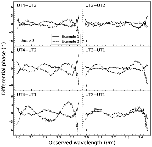
Figure 12: Variation of the differential phase of GRAVITY data. The solid and dashed curves display the differential phases of two observations of calibrator stars, whose differential phase should be consistent with $0{\mbox{${}^{\circ}$}}$. The vertical bar in the lower left corner of each panel indicates the typical uncertainty, enlarged by a factor of three for clarity.

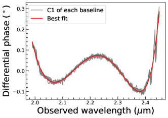
Figure 13: First principle components (C1) from the PCA of all of the baselines (grey curves), before and after the GRAVITY intervention, separately, are very consistent with each other. We fit them together with an 8th order polynomial (red curve). The strong variations beyond 2.4 $\mu$m are due to the resonances of water vapour (Colavita et al. 2004).

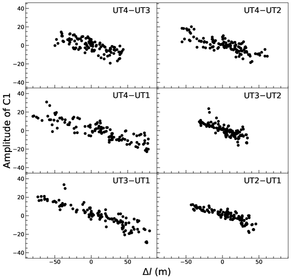
Figure 14: Amplitude of the C1 component as a function of the length difference between the non-vacuum delay lines in each baseline.

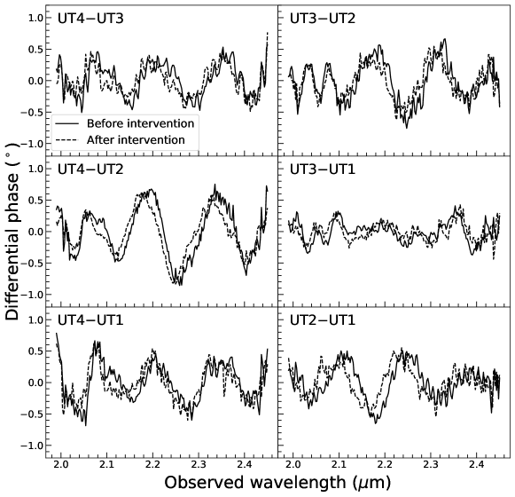
Figure 15: Stable phase features for each baseline, before (solid) and after (dashed) the intervention of GRAVITY.

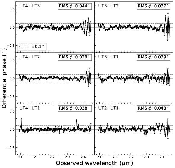
Figure 16: Differential phase of the calibrator stars, flattened and stacked in the same way as the AGN. The 23 calibrator files after the GRAVITY intervention in late 2019 are used, which is quantitatively close to the results using the 122 files before the intervention. The RMS of the phase at 2.05 to 2.40 $\mu$m is reported on the upper right corner of each panel.

As shown in Fig. 12, the pipeline reduced differential phases of the calibrator stars show, at different times, considerable non-zero variation as a function of wavelength. To investigate this, we have collected from the ESO archive on-axis observations of calibrator stars with the same spectral resolution and polarisation configuration. Before the exchange of the GRAVITY science detector during the intervention in October 2019, we found 122 good files. We found 23 good files after the intervention, up to March 2020. The calibrator data reveal a clear systematic phase variation. A principle component analysis (PCA) shows that there is only one variable component dominating the whole variation of the differential phase in all of the baselines. We refer to this variable component as C1 (Fig. 13), which stays the same both before and after the intervention of GRAVITY.

Using PCA, we also find the variability is introduced by the dispersion of the air in the non-vacuum delay line. The amplitude of the C1 component is well correlated with the light path difference in the delay line (Fig. 14). In addition, we also find stable instrumental phase features, that are likely to come from the Fabry-Pérot effect of the elements in the cryostat of GRAVITY. As shown in Fig. 15, these features changed after the GRAVITY intervention, which is expected since the cryostat was opened and many elements were adjusted.

We therefore flatten the pipeline reduced AGN data by fitting and subtracting an instrumental phase model. This includes the stable phase feature as well as the C1 component, the amplitude of which is determined from the fit. The data before and after the intervention are fit separately using the appropriate stable phase feature. We measure the systematic uncertainty of the differential phase after removing the instrumental features using the calibrator data. As Fig. 16 shows, the calibrator differential phases, observed after the intervention, are reduced and stacked in the same way as the AGN data. The stacked differential phases are fully consistent with zero, and have an RMS close to, or better than, 0.05^∘. The phase at $\lesssim 2.05\,{\mbox{$\mu$m}}$ and $\gtrsim 2.40\,{\mbox{$\mu$m}}$ suffers strongly from the absorption bands of carbon dioxide and water in the atmosphere, therefore the phase variation increases at those wavelengths. For calibrator data taken before the intervention, we find the RMS of the stacked differential phases is quantitatively similar to that in Fig. 16. We therefore conclude that the systematic uncertainty of the differential phase is 0.05^∘. We also find that the accuracy of the flattening is insensitive to the choice of the wavelength mask (e.g. across an emission line), as long as the mask is only a reasonable fraction of the entire spectrum. This is because we only have one free parameter in the fit, the amplitude of the C1 component, which has an unvarying profile.

The pipeline uses a 3rd order polynomial to fit the phase of the complex visibility ($R+iI$) of each DIT to derive the self-reference phase ($\phi_{\mathrm{self}}$). The corrected visibility ($R^{\prime}+iI^{\prime}$) of each DIT is,

$$R^{\prime}= \cos(\phi_{\mathrm{self}})R-\sin(\phi_{\mathrm{self}})I,$$

$$I^{\prime}= \sin(\phi_{\mathrm{self}})R+\cos(\phi_{\mathrm{self}})I$$ (13)

It would be very convenient if we could avoid the a posteriori flattening by adopting a better self-reference phase model that takes into account the dispersion of the air. Unfortunately, we find that the models of the refractive index of the air are not accurate enough, in terms of their functional form, for our accuracy requirement (Ciddor 1996). We also tested whether a higher order polynomial fit can remove the effect of the dispersion of the air. However, even fitting with a 7th order polynomial still leaves a residual larger than 0.1^∘, and using such a high order polynomial is risky because it may also fit the scientific phase signal. Therefore, we prefer to apply the separate phase flattening method described above after the default pipeline data reduction.

Appendix B The differential phase of AGN BLRs

In this section, we derive the generalised differential phase of the AGN including the continuum phase, under the assumption that the BLR and continuum are marginally resolved. The complex visibility is defined as,

$$\tilde{V}=V(\lambda)\,e^{i\phi_{\lambda}}=\frac{\iint I_{\lambda}(\@vec{\sigma})\,e^{-2\pi i\,\@vec{u}\cdot\@vec{\sigma}}\,dl\,dm}{\iint I_{\lambda}(\@vec{\sigma})\,dl\,dm},$$ (14)

where $V(\lambda)$ and $\phi_{\lambda}$ denote the visibility amplitude and phase as functions of wavelength ($\lambda$); $I_{\lambda}(\@vec{\sigma})$ is the source intensity distribution; $\@vec{\sigma}=(l,m)$ coordinate on the sky; $\@vec{u}=\@vec{B}/\lambda=(u,v)$ is the baseline vector. When the source is only marginally resolved, i.e., $2\pi\,\@vec{u}\cdot\@vec{\sigma}\ll 1$, we have $e^{-2\pi i\,\@vec{u}\cdot\@vec{\sigma}}\approx 1-2\pi i\,\@vec{u}\cdot\@vec{\sigma}$ and $e^{i\phi_{\lambda}}\approx 1+i\phi_{\lambda}$. Therefore, from equation (14) and setting $V(\lambda)\approx 1$,

$$\phi_{\lambda}\approx-2\pi\,\@vec{u}\cdot\iint I_{\lambda}(\@vec{\sigma})\@vec{\sigma}\,dl\,dm=-2\pi\,\@vec{u}\cdot\@vec{x}_{\lambda},$$ (15)

where $\@vec{x}_{\lambda}$ is defined as the photocentre of the source at the wavelength $\lambda$. The phase is proportional to the photocentre of the source projected onto the baseline. For three baselines that form a closed triangle, i.e., $\@vec{u}_{1}+\@vec{u}_{2}+\@vec{u}_{3}=0$, their closure phase is naturally, $\phi_{1,\lambda}+\phi_{2,\lambda}+\phi_{3,\lambda}=-2\pi\,(\@vec{u}_{1}+\@vec{u}_{2}+\@vec{u}_{3})\cdot\@vec{x}_{\lambda}=0$.

The observed AGN emission consists of two components, the continuum emission from the hot dust and the line emission from the BLR. Therefore, the observed complex visibility is,

$$\tilde{V}=\frac{f_{c,\lambda}\tilde{V}_{c}+f_{\mathrm{BLR},\lambda}\tilde{V}_{\mathrm{BLR}}}{f_{c,\lambda}+f_{\mathrm{BLR},\lambda}},$$ (16)

where $f_{c,\lambda}$ and $\tilde{V}_{c}$ are the spectral flux and complex visibility of the continuum emission as functions of the wavelength, while $f_{\mathrm{BLR},\lambda}$ and $\tilde{V}_{\mathrm{BLR}}$ are the flux and complex visibility of the BLR. Under the marginally resolved assumption, the differential phase is

$$\Delta\phi_{\lambda}=\phi_{\lambda}-\phi_{c}=\frac{f_{\lambda}}{1+f_{\lambda}}\,(\phi_{\mathrm{BLR},\lambda}-\phi_{c}),$$ (17)

where $\phi_{c}$ is the phase of the continuum, which is not expected to vary with different spectral channels; $\phi_{\mathrm{BLR},\lambda}$ is the phase of the BLR as a function of wavelength; and $f_{\lambda}\equiv f_{\mathrm{BLR},\lambda}/f_{c,\lambda}$ is the emission line flux normalised by the continuum. Taking Equation (15) for the continuum and BLR separately into Equation (17), we obtain

$$\Delta\phi_{\lambda}=-2\pi\,\frac{f_{\lambda}}{1+f_{\lambda}}\,\@vec{u}\cdot(\@vec{x}_{\mathrm{BLR,\lambda}}-\@vec{x}_{c}),$$ (18)

where $\@vec{x}_{\mathrm{BLR,\lambda}}$ and $\@vec{x}_{c}$ are the photocentres of the BLR and the continuum.

When we use the BLR model to fit the data, we calculate the differential phase based on Equation (17). The BLR clouds contribute to $\phi_{\mathrm{BLR}}$, while the offset of the BLR contributes to the continuum phase,

$$\Delta\phi_{\lambda}=\frac{f_{\lambda}}{1+f_{\lambda}}\,[\phi_{\mathrm{BLR},\lambda}-2\pi\,(ux_{\mathrm{o}}+vy_{\mathrm{o}})],$$ (19)

where $\{x_{\mathrm{o}},y_{\mathrm{o}}\}$ is the vector of the offset of the BLR with respect to the photocentre of the continuum.

Appendix C Bayesian inference

We infer the optimal model parameters ($\@vec{\Theta}$) based on the interferometric data ($D$) and our prior knowledge of the source and the model ($I$), according to Bayes’ theorem,

$$p(\@vec{\Theta}|D,I)=\frac{p(\@vec{\Theta}|I)p(D|\@vec{\Theta},I)}{p(D|I)},$$ (20)

where $p(\@vec{\Theta}|D,I)$ is the posterior probability density function of the model parameters. The prior, $p(\@vec{\Theta}|I)$, is provided by our prior knowledge about the probability distribution of the model parameters. The evidence, $p(D|I)$, is useful to compare across different models using the Bayes factor,

$$K=\frac{p(D|I_{\mathrm{model\leavevmode\nobreak\ 2}})}{p(D|I_{\mathrm{model\leavevmode\nobreak\ 1}})},$$ (21)

assuming the prior knowledge of model 1 and model 2 are equivalent. The likelihood function, $\mathcal{L}=p(D|\@vec{\Theta},I)$ is defined assuming a Gaussian probability distribution,

$$\ln\,\mathcal{L}=-\frac{1}{2}\sum_{i}^{n}\left(\frac{(f_{i}-\tilde{f}_{i}(\@vec{\Theta}))^{2}}{\sigma_{f,i}^{2}}+\ln\,(2\pi\sigma_{f,i}^{2})\right)$$ (22)

$$-\frac{1}{2}\sum_{i}^{n}\left(\frac{(\phi_{i}-\tilde{\phi}_{i}(\@vec{\Theta}))^{2}}{\sigma_{\phi,i}^{2}}+\ln\,(2\pi\sigma_{\phi,i}^{2})\right)$$ , (23)

where $f_{i}$ and $\sigma_{f,i}$ are the normalised line flux and its uncertainty, respectively, at the $i$th spectral channel; $\phi_{i}$ and $\sigma_{\phi,i}$ are the differential phase and its uncertainty, respectively; and $\tilde{f}_{i}(\@vec{\Theta})$ and $\tilde{\phi}_{i}(\@vec{\Theta})$ are the normalised line flux and differential phase from the BLR model.

We sample the posterior distribution and calculate the Bayesian evidence for each of the two models using the nested sampling method implemented in the Python package, dynesty (Speagle 2020). The nested sampling method has been extensively used for reverberation mapping studies of the BLR (e.g., Pancoast et al. 2014b; Grier et al. 2017a; Li & Wang 2018; Li et al. 2018, 2019; Williams et al. 2018; Raimundo et al. 2019, 2020; Wang et al. 2020), due to its efficiency in sampling the posterior even when there are complex multimodal structures. The best-fit model parameters and the uncertainties (Table 3) are estimated, respectively, from the maximum a posteriori value and the 95% (2 $\sigma$) credible interval of the posterior probability density distributions. The Bayesian evidences are used to compare the probability of the two models with the Bayes’ factor. We also calculate the $\chi_{\mathrm{r}}^{2}$, Bayesian information criterion (BIC, Schwarz 1978), and Akaike information criterion (AIC, Akaike 1973; Hurvich & Tsai 1989),

$$\chi_{\mathrm{r}}^{2} = \Sigma^{N}_{i}\left(\frac{(f_{i}-\tilde{f}_{i}(\@vec{\Theta}))^{2}}{\sigma_{f,i}^{2}}+\frac{(\phi_{i}-\tilde{\phi}_{i}(\@vec{\Theta}))^{2}}{\sigma_{\phi,i}^{2}}\right)\bigg{/}(N-k),$$ (24)

$$\mathrm{BIC} = k\ln\,N-2\ln\,\mathcal{L}_{\mathrm{max}},$$ (25)

$$\mathrm{AIC} = 2k-2\ln\,\mathcal{L}_{\mathrm{max}}+\frac{2k(k+1)}{N-k-1}$$ (26)

where $N$ is the number of data points, $k$ is the number of free parameters, and $\mathcal{L}_{\mathrm{max}}$ is the maximum likelihood based on the samples from the fit.

Appendix D Plots of the BLR model fits and results

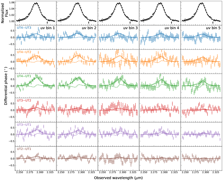
Figure 17: The Keplerian model best-fit spectrum and phases. The first row displays the same normalised spectrum. The black solid line is the best-fit model. The rows are the differential phases of different baselines. Each column displays the phases of each $uv$ bin. In each panel, the solid line is the total phase signal, which sums up the differential phase of the BLR (dashed line) and the continuum phase (dotted line) due to the offset between the BLR and the photocentre of the continuum.

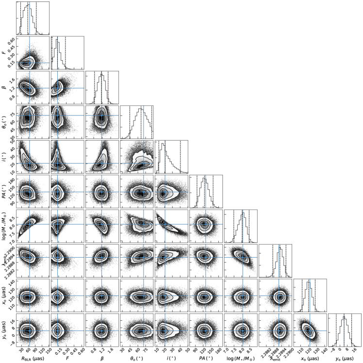
Figure 18: The posterior probability distribution of selected parameters from the Keplerian model. The blue lines and the cross points represent the maximum a posteriori.

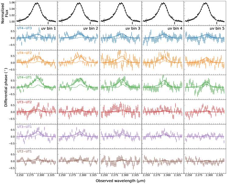
Figure 19: The outflow model best-fit spectrum and phases. The arrangements and symbols are the same as Fig. 17.

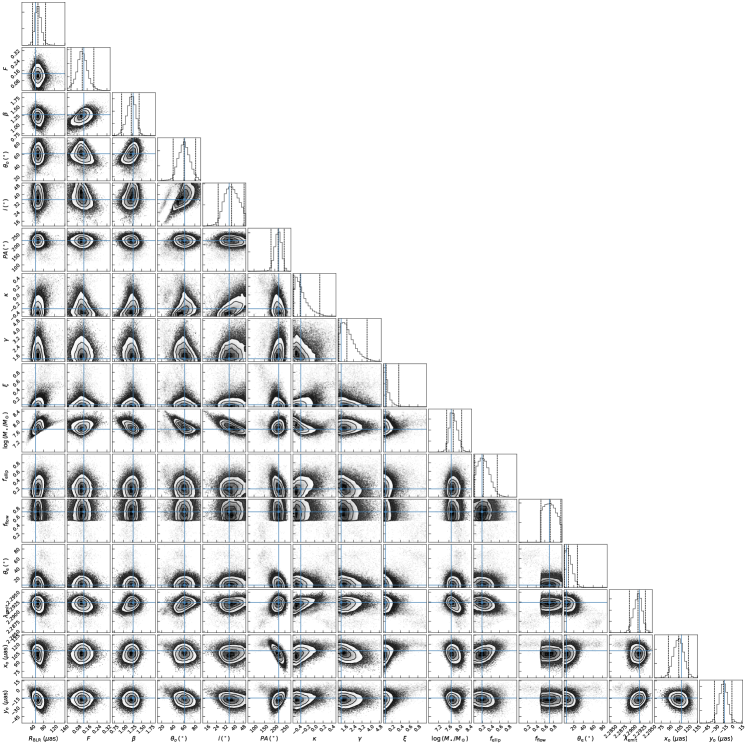
Figure 20: The posterior probability distribution of selected parameters from the outflow model. The blue lines and the cross points represent the maximum a posteriori.

The fits to the flux spectra and the differential phases for each baseline and angular uv bin are displayed in Fig. 17 and Fig. 19 for the Keplerian model and the outflow model respectively. The models were fit to the 5 bins of averaged differential phase based on $uv$ coverage (Fig. 2) in order to minimise smearing and ensuring the signal is still visible. The posterior probability density distributions of the physical parameters that are important for our discussion are plotted in Fig. 18 and Fig. 20.

Appendix E Additional tests of the BLR modelling

In order to reduce the number of parameters, we considered a simplified version of the P14 model in which we fix $\sigma_{\rho,\mathrm{circ}}=\sigma_{\Theta,\mathrm{circ}}=0$, so that bound orbits are always circular, and $\sigma_{\rho,\mathrm{radial}}=\sigma_{\Theta,\mathrm{radial}}=0$ so that orbits with radial motion are always at the same location on the phase space ellipse defined by Equation (6). In addition we set $\sigma_{\mathrm{turb}}=0$ so that there is no additional macroturbulence. The outcome is that the inferred parameters of this simplified model are entirely consistent with the full P14 model. This and further tests suggest that these five technical parameters ($\sigma_{\rho,\mathrm{circ}}$, $\sigma_{\Theta,\mathrm{circ}}$, $\sigma_{\rho,\mathrm{radial}}$, $\sigma_{\Theta,\mathrm{radial}}$, and $\sigma_{\mathrm{turb}}$) are less important in terms of defining the model. This is consistent with the fact that these parameters are largely ignored by Pancoast et al. (2014b) and other works that use the model to fit RM data. In the main text here, we therefore also do not discuss the specific values of these technical parameters.

We interpret the dominant differential phase signal as the continuum phase, which is produced by the offset between the BLR and the photocentre of the continuum emission. However, in Section 4.3 on the outflow model, we show that the BLR alone is also able to produce an asymmetric differential phase with an all positive signal shape. It is therefore interesting to test whether the outflow model is able to fit the data without the need for a continuum phase, so that the BLR would lie at the centre of the continuum emission. We are indeed able to fit the differential phase data reasonably well. However, the inferred radius of the BLR is very large, with $R_{\mathrm{BLR}}\approx 200\,\mu\mathrm{as}$. This is easily understood because the best-fit dynamical model in Section 4.1 has a mean radius $R_{\mathrm{BLR}}\approx 60\,\mu\mathrm{as}$, which corresponds to a phase signal $\sim 0.15{\mbox{${}^{\circ}$}}$ shown in Fig. 8 (b). When the continuum phase is fixed to be zero, the BLR size has to increase by a factor of $\sim 3$ in order to fit the much larger $\sim 0.5{\mbox{${}^{\circ}$}}$ phase signal. However, in GC20a we found that the size of the continuum emission for IRAS 09149$-$6206, measured as a Gaussian FWHM, is only 0.54–0.64 mas. Thus its BLR radius should be $<100$ $\mu$as, since it must be significantly smaller than the continuum. Similarly, following the method presented in Sec. 4.4, we find the differential visibility amplitude of the large BLR model to be about a factor 2 lower than the other two models shown in Fig. 4. Therefore, the differential visibility amplitude data strongly disfavour the large BLR model.

We also attempted to include the differential visibility amplitude data in the fit. However, as the differential visibility amplitude is very sensitive to the relative size between BLR and the continuum, the inferred BLR size strongly depends on the assumed FWHM of the continuum emission. Using $\mathrm{FWHM}=0.6$ mas, our inferred BLR sizes are only $21_{-9}^{+22}$ and $30_{-18}^{+24}$ $\mu$as for the Keplerian and outflow models respectively. GC20a estimated the FWHM of the continuum emission to be $0.54\pm 0.05$ mas by directly fitting the visibility amplitude of the fringe tracker data (the ‘FT size’ in their Table 2). From the differential visibility amplitude of the science channel, they also obtained a size of $0.64\pm 0.06$ $\mu$as (the ‘SC size’). Under the marginally resolved limit, the latter method only yields the correct continuum size when the BLR is exactly a point source; for better resolved sources, the derived quantity is the quadrature difference between the continuum emission size and the BLR size (Waisberg et al. 2017). Therefore, we should expect the SC size to be slightly smaller than the FT size. This is true for 3C 273 and PDS 456 but not for IRAS 09149$-$6206. Although the problem can be easily explained by the uncertainty, this indicates that the continuum size of IRAS 09149$-$6206 is still quite uncertain. Therefore, we exclude the differential visibility amplitude data from our primary BLR fittings and use it only as a consistency check.

For our last test, we check whether the input parameters can be recovered by fitting mock data generated by the Keplerian model (mock 1) and the outflow model (mock 2). We also test whether the Bayes factor, BIC, and AIC provide a reliable judgement on the model fits. We use the best-fit parameters of the Keplerian model and the outflow model to generate mock data, adopting Gaussian noise based on the measured uncertainty. In the next step, we fit both sets of mock data with both the Keplerian model and the full P14 model. The input parameters are usually recovered if the same model is used to generate and to fit the mock data. Focusing on the mock 2 data, the best-fit Keplerian model results are similar to those in Fig. 17 and Fig. 7. The averaged phase, after subtracting the best-fit continuum phase, still shows clear S-shape profiles. To compare the two models fitting the mock 2 data, the Bayes factor and AIC prefer the P14 model, while the BIC incorrectly selects the Keplerian model. For the fits to mock 1 data, the P14 model can naturally fit the data and provide the parameters consistent with the input, which is as expected. The Bayes factor determines the Keplerian model and the outflow model are equivalent. The AIC incorrectly prefers the outflow model, while the BIC prefers the Keplerian model. In a nutshell, these tests demonstrate that: (1) our models infer the parameters self-consistently when the mock data are generated from them and (2) The Bayes factor provides a reasonable judgement on the preferred model.