Abstract. The COVID-19 pandemic so far has caused huge negative impacts on different areas all over the world, and the United States (US) is one of the most affected countries. In this paper, we use methods from the functional data analysis to look into the COVID-19 data in the US. We explore the modes of variation of the data through a functional principal component analysis (FPCA), and study the canonical correlation between confirmed and death cases. In addition, we run a cluster analysis at the state level so as to investigate the relation between geographical locations and the clustering structure. Lastly, we consider a functional time series model fitted to the cumulative confirmed cases in the US, and make forecasts based on the dynamic FPCA. Both point and interval forecasts are provided, and the methods for assessing the accuracy of the forecasts are also included.

AMS subject classifications.

Primary: 62R10; 62M10

Secondary: 62H30

Key words. COVID-19; canonical correlation; cluster analysis; functional time series; forecasting; principal component analysis

1. Introduction

Ever since December 2019 when the outbreak of the Coronavirus Disease (COVID-19) has first come to the attention of the general public in China, this epidemic has been spread to more than 180 countries over the world, leading to extremely negative impacts on global public health and economy. As of 08/25/2020, this virulent disease has caused a total of 23,721,008 confirmed and 815,029 death cases around the world, according to the data collected at Johns Hopkins University [38]. The United States (US) is the most severely hit country with 5,759,147 confirmed and 177,873 death cases. According to the US Bureau of Labor Statistics, the unemployment rate of US has reached 14.7% in April 2020, a record-high over-the-month increase since January, 1948. Although the rate has declined to 8.4% in August 2020, it still remains at a relatively high level, compared to less than 4% before the pandemic.

A great amount of scientific efforts have been integrated to learn the progression of the disease, and to mitigate its negative impact on people’s normal life. However, according to some recent research [20], it is evident that the COVID-19 has become mutating. As pointed out by Dr. Anthony Fauci, the director of the National Institute of Allergy and Infectious Diseases, on 06/24/2020, the vaccine for the COVID-19 would not likely to be available until 2021. On 07/27/2020, the National Institutes of Health has announced the phase 3 clinical trial of the investigational vaccine for the COVID-19. As currently there is no medication that can directly eliminate the virus, many infected patients have to rely on their own immune systems to recover under the help of standard treatments. As more and more COVID-19 data become available, statisticians now commit to carrying out intensive data-driven analyses to precisely uncover the epidemic characteristics of the COVID-19.

In this paper, we exploit methods from the functional data analysis to analyze the COVID-19 data of both confirmed and death cases in the US from 01/21/2020 to 08/15/2020. In this study, our data are collected at state level (see Section 2 for details), with the following research questions in mind:

• Does the practice of public health measures (e.g., social distancing and mask wearing) help to mitigate the spread of the COVID-19? On the other hand, does the reopening of business exacerbate the spread of the disease?

• Is there any quantitative way to understand the correlation between infections and deaths caused by the COVID-19 in the US? Does the correlation vary from state to state?

• Is the spread of the COVID-19 related to the geographical locations of the infected regions or hot spots (at the state level) in the US?

• Is there a way to have some reasonable forecasts with regard to the total number of confirmed cases nationwide?

2. Preliminary analysis

We collect the number of confirmed and death cases of the COVID-19 from the 50 continental states in the US between 01/21/2020 (the date of the first domestic confirmed case reported in the US) to 08/15/2020 (the weekend before school reopening in most of the states). The data of cumulative confirmed and death cases were collected at state level, from a publicly available repository released and updated by New York Times (https://github.com/nytimes/covid-19-data). In what follows, the daily confirmed and death cases are obtained effortlessly.

The majority of our analyses is done at the state level. Noticing the significant differences in the population size for each state, we standardize the data, using the estimated population size for each state at the end of year 2019 from the US Census Bureau (https://www.census.gov/popclock) to scale all collected data (cumulative and daily cases), and save them in units of “per million”. In Figure 1, we plot the number of daily confirmed and death cases in the US. From early May to early June, the cumulative case-to-fatality rate (CFR) of the COVID-19 in the US has stayed consistently high around 6.01%, close to the estimate (6.1%) given in [1], which is slightly higher than the CFR in Wuhan, China (5.8%) reported on 02/01/2020 [52], and significantly higher than the global CFR (3.4%) according to WHO Director-General’s opening remarks at the media briefing on 03/03/2020. In August, the CFR in the US has declined to 3.1%.

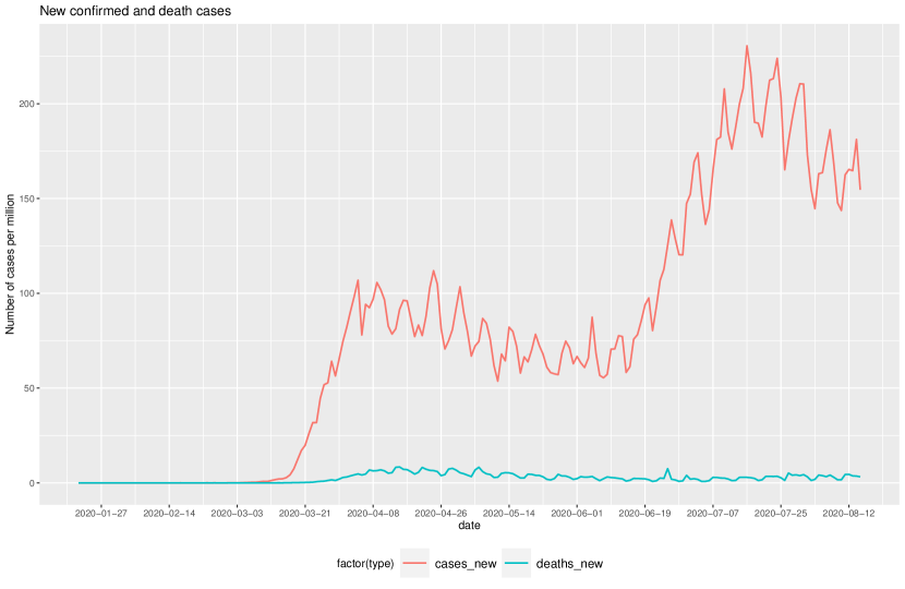
Figure 1. The number of daily confirmed and death cases (per million) in the US from 01/21/2020 to 08/15/2020.

One important epidemic metric for the study of the infectious disease dynamics is the basic reproduction number, usually denoted as $R_{0}$. It refers to the average number of secondary cases per infectious case in a population where all the individuals thereof are susceptible to the infection. A variant called the instantaneous reproduction number, denoted as $R_{t}$, is the average number of cases generated by each infection at a given time $t$. We observe that 33 of 50 continental states in the US has had $R_{t}>1$ (https://rt.live) on 05/29/2020, suggesting that the epidemic has not yet been fully contained by the end of May, 2020. In fact, this proportion climbs to 41 out of 50 in the following month. Upon the end of the study period, the proportion of the states with $R_{t}>1$ has dropped to 16 out of 50, but the whole nation is still faced with the potential risk of a massive spread owing to the reopening of schools in the fall. Some other results of critical epidemic characteristics and dynamics of the COVID-19 in the US have been reported in [54].

In this study, we treat the collected data as functional data, and adopt methods from the functional data analysis (FDA). Figure 2 shows the functional data of daily confirmed and death cases (per million) of the top five states in the US during the study period. As discussed in [58], the FDA methods are applicable to sparsely and irregularly spaced data in time, so are preferred to the standard time series methods in the analyses of the time series data. Besides, the FDA methods manage to capture the functional behavior of the underlying data which generate the process (see [57, 58, 59] for details), and have been widely adopted in a plethora of applications in public health and biomedical studies [70]. In the next few sections, we list the adopted FDA methods, and present the analysis results when they are applied to the COVID-19 data in the US.

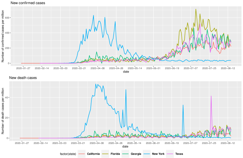
Figure 2. The number of daily confirmed and death cases (per million) of top five continental states in the US.

3. Functional principal component analysis and modes of variation

In multivariate statistics, modes of variation are a set of centered vectors describing the variation in a population or sample. Typically, variation patterns are characterized via the standard eigenanalysis, i.e., principal component analysis [37]. Analogously in the FDA, modes of variation provide an efficient tool to visualize the variation of the functional curves around the mean function. Identifying modes of variation in functional data is usually done through the functional principal component analysis [14], providing new insights and precise interpretations of the functional data.

3.1. Functional principal component analysis

Consider a probability space $(\mathbb{R}_{+},\mathcal{F},{\rm\bf P})$, and a compact interval $I\subset\mathbb{R}_{+}$. A stochastic process $X(\cdot)$ is called an $L_{2}$ process on $I$ if

$${\rm\bf E}\int_{I}|X(t)|^{2}\,dt<\infty.$$

Let $X_{i}$, for $i=1,2,\ldots,n$, be independent realizations of the underlying $L_{2}$ process $X(\cdot)$. By convention in the FDA, functional data are given as

$$Y_{i}(t)=X_{i}(t)+\varepsilon_{i}(t),$$ (1)

for $t\in\mathcal{T}_{i}:=\{t_{ij},j=1,2,\ldots,n_{i}\}$, a time schedule for subject $i$. The terms $\varepsilon_{i}(t_{ij})$’s are independent measurement errors with ${\rm\bf E}(\varepsilon_{i}(t_{ij}))=0$ and ${\rm{\bf V}ar}(\varepsilon_{i}(t_{ij}))=\sigma_{ij}^{2}$ for some constant $\sigma_{ij}$.

The functional principal component analysis (FPCA) is a powerful tool for dimension reduction in the FDA [14]. In essence, FPCA is an expansion of the realization $X_{i}(t)$ into functional bases consisting of the eigenfunctions of the variance-covariance structure of the process $X(\cdot)$, where the eigenfunctions are required to be orthogonal. Let $\{\phi_{k}:k\geq 1\}$ denotes the collection of orthogonal eigenfunctions. In addition, let $\mu(t)={\rm\bf E}(X(t))$ be the true mean function, and $\xi_{ik}:=\int_{I}(X_{i}(t)-\mu(t))\phi_{k}(t)\,dt$ be the $k$-th functional principal component (FPC) of $X_{i}$ (also called scores in the jargon). By the Karhunen–Loève Theorem [40, 48], we have

$$X_{i}(t)=\mu(t)+\sum_{k=1}^{\infty}\xi_{ik}\phi_{k}(t).$$ (2)

Due to the difficulties in estimating and interpreting the infinite sum in Equation (2), a conventional treatment is to approximate it by a finite sum of $K$ terms. In what follows, we set

$$Y_{i}(t)=\mu(t)+\sum_{k=1}^{K}\xi_{ik}\phi_{k}(t)+\upsilon_{i}(t),$$

where $\upsilon_{i}(t)$ is the counterpart of $\varepsilon_{i}(t)$ in Equation (1) owing to truncation. We refer interested readers to [64] for a comprehensive review of the fundamental theory of FPCA. One primary application of FPCA is to explore modes of variation [39] for the functional data, reflecting the percentage of total variations contributed by each principal eigenfunctions.

When applying the FPCA method to the COVID-19 data of the 50 continental states in the US, we notice that they are not identical in time schedules. The identification of the first COVID-19 case may differ by as long as 30 days across the country. Having observed the sparsity in the functional data during the early stage of the outbreak, we adopt the Principal Components Analysis through Conditional Expectation (PACE) approach proposed in [73] for our analysis. The estimation of the FPC score of $\bm{Y}_{i}=(Y_{i}(t_{i1}),\ldots,Y_{i}(t_{in_{i}}))^{\sf T}$, for $i=1,2,\ldots n$, via PACE takes the following major steps:

• For each $\bm{Y}_{i}$, estimate the mean function $\bm{\mu}_{i}=(\mu(t_{i1}),\ldots,\mu(t_{in_{i}}))^{\sf T}$ and the covariance structure $\bm{\Sigma}_{\bm{Y}_{i}}={\rm{\bf C}ov}(\bm{Y}_{i},\bm{Y}_{i})$ by locally linear scatter and surface smoothers, respectively [16];

• Discretize the off-diagonal smoothed covariance to estimate the eigenfunctions $\bm{\phi}_{ik}=(\phi_{k}(t_{i1}),\ldots,\phi_{k}(t_{in_{i}}))^{\sf Tc}$, $k=1,2,\ldots K$, and the corresponding eigenvalue $\lambda_{k}$ [6];

• Adopt an Akaike Information Criterion (AIC) type criterion to select the number of eigenfunctions, i.e., $K$, needed to approximate the process [62];

• Lastly, the estimation of the FPC score for the $i$-th subject is given through the conditional expectation:

  $$\hat{\xi}_{ik}={\rm\bf E}(\xi_{ik}\,|\,\bm{Y}_{i})=\hat{\lambda}_{k}\hat{\bm{\phi}}^{\sf T}_{ik}\hat{\bm{\Sigma}}^{-1}_{\bm{Y}_{i}}(\bm{Y}_{i}-\hat{\bm{\mu}}_{i}),$$ (3)

  where $\hat{\lambda}_{k}$, $\hat{\bm{\phi}}_{ik}$, $\hat{\bm{\Sigma}}_{\bm{Y}_{i}}$ and $\hat{\bm{\mu}}_{i}$ are respectively the estimates of $\lambda_{k}$, $\bm{\phi}_{ik}$, $\bm{\Sigma}_{\bm{Y}_{i}}$ and $\bm{\mu}_{i}$.

In practice, the R package fdapace [7] allows us to apply the PACE method to the functional COVID-19 data directly. The computation results and corresponding discussions are given in the subsequent section.

3.2. Modes of variation

To begin with, we plot the fitted mean curve (which estimates the trend over time), the fitted variance curve (which estimates the subject-specific variation) and the fitted covariance surface of daily confirmed cases across 50 continental states in Figure 3.

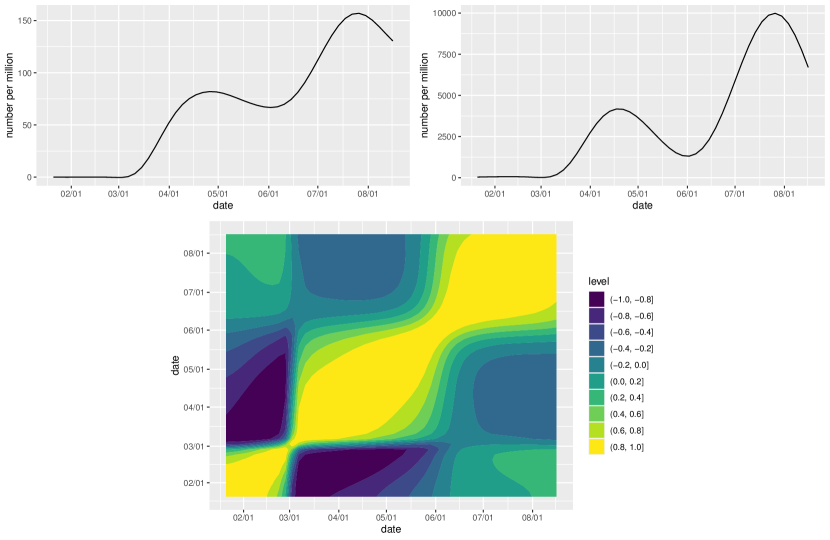
Figure 3. Fitted mean curve (top left panel), fitted variance curve (top right panel) and fitted correlation surface (bottom) of daily confirmed cases of COVID-19 in the US.

The estimated mean is close to $0$ in January and February, and starts climbing since early March until reaches a local maximum in late April. The overall trend in May is downwards, followed by a second wave that starts from June. The curve hits the peak at the end of the third week of July. The estimated variance curve looks similar to the fitted mean curve in shape, which stays low at the very early stage, and deviates from $0$ at the end of the first week of March. The first local maximum emerges around 04/17/2020, and then starts decreasing until 06/01/2020. The global maximum of the curve is observed in the third week of July, corresponding to the worst period of the attack of the COVID-19 to the country. The correlation surface is presented through a contour plot. Measurements at close time points appears to be highly correlated. The correlation between early and very late times are close to $0$, whereas that between early and middle times tends to be negative. The correlation patterns among middle and later times are slightly negative. In particular, the correlation surface reveals that the increase in the number of confirmed cases follows three different stages, where the two break points are respectively 03/01 and 06/01. The strong positive correlation seems more persistent in the latter two stages.

Next we apply the PACE method to the COVID-19 data of daily confirmed cases in the US. The adaptive algorithm selects a total of six eigenfunctions (accounting for more than 99.99% of the total variation), where the first two together explains about 95% of the total variation of the data (see Figure 4), indicating the remaining eigenfunctions are less important.

The first eigenfunction (accounting for 68.38% of the total variation) remains constant close to $0$ during the first month of the study period, and starts decreasing afterwards. The value of the eigenfunction falls negative since 03/01/2020 until it reaches a local minimum around 04/17/2020. After that, the function value keeps increasing until it hits the peak around 07/23/2020. The first eigenfunction defines the most important mode of variation, suggesting that the state-specific intercept term captures the vertical shift (especially later times) in the overall mean. Besides, the first eigenfunction reflects a contrast between middle and late times, where the break point emerges about one week after the announcement of business reopening in the majority of the states in the US.

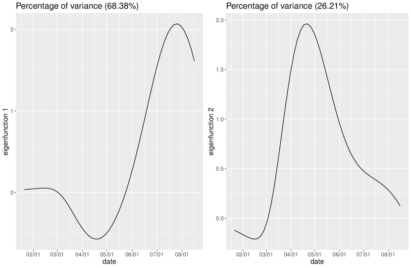
Figure 4. First two eigenfunctions for the US COVID-19 confirmed cases

The second eigenfunction presents a variation around a piecewise linear time trend. The value of the eigenfunction is negative at early times, and becomes positive since March, and hits a break point in the third week of April. Since then, it begins to decrease but stays positive during the rest of the study period. The second eigenfunction suggests that the second largest variation among the states is a scale difference along the direction of this functional curve.

4. Functional canonical correlations

In statistics, canonical correlation analysis is a tool to make inference based on the cross-covariance matrix of multiple datasets. The analogue in FDA, named functional canonical correlation analysis (FCCA), aims to investigate the correlation shared by multiple functional datasets [44]. Specifically, here we use the FCCA method to quantitatively estimate the correlation between confirmed and death cases across the states.

4.1. Functional canonical correlation analysis

We first outline the theoretical setup of the analysis method [22, 23], and refer the interested readers to [71] for a concise review. Let $X(\cdot)$ and $Y(\cdot)$ be two $L_{2}$ processes on two compact intervals, $I_{X}$ and $I_{Y}$, respectively. In addition, let $\mathcal{H}_{2}(I)$ denote the Hilbert space of square-integrable functions on some compact interval $I$, with respect to Lebesgue measure. In addition, the notation $\langle\cdot,\cdot\rangle$ refers to the standard operation of inner product. By definition, the first canonical correlation is given by

$$\rho_{1}=\sup_{u\in\mathcal{H}_{2}(I_{X}),v\in\mathcal{H}_{2}(I_{Y})}{\rm{\bf C}ov}\bigl{(}\langle u,X\rangle,\langle v,Y\rangle\bigr{)}={\rm{\bf C}ov}\bigl{(}\langle u_{1},X\rangle,\langle v_{1},Y\rangle\bigr{)},$$

subject to

$${\rm{\bf V}ar}\bigl{(}\langle u,X\rangle\bigr{)}=1\qquad\mbox{and}\qquad{\rm{\bf V}ar}\bigl{(}\langle v,Y\rangle\bigr{)}=1.$$ (4)

The pair of the optimal solutions $(u_{1},v_{1})$ are called the canonical weight functions of $\rho_{1}$. For $k\geq 2$, the $k$-th canonical correlation coefficient, denoted $\rho_{k}$, is defined under the condition of orthogonality:

$${\rm{\bf C}ov}\bigl{(}\langle u_{k},X\rangle,\langle u_{j},X\rangle\bigr{)}={\rm{\bf C}ov}\bigl{(}\langle v_{k},Y\rangle,\langle v_{j},Y\rangle\bigr{)}=0,\qquad j=1,2,\ldots,k-1.$$

Set $\rho_{k}$, $k\geq 2$, and its associated weight functions $(u_{k},v_{k})$ in an analogous way:

$$\rho_{k}=\sup_{u\in\mathcal{H}_{2}(I_{X}),v\in\mathcal{H}_{2}(I_{Y})}{\rm{\bf C}ov}\bigl{(}\langle u,X\rangle,\langle v,Y\rangle\bigr{)}={\rm{\bf C}ov}\bigl{(}\langle u_{k},X\rangle,\langle v_{k},Y\rangle\bigr{)},$$

subject to condition (4). In FDA, the inner products $\langle u,X\rangle$ and $\langle v,Y\rangle$ corresponding to weight functions $u$ and $v$ are called probe scores. Typically for $k\geq 1$, we refer to $(u_{k},v_{k})$ as the canonical weight pair that optimizes the canonical criteria for $\rho_{k}$.

The FCCA approach, in essence, determines the projection of $X$ in the direction of $u_{k}$ as well as that of $Y$ in the direction of $v_{k}$, such that their linear combinations are maximized for $k\geq 1$. Consider three kinds of variance and cross-covariance operators $\Sigma_{XX}:\mathcal{H}_{2}(X)\mapsto\mathcal{H}_{2}(X)$, $\Sigma_{YY}:\mathcal{H}_{2}(Y)\mapsto\mathcal{H}_{2}(Y)$ and $\Sigma_{YX}:\mathcal{H}_{2}(Y)\mapsto\mathcal{H}_{2}(X)$, which correspond to the variance structure of $X$, the variance structure of $Y$ and the cross-covariance structure between $X$ and $Y$, respectively. We then rewrite the definition expression of $\rho_{1}$ as follows:

$$\rho_{1}=\sup_{u\in\mathcal{H}_{2}(I_{X}),v\in\mathcal{H}_{2}(I_{Y})}\langle u,\Sigma_{YX}\,v\rangle,$$ (5)

subject to $u^{\top}\Sigma_{XX}u=v^{\top}\Sigma_{YY}v=1$. Similar arguments can also be applied to $\rho_{k},k\geq 2$, by accounting for the condition of orthogonality. A standard procedure for the change of basis in Equation (5) implies that the problem is equivalent to an eigenanalysis of $\Sigma_{XX}^{-1/2}\Sigma_{YX}\Sigma_{YY}^{-1/2}$, i.e., a maximization problem of Rayleigh quotient.

In this study, we use functions from the R package fda [60] to implement the FCCA method based on an integration of an exceedingly greedy procedure and an expansion of the functional basis. A variety of methods solving the optimization problem of functional canonical correlations have been developed in the literature; see for example, [59, 22, 23, 72].

Prior to estimating the functional canonical correlation between confirmed cases and death tolls in the US, some additional pre-processing procedures to the data are necessary, as we observe that the date on which the first confirmed case is reported varies significantly across the states, and the number of death counts stays relatively low during the entire study period in several states.

4.2. Canonical correlations between confirmed and death cases

Now we inspect the functional canonical correlation between confirmed and death cases from the 50 continental states in the US. The first step is to pre-process the data. Noticing that diagnostic tests (e.g., swab test) of the COVID-19 have not been widely implemented in most states until late March (for instance, the first drive-through COVID-19 testing site in Philadelphia was not open to the public until 03/20/2020), we reschedule the starting date of study period to 04/01/2020 for the rest of the study in this section. Besides, the cumulative number of (scaled) confirmed and death cases (instead of scaled daily numbers) are used for the analysis so that no state is excluded due to sparsity, especially for those with few cases reported during April and early May.

In the literature, there are several different options of basis functions for the basis expansion in the FCCA. Having observed some periodic features in our functional data, we choose the Fourier basis here. The first canonical correlation is $0.985$, which reveals a dominant pair of modes of variation that are highly positively correlated. The corresponding canonical weight functions are plotted in Figure 5. The canonical weight function of confirmed cases resembles a sinusoidal function with a period of one month approximately, while the counterpart of death cases seemingly contrasts early and middle times to late times (primarily in July). A state has a negative score with a large absolute value on the canonical weight of confirmed cases if it has a large number of confirmed cases in April, late May and early June, but small counts in July and early August. Also, a state has a high positive score on the canonical weight of death cases if it has more death cases in July than any other time during the study period.

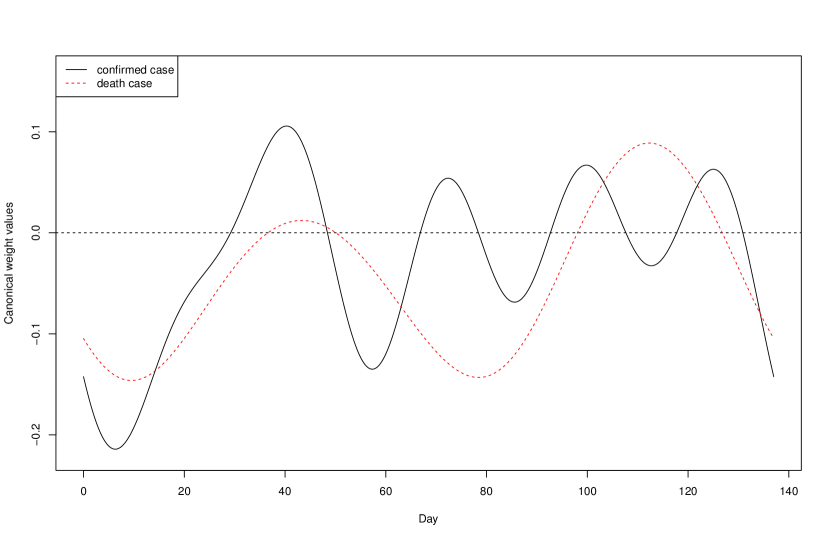
Figure 5. The first pair of canonical weight functions correlating confirmed and death cases of the 50 continental states in the US.

Next we plot the canonical variable scores for the death cases against confirmed cases in Figure 6, where we see that the New York state lies on the bottom left corner. This is due to the fact that the New York state (especially New York City) has a lot of confirmed and death cases at the early stage of the pandemic, but later the transmission of the virus has been well controlled since July, thanks to the complete shutdown of the city as well as the rigorous adherence to public health measures, e.g. the practice of social distancing, mask wearing and the limit of the number of people allowed in essential businesses. Since July, less than 20 deaths has been reported daily in New York City, in contrast with an average of more than 700 deaths every day in April. Therefore, both canonical variable scores remain low in the state of New York.

Another “outlier” is New Jersey, which is geographically adjacent to New York state. The overall trends of confirmed and death cases in New Jersey are similar in shape to those in New York, but both are smaller in magnitude. Therefore, New Jersey sits close to New York in Figure 6. Three states in the middle with negative scores in both canonical variables are Massachusetts, Connecticut and Rhode Island, all of which are geographically close to New York.

All other states are mostly scattered on the top right corner in Figure 6. The one sits at the most top right is Texas, with positive scores in both canonical variables. The confirmed and death cases in Texas are not the largest in the first wave of outbreak (i.e., April and May), but the state has seen a large surge in the daily confirmed and death cases since late June. Consequently, both of the canonical scores of Texas remain positive. In fact, Texas has controlled the spread of the disease well in April when a 14-day self-quarantine has been mandated, all nonessential businesses are closed, and ordered travel restrictions have been instituted between Texas and Louisiana (an outbreak occurs in New Orleans during that period). However, with the stay-at-home order lapsed in May, and the reopening of the economy started in June, Texas has experienced a huge increase in the COVID-19 cases, due to the increasing frequencies of indoor and outdoor gatherings in large groups of people without proper public health measures implemented.

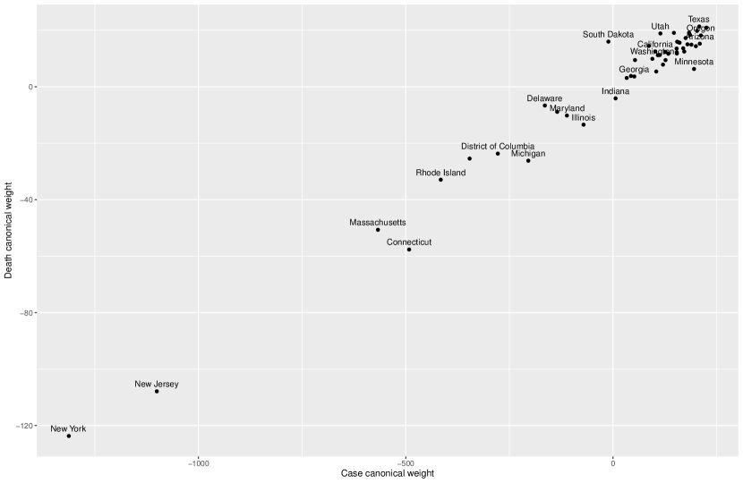
Figure 6. Canonical variable scores of death cases against confirmed cases of the 50 continental states in the US.

5. Functional cluster analysis

Clustering is another common tool for data exploration in multivariate statistics, aiming at constructing homogeneous groups (called clusters) consisting of observed data that present some similar characteristics or patterns [41]. In contrast, observations from different groups are expected to be as dissimilar as possible. The functional cluster analysis (FCA) is an unsupervised learning process for functional data. In this section, we investigate the cluster structure in the US based on cumulative confirmed cases (after being scaled) across the states.

5.1. Methods for functional cluster analysis

Two classical methods for the FCA are hierarchical clustering [17] and $k$-means clustering [2]. More recently, many clustering methods extended from them were proposed. See [35] for a summary.

Traditional $k$-means clustering methods for the FCA, e.g. [2], require a finite set of pre-specified basis functions in order to span a functional space, and assume the observed functional data to admit the basis expansion. The FCA is then completed by applying the standard $k$-means algorithm to the estimated basis coefficients. Alternatively, one may replace basis coefficients with FPC scores (i.e., $\xi_{ik}$’s in Equation (3)) for conducting the cluster analysis [10, 11, 55].

In modern FDA, there are two methods that are extensively popular to conduct the FCA. One approach is the EM-based algorithm [9], which assumes a finite (say $K\in\mathbb{N}$) mixture of Gaussian distributions. The model is given by

$$f(\bm{x}\,|\,\bm{\theta})=\sum_{c=1}^{K}\pi_{c}\psi(\bm{x}\,|\,\bm{\mu}_{c},\bm{\Sigma}_{c}),$$ (6)

where $\bm{\theta}=\{\pi_{1},\ldots,\pi_{K},\bm{\mu}_{1},\ldots,\bm{\mu}_{K},\bm{\Sigma}_{1},\ldots,\bm{\Sigma}_{K}\}$ is a collection of parameters; for each $c=1,2,\ldots,K$, $\pi_{c}\in(0,1)$ is the mixing proportion such that $\sum_{c=1}^{K}\pi_{c}=1$, and $\psi(\bm{x}\,|\,\bm{\mu}_{c},\bm{\Sigma}_{c})$ is a Gaussian distribution with mean $\bm{\mu}_{c}$ and variance $\bm{\Sigma}_{c}$. The log-likelihood of the model in Equation (6) is optimized by the EM algorithm [15]. The setups of the E-step and the M-step are standard, available in a variety of articles, texts and tutorials, e.g. [43]. Given the number of clusters $K$, the EM algorithm partitions a set of $n$ observations $\bm{X}=\{\bm{x}_{1},\ldots,\bm{x}_{n}\}$ into $K$ clusters by maximizing the following expression:

$$\underset{c}{\rm arg\,max}\;\hat{\pi}_{c}\phi(\bm{x}_{i}\,|\,\hat{\bm{\mu}}_{c},\hat{\bm{\Sigma}}_{c})$$

for each $i=1,2,\ldots,n$.

The alternative is the $k$-centers functional clustering (kCFC) algorithm proposed by [10], using the subspace spanned by the FPCs as cluster centers. This approach is popular as the distributional assumptions are relaxed.

Nonetheless, there are limitations in both algorithms. The kCFC algorithm assumes equal within-cluster variance, whereas the EM algorithm assumes a mixture of Gaussian distributions. Relevant discussions on the difference between the two algorithms are included in [35]. In the present analysis, it seems inappropriate to assume equal within-cluster variance, so we adopt the model-based EM algorithm, which is available in R package EMCluster [9]. Since the method is based on the EM algorithm, it is critical to select the initial values of the parameters appropriately. Specifically, we adopt a strategy developed in [5] for the initialization of the algorithm, with corresponding functions available in EMCluster.

5.2. Cluster analysis results

Similar to the FCCA part, we trim the study period to “04/01/2020 to 08/15/2020” as few (or even no) confirmed case has been observed in many states before April. The implementation of the EMCluster algorithm requires the predetermination of the number of clusters in prior. There are a couple of standard methods to obtain an optimal value of $K$. We select the value of $K$ via the elbow method based on the sum of squares of the within-cluster variations. The computation reveals that the most appropriate value of $K$ is $5$, and the optimal clustering strategy associated with $K=5$ is given in Figure 7.

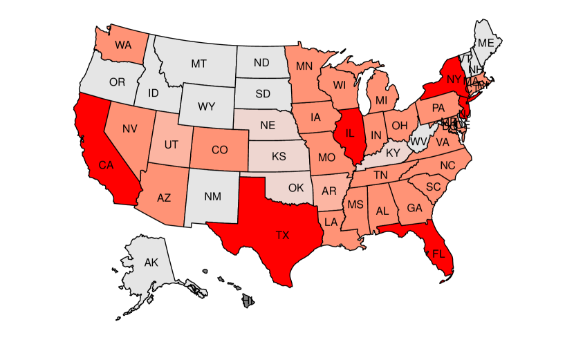
Figure 7. Clustering results based on the number of cumulative confirmed cases in 50 continental states in the US from 04/01/2020 to 08/15/2020.

The first cluster includes New York, New Jersey and Illinois, the three states that have been most severely attacked by the COVID-19 in the first wave, as well as Florida, Texas and California, all of which have experienced a huge surge in both confirmed and death cases in the second wave. Overall, these six states are the worst hit by the COVID-19 throughout the study period.

The second cluster contains 24 states, including Georgia, North Carolina, Massachusetts, Pennsylvania and Washington, etc., most of which are geographically close (but not necessarily adjacent) to the hot-spot regions. Some states, e.g. Georgia, North Carolina and Colorado, actually have reached the peak of the COVID-19 cases in the second wave after the reopening of the business, when some mandatory protocols have been called off. Besides, with the relaxation of travel restrictions, an increase in population movements may also cause the cross infections among the residents in these states. The state of Washington, located at the northwest corner, also belongs to this cluster, where the first case in the US has been reported.

The third cluster only has two states: Utah and Arkansas. Utah is not directly adjacent those epidemic centers specified in the first cluster. The control of the COVID-19 remains reasonably well in Utah, and we speculate some possible reasons as follows. Though there is no evidence that youngsters are not likely to be infected, they are likely to have stronger immune systems (than elders). Utah has the lowest percentage of residents above 65 in the nation. Besides, Utah is among the healthiest states in the nation overall (https://www.americashealthrankings.org). The attack of the COVID-19 to the other state in the third cluster, Arkansas, has also been less serious during the second wave, although it is right next to Texas. The local government has maintained a series of policies that help reduce the spread of the disease, for example, the delay of school opening.

The fourth cluster contains Oklahoma, Kansas, Nebraska and Kentucky, where the major industries are agriculture, core mining, and aviation, etc. Besides, there are not too many tourist resorts in these states triggering large population movements. It is also necessary to note that the population densities are relatively small in these states. Hence, they are less affected by the COVID-19 compared to those in the first three clusters.

Lastly, a total of $14$ states are classified in the fifth cluster, including Vermont, New Mexico, Alaska, Montana, and Wyoming, etc. These states are the least attacked by the virus. Although the data has been scaled, most of these states are large in their geographical sizes, leading to low population densities. In fact, among all 50 states, Alaska, Montana and Wyoming have the three lowest population densities in the nation.

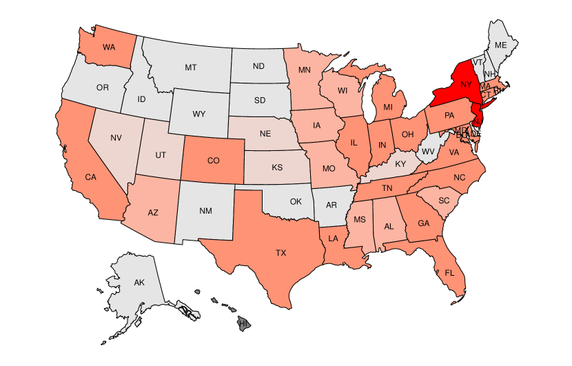
Figure 8. Clustering results based on the number of cumulative confirmed cases in 50 continental states in the US from 04/01/2020 to 05/15/2020.

For comparison, we also conduct an analogous analysis on a truncated study period from 04/01/2020 to 05/15/2020, around which business reopening starts over a large number of states. The clustering results are presented in Figure 8, and the cluster structure appears to be greatly different from that given in Figure 7. Essentially, the New York state and its neighbors are the epidemic centers for the period from 04/01/2020 to 05/15/2020, and the alterations in the cluster membership flag the significant impacts of reopening the business in accelerating the spread of the virus.

6. Forecasting

When forecasting the COVID-19 data using functional data approaches, we need to preserve the temporal dynamics among curves to maintain the forecasting ability, which leads us to the context of functional time series [FTS, 26].

6.1. Converting data into FTS

An FTS consists of a set of random functions collected over time. So far in the literature, there are two common formations of an FTS object. One treats an FTS as a segmentation of an almost continuous time record into natural consecutive intervals, such as days, months, or quarters. This is a conventional treatment for financial data [27]. The other treats it as a collection of curves over a time period, where the curves are not functions of time; see [12] for example. The major difference between these two formations is whether the continuum of each function is a time variable. In this section, we start with the number of nationwide cumulative confirmed cases of the COVID-19 in the US, where we define and convert the FTS using the first convention outlined above. Based on several reports on the COVID-19 pandemic [49, 76], the average incubation period of the coronavirus is about $7$ days, but the incubation period could last up to $14$ days for most of the cases. Therefore, we segment the number of cumulative confirmed cases into curves with time intervals of $14$ days. In line with the conventional treatment that segments a continuous curve into small intervals, we set the last value in one curve equal to the first value of the next.

Similar to the classical time series modeling, it is critical to appropriately handle the non-stationary data when modeling the FTS. To circumvent the issue of the non-stationarity in the COVID-19 data, we exploit the ideas from the literature dealing with FTS of share prices. In [18], the authors define the cumulative intraday returns (CIDR’s), and later in [30], a formal test that justifies the stationarity of CIDR’s curves has been developed. Here we convert the non-stationary cumulative confirmed case counts into stationary curves by calculating the daily growth rate in each curve:

$$r_{n,j}=100\times\bigl{[}\ln C_{n,j}-\ln C_{n,j-1}\bigr{]},$$ (7)

where $C_{n,j}$ denotes the number of confirmed cases on the $j$-th day of the $n$-th segment, for $j\in\{1,2,\ldots,14\}$, and $n\in\{1,2,\ldots,N\}$. Let $r_{n}{(t)}$ be the daily growth rates curve of the $n$-th segment, but values can only be observed at discrete time points $j$, such that $r_{n,j}=r_{n}{(t_{j})}$.

Under the functional data framework, we assume the neighboring grid points are highly correlated, and smoothing serves as a tool for regularization, such that we borrow information from the neighboring grid points [71]. When applying to the daily growth rate for the cumulative confirmed cases, we assume that the underlying continuous and smooth function $Y_{n}(t)$ is observed at discrete points with smoothing error $\epsilon_{n}(t_{j})$:

$$r_{n}(t_{j})=Y_{n}(t_{j})+\epsilon_{n}(t_{j});$$

see [31] for details on smoothing. After applying the test from [30], we find that the $p$-value is equal to $0.989$, suggesting the stationarity of the FTS with respect to the daily growth rates.

The rainbow plot proposed in [33] is effective in the visualization of the FTS. In a rainbow plot, functions that are ordered in time and colored with a spectrum of rainbow, such that functions from earlier times are colored in red, while the most recent ones are in violet. The rainbow plot captures the features of an FTS in two ways. Within each curve, the mode of variation reflects the pattern of the curve, and the ordering in color reveals the temporal dynamics over time.

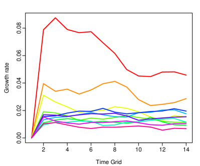
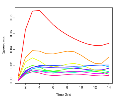
Figure 9. Functional time series for unsmoothed (left panel) and smoothed (right panel) growth rates of the cumulative confirmed cases of COVID-19 in the US.

Figure 9 presents the rainbow plot of both unsmoothed (left) and smoothed (right) growth rates of the cumulative confirmed cases of COVID-19 in the US from 04/04/2020 to 08/25/2020, leading to exactly $11$ functional curves. From Figure 9, we observe that all the curves share a similar temporal pattern, where the growth rate increases rapidly within the first four days, and then tapers off gradually. This coincides with a scientific finding that an infected person is most contagious early in the course of their illness [68]. Based on the color ordering in the rainbow plot, we see that the growth rate declines gradually from April to June, indicating the effectiveness of the practice of public health measures (including lock down policies implemented at the early stage of the outbreak), but it bounces back up again in July, flagging the effects of reopening.

In the rest of this section, we develop a forecasting scheme by considering a dynamic FPCA method that accounts for the temporal dynamics of the long-run covariance structure of the FTS. The forecasting is done through the dynamic FPCA scores. We use the root mean squared forecasting error and a nonparametric bootstrap approach to assess the accuracy of point and interval forecasts, respectively. We then apply the proposed scheme to forecast the number of confirmed cases in the US in the next $13$ days (the first day of the $14$-day prediction segment coincides with the last day of the study period).

6.2. Dynamic FPCA

The major critics of classical FPCA (c.f. Section 3.1) stem from its incapability of making forecasts as it only aims to reduce the dimension of data by maximizing the variances explained by eigenfunctions. The dynamic FPCA, however, manages to reduce dimension towards the directions mostly reflecting temporal dynamics [28]. To better accommodate the need of capturing the temporal dynamics among the FTS and making better forecast, we here adopt the dynamic FPCA method [28]. The primary difference between classical and dynamic FPCA is that in performing the eigenanalysis, we replace the variance-covariance function with the long-run covariance function.

For an FTS, the long-run covariance function, which is the functional analogue of the long-run covariance matrix in standard time series analysis, plays an important role in accommodating the temporal dependence among functions. We now give the definition of long-run covariance function. Let $\{Y_{i}(\tau),i\in\mathbb{Z}\}$ denote a sequence of stationary and ergodic functional time series, with $\tau$ being a bounded continuous variable. The long-run covariance function of $\{Y_{i}(\tau),i\in\mathbb{Z}\}$ is given by

$$\mathcal{C}(s,t):=\sum_{i=-\infty}^{\infty}\gamma_{i}(s,t),$$

where $\gamma_{i}(s,t)={\rm{\bf C}ov}(Y_{0}(s),Y_{i}(t))$. In practice, we need to estimate $\mathcal{C}(s,t)$ via a finite sample, i.e. $\{Y_{i}(\tau),i=1,2,\ldots,n\}$ for some integer $n<\infty$. We use the lag-window estimator proposed by [53] to estimate the long-run covariance function $\mathcal{C}(s,t)$:

$$\widehat{\mathcal{C}}(s,t):=\sum_{i=-\infty}^{\infty}\mathcal{K}\left(\frac{i}{h}\right)\widehat{\gamma}_{i}(s,t),$$ (8)

where $\mathcal{K}(i/h)$ is a kernel function assigning different weights to the auto-covariance functions with different lags, and the parameter $h$ is the bandwidth [3]. Typically, we assign more weights to the autocovariance functions of small lags and fewer to those of large lags. Here we use the “flat-top” type of kernels, as they provide smaller bias and faster rates of convergence [56]. For $k<1$, the flat-top kernel is given by

$$K\left(\frac{i}{h}\right)=\begin{cases}1,&\qquad 0\leq|i/h|<k;\\ \frac{|i/h|-1}{k-1},&\qquad k\leq|i/h|<1;\\ 0,&\qquad|i/h|\geq 1.\end{cases}$$

The selection of the bandwidth crucially affects the accuracy of estimation. Here we adopt an adaptive bandwidth selection procedure [61] to get an approximately optimal bandwidth for the subsequent estimation of the long-run covariance of FTS. The estimator $\widehat{\gamma}_{i}(s,t)$ is given by

$$\widehat{\gamma}_{i}(s,t)=\begin{cases}\frac{1}{n-i}\sum_{r=1}^{n-i}Y_{r}(s)Y_{r+i}(t),&\qquad i\geq 0;\\ \frac{1}{n-i}\sum_{r=1-i}^{n}Y_{r}(s)Y_{r+i}(t),&\qquad i<0.\end{cases}$$

The dynamic FPCA is done through the Karhunen-Loève expansion exactly the same as Equation (2), but the eigenvalues and eigenfunctions are estimated based on the eigenanalysis of $\widehat{\mathcal{C}}(s,t)$.

6.3. Forecasting based on scores

We use $m$ functional observations to get an $\ell$-step-ahead forecast by the method developed in [32]. Note that applying a univariate time series forecasting method to the score vector $\bm{\widehat{\xi}}^{(m)}_{k}=\{\widehat{\xi}_{1k},\widehat{\xi}_{2k}\ldots,\widehat{\xi}_{mk}\}$ gives the estimated $\widehat{\xi}_{m+\ell\,|\,m,k}$, then the estimate of the $\ell$-step-ahead forecast is given by

$$\widehat{Y}_{m+\ell\,|\,m}(t)=\widehat{\mu}(t)+\sum_{k=1}^{K}\widehat{\xi}_{m+\ell\,|\,m,k}\,\widehat{\phi}_{k}(t),$$

where $\widehat{\mu}(t)$ and $\{\widehat{\phi}_{k}(t),k=1,2,\ldots,K\}$ denote the estimated mean and FPCs, respectively.

For the application to the COVID-$19$ data, we forecast the daily number of the cumulative confirmed cases by the grid points on the forecasting curve. Without loss of generality, we consider the one-step-ahead forecast (i.e., $\ell=1$). Note that this procedure generates daily forecasts up to $13$ days, since by our assumption on the FTS conversion in Section 6.1, the first grid point on the curve is the same as that on the last day of the study period. By implementing the FTS converting procedures from 6.1, we obtain an FTS object consisting of $11$ functional curves. We create an expanding window analysis framework, and apply the proposed forecasting method to get multiple one-step-ahead forecasts on the growth rate curve. The details are deferred to Section 6.4.1.

6.4. Forecast accuracy evaluation

In this section, we introduce the methods that assess the prediction accuracy for point and interval forecasts. To make forecast for the number of confirmed cases in the US in the next $13$ days, we set $\ell=1$ throughout the section.

6.4.1. Point forecast

For a point forecast, We use the root mean square forecast error (RMSFE) to evaluate its accuracy:

$${\rm RMSFE}(j)=\sqrt{\frac{1}{N-n}\sum_{m=n}^{N-1}\left[C_{m+1}(j)-\widehat{C}_{m+1}(j)\right]^{2}},$$ (9)

where $N$ is the total number of segments in the FTS, $m$ is the number of curves used in forecasting, $C_{m+1}(j)$ is the number of confirmed cases at the ${j}$-th point on the ${(m+1)}$-th curve, and $\widehat{C}_{m+1}(j)$ is the corresponding forecast value. The RMSFE measures the discrepancy between the forecast and the actual value.

Given that there are $11$ functional curves in the study period, we start with the first $n=8$ curves to generate one-step-ahead point forecasts, and repeat this forecasting procedure by adding one curve at a time until the first $10$ curves are included, which gives us $(N-n=3)$ one-step-ahead forecasts in total. In other words, for each time point $j$, there are three forecast values. We choose $n=8$ as our starting point to ensure that an adequate number of curves are used for forecasting.

We adopt a standard forecasting approach through the autoregressive integrated moving average (ARIMA) model as a competing method. The forecasting results are presented in Figure 10, where the $y$-axis is the average of the RMSFE (scaled by $10$) of the three one-step-ahead point forecasts. We observe that the mean values of the RMSFE of FTS forecasts are consistently smaller than the counterparts of standard ARIMA, suggesting that the proposed FTS method is preferred.

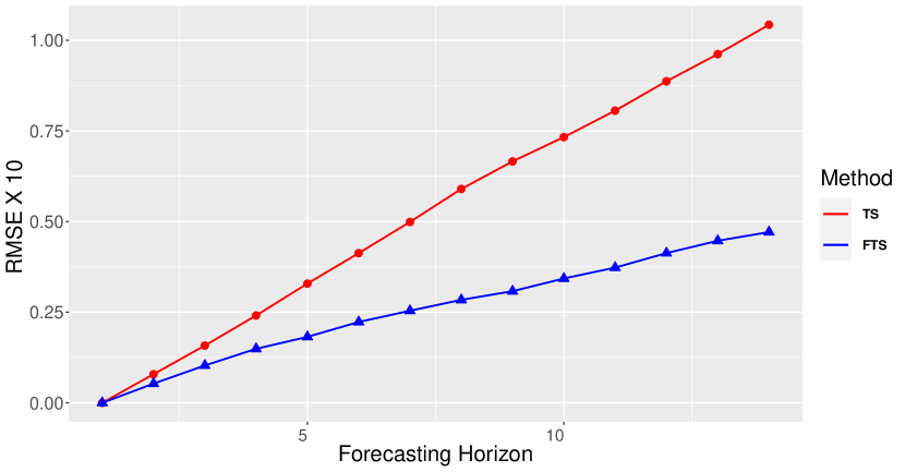
Figure 10. Average RMSFE values (scaled by $10$) for the FTS and the standard ARIMA method for the next $13$ days. The FTS method consistently outperforms the standard ARIMA. Note that the RMSFE curve starts from 0, corresponding to the assumption in Section 6.1 that the first day of the $14$-day prediction segment coincides with the last day of the study period.

6.4.2. Interval forecast

To better capture the uncertainty of point forecasts, we construct the associated prediction intervals in this section. In [4], uniform prediction intervals are generated using a parametric method, and later [66] suggests constructing pointwise prediction intervals via a nonparametric bootstrap method. The construction of the prediction intervals is based on in-sample-forecast errors, i.e., $\widehat{e}_{m+1\,|\,m}(j)=C_{m+1}(j)-\widehat{C}_{m+1}(j)$. Specifically, we generate a bootstrap sample (with replacement) of forecasting errors to obtain the upper and lower bounds, respectively denoted by $\eta^{\rm ub}(j)$ and $\eta^{\rm up}(j)$. Then we choose a tuning parameter, $\delta_{\alpha}$, such that

$${\rm\bf P}\left\{\delta_{\alpha}\times\eta^{\rm lb}(j)\leq\widehat{e}_{m+1\,|\,m}\leq\delta_{\alpha}\times\eta^{\rm ub}(j)\right\}=(1-\alpha)\times 100\%.$$

The one-step-ahead (pointwise) prediction interval is given by

$$\widehat{C}_{m+1}(j)+\delta_{\alpha}\times\eta^{\rm lb}(j)\leq C_{m+1}(j)\leq\widehat{C}_{m+1}(j)+\delta_{\alpha}\times\eta^{\rm ub}(j).$$ (10)

We use the interval scoring rules [19] to evaluate the accuracy of the pointwise interval forecasts. The interval score for the pointwise interval forecast (c.f. Equation (10)) at time point $j$ is given by

$$\begin{split}&S_{\alpha}\left[\widehat{C}_{m+1}^{\rm lb}(j),\widehat{C}_{m+1}^{\rm ub}(j);C_{m+1}(j)\right]\\ &=\left[\widehat{C}_{m+1}^{\rm ub}(j)-\widehat{C}_{m+1}^{\rm lb}(j)\right]+\frac{2}{\alpha}\left[\widehat{C}_{m+1}^{\rm lb}(j)-\widehat{C}_{m+1}(j)\right]\bm{1}\left\{\widehat{C}_{m+1}(j)<\widehat{C}_{m+1}^{\rm lb}(j)\right\}\\ &\quad{}+\frac{2}{\alpha}\left[\widehat{C}_{m+1}(j)-\widehat{C}_{m+1}^{\rm ub}(j)\right]\bm{1}\left\{\widehat{C}_{m+1}(j)>\widehat{C}_{m+1}^{\rm ub}(j)\right\},\end{split}$$

where $\bm{1}\left\{\cdot\right\}$ represents a standard indicator function, and the level of significance, $\alpha$, is conventionally set at $0.2$. A lower interval score suggests that the interval forecast is more accurate. The ideal scenario is that the actual values of $C_{m+1}(j)$ values lie between $\widehat{C}_{m+1}^{\rm lb}(j)$ and $\widehat{C}_{m+1}^{\rm ub}(j)$ for all $j$. The mean interval score over $(N-n)$ one-step-ahead forecasts becomes

$$\bar{S}_{\alpha}(j)=\frac{1}{N-n}\sum_{m=n}^{N-1}S_{\alpha}\Big{[}\widehat{C}_{m+1}^{\text{lb}}(j),\widehat{C}_{m+1}^{\text{ub}}(j);C_{m+1}(j)\Big{]}.$$

Figure 11 shows the mean interval scores (scaled by $10$) of the interval forecasts obtained from the FTS model versus the standard ARIMA model. The computation results reveal that the proposed FTS method outperforms the standard ARIMA.

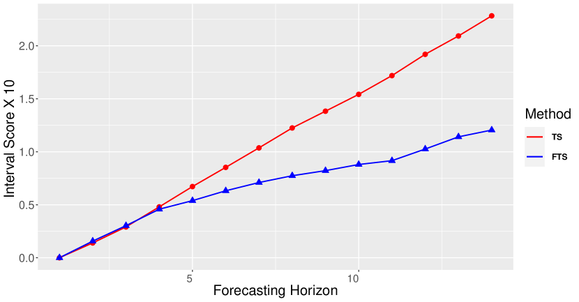
Figure 11. Average interval scores (scaled by $10$) for the FTS method and the standard ARIMA model for the next $13$ days. The FTS approach is preferred in that it produces smaller interval scores in most of the cases. Note that the RMSFE curve starts from 0, corresponding to the assumption in Section 6.1 that the first day of the $14$-day prediction segment coincides with the last day of the study period.

6.4.3. Future forecasts

We apply the proposed method to forecast the number of cumulative confirmed cases in the next $13$ days upon the last date of study period. Table 1 shows the predicted number and 80% confidence interval of nationwide cumulative confirmed cases (in thousands). In addition, the point forecasts and the associated 80% confidence bands for the cumulative confirmed cases in the US from 08/26/2020 to 09/07/2020 are depicted in Figure 12, where we also compare the prediction results with those generated from an ARIMA model.

From Table 1, we see that our FTS forecasts tends to slightly underestimate the total counts, but the actual count still falls within the prediction intervals. Such deviation may be due to the reopening of the schools starting from mid-August, leading to the surge in the cumulative confirmed cases nationwide. When comparing the FTS forecasting results with the ARIMA model in Figure 12, we see a narrower prediction interval for the FTS results, suggesting that it is preferred than the standard ARIMA model.

Table 1. Number of cumulative confirmed cases (in thousands) in the United States in the next 13 days (upon the last date of the study period).

Date	08/26	08/27	08/28	08/29	08/30	08/31	09/01
Actual	$5,839$	$5,884$	$5,931$	$5,975$	$6,009$	$6,045$	$6,089$
Forecasts	$5,815$	$5,840$	$5,863$	$5,884$	$5,907$	$5,935$	$5,970$
Lower Bound	$5,788$	$5,786$	$5,790$	$5,799$	$5,805$	$5,817$	$5,839$
Upper Bound	$5,843$	$5,902$	$5,948$	$5,981$	$6,010$	$6,049$	$6,090$
Date	09/02	09/03	09/04	09/05	09/06	09/07
Actual	$6,122$	$6,168$	$6,220$	$6,263$	$6,293$	$6,318$
Forecasts	$6,012$	$6,060$	$6,110$	$6,161$	$6,210$	$6,252$
Lower Bound	$5,865$	$5,885$	$5,913$	$5,946$	$5,976$	$6,006$
Upper Bound	$6,131$	$6,176$	$6,233$	$6,312$	$6,390$	$6,457$

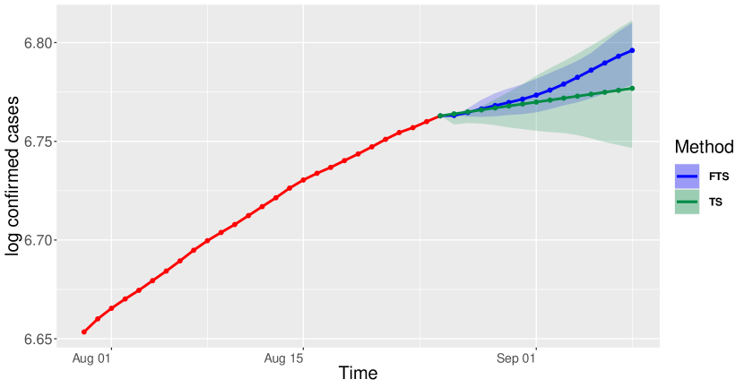
Figure 12. Point forecast and confidence bands for the number of total confirmed cases in the next 13 days (upon the last date of the study period)

7. Discussions

In this article, we conduct a functional data analysis of the time series data of COVID-19 in the US. Based on our results, it is evident that the practice of public health measures (e.g. “stay-at-home” order and mask wearing) helps reduce the growth rate of the epidemic outbreak over the nation. However, the implementation of the business reopening plans seems to have caused the rapid spread of the COVID-19 in some states, e.g. Texas and Florida.

We quantitatively assess the correlation between confirmed and death cases using the FCCA. Overall, we observe a high canonical correlation between confirmed and death cases, though the canonical variable scores vary from state to state. With the population size in each state carefully adjusted, we see that there is a substantial change in the cluster structure in the early and late times, and 05/15/2020 (the average date of business reopening across the states) appears to be a potential change point. Besides, states that are geographically close to the hot spots are likely to be clustered together, and population density (at state level) appears to be a critical factor affecting the cluster structure.

In addition, we also propose a forecasting scheme for the nationwide cumulative confirmed cases under the functional time series framework. Integrating information from the neighboring data point, the forecasting accuracy from the functional time series approach outperforms that from an ARIMA model. Forecasts are also made to the next $13$ days of the study period, and comparisons with the actual counts are provided. Although our method tends to produce smaller estimated counts for the next 13 days, the actual values still fall within the prediction intervals associated with our forecasts. It is also worthwhile noticing that such underestimation may indicate the effects of school reopening in accelerating the spread of the virus over the country.

References

- [1] Abdollahi, E., Champredon, D., Langley, J. M., Galvani, A. P. and Moghadas, S. M. (2020). Temporal estimates of case-fatality rate for COVID-19 outbreaks in Canada and the United States. Can. Med. Assoc. J. 192 E666–E670.
- [2] Abraham, C., Cornillon, P. A., Matzner-Løber, E. and Molinari, N. (2003). Unsupervised curve clustering using B-splines. Scand. J. Statist. 30 581–595. MR2002229
- [3] Andrews, D. (1991). Heteroskedasticity and autocorrelation consistent covariance matrix estimation. Econometrica 59 817–858.MR1106513
- [4] Aue, A., Norinho, D. D. and Hörmann, S. (2015). On the prediction of stationary functional time series. J. Amer. Statist. Assoc. 110 378–392. MR3338510
- [5] Biernacki, C., Celeux, G., and Govaert, G.. (2003). Choosing starting values for the EM algorithm for getting the highest likelihood in multivariate Gaussian mixture models. Comput. Statist. Data Anal. 41 561–575. MR1968069
- [6] Capra, W. B. and Müller, H.-G. (1991). An accelerated-time model for response curves. J. Amer. Statist. Assoc. 92 72–83. MR1436099
- [7] Carroll, C., Gajardo, A., Chen, Y. Dai, X., Fan, J. Hadjipantelis, P. Z., Han, K., Ji, H., Müeller, H.-G. and Wang, J.-L. (2020). fdapace: Functional Data Analysis and Empirical Dynamics. R package version 0.5.3, https://CRAN.R-project.org/package=fdapace.
- [8] Castro, P. E., Lawton, W. H. and Sylvestre, E. A. (1986). Principal modes of variation for processes with continuous sample curves. Technometrics 28 329–337.
- [9] Chen, W.-C. and Maitra, R. (2015). EMCluster: EM algorithm for model-based clustering of finite mixture Gaussian distribution. R Package, http://cran.r-project.org/package=EMCluster.
- [10] Chiou, J.-M. and Li, P.-L. (2007). Functional clustering and identifying substructures of longitudinal data. J. R. Stat. Soc. Ser. B Stat. Methodol. 69 679–699. MR2370075
- [11] Chiou, J.-M. and Li, P.-L. (2008). Correlation-based functional clustering via subspace projection. J. Amer. Statist. Assoc. 103 1684–1692. MR2724685
- [12] Chiou, J.-M. and Müller, H.-G. (2009). Modeling hazard rates as functional data for the analysis of cohort lifetables and mortality forecasting. J. Amer. Statist. Assoc. 104 572–585. MR2751439
- [13] Chung, F. R. K. (1997). Spectral Graph Theory. American Mathematical Society, Providence, RI. MR1421568
- [14] Dauxois, J., Pousse, A. and Romain, Y. (1982). Asymptotic theory for the principal component analysis of a vector random function: some applications to statistical inference. J. Multivariate Anal. 12 136–154. MR0650934
- [15] Dempster, A. P., Laird, N. M. and Rubin, D. B. (1977). Maximum likelihood from incomplete data via the EM algorithm. J. Roy. Statist. Soc. Ser. B 39 1–38. MR0501537
- [16] Fan, J. and Gijbels, I. (1996). Local Polynomial Modelling and its Application. Chapman & Hall, London, UK. MR1383587
- [17] Ferreira, L. and Hitchcock, D. B. (2009). A comparison of hierarchical methods for clustering functional data. Comm. Statist. Simulation Comput. 38 1925–1949. MR2751180
- [18] Gabrys, R., Horváth, L. and Kokoszka, P. (2010). Tests for error correlation in the functional linear model. J. Amer. Statist. Assoc. 105 1113–1125. MR2752607
- [19] Gneiting, T. and Raftery, A. E. (2007). Strictly proper scoring rules, prediction, and estimation. J. Amer. Statist. Assoc. 102 359–378. MR2345548
- [20] Grubaugh, N. D., Hanage, W. P. and Rasmussen, A. L. (2020). Making sense of mutation: What D614G means for the COVID-19 pandemic remains unclear. Cell https://doi.org/10.1016/j.cell.2020.06.040.
- [21] Hansen, L. P. (1982). Large sample properties of generalized method of moments estimators. Econometrica 50, 1029–1054. MR0666123
- [22] He, G., Müller, H.-G. and Wang, J.-L. (2003). Functional canonical analysis for square integrable stochastic processes. J. Multivariate Anal. 85 54–77. MR1978177
- [23] He, G., Müller, H.-G. and Wang, J.-L. (2004). Methods of canonical analysis for functional data. J. Statist. Plann. Inference 122, 141–159. MR2057919
- [24] He, W., Grace, Y. Y. and Zhu, Y. (2020). Estimation of the basic reproduction number, average incubation time, asymptomatic infection rate, and case fatality rate for COVID‐19: Meta‐analysis and sensitivity analysis. J. Med. Virol. https://doi.org/10.1002/jmv.26041.
- [25] He, X., Lau, E.H.Y., Wu, P. et al. (2020). Temporal dynamics in viral shedding and transmissibility of COVID-19. Nat. Med.. 26, 672–675.
- [26] Hörmann, S. and Kokoszka, P. (2010). Weakly dependent functional data. Ann. Statist. 38, 1845–1884. MR2662361
- [27] Hörmann, S. and Kokoszka, P. (2010). Functional time series, in T. S. Rao, S. S. Rao and C. Rao (Eds.) Handbook of Statistics 30 157–186, Elsevier, Amsterdam, North Holland.
- [28] Hörmann, S., Kidziński, Ł. and Hallin, M. (2015). Dynamic functional principal components. J. R. Stat. Soc. Ser. B. Stat. Methodol. 77, 319–348. MR3310529
- [29] Horváth, L., Kokoszka, P., and Reeder, R. (2012). Estimation of the mean of functional time series and a two-sample problem. J. R. Stat. Soc. Ser. B. Stat. Methodol. 75 103–122. MR3008273
- [30] Horváth, L., Kokoszka, P., and Rice, G (2014). Testing stationarity of functional time series. J. Econometrics 179 66–82. MR3153649
- [31] Hyndman, R. J., and Ullah, M. S. (2007). Robust forecasting of mortality and fertility rates: A functional data approach. Comput. Statist. Data Anal. 51 4942–4956. MR2364551
- [32] Hyndman, R. J., and Shang, H. L. (2009). Forecasting functional time series. J. Korean Statist. Soc. 38 219–221. MR2750317
- [33] Hyndman, R. J., and Shang, H. L. (2010). Rainbow plots, bagplots, and boxplots for functional data. J. Comput. Graph. Statist. 19 29–45. MR2752026
- [34] Hyndman, R.J., Booth, H., and Farah, Y. (2013). Coherent mortality forecasting: the product-ratio method with functional time series models. Demography 50 261–283.
- [35] Jacques, J. and Preda, C. (2013). Funclust: A curves clustering method using functional random variables density approximation. Neurocomputing 112 161–171.
- [36] Jacques, J. and Preda, C. (2014). Functional data clustering: a survey. Adv. Data Anal. Classif. 8 231–255. MR3253859
- [37] Jolliffe, I. T. (2002). Principal Component Analysis, 2nd ed. Springer-Verlag, New York, NY. MR2036084
- [38] Dong, E., Du, H., and Gardner, L. (2020). An interactive web-based dashboard to track COVID-19 in real time. The Lancet infectious diseases, 20(5), 533–534.
- [39] Jones, M. C. and Rice, J. A. (1992). Displaying the important features of large collections of similar curves. Amer. Statist. 46 140–145.
- [40] Karhunen, K.. (1946). Zur spektraltheorie stochastischer prozesse. Ann. Acad. Sci. Fennicae Ser. A. I. Math.-Phys. 34. MR0023012
- [41] Kaufman, L. and Rousseeuw, P. J. (1990). Finding Groups in Data: An Introduction to Cluster Analysis, 1st ed. Wiley-Interscience, Hoboken, NJ. MR2036084
- [42] Kosambi, D. D. (1943). Statistics in function space. J. Indian Math. Soc. 7 76–88. MR0009816
- [43] Lee, G. and Scott, C. (2012). EM algorithms for multivariate Gaussian mixture models with truncated and censored data. Comput. Statist. Data Anal. 56 2816–2829. MR2915165
- [44] Leurgans, S. E., Moyeed, R. A. and Silverman, B. W. (1993). Canonical correlation analysis when the data are curves. J. Roy. Statist. Soc. Ser. B 55 725–740. MR1223939
- [45] Li, Y. and Hsing, T. (2010). Uniform convergence rates for nonparametric regression and principal component analysis in functional/longitudinal data. Ann. Statist. 38 3321–3351. MR2541589
- [46] Li, Y., Wang, N., and Carroll, R. J.. (2013). Selecting the number of principal components in functional data. J. Amer. Statist. Assoc. 108 1284–1294. MR3174708
- [47] Liu, B. and Müller, H.-G. (2009). Estimating derivatives for samples of sparsely observed functions, with application to online auction dynamics. J. Amer. Statist. Assoc. 104 704–717. MR2541589
- [48] Loève, M.. (1955). Probability Theory: Foundations, Random Sequences. D. Van Nostrand, Company, Inc., Princeton, NJ.
- [49] McAloon, C., Collins, Á, Hunt, K. et al. (2020). Incubation period of COVID-19: A rapid systematic review and meta-analysis of observational research. BMJ Open, 10 e039652.
- [50] McLachlan, G. and Peel, D. (2000). Finite Mixture Models. Wiley-Interscience, New York. MR1789474
- [51] Newey, W. K. and West, K. D. (1987). A simple, positive semi-definite, heteroskedasticity and autocorrelation consistent covariance matrix. Econometrica 55 703–708. MR0890864
- [52] Ommer, S. B., Malani, P. and del Rio, C. (2020). The COVID-19 andemic in the US: A clinical update. JAMA 323 1767–1768.
- [53] Panaretos, V. M. and Tavakoli, S. (2013). Fourier analysis of stationary time series in function space. Ann. Statist. 41 568–603. MR3099114
- [54] Peirlinck, M., Linka, K., Costabal, F. S. and Kuhl, E. (2020). Outbreak dynamics of COVID-19 in China and the United States. Biomech. Model. Mechanobiol. https://doi.org/10.1007/s10237-020-01332-5.
- [55] Peng, J. and Müller, H.-G. (2008). Distance-based clustering of sparsely observed stochastic processes with applications to online auctions. Ann. Appl. Stat. 2 1056–1077. MR2516804
- [56] Politis, D. N. and Romano, J. P. (1996). On flat-top kernel spectral density estimators for homogeneous random fields. J. Statist. Plann. Inference 51 41–53.
- [57] Ramsay, J. O. (1982). When the data are functions. Psychometrika 47 379–396. MR0691828
- [58] Ramsay, J. O. and Dalzell, C. J. (1991). Some tools for functional data analysis. J. Roy. Statist. Soc. Ser. B 53 539–572. MR1125714
- [59] Ramsay, J. O. and Silverman, B. W. (2002). Applied Functional Data Analysis: Methods and Case Studies. Springer-Verlag, New York, NY. MR1910407
- [60] Ramsay, J. O., Graves, S. and Hooker, G. (2020). fda: Functional Data Analysis. R package version 5.1.4, https://CRAN.R-project.org/package=fda.
- [61] Rice, G. and Shang, H. L. (2017). A plug-in bandwidth selection procedure for long-run covariance estimation with stationary functional time series. J. Time Series Anal. 38 591–609. MR3664648
- [62] Shibata, R. (1981) An optimal selection of regression variables. Biometrika 68 45–54. MR0614940
- [63] Scotto, M. G., Wei, C. H. and Gouveia, S. (2015). Thinning-based models in the analysis of integer-valued time series: a review. Stat. Model. 15 590–618. MR3441230
- [64] Shang, H. L. (2014). A survey of functional principal component analysis. AStA Adv. Stat. Anal. 98 121–142. MR3254025
- [65] Shang, H. L.(2017). Forecasting intraday S&P 500 index returns: A functional time series approach, Journal of forecasting 36 741–755.
- [66] Shang, H. L. (2018). Bootstrap methods for stationary functional time series. Stat. Comput. 28 1–10. MR3741633
- [67] Shang, H. L., Yang, Y. and Kearney, F. (2019).Intraday forecasts of a volatility index: functional time series methods with dynamic updating. Ann. Oper. Res. 282 331–354. MR4019243
- [68] Siordia, J. A. Jr. (2020). Epidemiology and clinical features of COVID-19: A review of current literature. J. Clin. Virol., 127 104357.
- [69] Thorndike, R. L. (1953). Who belongs in the family? Psychometrika 18 267–276.
- [70] Ullah, S. and Finch, C. F. (2013). Applications of functional data analysis: a systematic review. BMC Med. Res. Methodol. 13 43.
- [71] Wang, J.-L., Chiou, J.-M. and Müller, H.-G. (2016). Functional data analysis. Ann. Rev. Stat. Appl. 3 257–295.
- [72] Yang, W., Müller, H.-G. and Stadtmüller, U. (2011). Functional singular component analysis. J. R. Stat. Soc. Ser. B Stat. Methodol. 73 303–324. MR2815778
- [73] Yao, F., Müller, H.-G. and Wang, J.-L. (2005). Functional data analysis for sparse longitudinal data. J. Amer. Statist. Assoc. 100 577–590. MR2160561
- [74] Yao, F. and Müller, H.-G. (2005). Functional quadratic regression. Biometrika 97 49–64. MR2594416
- [75] Zhang, X. and Wang, J.-L. (2016). From sparse to dense functional data and beyond. Ann. Statist. 44 2281–2321. MR3546451
- [76] Zhang, P., Wang, T. and Xie, S. X. (2020). Meta-analysis of several epidemic characteristics of COVID-19. J. Data Sci. 18 536–549.