Dynamics of delayed neural field models in two-dimensional spatial domains
Abstract
Delayed neural field models can be viewed as a dynamical system in an appropriate functional analytic setting. On two dimensional rectangular space domains, and for a special class of connectivity and delay functions, we describe the spectral properties of the linearized equation. We transform the characteristic integral equation for the delay differential equation (DDE) into a linear partial differential equation (PDE) with boundary conditions. We demonstrate that finding eigenvalues and eigenvectors of the DDE is equivalent with obtaining nontrivial solutions of this boundary value problem (BVP). When the connectivity kernel consists of a single exponential, we construct a basis of the solutions of this BVP that forms a complete set in . This gives a complete characterization of the spectrum and is used to construct a solution to the resolvent problem. As an application we give an example of a Hopf bifurcation and compute the first Lyapunov coefficient.
Key words. Neural Field Equations, Delay Differential Equations, Sturm-Liouville Problems, Completeness of Set of Exponential Functions, Completeness of Eigenfunctions, Hopf bifurcation
AMS subject classifications. 34K06, 34K08, 92C20, 34B24, 42C15, 42C30, 46A35, 46B15
1 Introduction
Neural field models are based on the seminal work of Wilson and Cowan [21, 22] on the dynamical properties of two populations of excitatory and inhibitory neurons. Instead of taking individual spiking neurons, a neural field model is obtained by spatial and temporal averaging of the membrane potential across a population of neurons over a time interval. The interactions between neurons across synapses are modelled as a convolution over a so-called connectivity kernel and with a nonlinear activation function. In the work of Amari [1], this model is consolidated into a single integro-differential equation. Later Nunez [11] expanded this work by including the transmission delays of the signals between neurons. These neural fields prove to be useful to understand various neural activity in the cortex and other parts of the brain [4, 2, 3, 18].
Delayed neural field models take the form of an integro-differential equation with space dependent delays. By choosing the proper state space, they can be reformulated as an abstract delay differential equation [16, 15], where many available functional analytic tools can be applied. When the neuronal populations are distributed over a one-dimensional domain and a special class of connectivity functions is considered, a quite complete description of the spectrum and resolvent problem of the linearized equation is known [5, 16]. Recently, this model has been extended by including a diffusion term into the neural field, which models direct, electrical connections, [15]. We analyze the evolution of a delayed neural field equation corresponding to a single population of neurons on a two-dimensional spatial domain. For a summary of some extensions of neuronal activity models from one to two dimensions cf. [3] and references therein. Numerical methods developed for the efficient and accurate time simulation of neural fields on higher dimensional domains can be found in [7, 9, 12]. Moreover, numerical studies of the non-essential spectrum of abstract delay differential equations are also available, [19]. Analytic results in this framework, to the best of our knowledge, cannot be found in the literature. In [20], Visser et al. have characterized the spectrum for a neural field with transmission delays on a spherical domain and computed normal form coefficients of Hopf and double Hopf bifurcations. In this paper we give an analytic description of the spectrum of the linearized problem on a rectangle. Due to our choice of the connectivity kernel and the transmission delays, it is possible to transform the characteristic equation of the DDE into a linear PDE.
The first step towards finding a solution is to determine the characteristic polynomial for the PDE. We define an equivalence class on the complex plane characterized by the roots of this polynomial. It is then possible to give a partition of the exponential solutions of the PDE corresponding to these equivalence classes. Moreover, when we consider finite linear combinations of exponential solutions of the PDE, we can derive further conditions, identified as boundary conditions. When the connectivity kernel consists of a single exponential, modeling a population with inhibitory neurons, we give a complete characterization of the solution of this boundary value problem (BVP), hence obtain the eigenfunctions corresponding to the eigenvalues of the DDE. In this special connectivity case, the solution of the BVP can be given using the separation of variables, which leads to two Sturm-Liouville problems on one dimensional domains. The vector space of separable solutions form a complete basis in the space of square integrable functions on the rectangle. Using this unique basis expansion, we give a complete characterization of the spectrum and resolvent and this is one of the main results of this paper.
The paper is organized as follows. In Section 2, we summarize the functional analytic setting from [16, 15] that casts the integro-differential equation into an abstract DDE. It is shown in Section 3 how to obtain an explicit representation of some eigenvectors of the linearized problem for a particular choice of connectivity function, expressed as a finite linear combination of exponential functions. This type of connectivity models a mixed population of interacting excitatory and inhibitory neurons. In Section 4 we give a complete description of the spectrum and resolvent problem when the connectivity is a single exponential. Finally, we show an example of a Hopf bifurcation in Section 5.
The mathematical model for neural fields with space-dependent delays is as follows. Consider populations consisting of neurons distributed over a bounded, connected domain For each the variable denotes the membrane potential at time averaged over those neurons in the th population positioned at These potentials are assumed to evolve according to the following system of integro-differential equations
| (1) |
for The intrinsic dynamics exhibits exponential decay to the baseline level as The propagation delays measure the time it takes for a signal sent by a type- neuron located at position to reach a type- neuron located at position The function represents the connection strength between population at location and population at location at time The firing rate functions are For the definition and interpretation of these functions we refer to [17].
2 Functional analytic setting
In this paper we analyze the evolution of a single population of neurons, in a bounded two-dimensional domain
| (2) |
Note that we will only deal with autonomous systems, hence, the connectivity does not depend on time. We assume that the following hypotheses are satisfied for the functions involved in the system, (as in [16]): the connectivity kernel the firing rate function and its th Fréchet derivative is bounded for every and the delay function is non-negative.
From the assumption on the delay function we may set
We define the Banach spaces and For and for we write and its norm is given by
where From the assumption on the connectivity kernel, it follows that it is bounded in the following norm
We use the traditional notation for the state of the system at time
Define the nonlinear operator by
| (3) |
Then the neural field equation (2) can be written as a DDE as
| (4) |
where the solution is an element of Similarly, we have the state of the solution at time defined as It was shown in [16] that under the above assumptions on the connectivity, the firing rate function and delay, the operator is well-defined and it satisfies a global Lipschitz condition.
Let be the Fréchet derivative of at the steady state , given as
We assume that such that (2) admits the trivial equilibrium. Then the linearized problem around the equilibrium is
| (5) |
The solution of the linear problem defines a strongly continuous semigroup on generated by , where
We denote by and the resolvent set, the spectrum and the point spectrum of respectively.
3 Spectral properties of the linearized equation
In this section, we study the spectral properties of the linearized equation (5) when the space domain is the rectangle and the connectivity kernel is a finite linear combination of exponentials of the form
| (6) |
where , such that is real-valued. Moreover, the delay function is
| (7) |
First we deal with the essential spectrum, , the part of the spectrum which is invariant under compact perturbations. We can leverage the fact that is compact with Theorem 27 of [15] to find .
The remaining point spectrum consists of eigenvalues with a finite-dimensional eigenspace. Due to Proposition VI.6.7 of [6], eigenvectors for delay equations have the form
| (8) |
with the eigenvalue and a non-trivial solution of the characteristic equation
| (9) |
with the linear operators given by
| (10) |
with and . The integral equation is a Fredholm integral equation of the second type acting on multivariate functions.
3.1 From an integral equation to a partial differential equation
The main idea to solving is to transform the integral equation to a PDE. Some exponential solutions of the PDE, with some conditions on the boundary, are then again solutions of the characteristic equation (9).
First we establish that the eigenvectors are smooth.
Proposition 3.1.
For any the solution of is
Proof.
The range of is contained in for all and all . Hence, any solution of is in . The result follows by induction. ∎
For the remaining part of this section we assume that , so all differential operators applied to are well-defined.
Differentiating the kernel functions in the integral equation (9) in the distributional sense w.r.t. one of the spatial variables yields
| (11) |
with . This motivates the introduction of the differential operators
| (12) |
When applying to the integral operator defined in (10), we obtain
| (13) |
So acts like a left-inverse of . Using this key property, we find that applying the operator to the characteristic equation (9), leads a the linear constant coefficient PDE
| (14) |
We can only generically expect to find solutions of this PDE which are exponential functions or linear combinations of exponential solutions. So we first look for a solution of this PDE in the form
| (15) |
This leads to the characteristic polynomial equation , with given by
| (16) |
The characteristic polynomial is symmetric under interchanging and negating and , i.e., .
The next proposition shows that there are only a few such that has a nontrivial solution when or . We exclude these as they cause difficulties in later theorems.
Proposition 3.2.
Define the set by
Then and for all and if and only if .
Proof.
For and we have that
Clearly these are nonzero if and only if . ∎
Consequently, for we have that is equivalent to
| (17) |
We now want to use solutions of the PDE (14) to construct an eigenvector which solves (9). Unfortunately the set of the roots of the polynomial is uncountable. So we restrict ourselves to finite linear combinations of exponential solutions. For these finite linear combinations we can construct an explicit condition for solving (9) that only uses values of at the boundary of . In the next theorem we drop the -dependence of the operators for clarity.
Theorem 3.3.
Let such that . Let be a finite linear combination of exponential solutions of the PDE (14), i.e. , with a finite subset of and , where are some constants in .
Then if and only if
| (18) |
Proof.
We can further evaluate the condition in (18) using integration by parts. The operator on the left hand side of (19) is a operator that acts on and its normal derivatives at the boundary of . Hence, we will refer to (18) as the boundary condition from this point forward.
For a general the following holds for
| (19) |
where
| (20) |
and
| (21) |
Finding eigenvectors with an arbitrary number of exponentials is still hard. However, we can show that if we have such an eigenvector, then a subset of at most exponentials form also an eigenvector. To prove this, we first need the following equivalence relation.
Definition 3.4.
For every define the relation on as follows: For
| (22) |
Proposition 3.5.
Let , then the relation defines an equivalence relation on
Proof.
By definition is reflexive and by the symmetry of , is also symmetric.
For every , we can construct an equivalence class . Using this equivalence relation we can partition the null-space of into the following sets.
Definition 3.6.
For every , define the set as
| (24) |
Proposition 3.7 (Partition principle).
Let and . For all and , and .
Proof.
Let and . Suppose , then and hence by Proposition 3.5, . A similar reasoning holds when , so we have proven this statement by contradiction. ∎
This property makes us able to split the boundary condition (18) into multiple independent conditions corresponding to a single set . Note that the above property does not hold for any non-empty, proper subset of .
Proposition 3.8.
Suppose and that is a finite linear combination of exponential solutions as in Theorem 3.3, which solves . Then for all for which there exists a such that , with a finite subset of ,
| (25) |
Proof.
Let and as in Theorem 3.3. Using (19)-(3.1) we find that for all and
with
| (26) |
We note that is a linear combination of exponentials and and that of .
As , we get by Proposition 3.2 that for all , for . Furthermore, as , by Proposition 3.7, for all , and . Hence the elements of the set
are linearly independent.
We conclude that the terms
are linearly independent. As satisfies the boundary conditions (18), these should vanish. ∎
Generically, a polynomial of degree has distinct roots. As we show in the proposition below, this implies a generic representation of .
Proposition 3.9.
Let and suppose that the equivalence class has distinct elements . Then and for .
Proof.
For given , is a polynomial of order in . So if has distinct elements, then must have distinct solutions , which are not equal to , so we can define . Furthermore as must be distinct from , this implies that for . ∎
The sum of exponentials corresponding to can equivalently be expressed as
| (27) |
where we require that for . The coefficients form the matrices with a zero diagonal. The superscripts refer to coefficients of even and odd functions of and , respectively.
We define the matrices with elements
| (28) |
for . The superscripts refer to even and odd functions in , respectively.
Proposition 3.10.
Let and suppose that the equivalence class has distinct elements. Then
| (29) |
implies that
| (30) |
Proof.
For this proof we drop the dependency on and . We do some calculations beforehand using (3.1) and (3.1):
hold for . Now we expand (29) and (30) as
and
Since , we have by Proposition 3.2 that and for and , where . Since has elements we have by Proposition 3.9 that for , where . Hence all the terms above of cosine hyperbolic and sine hyperbolic in and are linearly independent and hence all the sums on the right have to be zero to satisfy the conditions.
Corollary 3.11.
Let and suppose that the equivalence class has distinct elements. Then if and only if
| (33) |
We can conclude that finding eigenvectors comes down to finding non-trivial solutions to the matrix equations (31). The problem is that for to be non-zero, there are equations and unknowns in and and , in total unknowns. When then the number of equations and unknowns are the same. This special case will be treated separately in the next section. When then the number of conditions is larger than the number of unknowns. However, we can reduce the amount of equations to some extent. To illustrate this, we consider and distinguish two cases: and .
When , it means that we can write , where are non-trivial solutions of . To satisfy the condition that has a zero diagonal, one of or has to have two zero elements. Without loss of generality, suppose that . Then implies that and , or equivalently,
| (34) |
Subtracting these equations and using that , we get that . Substituting this back into (34) implies that , which is not possible simultaneously with . Hence must be at least 2.
Due to the Sylvester’s rank inequality, and . Hence implies that . In this case it is then possible to construct an explicit solution for , so the condition , is also sufficient.
Requiring that , i.e., the two rows of are linearly dependent, gives the following conditions
Under the same assumption on , for each of the matrices there are 4 conditions and we have in total 6 unknowns, and the constants for each matrix. Hence this system is overdetermined and therefore has no generic solution.
However, when the matrices and are the same and this means 4 conditions and 4 unknowns. Therefore, with a Newton method we can find such that and from that we can explicitly find a non-trivial solution of the form
This works similarly for and . Obtaining however a non-trivial or still requires 8 conditions to be satisfied and it is thus non-generic.
In conclusion, there are only generic eigenvectors which are a (finite) sum of exponentials if . Otherwise, generic eigenvectors for (and maybe also some for ) are solutions to (9) which are not a sum of exponentials. In general, there is no guarantee that solutions of these integral equations can be expressed analytically.
4 Single exponential connectivity
In this section, we consider the case when the connectivity kernel in (6) is a single exponential, i.e., . In contrast to , in this case we can find a complete characterisation of the spectrum. Using the results of Section 3, we formulate the boundary value problem and give an analytic representation of the solution. After having described the spectrum of the linearized neural field equation, we solve the resolvent problem for this special case and using these results, we give an example of a Hopf bifurcation in the next section. For notational simplicity, we drop the subscripts of the operators.
As shown in Section 3, we can transform the integral equation (9) into a PDE using the fact that . In the next theorem we state that, for the characteristic integral equation of the DDE is equivalent to a PDE with an additional (boundary) condition.
Theorem 4.1.
Let such that and let such that and . Then we have the following equivalence
| (35) |
Moreover, for any we get that
| (36) |
Proof.
Let such that and let , such that . The smoothness condition on implies that
| (37) |
is well defined. Using in (36) gives (35), so we only prove (36). For the remaining part of this proof we will drop the dependency on for clarity.
First we apply the operator and to
Suppose that . Then from the equations above we get that
and that .
Conversely, suppose that and that . Then
and hence as . ∎
Note that, for the set of where holds, has a two-sided inverse . Using (19), we can write in terms of derivatives of at the boundary of . In the next lemma we can see that, under some conditions, we can interpret the right-hand side of (35) as a boundary value problem with a Robin-type boundary condition.
Lemma 4.2.
Let such that . Then
| (38) |
implies that , where is the outward normal derivative to the boundary of .
If and , where , and , for all , then also implies (38).
Proof.
From (19),we can write in terms of the operators and as
| (39) |
The first statement then immediately follows from the definition of and in (3.1) and (3.1), respectively.
Conversely, assume that , with and as in the second statement of the lemma. Then we can write and as
and
Using the fact that and for all , we can reason by linear independence that each term of should vanish and hence (38) holds. ∎
We can rewrite the PDE as
| (40) |
So is an eigenvalue of the original DDE, when is an eigenvalue of with a domain of functions which satisfy the boundary condition .
4.1 Eigenvalues and eigenvectors
We can use Corollary 3.11 and the matrix equations of (31) to find some eigenvalues with eigenvectors which are a sum of exponentials. But first we take a look at the set of resonances .
From the definition of in Proposition 3.2 we see that reduces to for . When , i.e. , any solution to is constant, as
Hence is an eigenvalue if and only if
We can now characterize the eigenvalues , i.e., those values for which has a non-trivial solution.
Theorem 4.3.
Let such that and let such that with , where
| (41) |
If , then is an eigenvalue with the eigenvector .
If , then is an eigenvalue with the eigenvector .
If , then is an eigenvalue with the eigenvector .
If , then is an eigenvalue with the eigenvector .
Proof.
We can directly apply Corollary 3.11. More specifically the matrix equations (31) hold. Without loss of generality, we set , leaving only as a variable satisfying . For , has the following structure
Hence the equations in decouple, so we can solve for and independently. Without loss of generality we can set , which gives the following set of equations
Set to an arbitrary non-zero complex value, leaving the remaining conditions in the theorem. From (27), we get that the eigenvector in this case has the form .
Choosing a different matrix from to be nonzero, gives the remaining conditions in the theorem. ∎
The two equations in the theorem above, together with the condition form a set of three equations with three unknowns , which can be solved generically. So for , we can indeed find generic eigenvectors which are exponentials.
Also note that inserting into the right-hand side of (35) gives exactly for the PDE and for the boundary condition.
We claim that with this theorem we have characterized all the eigenvalues. We will prove this by showing that we can construct a resolvent for all other values . We do this by first constructing a basis of the eigenfunctions of the operator that satisfy the boundary conditions.
4.2 Sturm-Liouville problems arising from neural field equations
Solving the characteristic equation is equivalent to finding the solution of the boundary value problem (40) and (38). Throughout this section we omit the -dependence of and for clarity. We seek solutions of the PDE (40) in the separated variable form
| (42) |
Inserting this form into (40), we obtain
Dividing by and denoting and ,
or equivalently,
Letting be the common constant value, we obtain two Sturm-Liouville problems (SLP) with Robin type boundary conditions
| (43) |
and
| (44) |
where . Note that the boundary conditions follow from Lemma 4.2.
Let us introduce the coordinate transformation into the SLP (43) and obtain
| (45) |
Equivalently, the SLP is
| (46) |
First, we check separately the case when is an eigenvalue. Here there are two cases, either , then the problem reduces to the homogeneous Neumann boundary conditions and the eigenfunction corresponding to the zero eigenvalue is , or , then is a solution.
We study the SLP (46) by first rewriting it to a first order system as
with
The boundary conditions can be reformulated as
| (47) |
Let be the matrix solution of the initial value problem
with the identity matrix, and define the following transcendental function, also called characteristic function for the SLP
| (48) |
Let us recall the following lemma that shows that the zeroes of are precisely the eigenvalues of the SLP.
Lemma 4.4 (Lemma 3.2.2, [24]).
A complex number is an eigenvalue of the BVP (46) if and only if . Furthermore, the geometric multiplicity of the eigenvalue is equal to the number of linearly independent vector solutions of the linear algebra system
To compute choose the branch , and obtain
| (49) |
Hence the characteristic function is
| (50) |
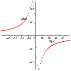
Since , if is a root of the entire function , then so is . According to Lemma 4.4, the eigenvalues of the SLP (46) are exactly the roots of the equation (50). Note that this equation has infinite but countable number of roots, these are all simple and have no finite accumulation point in . A few roots of the SLP (43) are plotted in Figure 1 for and .
4.2.1 Eigenvalues and completeness of exponentials
In this section we describe the location of the eigenvalues of the SLP in the complex plane and an interesting consequence which results from this distribution of the eigenvalues, i.e., the sets of exponential functions and used to construct the solutions of the corresponding Sturm-Liouville problems (43) and (44) are complete in and , respectively. There is an extensive literature on the completeness of sets of complex exponential functions over finite intervals, see e.g., [13, 14, 23] and the references therein. In Section 4.2.2, we will construct the eigenfunctions corresponding to the eigenvalues of the SLP using these exponentials. Note here that although we were not successful in proving the completeness of the eigenfunctions in the corresponding Banach space of continuous functions, but only in the larger space of square integrable functions, we were able to overcome this in Section 4.3 and give a complete characterization of the spectrum of the DDE.
Let us introduce some notations. The set of zeroes of a function is denoted by
| (51) |
and the number of zeroes of by . In general, the cardinality of a set will be denoted by .
Using the coordinate transformation introduced in (45), we will show that the set of complex exponentials is complete in , where is the characteristic function (50). Since , if we denote the roots of for which by , then are also roots of . This sequence is called symmetric and we can denote it by .
In the following theorem, we summarize two important results from [23] that we will use to prove the completeness of sets of exponentials.
Theorem 4.5.
Let be a sequence of complex numbers.
-
(1)
If
(52) then the system is complete in , for each closed subinterval of .
-
(2)
The completeness of the system in is unaffected if some is replaced by an other (different from all) number ([23], Theorem 7, Chapter 3).
The conditions in (52) show that all lie ”near” the real axis. Our next two lemmas show that almost all roots of satisfy these conditions.
Lemma 4.6.
Consider the characteristic equation in (50). For every there exists and such that the followings hold
-
(a)
for all there is a unique , such that .
-
(b)
Proof.
We prove part (a) first. Let us rewrite in (50) as
| (53) |
Note that if then . Since has zeroes at and poles at , where , consider the following stripe in the complex plane
Let be a closed simple curve around , with interior , that is contained entirely in and avoids . The complement domain of in is denoted by . Use the following two observations. First,
| (54) |
and second, that
| (55) |
The limit (55) yields that there exists an , such that
Let be the shift of by , where and . Since
| (56) |
we can apply Rouché’s theorem to conclude that the number of zeros of in the interior of equals the number of zeros of . Due to the choice of , we obtained that has exactly one zero inside , which completes the proof of part (a) of the lemma.
To prove part (b), we study the zeroes of , or equivalently, the solutions of
| (57) |
When , the roots are , where . Note that in this case the SLP reduces to the Neumann problem and we know that the system is complete in .
Let us fix and let . Using the trigonometric relation
we have that, for ,
| (58) |
Moreover, if , then for all . The limit
suggests to take for given a closed curve around the origin, such that is small on this curve and it is far from the poles of . Hence, define a square around the origin as
Then
| (59) |
Therefore, there exists such that the poles of , that is , are contained in the interior of and for all , and is large enough such that
| (60) |
Then we can apply Rouché’s theorem, which says that in the interior of
where counts the number of poles of the corresponding functions. The left hand side equals 1 and on the right hand side
| (61) |
since are in the interior of . Hence, . Since has the same zeroes as , except , we can conclude that in the interior of , which completes part (b) of the lemma.
Therefore, letting is then suitable for both parts of the lemma. ∎
Corollary 4.7.
An immediate consequence of Lemma 4.6 is that
Lemma 4.8.
Consider the set , with given in (50). Then
| (62) |
Proof.
First, note that the set cannot have finite accumulation points. If all eigenvalues , are real, then (62) holds.
If the assertion is not true, then there exists a subsequence , such that , where . If we insert this into (53), we obtain
Taking the limit , we obtain that the left hand side converges to and the right hand side to , which leads to a contradiction. ∎
The main result of this section is the following theorem.
Theorem 4.9 (Completeness theorem).
Let , where is the characteristic function in (50). Then the set is complete in .
Proof.
From Lemma 4.6 it follows that there exists an such that
| (63) |
Moreover, since , let us replace of these roots by in the exponentials, that is by . The new set of exponentials will now satisfy the condition on the real part of the eigenvalues in (52). This, in combination with (62), implies that this set is complete in each closed subinterval of . According to part (2) of Theorem 4.5, if we replace the set by the corresponding finite set , then the completeness will be unaffected. ∎
This way we have shown that the set is complete in and analogously, we can show that the set is complete in . Then forms a complete set in .
4.2.2 Completeness of the eigenfunctions
In [10], the solution of SLP problems are discussed in a more general framework. Based on these results, we construct the eigenfunctions corresponding to the eigenvalues of the SLP and state their completeness in the space of square integrable functions. As a consequence, the eigenfunctions of the the operator , which are the separable solutions of the BVP (35), form a complete basis in . In Section 4.3 we show that this is sufficient to give a complete characterization of the spectrum of the DDE and to solve the resolvent problem in Section 4.3.
Using the results of the previous section, we can conclude that the eigenvalues of the SLP (46) with large absolute value are of the form
| (64) |
Note that this was also shown in [10]. Following the ideas and results in [10], we can construct the following solutions of the differential equation in (46)
| (65) | ||||
| (66) |
Moreover, since
if is a root of the characteristic function (50), then and solve the SLP (46) and they are called eigenfunctions corresponding to the eigenvalue , with .
Theorem 4.10 (Theorem 1.3.2., [10]).
The system of eigenfunctions and generalized eigenfunctions of the BVP (46) is complete in the space and constitutes there a Riesz basis.
Since all roots of the characteristic function are simple, we do not have generalized eigenfunctions for this problem. The linear span of the eigenfunctions constructed from the solutions and coincide. It is therefore sufficient to consider the eigenfunctions derived from hence, we will omit the subscript.
If , with , then the corresponding eigenfunctions will be denoted as
| (67) |
where
and the following identity holds
From here, it follows that if is a root of the characteristic function, then either or . From (64) it follows that the roots of are those roots of that have the form and the corresponding eigenfunctions we call odd eigenfunctions and they have the form
| (68) |
Similarly, the roots of have the form and the corresponding eigenfunctions are called even eigenfunctions
| (69) |
Summarizing, Theorem 4.10 implies that the set of even and odd eigenfunctions is complete in .
In the original coordinate system the eigenfunctions are
| (70) |
where
and the following holds
Using the same argument as before, if is a root of , then either or vanish there. Note that, these are precisely the conditions we obtained earlier in Theorem 4.3. We can conclude that the system is complete in , with
| (71) |
Note that the following relations hold
Analogous result holds for the eigenvalues and corresponding eigenfunctions of the SLP (44). Returning to the original problem of solving the BVP (40) and (38) by separating the variables, we can summarize as follows. Consider the bilinear mapping
The set of linear combinations of functions of the form is dense in since and are separable (it contains a countable, dense subset). Using that the eigenfunctions } and are complete in and , respectively, we can conclude that the product of the eigenfunctions is complete in . Note that if and are the eigenvalues of the SLP (43) and (44), respectively, then the corresponding boundary conditions in the SLP are precisely the conditions in Theorem 4.3. Consequently, give a unique basis expansion in , where satisfies the boundary condition
and , where and .
4.3 Characterisation of the spectrum and resolvent set of the DDE
We are now able to fully characterize the spectrum and resolvent sets of our neural field model for .
Theorem 4.11.
Let , such that . Moreover, let form a basis of , such that , where and , and .
If there exist for which , then and with eigenvector .
Otherwise, when for all , then .
Proof.
Let , such that and let as in the theorem statement. Suppose there exist for which . Then
Hence by Theorem 4.1, .
On the other hand suppose now that for all . In order to prove that it is sufficient to show that has a unique solution , as .
Let such that . As is a bounded domain we have that and hence it has a unique basis expansion
| (72) |
For the following argument we consider to be an operator from to . In this sense it has a bounded operator norm, as the kernel is -integrable. Therefore, we can interchange with the infinite sum. Using the properties of we obtain that
Combining this with the sum (72), gives
From here we can conclude that for all and
Hence for all and therefore, . ∎
Note that the eigenvectors found are exactly those in Theorem 4.3.
For we can construct a solution for the resolvent problem, which we need in the next section.
Proposition 4.12.
Let such that and let . There exists a unique that solves
| (73) |
and is given by
| (74) |
where are as in Theorem 4.11.
Proof.
Let such that and let . Furthermore let form a basis of such that , where and , and .
First let us rewrite as
Then is equivalent to
| (75) |
This implies that . Hence is in the range of , which implies that it satisfies the smoothness conditions of Theorem 4.1. By this theorem, (75) is equivalent to
| (76) |
Similar to the previous theorem, we write a unique basis expansion of as
| (77) |
By Theorem 4.11 we get that for all , . Furthermore, by Lemma 4.6 we have that , when . Hence when or . Then using the properties of we find that
| (78) |
solves .
Hence the resolvent becomes
| (79) |
∎
5 An example for Hopf bifurcation
Oscillations are important features of nervous tissue that can be studied with neural field models. Hence, Hopf bifurcations play an important role in the analysis. When the space is one-dimensional, Hopf bifurcations were studied in [16] and along with other types of bifurcations also in [5, 17]. On two-dimensional domains, numerical experiments were conducted in [7, 12]. In this section we study an example of Hopf bifurcation in the two-dimensional case based on our analytical results.
Assume that , hence the connectivity function has the form
| (80) |
where such that is real valued. The firing rate function is given by
| (81) |
where is the steepness of the sigmoidal and the delay function is as in (7).
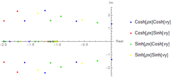
Set and the parameters in (80) and (81) as and , respectively. The bifurcation parameter in this example is . When , this type of connectivity models a population with inhibitory neurons. There is a Hopf bifurcation at with eigenvalues , see Figure 2, and corresponding eigenvector
In [16], a procedure is derived using the sun-star calculus to compute the Lyapunov coefficient for a Hopf bifurcation. For this we need the higher order Fréchet derivatives of (see [16]):
for and . Due to our choice of , and therefore, vanishes. This reduces the computation of the Lyapunov coefficient to the following equality
| (82) |
where is a closed contour containing and no other eigenvalues. The first Lyapunov coefficient is given by (see [8])
We use (82) as an identity for . To compute the contour integral in (82) we take for a small circle of radius around , for and perform a change of variables to obtain
We then compute the integral numerically by using an equidistant grid on of points, where we use that is periodic in .
To compute the resolvent we approximate (74) by truncating the infinite sum. For each grid point of above, we compute basis functions and basis functions . So we end up with basis functions . We use the Gramm-Schmidt procedure to get an orthonormal set with respect to the inner product. This enables us to find the coefficients by standard orthogonal projection. We find that using gives a good enough approximation for the purposes of this calculation, especially away from the boundary.
Finally, we need to compute the scalar and find that
| (83) |
This right hand side is, however, still a function of instead of a scalar, so naturally, this should be a constant function. We can use this fact to check our calculations. Using the values for the Hopf bifurcation above and , we see in Figure 3 that this is indeed the case. This results in a Lyapunov coefficient of . The negative sign of indicates a supercritical Hopf bifurcation.

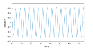
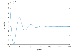
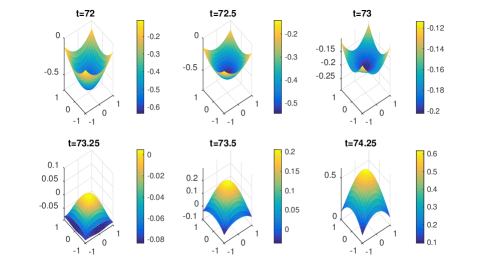
Some numerical time simulations were performed in Figure 4 and Figure 5 to illustrate the dynamic behavior of the solution of the neural filed model for parameter values before and beyond Hopf bifurcation.
6 Conclusions
We studied a neural field model with transmission delays and a connectivity kernel that is a linear combination of exponentials. Motivated by applications in neuroscience, we used a planar spatial domain, in particular a rectangle. This however, made the analysis more challenging.
We investigated in detail a model with a connectivity kernel that is a single exponential. To study the dynamics of the linearized equation, we completely characterised the spectrum. We constructed eigenvectors as solutions of the characteristic integral equation. We employed the fact that the integral equation is equivalent to a partial differential equation with a Robin-type boundary condition. This PDE can be separated into two differential equations of Sturm-Liouville type. We constructed a basis of solutions to these differential equations that is complete in . These basis functions allowed us to determine whether is part of the spectrum.
It is quite rare that one can completely characterise the spectrum of an operator acting on multivariate functions, such as partial differential or integral operators. It is sometimes possible to find some eigenvalues, but here we proved that we found them all. We investigated a numerical example of a population of inhibitory neurons. Using the developed theory, we detected a supercritical Hopf bifurcation.
The classical example of an excitatory and inhibitory population of neurons can be modeled using a connectivity kernel of two exponentials. In the special case when the rectangle is a square, we found eigenvalues and eigenfunctions, but we cannot conjecture that there are no more.
Acknowledgments
M. Polner was supported by the János Bolyai Research Scholarship of the Hungarian Academy of Sciences, the Hungarian Scientific Research Fund, Grant No. K129322 and SNN125119. Her research was also supported by grant TUDFO/47138-1/2019-ITM of the Ministry for Innovation and Technology, Hungary.
M. Polner would like to thank Prof. László Stachó for their valuable discussions on Section 4.2.
References
- [1] S.-i. Amari. Dynamics of pattern formation in lateral-inhibition type neural fields. Biological Cybernetics, 27(2):77–87, June 1977.
- [2] S. Coombes. Large-scale neural dynamics: Simple and complex. NeuroImage, 52(3):731–739, Sept. 2010.
- [3] S. Coombes, P. beim Graben, and R. Potthast. Tutorial on neural field theory. Springer, 2014.
- [4] Coombes Stephen and Laing Carlo. Delays in activity-based neural networks. Philosophical Transactions of the Royal Society A: Mathematical, Physical and Engineering Sciences, 367(1891):1117–1129, Mar. 2009.
- [5] K. Dijkstra, S. A. van Gils, S. G. Janssens, I. A. Kouznetsov, and S. Visser. Pitchfork-Hopf bifurcations in 1D neural field models with transmission delays. Physica D, 297:88–101, 2015.
- [6] K.-J. Engel and R. Nagel. One-Parameter Semigroups for Linear Evolution Equations, volume 63. Springer, 1999.
- [7] G. Faye and O. Faugeras. Some theoretical and numerical results for delayed neural field equations. Physica D, 239(9):561–578, 2010.
- [8] Y. A. Kuznetsov. Elements of Applied Bifurcation Theory. Springer Science & Business Media, Mar. 2013. Google-Books-ID: ZFntBwAAQBAJ.
- [9] P. M. Lima and E. Buckwar. Numerical solution of the neural field equation in the two-dimensional case. SIAM J. Sci. Comput., 37(6):B962–B979, 2015.
- [10] V. A. Marchenko. Sturm-Liouville Operators and Applications. Birkhauser Verlag, CHE, 1986.
- [11] P. L. Nunez. The brain wave equation: a model for the EEG. Mathematical Biosciences, 21(3):279–297, Dec. 1974.
- [12] M. Polner, J. J. van der Vegt, and S. A. van Gils. A space-time finite element method for neural field equations with transmission delays. SIAM Journal on Scientific Computing, 39(5), 2017.
- [13] R. M. Redheffer. Completeness of sets of complex exponentials. Advances in Mathematics, 24(1):1–62, 1977.
- [14] R. M. Redheffer and R. M. Young. Completeness and basis properties of complex exponentials. Trans. Amer. Math. Soc., 277:93–111, 1983.
- [15] L. Spek, Y. A. Kuznetsov, and S. A. van Gils. Neural field models with transmission delays and diffusion, 2019.
- [16] S. A. van Gils, S. G. Janssens, Y. A. Kuznetsov, and S. Visser. On local bifurcations in neural field models with transmission delays. J. of Math. Biol., 66(4-5):837–887, 2013.
- [17] R. Veltz and O. Faugeras. Stability of the stationary solutions of neural field equations with propagation delays. Journal of Mathematical Neuroscience, 1, 2011.
- [18] N. A. Venkov, S. Coombes, and P. C. Matthews. Dynamic instabilities in scalar neural field equations with space-dependent delays. Physica D: Nonlinear Phenomena, 232(1):1–15, Aug. 2007.
- [19] R. Vermiglio. Numerical approximation of the non-essential spectrum of abstract delay differential equations. Mathematics and Computers in Simulation, 125:56 – 69, 2016.
- [20] S. Visser, R. Nicks, O. Faugeras, and S. Coombes. Standing and travelling waves in a spherical brain model: The Nunez model revisited. Physica D: Nonlinear Phenomena, 349:27–45, June 2017.
- [21] H. R. Wilson and J. D. Cowan. Excitatory and Inhibitory Interactions in Localized Populations of Model Neurons. Biophysical Journal, 12(1):1–24, Jan. 1972.
- [22] H. R. Wilson and J. D. Cowan. A mathematical theory of the functional dynamics of cortical and thalamic nervous tissue. Kybernetik, 13(2):55–80, Sept. 1973.
- [23] R. M. Young. An introduction to nonharmonic Fourier series. Academic Press, 2001.
- [24] A. Zettl. Sturm-Liouville Theory. Mathematical Surveys and Monographs, vol. 121. American Mathematical Soc., Providence, RI, 2005.